Article

Modelling and Mitigating Wind Turbine Clutter in Space–Air Bistatic Radar

1
School of Electronics and Information, Northwestern Polytechnical University, Xi’an 710072, China
2
The Department 3, Wuhan Radar Academy, Wuhan 430014, China
*
Author to whom correspondence should be addressed.
Remote Sens. 2024, 16(14), 2674; https://doi.org/10.3390/rs16142674 (registering DOI)
Submission received: 20 June 2024 / Revised: 18 July 2024 / Accepted: 19 July 2024 / Published: 22 July 2024

Abstract

:
The extensive deployment of wind farms has significantly impacted the detection capabilities of space–air bistatic radar (SABR) systems. Although space–time adaptive processing techniques are available, their performance is significantly degraded, and even unable to suppress clutter. This paper explores the geometric configuration of the SABR system and the selection of detection areas, establishing a space–time clutter model that addresses the effects of wind turbine clutter (WTC). Expressions for spatial and Doppler frequencies have been derived to deeply analyze the characteristics of clutter spreading. Building on this, the paper extends two-dimensional space–time data to three-dimensional azimuth–elevation–Doppler data. It proposes a three-dimensional space–time multi-beam (STMB) strategy incorporating the Ordering Points to Identify the Clustering Structure (OPTICS) clustering algorithm to suppress WTC effectively. This algorithm selects WTC samples and applies OPTICS clustering to the clutter-suppressed data to achieve this effect. Simulation experiments further verify the effectiveness of the algorithm.

1. Introduction

The space-based early warning radar platform is gaining attention due to its high height, allowing for comprehensive coverage and a long warning time. However, the long-distance transmission loss of the radar system and the severe ground/sea clutter background pose significant challenges in terms of technical implementation and cost for target detection tasks [1,2,3,4,5]. The space–air bistatic radar (SABR) system uses satellites as the transmitters and aircraft as the receivers, which effectively alleviates the problem of long-distance signal transmission; at the same time, because the bistatic configuration can observe targets from different angles, there is the potential for anti-jamming and anti-stealth capabilities [6]. Furthermore, SABR is a more cost-effective solution than a spaceborne bistatic radar while providing broader coverage than an airborne bistatic radar [7,8]. Nevertheless, despite these advantages, SABR presents a more severe issue of clutter spectrum broadening than airborne bistatic radar (ABR). Additionally, with the large-scale construction of wind farms, the interference of multiple types of isolated point clutter, such as wind turbine clutter (WTC) on radar receivers, has become increasingly prominent. Taking wind turbine clutter as an example, the Doppler frequency shift interference signal of wind turbine clutter is constantly changing because of the rotation of the wind turbine blades, which leads to the occlusion of the target near the wind farm clutter unit and the increase in the false alarm rate caused by the clutter unit. Traditional methods have yet to be able to tackle this issue effectively [9].
After conducting thorough research, it was found that existing studies on SABR radar systems mainly concentrate on system design and demonstration [3,8,10,11,12,13], ground/air moving target detection [14,15,16], and SAR imaging [11,12,13,17,18,19,20]. Among these, the literature [10] mainly focuses on calculating the signal-to-noise ratio of satellite–airship bistatic radar. However, the literature mentioned above often overlooks the severe ground/sea clutter issue that SABR encounters when operating in the downward-looking mode; this problem is always present [21,22,23,24,25,26]. In the literature [22], a dimension-reduced STAP algorithm based on space–time two-dimensional sliding window processing is proposed for severely broadened main-lobe clutter. In reference [25], a sea clutter suppression method based on joint space–time–frequency adaptive filtering is proposed according to the time coherence analysis of sea clutter combined with a sub-aperture time-domain sliding window and improved subspace projection technology. Reference [26] proposed a range ambiguity clutter suppression algorithm considering the internal motion characteristics of sea clutter, AAPC, which solved the problem of the target detection blind area. Moreover, the transmitter–receiver separation geometry influences the clutter’s distance dependence [27,28,29,30,31], non-side-looking reception, extensive coverage, and the Earth’s rotation, resulting in slow-moving targets obscured in areas of severely broadened clutter. Even more severe is the large-scale construction of wind farms, which makes radar systems using airborne receiving platforms face severe WTC interference. This interference mainly includes direct interference caused by the high reflectivity of turbine components and Doppler interference caused by the movement of turbine blades. Groups of wind turbines also often cause diffraction of radar electromagnetic fields, creating shadow areas where monitoring is less efficient or blind spots in radar system detection.
Space–time adaptive processing (STAP) technology fully uses the multi-channel spatial information provided by the multi-channel radar and the time domain information provided by the coherent pulse train and realizes the effective suppression of clutter through the spatial and temporal two-dimensional adaptive filtering method. The key is to use adjacent training samples to estimate the covariance matrix accurately [32,33,34,35]. According to the RMB [36], to ensure that the performance loss of STAP is less than 3 dB, there should be at least twice as many independent and identically distributed (IID) training samples as the system’s degrees of freedom. However, problems such as transceiver separation, non-frontal side-looking reception [37], the Earth’s rotation [38,39,40], and interference from wind turbine clutter make it difficult for IID training samples to meet the requirements.
Wind turbine blades produce Doppler frequencies that continuously vary in the frequency domain, causing spectral broadening and wind turbine clutter to be distributed over multiple non-zero-frequency Doppler filter banks [41]. This affects the effectiveness of traditional displays and moving target detection. At the same time, it is difficult for traditional STAP to obtain enough independent and identically distributed training samples to estimate the covariance matrix in this case, so it cannot effectively suppress clutter. Various wind turbine clutter (WTC) suppression methods have been proposed in the literature [42,43,44,45,46,47,48,49]. Considering that a wind turbine blade echo is a non-stationary signal, Zhang et al. performed a time–frequency transformation on the echo signal. Then, they performed micro-Doppler suppression in the time–frequency domain according to the frequency difference of the rotating blades [42]. He et al. established a clutter map based on the wind turbine’s position. They used Doppler spread characteristics and the singular value decomposition method to suppress the WTC in the cluttered area to reduce the false alarm rate [43]. In addition, the method of reconstructing the wind turbine clutter first and then canceling the clutter from the echo signal has also been studied [41,44,45]. Karabayir et al. proposed the CLEAN method, which uses clutter features to reconstruct the wind turbine echo and uses it to eliminate clutter in the radar echo [44]; Wu et al. used spectrum estimation and compensation methods to eliminate the distance unit where WTC is located [45]. However, this method is only effective when the target and WTC are located in different distance units. In reference [41], the method of reconstructing echo data and then suppressing it is adopted for the case where clutter and target are in the same distance unit. Because a wind turbine echo has sparse characteristics, sparse signal processing can improve the clutter suppression performance [46,47,48]. Uysal and his team proposed a suppression method based on morphological component analysis, which involves reconstructing and converting wind turbines and target signals on different atomic bases to achieve WTC suppression based on the sparsity difference between each component [46]. Compared with reference [48], reference [47] has a large amount of computation, high dictionary redundancy, and relatively low reconstruction accuracy. In addition, Pan et al. proposed a method of extended Doppler clutter suppression using the modified reference signal in matched filtering processing [49]. The above studies suppress the wind turbine clutter from different stages of radar signal processing and transform domains, but most of these studies are based on ground active radar. There are few studies on the clutter suppression of radar wind turbines under the SABR configuration.
As mentioned above, when SABR works in the downward-looking mode, it not only faces distance-dependent space–time coupling to ground/sea clutter but also, the radar system with an airborne receiving platform as the receiving end will face serious WTC interference problems, which are more severe than those faced by ground-based radar. This results in a reduction in target detection performance. In this case, we propose a clutter suppression method based on the 3D space-time multiple-beam (3D-STMB) method combined with Ordering Points to Identify the Clustering Structure (OPTICS) clustering based on the clutter characteristics of large baseline bistatic radar affected by WTC. The main contributions of our work are as follows:
  • The study developed an accurate space–time clutter model for the SABR configuration. The model considered the impact of several factors, including the launch satellite orbit inclination, Earth’s curved surface, and Earth’s rotation. The study derived the bistatic equal distance, rings’ spatial frequencies, and Doppler frequency expressions;
  • Based on the above work, we explore the influence of wind turbines on radar clutter suppression. We established a clutter geometric model and a corresponding space–time echo model considering the influence of wind turbines under the SABR configuration. A three-dimensional STMB strategy incorporating the OPTICS clustering algorithm is introduced. This algorithm comprises two main phases: Initially, the 3D-STMB method is utilized for the initial clutter reduction. Subsequently, we leverage the distinct distribution characteristics of targets versus WTC using OPTICS clustering. This approach not only differentiates targets from clutter but also facilitates enhanced secondary clutter suppression, thereby improving the performance of the SABR system in a downward-looking configuration.
The remainder of this article is as follows. Section 2 describes the geometric configuration and space–time clutter model of SABR. Section 3 deduces the expression of the moving clutter received slant range under the influence of WTC, establishes the space–time clutter model of WTC, and analyzes the WTC. A clustering method based on 3D-STMB combined with OPTICS clustering for clutter characteristics is proposed. The simulation results are given in Section 4, and the research conclusions are shown in Section 5.

2. Geometric Configuration and Space–Time Clutter Model for SABR

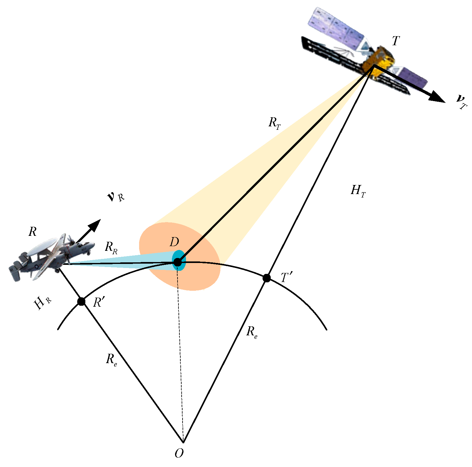
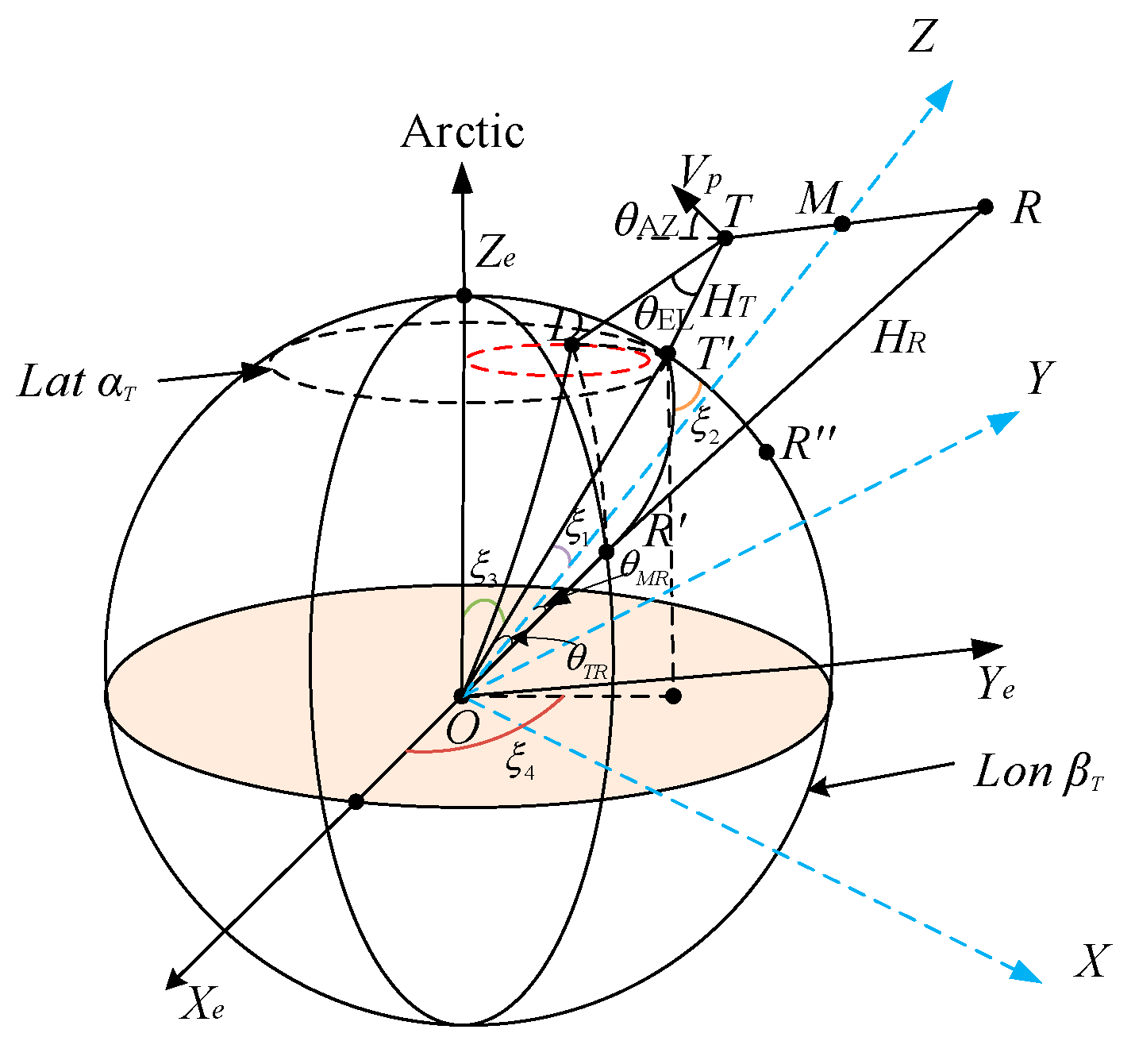
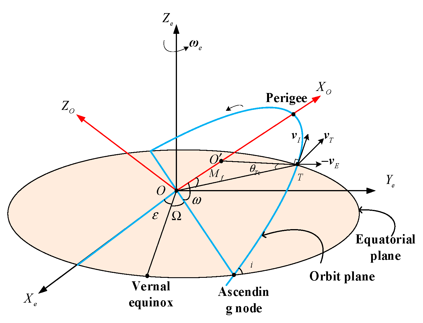
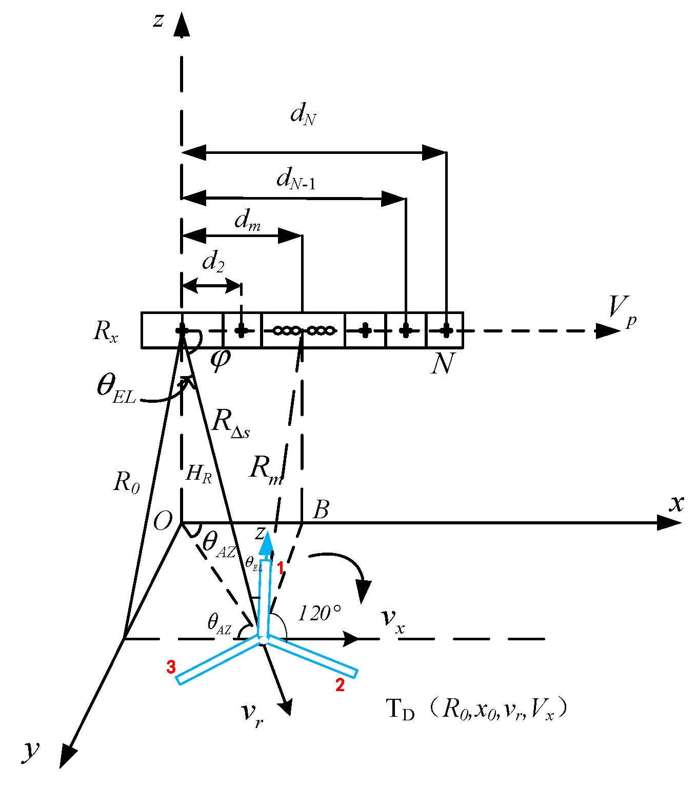
2.1. Geometric Configuration of SABR

The SABR system features a geometric structure diagram, represented in its typical form by Figure 1. The system consists of two main components: a transmitter (T) installed on a satellite and a receiver (R) installed on an airborne tethered platform. T′ and R′ denote the subsatellite points of the transmitter and receiver, respectively. Additionally, HT and HR represent the corresponding heights of the transmitter and receiver. At the same time, vT and vR indicate the velocity vectors of the transmitter and receiver, separately. D is any point on the clutter block, the slope distance to the transmitting end is RT, and the slope distance to the receiving end is RR, O is the center of the Earth, and Re is the radius of the Earth. For convenience, this article assumes that the Earth is a sphere.
R T max = ( R e + H T ) 2 R e 2   , R R max = ( R e + H R ) 2 R e 2  
Effective radar returns can only be produced if the transmitter and receiver in a radar system illuminate the same area despite the fact that they may cover different regions of the Earth’s surface. With the SABR system, the transmitting end is positioned at a high point, allowing it to cover a much larger area than the receiving end. Therefore, the effective clutter area primarily depends on the beam coverage of the receiver.
It is well known that clutter blocks on the isometric ring reach the receiver at the same time. In the SABR system, it is necessary to calculate the isometric and ring of the Earth’s surface. Figure 2 shows the clutter isometry and ring of SABR in the auxiliary coordinate system O-XYZ and M-XYZ′. Here, O represents the center of the Earth. Suppose M is the point in the center of the line connecting the transmitter T and the receiver R. The coordinate system uses the line connecting OM as the Z-axis and the straight line passing through the projection points of points T and R on the XOY plane and perpendicular to the Z-axis passing through the origin O as the X-axis [28]. The right-hand rule determines the coordinate system, with the Y-axis perpendicular to the X- and Z-axes.
In the auxiliary coordinate system O-XYZ, the transmitter T and receiver R coordinates are T = [Tx, 0, Tz] and R = [Rx, 0, Rz], respectively. Any point (x, y, z) on the center elliptical ring of the bistatic radar is located with T and R as the foci. On the ellipsoid surface, the general equations of each point on the ellipsoid surface conform to the following:
( x cos φ + ( z - m ) sin φ ) 2 a 2 + y 2 + ( - x sin φ + ( z - m ) cos φ ) b 2 = 1
In Formula (2), φ = arctan((RzTz)/(RxTx)) represents the elevation angle of the receiver relative to the transmitter, and m = (Rz + Tz)/2 represents the coordinates of the midpoint of the transceiver in the O-XYZ auxiliary coordinate system. The semi-major axis a of the ellipsoid is half the sum of the slant distances from the transmitter to the target point and from the target point to the receiver. When the two-way slant distance of the required receiving clutter equidistant ring is Rs, the semi-major axis of the ellipsoid is a = Rs/2. In addition, according to the geometric relationship, the minor semi-axis of the ellipsoid can be calculated as b = a 2 ( R x T x 2 + R z T z 2 ) / 4 .
The transmitter’s coordinates in the geocentric fixed coordinate system can be determined by six orbit elements and the orbit time. The receiver’s coordinates can be determined by longitude, latitude, and height. Therefore, we can express the coordinates of the transmitter and receiver as x T E C F , y T E C F , z T E C F and x R E C F , y R E C F , z R E C F , respectively. Additionally, the longitude and latitude of the subsatellite points T′ and R′ can be expressed as (αT, βT) and (αR, βR), separately. Using this information, we can express the coordinates of the center M in the ECF coordinate system.
( x M E C F , y M E C F , z M E C F ) = ( ( x T E C F + x R E C F ) 2 , ( y T E C F + y R E C F ) 2 , ( z T E C F + z R E C F ) 2 )
According to the geometric relationship, it can be known that the angle θTR between vector O T and vector O R and the angle θMR between vector O M and vector O R in Figure 2 are expressed as
θ T R = arccos ( O T O R | O T | | O R | )   , θ M R = arccos ( O M O R | O M | | O R | )
The angle between vector O M and vector O T is θMT = θTRθMR. Therefore, the transmitter and receiver coordinates in the O-XYZ auxiliary coordinate system are, respectively,
( x T , y T , z T ) = [ ( R e + H T ) sin θ M T 0 ( R e + H T ) cos θ M T ]
( x T , y T , z T ) = [ ( R e + H R ) sin θ M R 0 ( R e + H R ) cos θ M R ]
Next, we need to translate the origin of the auxiliary coordinate system O-XYZ along the positive direction of the Z-axis to the midpoint M of TR. We will use point M as the new coordinate origin and rotate the M-XYZ coordinate system around the positive direction of the Y-axis by angle φ. This will allow us to obtain a new coordinate system, M-XYZ′, as shown in Figure 2. Points T and R are located on the X-axis of the new coordinate system, and the points on the ellipsoid can be expressed as parametric equations:
{ x = a cos ρ y = b sin ρ sin γ z = b sin ρ cos γ
Here, ρ represents the angle between the line MD connecting the origin M of the new coordinate system and point D on the ellipsoid surface and the positive direction of the X′ axis, ranging from 0 to 2π, and γ represents the angle between the MD and the positive half-axis direction of the Z′ axis. From the parametric Equation (7) of the simultaneous ellipsoid coordinate system in M-XYZ′ and the general Equation (2) of the auxiliary coordinate system O-XYZ, we can obtain the position of each point on the ellipsoid surface in the auxiliary coordinate system O-XYZ. The parametric equation can be expressed as
{ x = a cos ρ cos φ b sin ρ cos γ sin φ y = b sin ρ sin γ z = m + a cos ρ sin φ + b sin ρ cos γ cos cos γ
Each point on the equidistant elliptical ring on the Earth’s surface satisfies the ellipsoid equation and the Earth’s spherical equation with O as the center.
x 2 + y 2 + z 2 = 1
Simultaneous Equations (7) and (8) show that the parameter angles of each point on the clutter isometry ring satisfy
cos γ = R e ( a 2 cos 2 ρ + b 2 sin 2 ρ + m 2 + 2 m a cos ρ sin φ ) 2 m b sin ρ cos φ
Therefore, when the ρ value satisfies Equation (10) in the range of 0 to 2π, and the calculated γ belongs to the points in the range of 0 to π to form a bistatic early warning radar receiving clutter isometry ring, Equation (8) can be solved by substituting the calculated parameter angles ρ and γ of the ellipsoid equation into it. The precise coordinates of the receiving clutter equidistant elliptical ring in the O-XYZ auxiliary coordinate system can be obtained.
The Earth-centered Earth-fixed coordinate system, O-XeYeZe, is commonly used as the unified coordinate system. The transformation from the auxiliary coordinate system, O-XYZ, to O-XeYeZe can be done by using the process shown in Figure 3. Firstly, the YOZ plane is rotated clockwise by ξ 1 degrees around the OY axis to make the OZ axis coincide with OT. Then, counterclockwise rotation by ξ 2 degrees is completed around the OZ (OT) axis. This brings points T′ and R″ into the same meridian coil. After that, ξ 3 degrees clockwise rotation is finished around OY so that the OZ axis coincides with OZe. Lastly, the OZe R″ plane is rotated clockwise around OZe by ξ 4 degrees to the OXeZe plane. Therefore, the coordinate system’s transformation from O-XYZ to O-XeYeZe includes four sub-steps, which can be written as
u e = [ x e y e z e ] = [ cos ( ξ 4 ) sin ( ξ 4 ) 0 sin ( ξ 4 ) cos ( ξ 4 ) 0 0 0 1 ] [ cos ( ξ 3 ) 0 sin ( ξ 3 ) 0 1 0 sin ( ξ 3 ) 0 cos ( ξ 3 ) ] [ cos ( ξ 2 ) sin ( ξ 2 ) 0 sin ( ξ 2 ) cos ( ξ 2 ) 0 0 0 1 ] [ cos ( ξ 1 ) 0 sin ( ξ 1 ) 0 1 0 sin ( ξ 1 ) 0 cos ( ξ 1 ) ] [ x y z ]
Among them, ξ 2 = a r c c o s c o s α R c o s α R κ c o s β R β T + s i n α R s i n α T κ c o s 2 κ / 1 c o s 2 κ   κ = a r c c o s c o s α T c o s α R c o s β R β T + s i n α T s i n α R , ξ 1 = θ T R θ M R , ξ 3 = π / 2 α T , ξ 4 = β T .

2.2. Doppler Frequency and Spatial Frequency

Consider a scenario where a satellite orbits the Earth in an elliptical path, as illustrated in Figure 4. In this context, Mf, Ω, and ω denote the actual periapsis angle, ascending node right ascension, and perigee argument, respectively. The orbital inclination is denoted by i, and ε represents the angle between the equinox and the zero longitude. The derivation considers the curvature of the Earth and its rotation by utilizing a vector form of velocity to calculate the Doppler frequency of the clutter. A space-based launch platform comprises two Doppler frequency components. One component is produced by the platform’s motion, and the other is caused by the Earth’s rotation. For convenience, we can consider the Earth stationary and transmit its rotation to the satellite [50]. Hence, the resultant velocity vector induced by the Earth’s rotation on the satellite can be denoted as v E e = ω e × ρ T e , wherein the angular velocity vector of rotation is represented by T, and ω e = [ 0   0   ω e ] T ; the Earth’s rotation angular velocity is denoted as ω e = 7.292749 × 10 5 rad/s. Additionally, ρ T e signifies the position vector of the transmitter T in the O-XeYeZe coordinate system.
The satellite’s inertial velocity vector is located on the orbital plane and can be expressed as
v I e = v I e ( u T O e × z O )
where v I e = G ( 2 / ( H r + R e 1 ) / a ) represents the size of the satellite’s inertial velocity, G denotes the Earth’s gravitational constant, a represents the semi-major axis of the ellipse, u T O e × z o is defined as the unit vector in the direction of the satellite’s inertial velocity, and u T O e is defined as the unit vector in the direction perpendicular to the satellite’s inertial velocity TO′ on the orbital plane. The angle θ R = a r c t a n e s i n M f / 1 + e c o s M f is between TO′ and TO [51], where e represents the orbital inclination angle. u T O e   can be expressed as a result.
u T O e = [ cos θ T c sin θ T c 0 sin θ T c cos θ T c 0 0 0 1 ] u T O e
Among them, u T O e = ( ρ T e ρ O e ) / | | ρ T e ρ O e | | is defined as the unit vector in the direction from the transmitter T to the center of the Earth, ρ O e represents the position vector of the Earth’s center O in the O-XeYeZe coordinate system, and zo is defined as the unit vector of the z0 axis. According to the conversion relationship between the O-XOYOZO and O-XeYeZe coordinate systems, the coordinates of zo under O-XOYOZO can be obtained as
z O = [ cos ω sin ω 0 sin ω cos ω 0 0 0 1 ] [ 1 0 0 0 cos i sin i 0 sin i cos i ] [ cos ( ε + Ω ) sin ( ε + Ω ) 0 sin ( ε + Ω ) cos ( ε + Ω ) 0 0 0 1 ] [ 0 0 1 ]
Then, the transmitted Doppler frequency of ground clutter unit D can be expressed as
f d T = v T e · u T D e λ = ( v I e v E e ) · u T D e λ
where λ is defined as the wavelength, u T D e = ( ρ T e ρ D e ) / | | ρ T e ρ D e | | represents the unit vector in the direction from the transmitter T to the ground clutter block D, and ρ D e   represents the clutter block D position vector in the O-XeYeZe coordinate system.
Assuming the receiving antenna array undergoes column subarray synthesis, it is evenly divided into N identical spatial subarrays along the azimuth dimension. In the O-XYZ coordinate system, the receiving antenna array is located on the O-XZ plane, the n-dimensional linear array is parallel to the X-axis, and the unit vector u = [1 0 0]T is along the array axis direction. Using Equation (11), we can obtain the unit vector ue along the array axis direction in the O-XeYeZe coordinate system. Consequently, the spatial frequency of the ground clutter block D can be expressed.
f s = d λ u e u R D e
where d is the array element spacing, u R D e = ( ρ R e ρ D e ) / | | ρ R e ρ D e | | represents the unit vector in the direction from the receiver R to the clutter block D, and ρ R e represents the position vector of the receiver R in the O-XeYeZe coordinate system. We assume that the platform’s velocity vector component is v R 0 in the O-XYZ coordinate system. During the flight, there is an oblique side angle α between the average direction of the receiving platform’s array antenna and the direction of movement. We first introduce the Rodrigues rotation formula to convert velocity vectors easily, which calculates three-dimensional space. For two vectors in three-dimensional space, k = k x k y k z T and v = v x v y v z T , k is the unit vector. v can rotate θrot around k to get vrot; a right-handed spiral determines the direction. Finally, we can express the above process through matrix operations [32].
v r o t = R rot ( k , θ r o t ) v
Among them, the rotation matrix is calculated using the following formula:
R rot ( k , θ r o t ) = E cos ( θ r o t ) + ( 1 cos ( θ r o t ) ) [ k x 2 k x k y k x k z k y k x k y 2 k y k z k z k x k z k y k z 2 ] + sin ( θ r o t ) [ 0 k z k y k z 0 k x k y k x 0 ]
E is the third-order unit matrix. Therefore, the velocity vector of the receiving platform after considering the bevel angle can be expressed as
v R = R r o t ( O R | O R | , α ) v R O
From Equation (11), we can get the actual velocity vector v R e of the receiver and the received Doppler frequency of the ground clutter block D in the O-XeYeZe coordinate system.
f d R = v R e · u R D e λ
Combining the transmit Doppler frequency in Equation (15) and the receive Doppler frequency in Equation (20), the Doppler frequency of ground clutter block D is finally obtained.
f d = f d T + f d R

2.3. Clutter Signal Model

Suppose there are N receiving channels, and K pulses are transmitted during the coherent processing interval. Under ideal conditions, the sampling data of the lth range ring clutter (ignoring the noise term) for the kth pulse of the nth channel (column subarray) can be expressed as follows:
c l ( n , k ) = i = 1 N c A i exp ( j ( n 1 ) ω s i + j ( k 1 ) ω t i )
Among them, n = 1, 2,…, N; k = 1, 2,…, K; l = 1, 2,… , L; Nc represent the equal distance and the number of clutter blocks in the ring; ωsi = 2πfsi, ωti = 2πfdi/fr, and Ai the normalized spatial frequency, normalized Doppler frequency, and echo signal amplitude of the ith clutter block, respectively.
The received echo signals are superimposed into an NK-dimensional space–time snapshot, and the clutter signal model of the lth isometry ring can be expressed as
c l = [ c l ( 1 , 1 ) , c l ( 1 , 2 ) , , c l ( 1 , K ) , c l ( 2 , 1 ) , , c l ( N , K ) ] T     = i = 1 N c A i s s ( f s i ) s t ( f d i ) = i = 1 N c A i s i
In the formula, si represents the space–time steering vector, ss(fsi) and st(fdi) are separately represented as the space steering vector and the time steering vector, and their form is
s s ( f s i ) = [ 1 exp ( j ω s i ) exp ( j ω s i ( N 1 ) ) ] T s t ( f s i ) = [ 1 exp ( j ω t i ) exp ( j ω t i ( K 1 ) ) ] T
The echo signal corresponding to the lth distance and ring can be expressed as
x l = c l + n l
At this point, the construction of the space–time clutter model and its echo signal of the SABR system has been completed.
As depicted in Figure 5, the red box represents the latitude and longitude of the sending platform, and the blue box represents the latitude and longitude of the receiving platform; the black solid line indicates the coverage of the receiver. Considering the distribution of iso-range rings, selecting the eastern side of the receiving platform for the detection area is advisable. This choice is based on the moderate variation in iso-range rings on this side and the small range of beam elevation angles between the transmitting and receiving platforms. Therefore, in scenarios characterized by ‘high platform transmitting, low platform receiving’, the eastern side is deemed suitable for detection. Furthermore, as shown in Figure 6a and Figure 6b, the configuration design with GEO and MEO as the transmitting platforms and the aerial platform as the receiving end are defined as Scenario 1 and Scenario 2, respectively. The parameters of the received platform are shown in Table 1.

3. Modelling and Suppression for WTC

3.1. Geometric Model and Space–Time Signal Model of WTC

3.1.1. Geometric Model

A schematic diagram of the observation geometry of the receiving platform is provided, as illustrated in Figure 7, using the array plane parallel to the velocity direction of the platform as an example. The x-axis is parallel to the direction of the phase center arrangement, the y-axis is perpendicular to the track direction, and the z-axis is perpendicular to the ground and upward. The speed Vp of the receiving platform is parallel to the x-axis (the speed of movement along the x-axis is specified as positive), which is equivalent to the number of array elements, N. The number of pulses is K, dm represents the distance between the mth array element and the transmitting channel (reference channel) along the track, HR is the height of the receiving platform, θAZ and θEL are the moving target TD (taking blade one as an example, assume that the fan blade is parallel to the z-axis at this time) relative to the azimuth angle and pitch angle of the array direction, φ represents the space cone angle between the moving target TD and the array direction, and cosφ = sinθELcosθAZ. Assume that when the azimuth slow time tm = 0, the moving target TD is at (R0, x0) (it is known that the height of the windmill is much smaller than the slant distance between the platform and the windmill), and the target moves along the radial and platform velocity directions in the slant distance plane. The speeds are vr and vx, respectively. Typically, R0   d m , R0vrTm, and R0VpTm, where Tm represents slow time accumulation, and Rm is the receiving slope distance of the mth equivalent channel.
R m ( t m ) = ( v r x t m + d m ) 2 + ( R 0 v r t m ) 2 R 0 v r t m + ( v r x t m + d m x 0 ) 2 2 R 0
Among them, vrx = Vpvx represents the relative speed of the moving target along the track direction. Within a coherent processing interval (CPI), (vrxtm)2/(2R0) can be ignored, and d m 2 / 2 R 0 , R0, and (dmvrx/R0)tm can be compensated, so Equation (26) can be simplified.
R m ( t m ) v r t m x 0 v r x R 0 t m x 0 d m R 0
From the above geometric relationship, we can get x 0 / R 0 = s i n θ E L c o s θ A Z = O T D / R 0 · x 0 / O T D = c o s φ , and because vrx = Vpvx, vr = vxcosφ + vzcosθEL, the above formula can be simplified to
R R ( t m ) v r t m ( V p v x ) t m cos φ d m cos φ
In the same way, it can be obtained that high orbit vrx = VpTvxVpT, where VpT is the radial velocity of the transmitting end along the receiving platform.
R T ( t m ) v r t m ( V p T v x ) t m cos φ d T cos φ

3.1.2. Space–Time Signal Model of Windmill Motion Clutter

In the high-transmit-and-low-receive mode, the signal delay corresponding to the mth receiving channel is
t d = R m ( t m ) + R T ( t m ) c = 2 v r t m ( V p T + V p 2 v x ) t m cos φ ( d m + d T ) cos φ c
When the transmitter is located at GEO, VpT >> Vp, VpT >> vx, Formula (30) is simplified to
t d = ( R m ( t m ) + R T ( t m ) ) / c = ( 2 v r t m ( V p T ) t m cos φ ( d m + d T ) cos φ ) / c
The above formula can be divided into a time part (−2vrtm − (VpT)tmcosφ) and a space part (−(dm + dT) cosφ)/c. Let dT = 0 and substitute it into the expression of the echo signal to obtain the spatial angular frequency and normalized Doppler frequency, respectively:
{ ω s = 2 π f s = d λ / 2 π sin θ E L cos θ A Z ω t = 2 π f d / f r
Among them, when the transmitter is in a geosynchronous orbit with an orbital inclination of zero, the Doppler frequency of the receiving platform is
f d = ( ( V p 2 v x ) cos φ + 2 v r ) / λ = ( ( V p 2 v x ) cos φ + 2 ( v x cos φ + v z cos θ E L ) ) / λ = ( V p cos φ + 2 v z cos θ E L ) / λ
Vp is the speed of the receiver platform, fr is the pulse repetition frequency, and vx and vz are the x-axis and z-axis components of the linear velocity of the windmill blades at different positions, separately. Its vector form can be expressed as
v x = v T D x ^ v z = v T D z ^
x ^ = [ 1   0   0 ] T and z ^ = [ 0   0   1 ] T are unit vectors. And v T D represents the linear velocity vector of each point on the fan blade:
v T D = ω T D × ( u β O T D m ) ,   m = 1 , 2 , , M n
ω T D = 00 ω T D T , where ω T D is the angular velocity of the windmill, u β = c o s β 0 s i n β 0 1 0 s i n β 0 c o s β is the rotation matrix of the vector O T D m in the left-hand coordinate system, β = 2 π n / 3 + θ 0 = 2 π n / 3 + ω T D t , n = 0,1 , 2 is the arc value of the fan blades 1-3 relative to the z-axis, and t is the time; O T D m is the fan blade center O. The vector representation to a point on the fan blade, Mn, is the total number of points selected on a single fan blade; θ0 is the angle between fan blade one and the z-axis at the initial moment.
It is easy to obtain the echo signal of the lth WTC by using Equations (23)–(25).
c W T C l = i = 1 N c A f c i s W T C = i = 1 N c A f c i b ( ω t i ) a ( ω s i )
Among them, b ( ω t i ) , a ( ω s i ) , and A f c i , respectively, represent the time Doppler frequency, spatial Doppler frequency, and clutter amplitude of the lth WTC.
Using the length of fan blade one as an example, the distance resolution unit (dR) is 60 m. Assume that when fan blade one rotates from the z-axis, fan blade three is pointed at the main beam; then the rotation time is t m d = θ 0 / ω T D = 120 π / 180 θ E L / ω T D .
As illustrated in Figure 8, the angle between the fan blades is 120°. The scattering points on the windmill blades are grouped such that those between blades one and two fall within the same range gate, while those between blades two and three occupy a different range gate. Given the blade length of the windmill and the radar’s resolution unit, it is apparent that the wind turbine clutter (WTC) motion clutter caused by the rotation of a single windmill is primarily distributed across two adjacent distance gates.
Take the typical megawatt wind turbine as an example. This type of fan starts at a wind speed of 3 m/s and generally rotates at 12–13 r/min at a wind speed of about 6–8 m/s. Therefore, the angular velocity of a windmill rotating at 12–13 r/min is ω T D = 1.36   r a d / s , assuming there are 25 strong scattering points on each fan blade and the distance between each scattering point is 3 m. Refer to Figure 8b. From the analysis of blade distribution, it is evident that the 50 strong scattering points on blades one and two, along with the 5 strong scattering points on blade three nearest to the blade center, are all within the 120th distance gate. The additional 20 scattering points on blade three are within the 119th range gate. Scenario 1 corresponds to the transmitter being in a geosynchronous orbit (GEO), while Scenario 2 has the transmitter in the middle orbit (MEO). The simulation results are illustrated in the figure below.
Comparing Figure 9a,d, it can be seen that although both scenarios involve side-looking reception, the main clutter area in Scenario 2 is far from the position where the Doppler center frequency is zero, compared with Scenario 1. This shift is primarily due to the more significant relative motion between the transmitter’s orbit and the ground clutter in Scenario 2. Analysis of Figure 9c,f reveals a complex interaction: wind turbine blades cause continuous shifts in Doppler frequency across the frequency domain, leading to a broadening of the spectrum. This results in wind turbine clutter spreading across multiple centers with non-zero center frequencies. Figure 9b,e illustrate another critical issue: if a target is located between range gate 120.5 and range gate 118.5, it risks being obscured by wind turbine clutter (WTC), resulting in potential target loss.
Therefore, developing effective methods to suppress WTC is crucial.

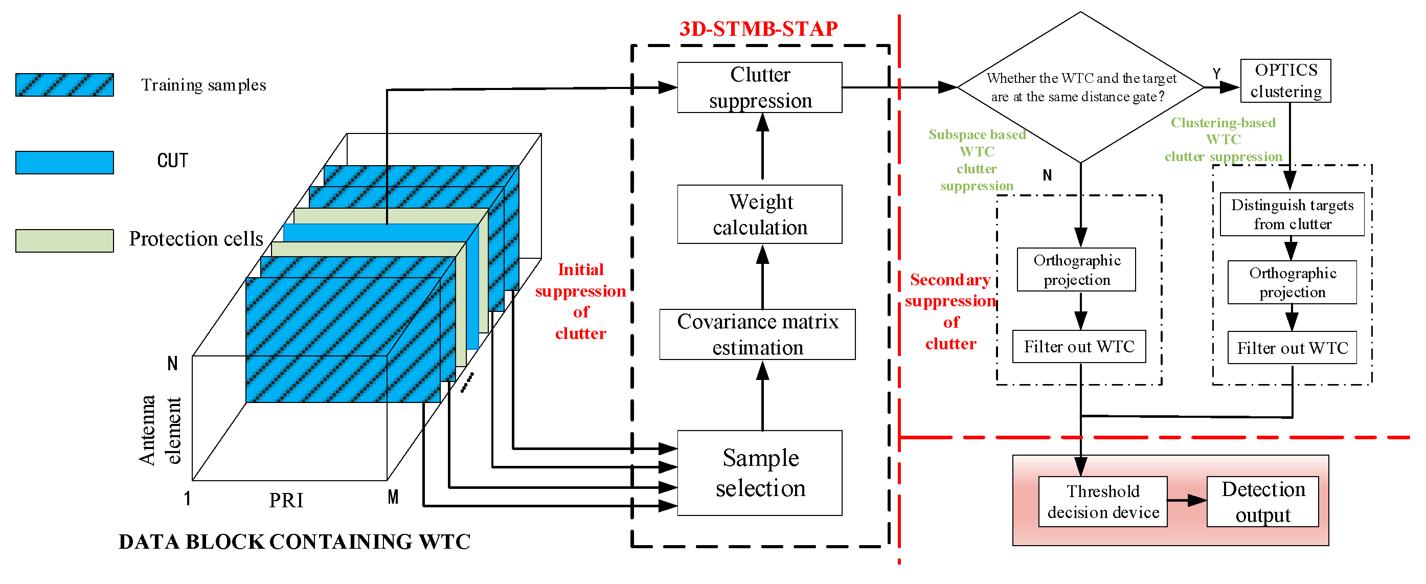
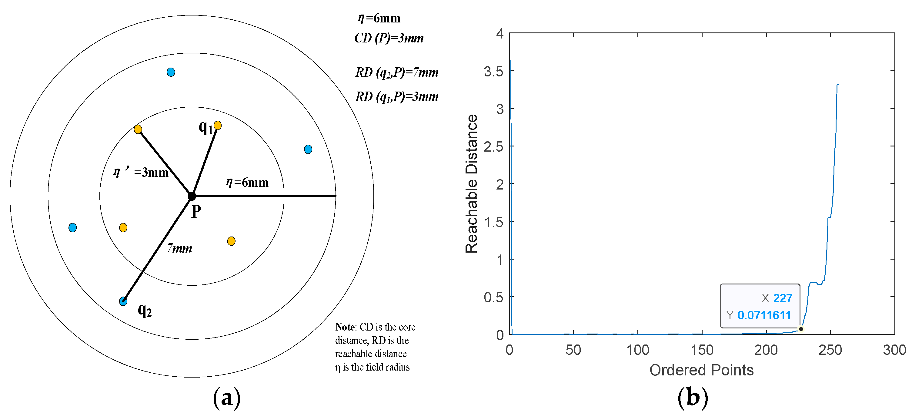
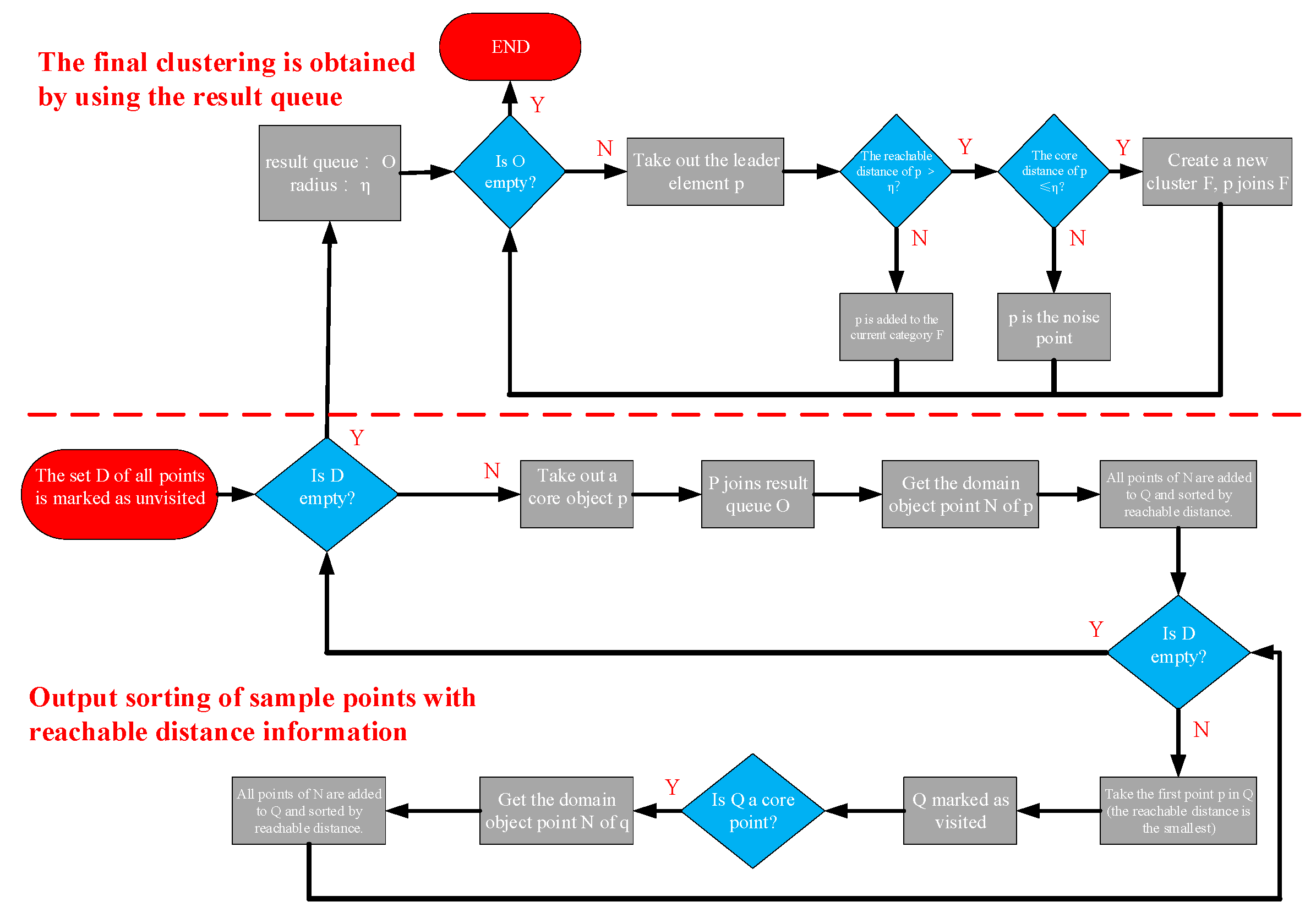
3.2. Clutter Suppression Based on STMB Combined with OPTICS Clustering
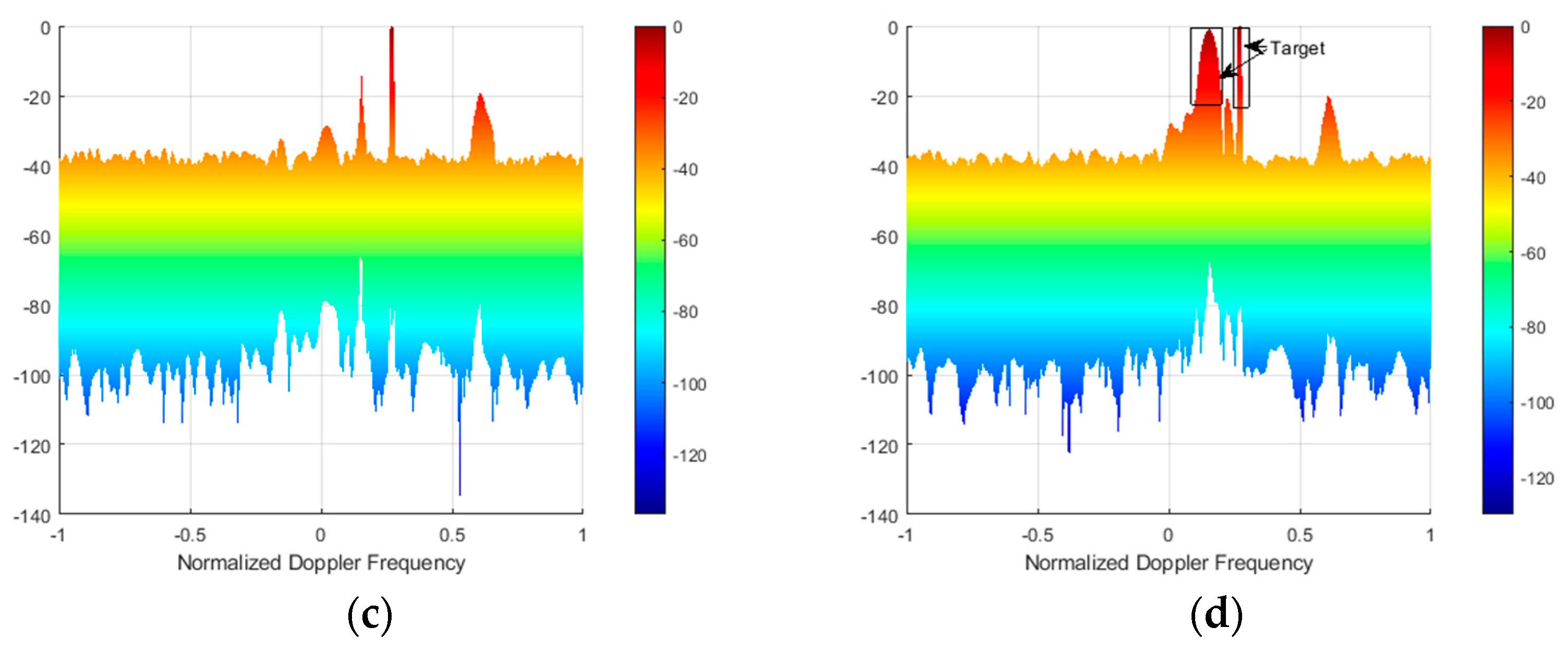
Aiming at the problem that the clutter diffusion of wind turbines is severe and the target is difficult to detect when it falls in the range gate where the wind turbine clutter is located, as well as its adjacent range gate, an STMB clutter suppression algorithm combined with the OPTICS clustering algorithm is proposed. First, the echo is subjected to STMB clutter suppression. If the target and the wind turbine are in different range gates, singular value decomposition (SVD) is used to identify the eigenvector associated with the maximum eigenvalue from the echo, thereby creating a clutter subspace. This subspace is then combined with the orthogonal subspace method to suppress WTC. Conversely, when the target and the wind turbine are in the same range gate, OPTICS clustering is performed on the processed echo data to separate the target from the clutter. Subsequently, SVD is used to filter out the clutter. Finally, threshold judgment and detection are performed on the processed echo data. The entire process is depicted in Figure 10.
The STMB algorithm reduces the demand for training samples while reducing the amount of calculation [52]. In this paper, 2D-STMB is extended to the 3D-STMB algorithm, which effectively suppresses the non-stationarity of bistatic radar clutter. The right side of the red dotted line represents the secondary suppression of wind turbine clutter (WTC) using the orthogonal subspace method combined with the OPTICS clustering algorithm. Here, the term ‘clutter’ refers to WTC that remains after initial space–time adaptive processing. Additionally, the STMB algorithm enhances clutter suppression by selecting WTC samples located at various distances from the target. This selection process helps to ensure that the energy of the ground clutter is lower than that of the target, which is conducive to using the OPTICS clustering algorithm to distinguish the target and suppress the WTC. Figure 11 and Figure 12 illustrate the 3D-STMB algorithm and the simulation results, respectively.
Figure 12 compares range–Doppler (RD) spectra for clutter suppression using the 3D-STMB algorithm on echo data containing wind turbine clutter (WTC) samples, before and after sieving. As demonstrated in Figure 12a,b, directly applying clutter suppression to datasets with WTC can effectively reduce WTC from wind turbines 2-3. However, this approach struggles to suppress ground clutter between these turbines, resulting in higher energy levels for WTC and ground clutter than the target. Thus, sieving the sample containing WTC is necessary before suppressing echo data.
The OPTICS algorithm was proposed by Ankerst M, Breunig M, and Kriegel H-P in 1999 [53]. It is a density-based spatial clustering algorithm. The following describes the OPTICS algorithm based on the echo data of the 119th and 120th range gates containing WTC after STMB suppression. Initially, echo data within the specified range gate is standardized. Subsequently, using the OPTICS algorithm, a reachability plot is constructed based on the minimum domain radius η (infinity) and a predetermined threshold for core points. Appropriate η values are then selected from the reachability plot for clutter clustering. Additionally, the concepts of core distance and minimum reachable distance are illustrated in Figure 13a, while the reachability plot is depicted in Figure 13b. OPTICS clustering algorithm flow chart, as shown in Figure 14.
Here, D is the set to be clustered, Q is the ordered queue, and O is the result queue.

4. Simulation

This section presents simulation experiments to verify the effectiveness of the clutter suppression algorithm proposed in Section 3. The method is based on 3D-STMB and OPTICS clustering, and a comparative analysis is conducted with the clutter suppression method that only uses the 3D-STMB algorithm. Table 2 gives the receiving platform and radar system parameters. Two hundred training samples are used, and the WTC is located at the 119th–120th range gate. Target 1 is located at the same isometry ring as the wind turbine (120th isometry ring), with a radial speed of v1 = 65 m/s. Target 2 is located at the 116th isometry ring, with a radial speed of v2 = 37 m/s. Receiver platform and radar system parameters, as shown in Table 2.

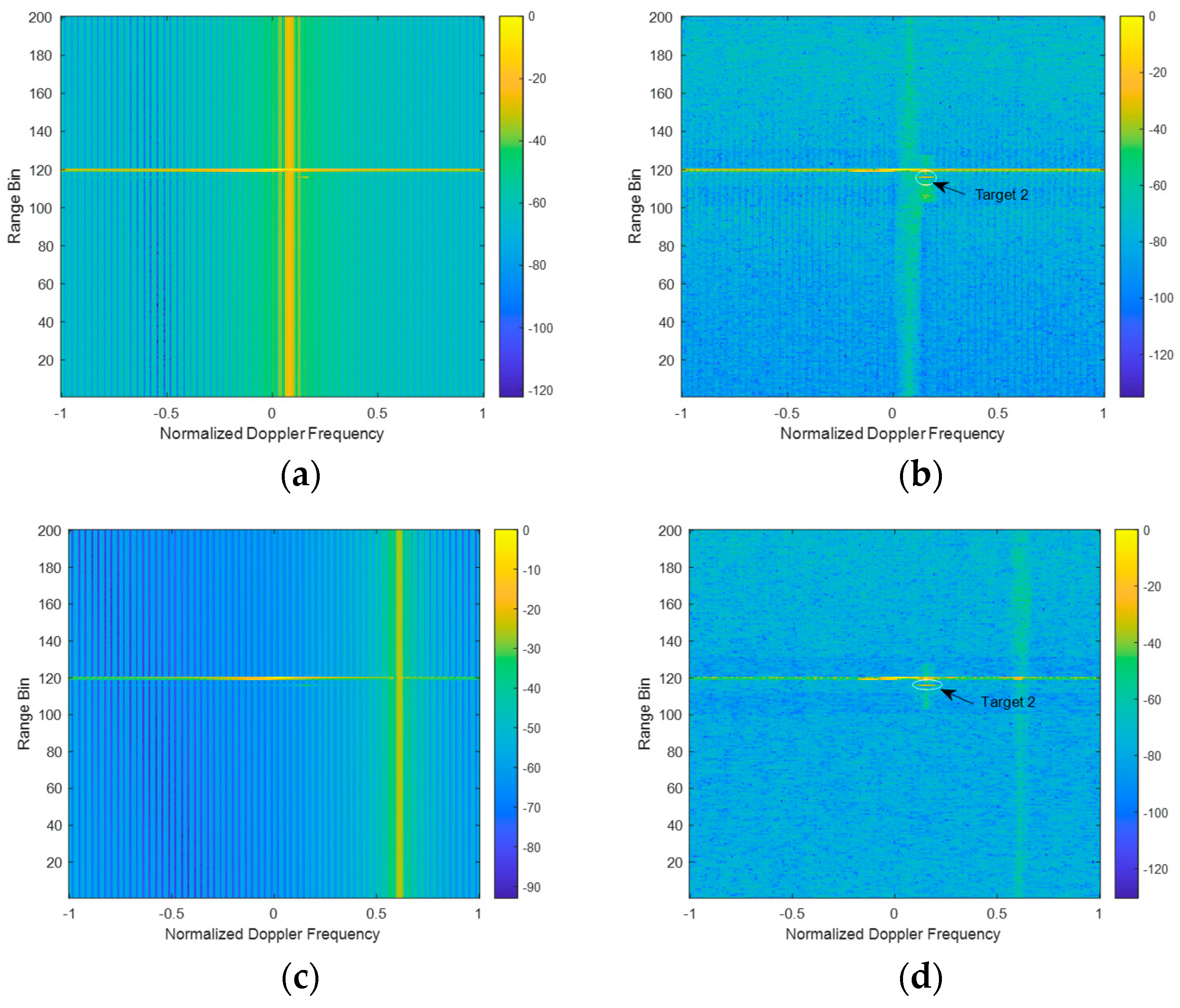
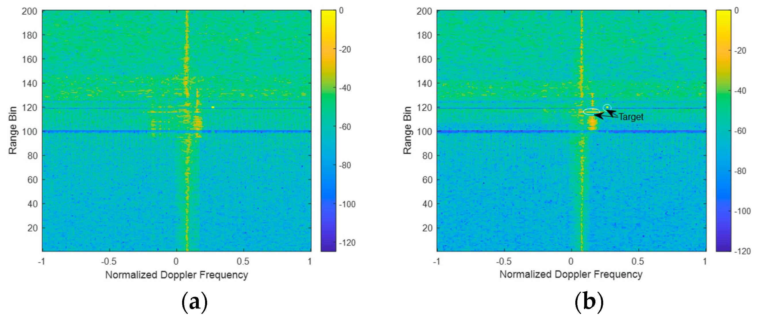
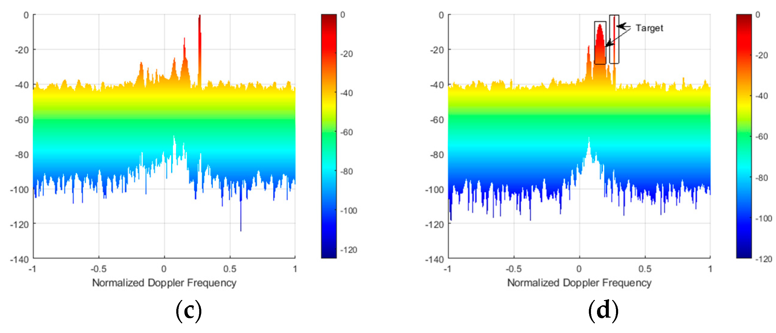
4.1. Single Wind Turbine

This section addresses the impact of a wind turbine on clutter suppression under typical wind speeds. As can be seen from Figure 15, the target and the wind turbine are in the same equidistant ring, and the WTC blocks the target. Despite the application of STMB for clutter suppression, target 1 remains obscured with the presence of WTC at the 119th–120th isometry rings, indicating the ineffectiveness of the STMB algorithm in suppressing WTC. The subsequent Figure 15 and Figure 16 show that the orthogonal subspace method can effectively suppress the WTC after the initial clutter suppression using STMB, and target 2 is seen. Finally, clutter suppression is conducted where target 1 coincides with WTC at the same range gate, whereas target 2 is located at a different range gate. As shown in Figure 17, target 1 and target 2 are visible in the RD spectrum after OPTICS clustering for clutter suppression. Target 1 is located at (fd1, 120), where fd1 = 2 (v1 + vRcosφ)/(λfr) = 0.27 Hz; target 2 is located at (fd2, 116), where fd2 = 2(v2 + vRcosφ)/(λfr) = 0.15 Hz is consistent with the theoretical value.

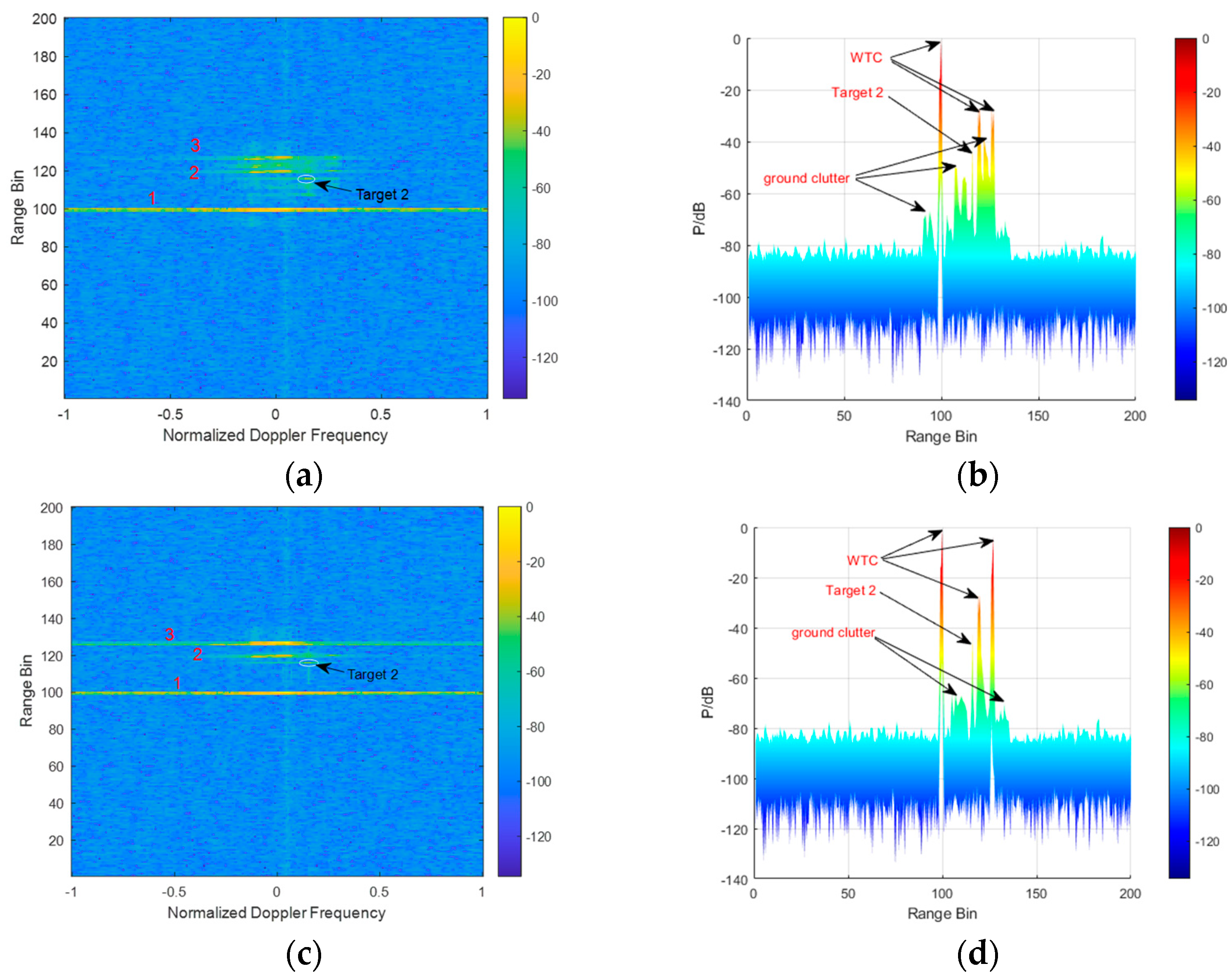
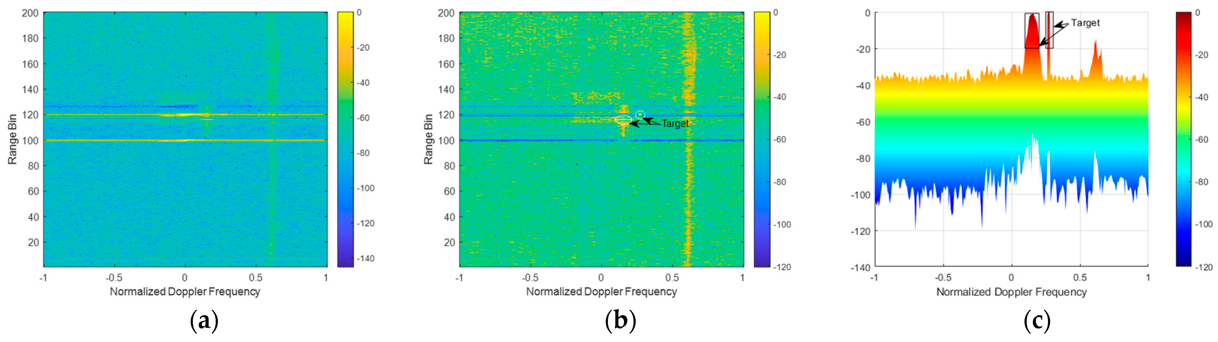
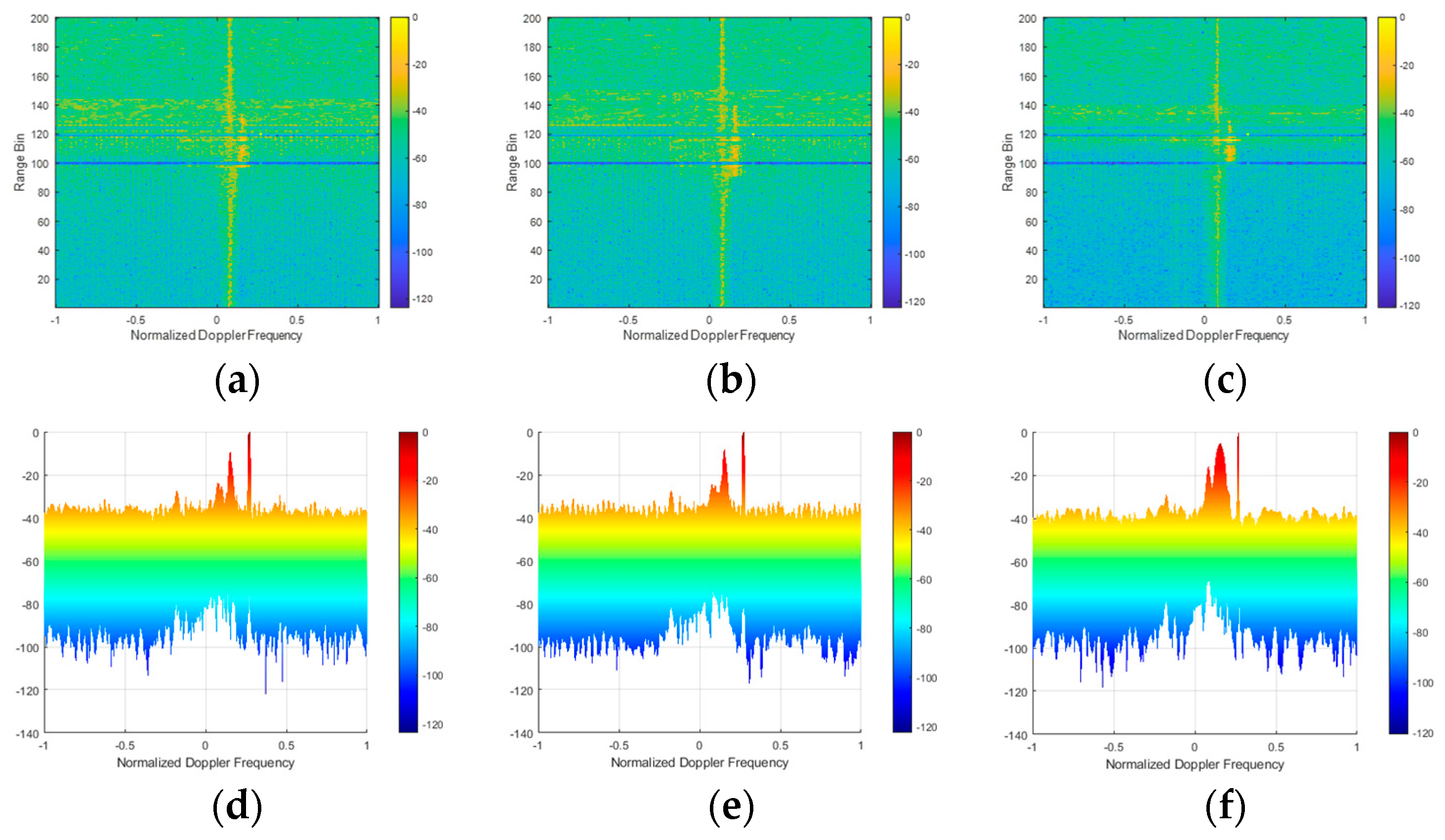
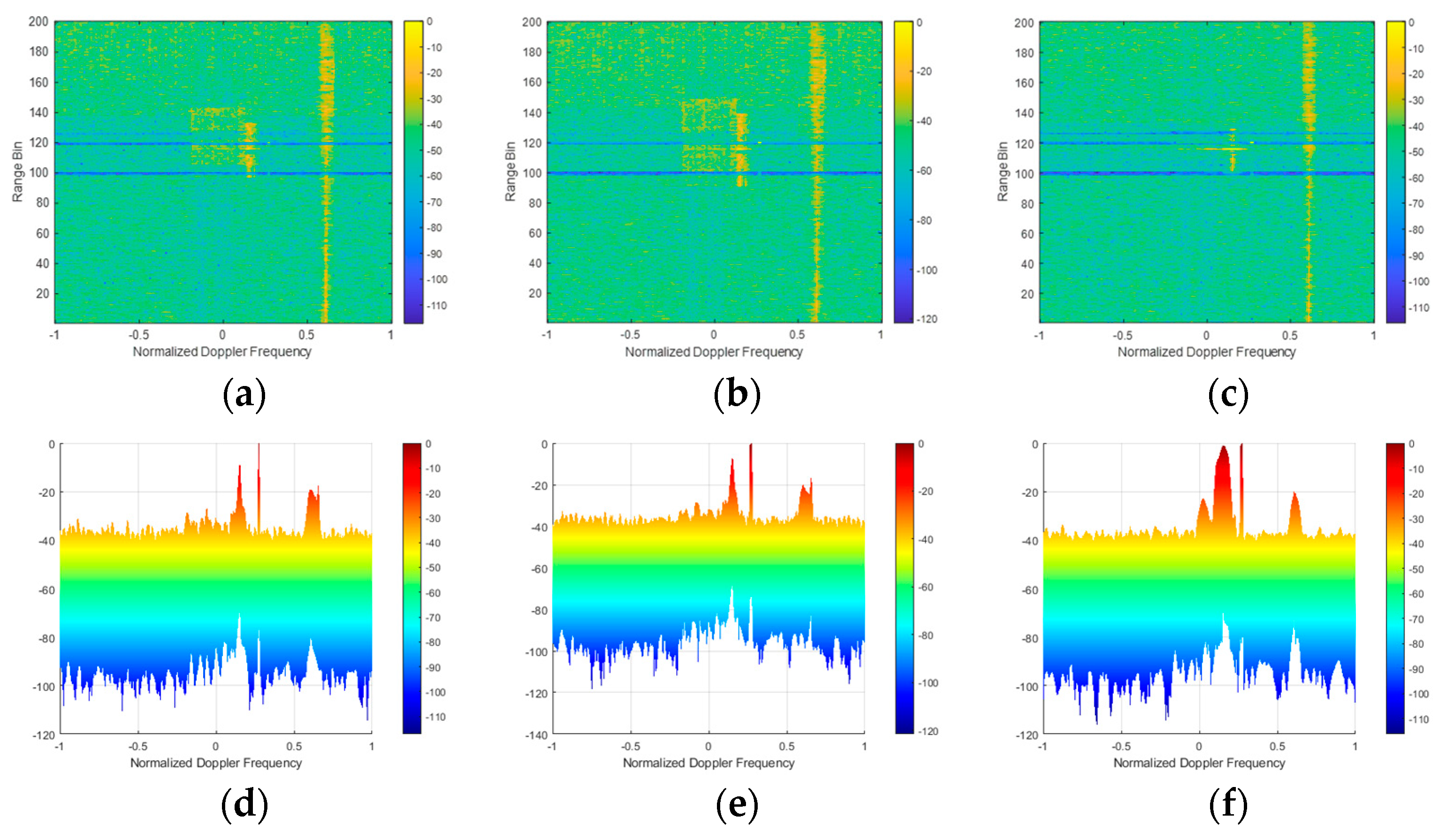
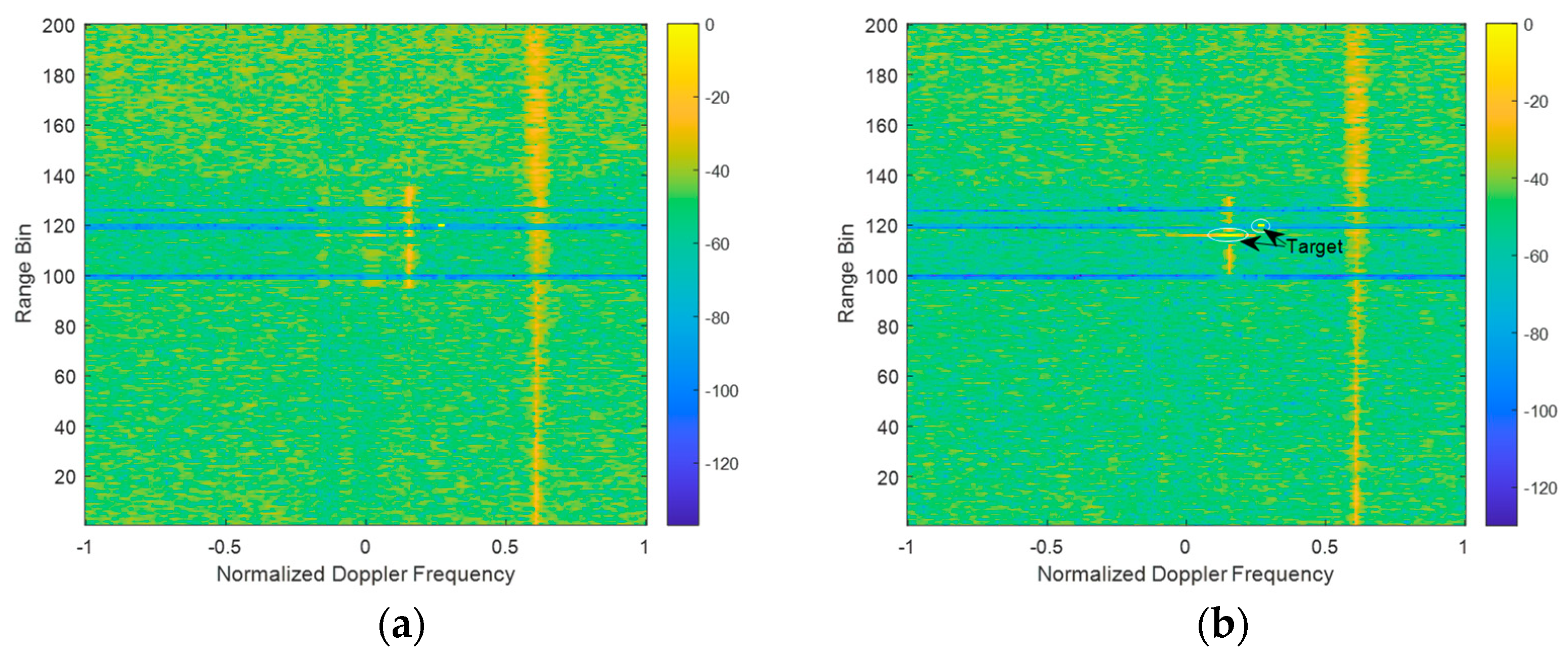
4.2. Multiple Wind Turbines

Here, we take into account that several wind turbines would impact the detection target, and that each wind turbine has a distinct speed. We assume that wind turbines one and two are located in the 99th–100th and 119th–120th equidistant rings, respectively, and operate at a speed of 12–13 r/min. Meanwhile, wind turbine three is located in the 126th–127th equidistant ring and operates at a speed of 15–17 r/min (speed at rated power).
Upon comparing Figure 18 and Figure 19b,c, and incorporating data from Figure 12, it becomes evident that by first screening out data samples containing WTC and subsequently applying OPTICS clustering for secondary clutter suppression, both target 1 and target 2 are discernible. Moreover, the energy levels of these targets are higher than those of ground clutter and background noise.
In order to fully demonstrate the performance of the clutter interference suppression algorithm based on space–time multi-beam joint OPTICS clustering, multiple sets of comparative experiments were designed for the STMB auxiliary channel selection strategy. The influences of the number of Doppler channels and the number of azimuth channels on the proposed interference clutter suppression algorithm are compared and explored when three, five, and seven auxiliary channels are selected, separately. The selection of six auxiliary channels is shown in Table 3.
In Figure 18 and Figure 19, the auxiliary channel is selected as mode 1; that is, the number of Doppler channels is three, and the number of azimuth channels is three. The performance comparison of the proposed interference clutter suppression algorithm under the remaining five auxiliary channel selection methods of scene 1 and scene 2 is given below.
From the output results of Figure 20, Figure 21, Figure 22 and Figure 23, the proposed clutter interference suppression algorithm under different STMB auxiliary channel selection methods can effectively suppress the interference while retaining the echo information of the target. With the increase in the number of Doppler channels, it shows better clutter and interference suppression performance, and the signal energy of target 2 is stronger, as shown in Figure 21d and Figure 23d. This shows that the STMB incorporating the OPTICS clustering algorithm requires more system freedom in the Doppler dimension than in the azimuth dimension.

5. Conclusions

The current system design employs GEO satellites as transmitters, effectively mitigating the issue of clutter broadening when the SABR system operates in a downward-looking mode. Nonetheless, the proliferation of wind farms poses new challenges for receiver radar due to increasing interference from wind turbine clutter (WTC). This interference also diminishes the effectiveness of space–time adaptive clutter suppression methods. This paper initially explores a precise space–time clutter model for the SABR system, considering the satellite’s launch orbit, Earth’s curved surface, and Earth’s rotation. Subsequently, we develop a geometric model of WTC and its space–time signal echo, considering WTC’s impact on the receiving platform. A comparative analysis of the clutter characteristics on the transmitter platform in GEO and MEO orbits reveals that WTC can cause detection blind spots at the radar’s receiving end. Based on these findings, we propose a dynamic clutter suppression algorithm that combines the 3D-STMB method with OPTICS clustering. Firstly, the STMB algorithm is utilized to screen the range gate samples containing WTC for the initial suppression of clutter. Then, OPTICS clustering is used to distinguish targets and clutter to achieve secondary clutter suppression, effectively suppressing the influence of WTC while retaining targets. Numerical simulation results have verified the effectiveness of this proposed clutter suppression method in WTC suppression.

Author Contributions

The contributions of the authors are as follows. Methodology and formulation, S.Z. (Shuo Zhang) and S.Z. (Shuangxi Zhang); software realization, N.Q. (Ning Qiao); validation and experiments, S.Z. (Shuo Zhang); writing and review, S.Z. (Shuo Zhang) and S.Z. (Shuangxi Zhang); funding acquisition, Q.D. and Y.W. All authors have read and agreed to the published version of the manuscript.

Funding

This research was funded by the National Natural Science Foundation of China under Grant 62271406, by the Aeronautical Science Foundation of China under Grant ASFC-20182053022 and by the Shanghai Aerospace Science and Technology Innovation Foundation under Grant SAST2022-045.

Data Availability Statement

Data are contained within the article.

Conflicts of Interest

The authors declare no conflicts of interest.

References

  1. Nohara, T.J. Design of a Space-Based Radar Signal Processor. IEEE Trans. Aerosp. Electron. Syst. 1998, 34, 366–377. [Google Scholar] [CrossRef]
  2. Davis, M.E.; Himed, B.; Zasada, D. Design of Large Space Based Radar for Multimode Surveillance. In Proceedings of the 2003 IEEE Radar Conference (Cat. No. 03CH37474), Huntsville, AL, USA, 8 May 2003; pp. 1–6. [Google Scholar]
  3. Hartnett, M.P.; Davis, M.E. Bistatic Surveillance Concept of Operations. In Proceedings of the 2001 IEEE Radar Conference (Cat. No. 01CH37200), Atlanta, GA, USA, 7 May 2001; pp. 75–80. [Google Scholar]
  4. Ma, J.; Yu, J.; Liang, G.; Sun, S.; Jiang, X.; Huang, P. Maneuvering Target Coherent Integration and Detection in PRI-Staggered Radar Systems. IEEE Geosci. Remote Sens. Lett. 2022, 19, 3105904. [Google Scholar] [CrossRef]
  5. Huang, P.; Xia, X.-G.; Wang, L.; Xu, H.; Liu, X.; Liao, G.; Jiang, X. Imaging and Relocation for Extended Ground Moving Targets in Multichannel SAR-GMTI Systems. IEEE Trans. Geosci. Remote Sens. 2022, 60, 3106906. [Google Scholar] [CrossRef]
  6. Griffiths, H.D. From a Different Perspective: Principles, Practice and Potential of Bistatic Radar. In Proceedings of the International Conference on Radar (IEEE Cat. No. 03EX695), Adelaide, SA, Australia, 3–5 September 2003; pp. 1–7. [Google Scholar]
  7. Zhang, Q.; Dong, Z.; Zhang, Y.; He, Z. GEO-UAV Bistatic Circular Synthetic Aperture Radar: Concepts and Technologies. In Proceedings of the 2016 IEEE International Geoscience and Remote Sensing Symposium (IGARSS), Beijing, China, 10–15 July 2016; pp. 4195–4198. [Google Scholar]
  8. Guttrich, G.L.; Sievers, W.E.; Tomljanovich, N.M. Wide Area Surveillance Concepts Based on Geosynchronous Illumination and Bistatic Unmanned Airborne Vehicles or Satellite Reception. In Proceedings of the 1997 IEEE National Radar Conference, Syracuse, NY, USA, 13–15 May 1997; pp. 126–131. [Google Scholar]
  9. Kong, F.; Zhang, Y.; Palmer, R. Wind Turbine Clutter Mitigation for Weather Radar by Adaptive Spectrum Processing. In Proceedings of the 2012 IEEE Radar Conference, Atlanta, GA, USA, 7–11 May 2012; pp. 471–474. [Google Scholar]
  10. Zhang, C.; Liu, H.; Long, T. Signal-to-Noise Ratio Analysis in Satellite-Airship Bistatic Space Based Radar. In Proceedings of the 2008 International Conference on Radar, Adelaide, Australia, 2–5 September 2008; pp. 434–439. [Google Scholar]
  11. Sun, Z.; Wu, J.; Pei, J.; Li, Z.; Huang, Y.; Yang, J. Inclined Geosynchronous Spaceborne–Airborne Bistatic SAR: Performance Analysis and Mission Design. IEEE Trans. Geosci. Remote Sens. 2016, 54, 343–357. [Google Scholar] [CrossRef]
  12. Rodriguez-Cassola, M.; Baumgartner, S.V.; Krieger, G.; Moreira, A. Bistatic TerraSAR-X/F-SAR Spaceborne–Airborne SAR Experiment: Description, Data Processing, and Results. IEEE Trans. Geosci. Remote Sens. 2010, 48, 781–794. [Google Scholar] [CrossRef]
  13. Espeter, T.; Walterscheid, I.; Klare, J.; Ender, J.H.G. Synchronization Techniques for the Bistatic Spaceborne/Airborne SAR Experiment with TerraSAR-X and PAMIR. In Proceedings of the 2007 IEEE International Geoscience and Remote Sensing Symposium, Barcelona, Spain, 23–28 July 2007; pp. 2160–2163. [Google Scholar]
  14. Cui, C.; Dong, X.; Hu, C. Performance Analysis and Configuration Design of Geosynchronous Spaceborne-Airborne Bistatic Moving Target Indication System. In Proceedings of the IGARSS 2020—2020 IEEE International Geoscience and Remote Sensing Symposium, Waikoloa, HI, USA, 26 September–2 October 2020; pp. 6559–6562. [Google Scholar]
  15. Ding, T.; Zhang, J.; Tang, S.; Zhang, L.; Li, Y. A Novel Iterative Inner-Pulse Integration Target Detection Method for Bistatic Radar. IEEE Trans. Geosci. Remote Sens. 2022, 60, 3186012. [Google Scholar] [CrossRef]
  16. Zhang, J.; Ding, T.; Zhang, L. Longtime Coherent Integration Algorithm for High-Speed Maneuvering Target Detection Using Space-Based Bistatic Radar. IEEE Trans. Geosci. Remote Sens. 2022, 60, 3038199. [Google Scholar] [CrossRef]
  17. Wang, Z.; Wang, Y.; Xing, M.; Sun, G.-C.; Zhang, S.; Xiang, J. A Novel Two-Step Scheme Based on Joint GO-DPCA and Local STAP in Image Domain for Multichannel SAR-GMTI. IEEE J. Sel. Top. Appl. Earth Obs. Remote Sens. 2021, 14, 8259–8272. [Google Scholar] [CrossRef]
  18. Wu, J.; Sun, Z.; Huang, Y.; Yang, J.; Lv, Y.; Wang, Z. Geosynchronous Spaceborne-Airborne Bistatic SAR: Potentials and Prospects. In Proceedings of the 2015 IEEE Radar Conference (RadarCon), Arlington, VA, USA, 10–15 May 2015; pp. 1172–1176. [Google Scholar]
  19. Zeng, T.; Hu, C.; Wu, L.; Liu, F.; Tian, W.; Zhu, M.; Long, T. Extended NLCS Algorithm of BiSAR Systems with a Squinted Transmitter and a Fixed Receiver: Theory and Experimental Confirmation. IEEE Trans. Geosci. Remote Sens. 2013, 51, 5019–5030. [Google Scholar] [CrossRef]
  20. Wu, J.; Li, Z.; Huang, Y.; Yang, J.; Liu, Q.H. Omega-K Imaging Algorithm for One-Stationary Bistatic SAR. IEEE Trans. Aerosp. Electron. Syst. 2014, 50, 33–52. [Google Scholar] [CrossRef]
  21. Huang, P.; Zou, Z.; Xia, X.-G.; Liu, X.; Liao, G.; Xin, Z. Multichannel Sea Clutter Modeling for Spaceborne Early Warning Radar and Clutter Suppression Performance Analysis. IEEE Trans. Geosci. Remote Sens. 2021, 59, 8349–8366. [Google Scholar] [CrossRef]
  22. Huang, P.; Zou, Z.; Xia, X.-G.; Liu, X.; Liao, G. A Novel Dimension-Reduced Space–Time Adaptive Processing Algorithm for Spaceborne Multichannel Surveillance Radar Systems Based on Spatial–Temporal 2-D Sliding Window. IEEE Trans. Geosci. Remote Sens. 2022, 60, 3144668. [Google Scholar] [CrossRef]
  23. Li, Z.; Ye, H.; Liu, Z.; Sun, Z.; An, H.; Wu, J.; Yang, J. Bistatic SAR Clutter-Ridge Matched STAP Method for Nonstationary Clutter Suppression. IEEE Trans. Geosci. Remote Sens. 2022, 60, 3125043. [Google Scholar] [CrossRef]
  24. Yang, X.; Wang, W.; Wang, Y.; Duan, K. Clutter Modeling and Analysis for Bistatic Space-Based Early Warning Radar with GEO Transmitter and LEO Receiver. In Proceedings of the 2023 IEEE International Radar Conference, Sydney, Australia, 6–10 November 2023; pp. 1–6. [Google Scholar]
  25. Huang, P.; Yang, H.; Xia, X.-G.; Zou, Z.; Liu, X.; Liao, G. A Novel Sea Clutter Rejection Algorithm for Spaceborne Multichannel Radar Systems. IEEE Trans. Geosci. Remote Sens. 2022, 60, 3204324. [Google Scholar] [CrossRef]
  26. Huang, P.; Yang, H.; Zou, Z.; Xia, X.-G.; Liao, G.; Zhang, Y. Range-Ambiguous Sea Clutter Suppression for Multichannel Spaceborne Radar Applications Via Alternating APC Processing. IEEE Trans. Aerosp. Electron. Syst. 2023, 59, 6954–6970. [Google Scholar] [CrossRef]
  27. Li, H.; Tang, J.; Peng, Y. Effects of Geometry on Clutter Characteristics of Hybrid Bistatic Space Based Radar. In Proceedings of the 2006 CIE International Conference on Radar, Shanghai, China, 16–19 October 2006; pp. 1–4. [Google Scholar]
  28. Li, H.; Tang, J.; Peng, Y. Clutter Modeling and Characteristics Analysis for Bistatic SBR. In Proceedings of the 2007 IEEE Radar Conference, Waltham, MA, USA, 17–20 April 2007; pp. 513–517. [Google Scholar]
  29. Kan, Q.; Xu, J.; Liao, G.; Wang, K.; Xu, Y. Clutter Compensation for Space-Air Bistatic Radar Based on Unitary Subspace Transformation. In Proceedings of the 2023 IEEE International Radar Conference (RADAR), Sydney, Australia, 6–10 November 2023; pp. 1–5. [Google Scholar]
  30. Kan, Q.; Xu, J.; Liao, G.; Zhang, Y.; Xu, Y.; Wang, W. Clutter Characteristics Analysis and Range-Dependence Compensation for Space-Air Bistatic Radar. IEEE Trans. Geosci. Remote Sens. 2023, 62, 5101615. [Google Scholar] [CrossRef]
  31. Cui, C.; Dong, X.; Chen, Z.; Hu, C.; Tian, W. A Long-Time Coherent Integration STAP for GEO Spaceborne-Airborne Bistatic SAR. Remote Sens. 2022, 14, 593. [Google Scholar] [CrossRef]
  32. Li, B.; Shen, Y.; Li, W. The Seamless Model for Three-Dimensional Datum Transformation. Sci. China Earth Sci. 2012, 55, 2099–2108. [Google Scholar] [CrossRef]
  33. Wang, Q.; Xue, B.; Hu, X.; Wu, G.; Zhao, W. Robust Space–Time Joint Sparse Processing Method with Airborne Active Array for Severely Inhomogeneous Clutter Suppression. Remote Sens. 2022, 14, 2647. [Google Scholar] [CrossRef]
  34. Klemm, R. Comparison between Monostatic and Bistatic Antenna Configurations for STAP. IEEE Trans. Aerosp. Electron. Syst. 2000, 36, 596–608. [Google Scholar] [CrossRef]
  35. Zhang, S.; Wang, T.; Liu, C.; Ren, B. A Fast IAA–Based SR–STAP Method for Airborne Radar. Remote Sens. 2024, 16, 1388. [Google Scholar] [CrossRef]
  36. Reed, I.S.; Mallett, J.D.; Brennan, L.E. Rapid Convergence Rate in Adaptive Arrays. IEEE Trans. Aerosp. Electron. Syst. 1974, AES-10, 853–863. [Google Scholar] [CrossRef]
  37. Liu, J.; Liao, G.; Zeng, C.; Tao, H.; Xu, J.; Zhu, S.; Juwono, F.H. Reweighted Extreme Learning Machine-Based Clutter Suppression and Range Compensation Algorithm for Non-Side-Looking Airborne Radar. Remote Sens. 2024, 16, 1093. [Google Scholar] [CrossRef]
  38. Qiao, N.; Zhang, S.; Zhang, S.; Du, Q.; Wang, Y. A Novel Non-Stationary Clutter Suppression Approach for Space-Based Early Warning Radar Using an Interpulse Multi-Frequency Mode. Remote Sens. 2024, 16, 314. [Google Scholar] [CrossRef]
  39. Wang, Z.; Chen, W.; Zhang, T.; Xing, M.; Wang, Y. Improved Dimension-Reduced Structures of 3D-STAP on Nonstationary Clutter Suppression for Space-Based Early Warning Radar. Remote Sens. 2022, 14, 4011. [Google Scholar] [CrossRef]
  40. Zhang, T.; Wang, Z.; Xing, M.; Zhang, S.; Wang, Y. Research on Multi-Domain Dimensionality Reduction Joint Adaptive Processing Method for Range Ambiguous Clutter of FDA-Phase-MIMO Space-Based Early Warning Radar. Remote Sens. 2022, 14, 5536. [Google Scholar] [CrossRef]
  41. He, W.; Zhai, Q.; Wang, X.; Wu, R. Wind Turbine Clutter Detection and Mitigation in Scanning ATC Surveillance Radar. Acta Aeronaut. Et Astronaut. Sin. 2016, 37, 1316–1326. [Google Scholar]
  42. Zhang, R.; Li, G.; Zhang, Y.D. Micro-Doppler Interference Removal via Histogram Analysis in Time-Frequency Domain. IEEE Trans. Aerosp. Electron. Syst. 2016, 52, 755–768. [Google Scholar] [CrossRef]
  43. Rashid, L.; Brown, A. Partial Treatment of Wind Turbine Blades with Radar Absorbing Materials (RAM) for RCS Reduction. In Proceedings of the Fourth European Conference on Antennas and Propagation, Barcelona, Spain, 12–16 April 2010; pp. 1–5. [Google Scholar]
  44. Karabayir, O.; Unal, M.; Coskun, A.F.; Yucedag, S.M.; Saynak, U.; Bati, B.; Biyik, M.; Bati, O.; Serim, H.A.; Kent, S. CLEAN Based Wind Turbine Clutter Mitigation Approach for Pulse-Doppler Radars. In Proceedings of the 2015 IEEE Radar Conference (RadarCon), Arlington, VA, USA, 10–15 May 2015; pp. 1541–1544. [Google Scholar]
  45. Wu, R.B.; Mao, J.; Wang, X.L.; Jia, Q.Q. Target Detection of Primary Surveillance Radar in Wind Farm Clutter. J. Electron. Inf. Technol. 2013, 35, 754–758. [Google Scholar] [CrossRef]
  46. Uysal, F.; Pillai, U.; Selesnick, I.; Himed, B. Signal Decomposition for Wind Turbine Clutter Mitigation. In Proceedings of the 2014 IEEE Radar Conference, Cincinnati, OH, USA, 19–23 May 2014; pp. 0060–0063. [Google Scholar]
  47. Naqvi, A.; Ling, H. Signal Filtering Technique to Remove Doppler Clutter Caused by Wind Turbines. Microw. Opt. Technol. Lett. 2012, 54, 1455–1460. [Google Scholar] [CrossRef]
  48. Hu, X.; Tan, X.; Qu, Z.; Luo, Y.; Chi, P. Wind Turbine Clutter Suppression Method Based on Dynamic Reconstruction. Acta Aeronaut. Et Astronaut. Sin. 2020, 41, 323269. [Google Scholar]
  49. Pan, Y.; Rao, Y.; Chen, Y.; Cheng, F. Wind Turbine Clutter Suppression Method Based on Reference Signal Correction for Passive Radar. Syst. Eng. Electron. 2023, 45, 2446–2454. [Google Scholar]
  50. Zulch, P.; Davis, M.; Adzima, L.; Hancock, R.; Theis, S. The Earth Rotation Effect on a LEO L-Band GMTI SBR and Mitigation Strategies. In Proceedings of the 2004 IEEE Radar Conference (IEEE Cat. No. 04CH37509), Philadelphia, PA, USA, 29 April 2004; pp. 27–32. [Google Scholar]
  51. Pillai, S.U.; Li, K.Y.; Himed, B. Space Based Radar: Theory & Applications; McGraw-Hill Professional Publishing: New York, NY, USA, 2007; pp. 77–137. [Google Scholar]
  52. Wang, Y.; Chen, J. Robust STAP Approach in Nonhomogeneous Clutter Environments. In Proceedings of the 2001 CIE International Conference on Radar Proceedings (Cat No. 01TH8559), Beijing, China, 15–18 October 2001; pp. 753–757. [Google Scholar]
  53. Ankerst, M.; Breunig, M.M.; Kriegel, H.-P.; Sander, J. OPTICS: Ordering Points to Identify the Clustering Structure. SIGMOD Rec. 1999, 28, 49–60. [Google Scholar] [CrossRef]
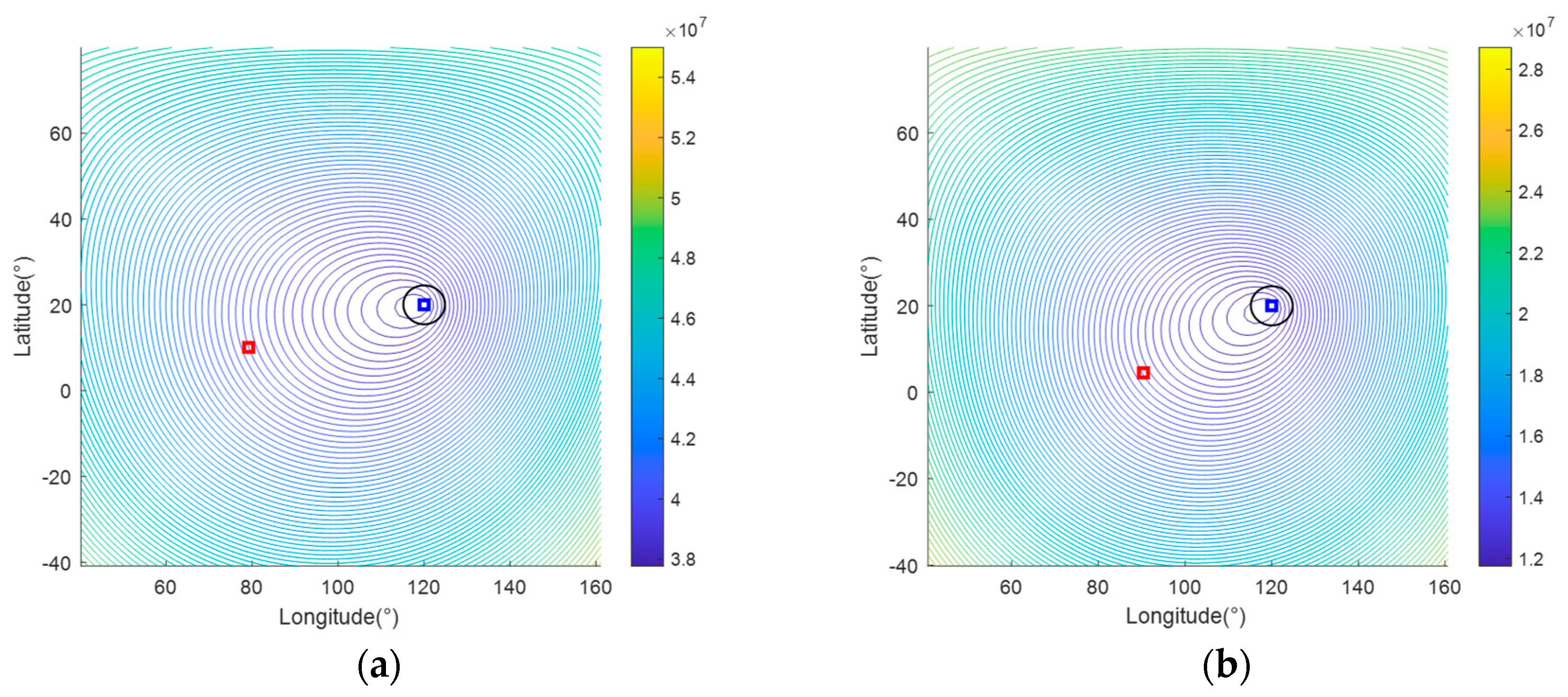
Figure 1. SABR geometry.
Remotesensing 16 02674 g001
Figure 2. Auxiliary coordinate systems O-XYZ and M-XYZ′.
Remotesensing 16 02674 g002
Figure 3. Schematic diagram of conversion from coordinate system O-XYZ to Earth-fixed coordinate system O-XeYeZe.
Remotesensing 16 02674 g003
Figure 4. Description of satellite orbits and satellite velocity components.
Remotesensing 16 02674 g004
Figure 5. Clutter iso-range rings: (a) GEO; (b) MEO.
Remotesensing 16 02674 g005
Figure 6. Iso-Doppler traces: (a) GEO; (b) MEO.
Remotesensing 16 02674 g006
Figure 7. Schematic diagram illustrating the geometric relationship between the array of receiving platforms and the movement of the windmill.
Remotesensing 16 02674 g007
Figure 8. At a particular moment, the geometric relationship between each fan blade and the receiving platform: (a) vector representation of linear velocity; (b) fan blade three is located in the main beam.
Remotesensing 16 02674 g008
Figure 9. Range-Doppler power spectra before and after the impact of WTC (Scenario 1—upper, Scenario 2—lower): (a,d) WTC is not considered; (b,e) WTC is considered; (c,f) three-dimensional top views of the distance gates where WTC is located.
Remotesensing 16 02674 g009
Figure 10. Processing flow chart of the proposed method.
Remotesensing 16 02674 g010
Figure 11. STMB-STAP algorithm.
Remotesensing 16 02674 g011
Figure 12. RD comparison diagrams of STMB-STAP output before and after sample selection: (a,b) unscreened WTC sample distance gates; (c,d) screening WTC samples.
Remotesensing 16 02674 g012
Figure 13. OPTICS clustering: (a) schematic diagram of core concepts; (b) reachability plots for containing echo data of WTC and target.
Remotesensing 16 02674 g013
Figure 14. OPTICS clustering flow chart.
Remotesensing 16 02674 g014
Figure 15. Clutter range-Doppler spectra under the influence of WTC (Scenario 1—upper, Scenario 2—lower): (a,c) range-Doppler power spectra; (b,d) clutter suppression output results.
Remotesensing 16 02674 g015
Figure 16. WTC clutter suppression based on orthogonal subspace (Scenario 1—upper, Scenario 2—lower): (a,c) range-Doppler power spectra; (b,d) three-dimensional side views of clutter suppression output results.
Remotesensing 16 02674 g016
Figure 17. Clutter range-Doppler spectra after clustering processing (Scenario 1—upper, Scenario 2—lower): (a,c) range-Doppler power spectra; (b,d) three-dimensional side views of clutter suppression output results.
Remotesensing 16 02674 g017
Figure 18. Scenario 1 clutter range-Doppler spectra: (a) after STMB clutter processing; (b) after clustering processing; (c) three-dimensional side view of clutter suppression output results.
Remotesensing 16 02674 g018
Figure 19. Scenario 2 clutter range–Doppler spectra: (a) after STMB clutter processing; (b) after clustering processing; (c) three-dimensional side view of clutter suppression output results.
Remotesensing 16 02674 g019
Figure 20. Scenario 1 clutter range-Doppler spectra: (a) Select method 2; (b) Select method 3; (c) Select method 4; (df) are the three-dimensional side views of the corresponding clutter suppression output results.
Remotesensing 16 02674 g020
Figure 21. Scenario 1 Clutter range-Doppler spectra: (a) Select method 5; (b) Select method 6; (c,d) are the three-dimensional side views of the corresponding clutter suppression output results.
Remotesensing 16 02674 g021aRemotesensing 16 02674 g021b
Figure 22. Scenario 2 clutter range-Doppler spectra: (a) Select method 2; (b) Select method 3; (c) Select method 4; (df) are the three-dimensional side views of the corresponding clutter suppression output results.
Remotesensing 16 02674 g022
Figure 23. Scenario 2 clutter range-Doppler spectra: (a) Select method 5; (b) Select method 6; (c,d) are the three-dimensional side views of the corresponding clutter suppression output results.
Remotesensing 16 02674 g023aRemotesensing 16 02674 g023b
Table 1. Platform parameters.
TypeParametersValues and Units
GEO satelliteMEO satellite
TransmitterAltitude35,784 km10,000 km
Velocity3.07 km/s4.93 km/s
Longitude and latitude(79.21°E,10.08°N)(90.4°E, 4.47°N)
Orbit inclination15.31°
ReceiverAltitude20 km
Velocity125 m/s
Longitude and latitude(120°E, 20°N)
Table 2. Receiving platform and radar system parameters.
ParametersSymbolValue
Number of column channelsN16 (subarray synthesis)
Number of row channelsM14
Carrier frequencyfc1.25 GHz
Channel spacingd0.24 m
Pulse repetition frequencyfr2 kHz
Number of pulses in a CPIK64
Range ring widthdR60 m
Clutter-to-noise ratioCNR45 dB
Table 3. Auxiliary channel selection method.
Doppler Dimension and Azimuth Dimension ChannelsSelect Method
3-31
3-52
3-73
5-34
5-55
7-36
Disclaimer/Publisher’s Note: The statements, opinions and data contained in all publications are solely those of the individual author(s) and contributor(s) and not of MDPI and/or the editor(s). MDPI and/or the editor(s) disclaim responsibility for any injury to people or property resulting from any ideas, methods, instructions or products referred to in the content.

