
Evaluating Coseismic Landslide Susceptibility Following the 2022 Luding Earthquake: A Comparative Analysis of Six Displacement Regression Models Integrating Epicentral and Seismogenic Fault Distances within the Permanent-Displacement Framework

Abstract
:1. Introduction
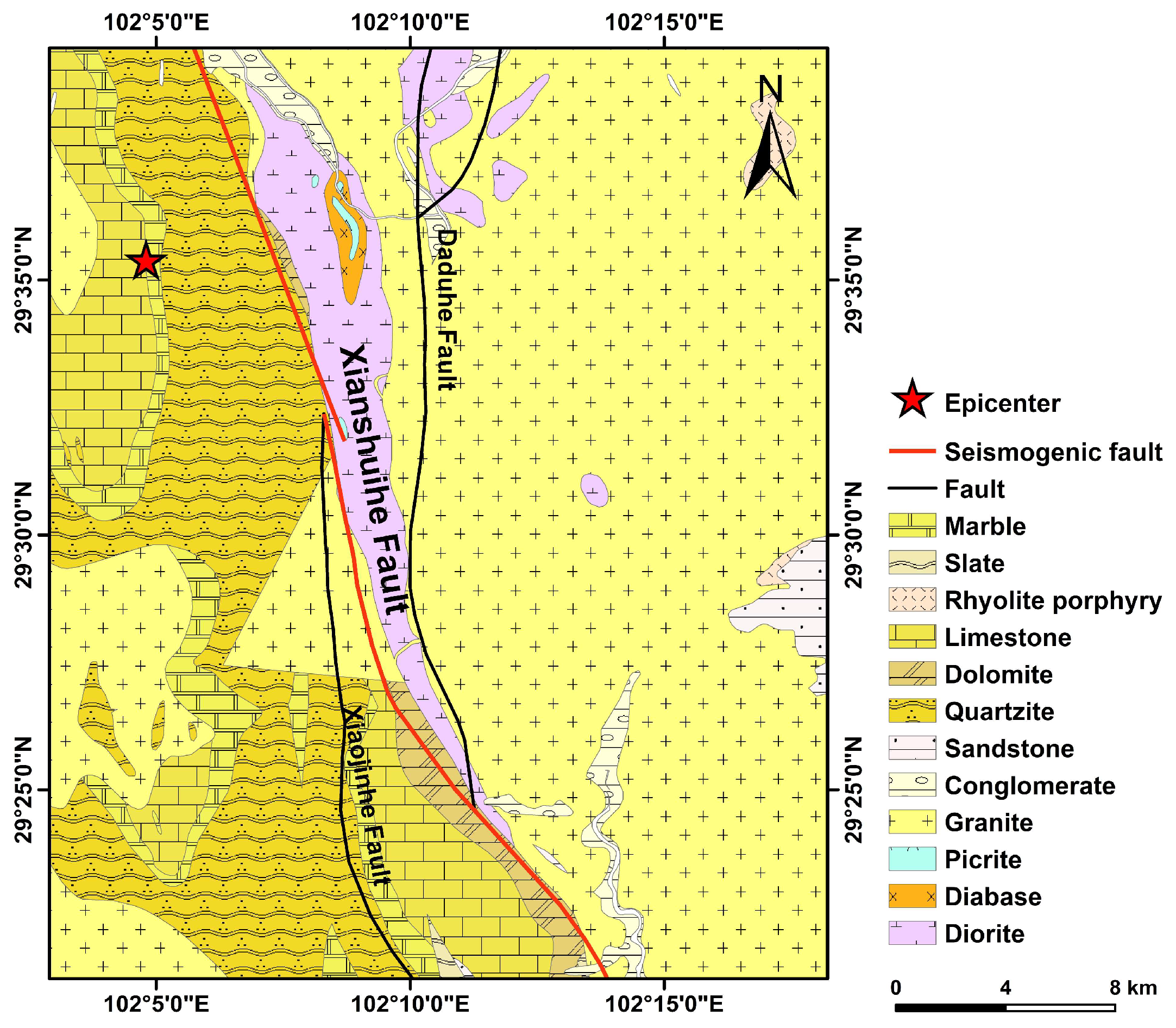
2. Study Area
3. Materials and Methodology
3.1. Sources of Data
3.2. Inventory of the Landslides Induced by the 2022 Luding Earthquake
3.3. Methodology
4. Results and Analysis
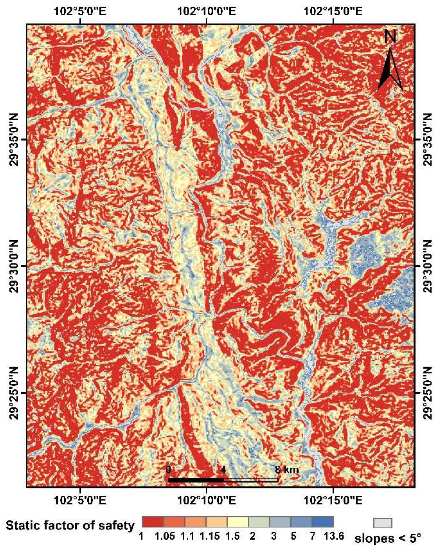
4.1. Static Factor-of-Safety Map
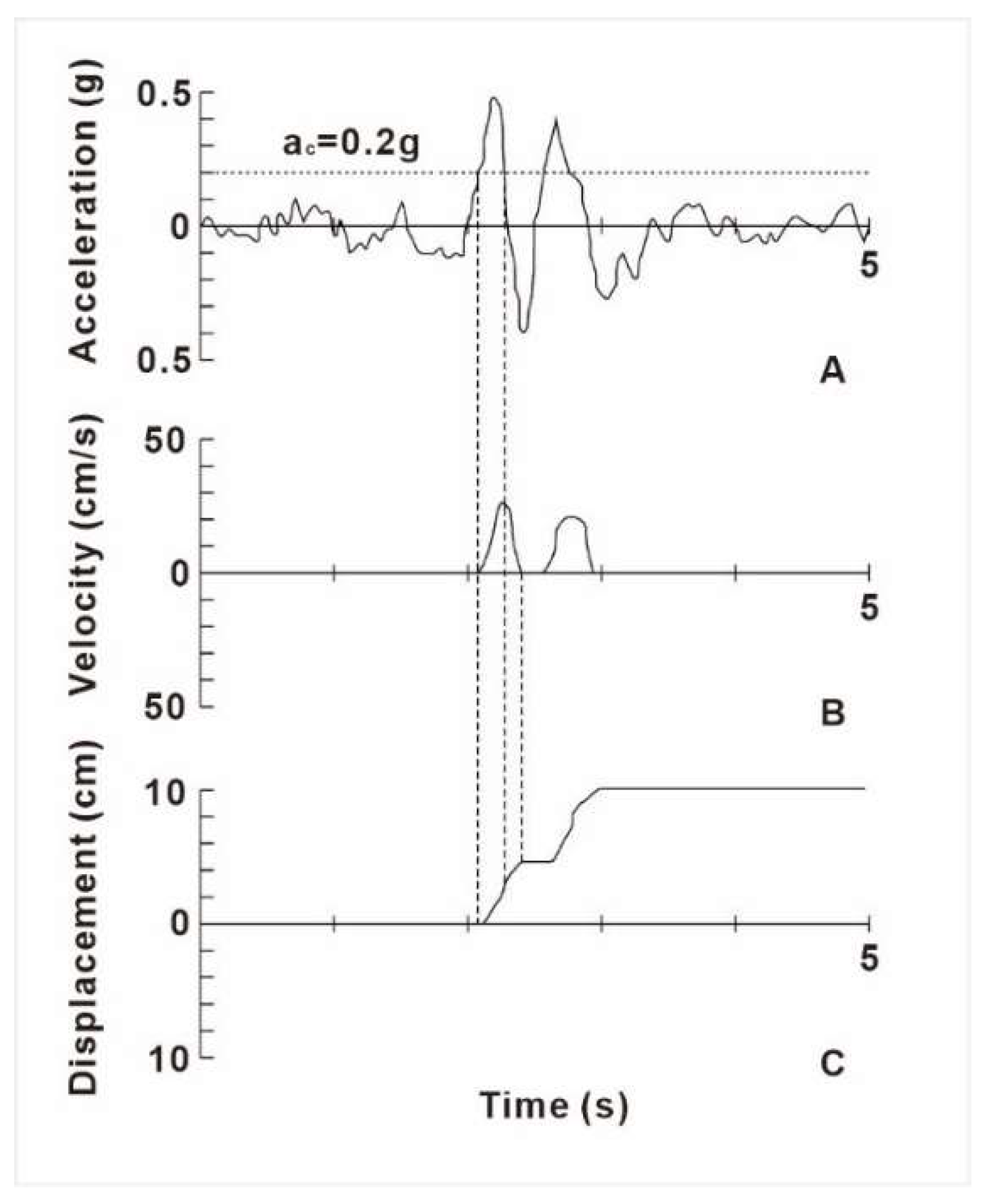
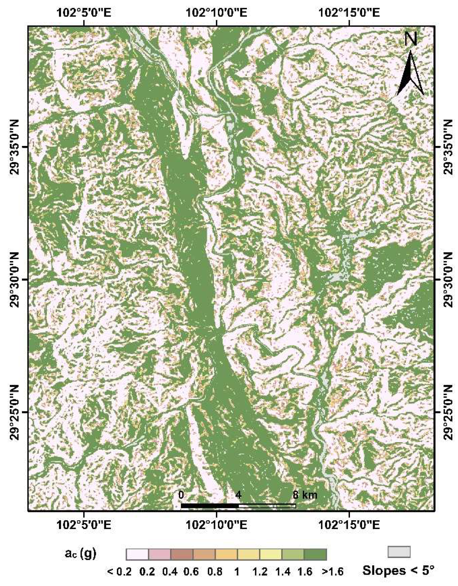
4.2. Critical Acceleration Map
4.3. Predicted Displacement Map
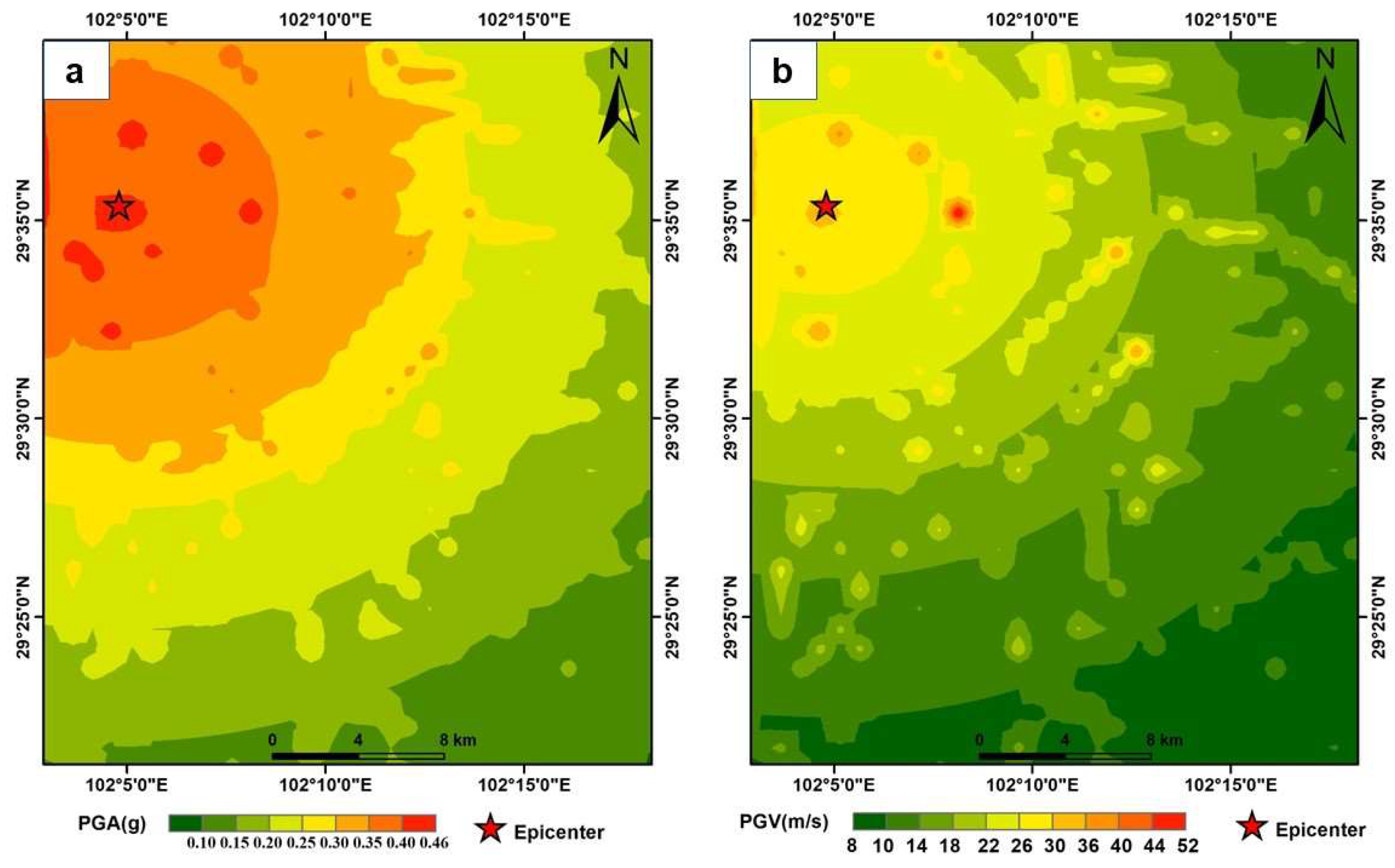
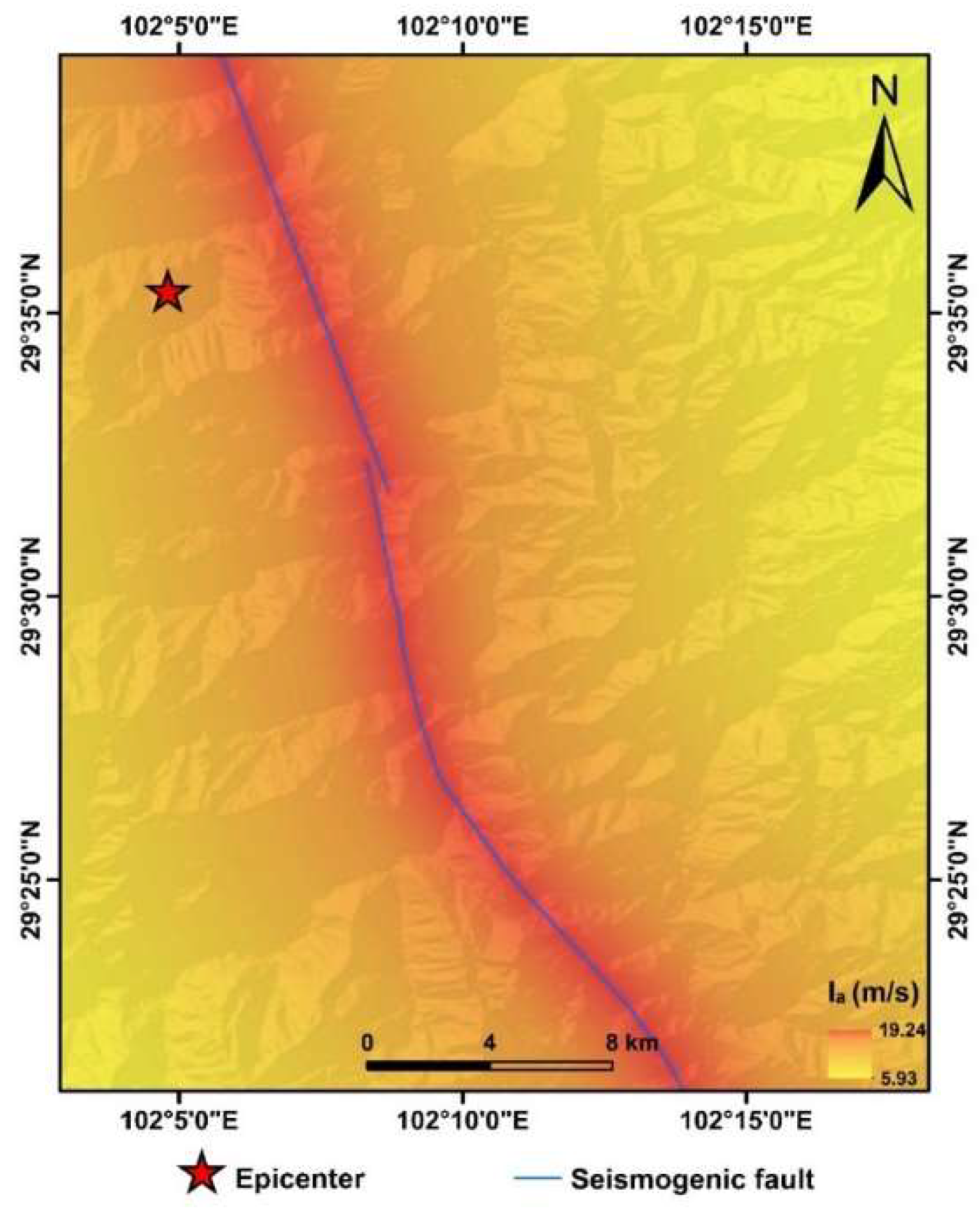
4.3.1. Seismic Motion Map
4.3.2. Newmark Displacement Map
4.4. Comparative Analysis of Regression Models
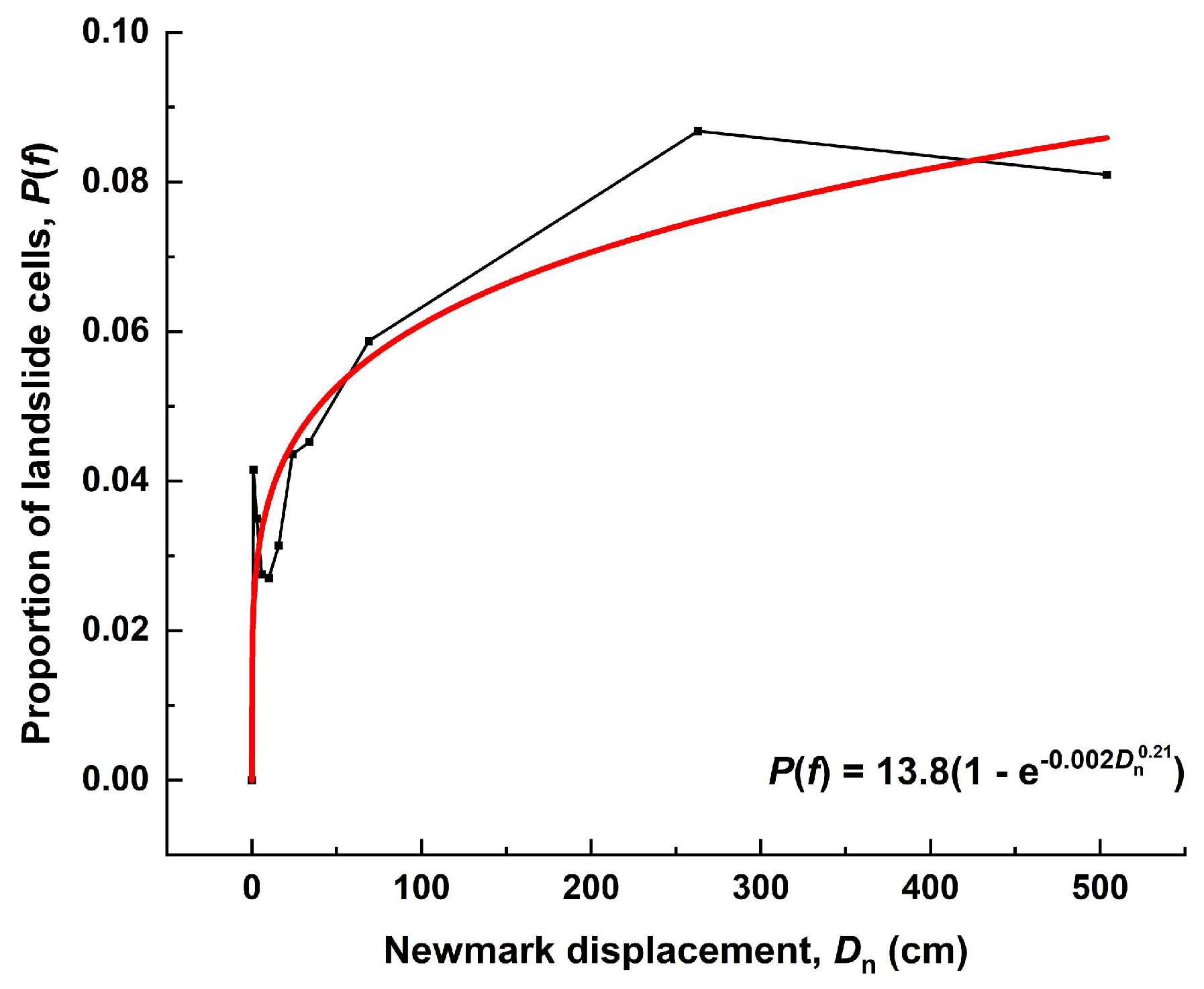
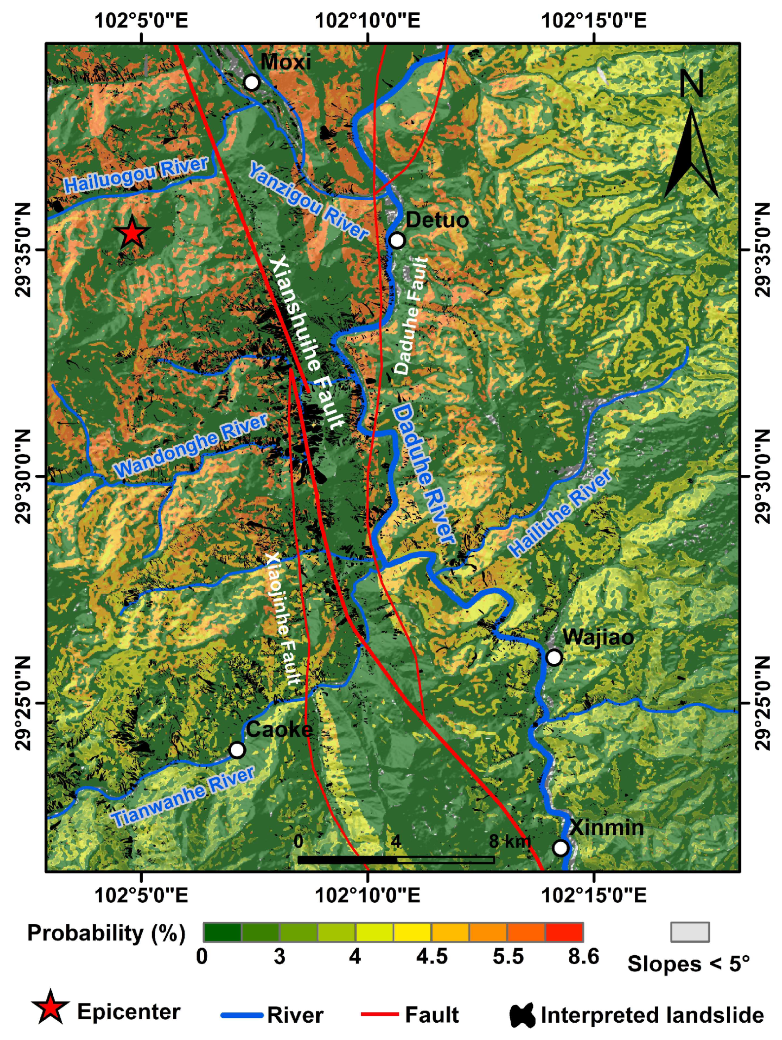
4.5. Spatial Probability of Coseismic Landslides
5. Discussion
6. Conclusions
Author Contributions
Funding
Data Availability Statement
Acknowledgments
Conflicts of Interest
References
- Keefer, D.K. Landslides caused by earthquakes. Geol. Soc. Am. Bull. 1984, 95, 406–421. [Google Scholar] [CrossRef]
- Fan, X.M.; Wang, X.; Dai, L.X.; Fang, C.Y.; Deng, Y.; Zou, C.B.; Tang, M.G.; Wei, Z.L.; Dou, X.Y.; Zhang, J.; et al. Characteristics and spatial distribution pattern of M S 6.8 Luding earthquake occurred on September 5, 2022. J. Eng. Geol. 2022, 30, 1504–1516. [Google Scholar]
- Sun, Y.K.; Mou, H.C.; Yao, B.K. Slope Stability Analysis; Science Press: Beijing, China, 1988. [Google Scholar]
- Parise, M.; Jibson, R.W. A seismic landslide susceptibility rating of geologic units based on analysis of characteristics of landslides triggered by the 17 January, 1994 Northridge, California earthquake. Eng. Geol. 2000, 58, 251–270. [Google Scholar] [CrossRef]
- Marzorati, S.; Luzi, L.; De, A.M. Rock falls induced by earthquakes: A statistical approach. Soil Dyn. Earthq. Eng. 2002, 22, 565–577. [Google Scholar] [CrossRef]
- Wang, Y.Q.; Gao, Y.P.; Xin, H.B. A research on prediction of seismic stability of slopes by grey clustering method. Ind. Constr. 2002, 32, 44–47. [Google Scholar]
- Miles, S.B.; Keefer, D.K. Evaluation of CAMEL—Comprehensive areal model of earthquake-induced landslides. Eng. Geol. 2009, 104, 1–15. [Google Scholar]
- Terzaghi, K. Mechanism of Landslides. In Application of Geology to Engineering Practice; Paige, S., Ed.; Geological Society of America: Boulder, CO, USA, 1950. [Google Scholar]
- Seed, H.B. Stability of Earth and Rockfill Dams during Earthquakes; Wiley (John) and Sons: Hoboken, NJ, USA, 1973. [Google Scholar]
- Jibson, R.W. Methods for assessing the stability of slopes during earthquakes—A retrospective. Eng. Geol. 2011, 122, 43–50. [Google Scholar]
- Wu, X.Y.; Law, K.T.; Selvadural, A.S. Examination of the pseudo-static limit equilibrium method for dynamic stability analysis of slopes. In Proceedings of the 44th Canadian Geotechnical Conference, Calgary, AB, Canada, 29 September–2 October 1991; pp. 1961–1968. [Google Scholar]
- Ling, H.I.; Cheng, A.H. Rock sliding induced by seismic force. Int. J. Rock Mech. Min. Sci. 1997, 34, 1021–1029. [Google Scholar]
- Clough, R.W.; Chopra, A.K. Earthquake stress analysis in earth dams. J. Eng. Mech. Div. 1966, 92, 197–211. [Google Scholar]
- Zang, M.D. A probabilistic Framework for Mapping Hazards of Coseismic Landslides; University of Chinese Academy of Sciences: Beijing, China, 2019. [Google Scholar]
- Newmark, N.M. Effects of earthquakes on dams and embankments. Geotechnique 1965, 15, 139–160. [Google Scholar]
- Jibson, R.W.; Harp, E.L.; Michael, J.A. A Method for Producing Digital Probabilistic Seismic Landslide Hazard Maps: An Example from the Los Angeles, California, Area; US Department of the Interior, US Geological Survey: Washington, DC, USA, 1998.
- Jibson, R.W.; Harp, E.L.; Michael, J.A. A method for producing digital probabilistic seismic landslide hazard maps. Eng. Geol. 2000, 58, 271–289. [Google Scholar]
- Wang, T.; Wu, S.R.; Shi, J.S.; Xin, P. Case study on rapid assessment of regional seismic landslide hazard based on simplified Newmark displacement model: Wenchuan Ms 8.0 earthquake. J. Eng. Geol. 2013, 21, 16–24. [Google Scholar]
- Chen, X.L.; Yuan, R.M.; Yu, L. Applying the Newmark’s model to the assessment of earthquake-triggered landslides during the Lushan earthquake. Seismol. Geol. 2013, 35, 661–670. [Google Scholar]
- Chen, X.L.; Liu, C.; Wang, M. A method for quick assessment of earthquake-triggered landslide hazards: A case study of the Mw6. 1 2014 Ludian, China earthquake. Bull. Eng. Geol. Environ. 2019, 78, 2449–2458. [Google Scholar] [CrossRef]
- Zang, M.D.; Qi, S.W.; Zou, Y.; Sheng, Z.P.; Blanca, S.Z. An improved method of Newmark analysis for mapping hazards of coseismic landslides. Nat. Hazards Earth Syst. Sci. 2020, 20, 713–726. [Google Scholar] [CrossRef]
- Liu, J.M.; Wang, T.; DU, J.J.; Chen, K.; Huang, J.H.; Wang, H.J.; Ruan, Q.Q.; Feng, F. Emergency rapid assessment of landslides induced by the Luding MS6.8 earthquake in Sichuan of China. Hydrogeol. Eng. Geol. 2023, 50, 84–94. [Google Scholar]
- Ambraseys, N.N.; Menu, J.M. Earthquake-induced ground displacements. Earthq. Eng. Struct. Dyn. 1988, 16, 985–1006. [Google Scholar]
- Jibson, R.W. Predicting earthquake-induced landslide displacements using Newmark’s sliding block analysis. Transp. Res. Rec. 1993, 1411, 9–17. [Google Scholar]
- Jibson, R.W. Regression models for estimating coseismic landslide displacement. Eng. Geol. 2007, 91, 209–218. [Google Scholar]
- Saygili, G.; Rathje, E.M. Empirical predictive models for earthquake-induced sliding displacements of slopes. J. Geotech. Geoenviron. Eng. 2008, 134, 790–803. [Google Scholar]
- Rathje, E.M.; Saygili, G. Probabilistic assessment of earthquake-induced sliding displacements of natural slopes. Bull. N. Z. Soc. Earthq. Eng. 2009, 42, 18–27. [Google Scholar] [CrossRef]
- Xu, G.X.; Yao, L.K.; Li, C.H.; Wang, X.F. Predictive models for permanent displacement of slopes based on recorded strong-motion data of Wenchuan earthquake. Chin. J. Geotech. Eng. 2012, 34, 1131–1136. [Google Scholar]
- Jin, J.L.; Wang, Y.; Gao, D.; Yuan, R.M.; Yang, X.Y. New evaluation models of Newmark displacement for Southwest China. Bull. Seismol. Soc. Am. 2018, 108, 2221–2236. [Google Scholar]
- Yang, Z.; Dai, D.; Zhang, Y.; Zhang, X.M.; Liu, J. Rupture process and aftershock focal mechanisms of the 2022 M6. 8 Luding earthquake in Sichuan. Earthq. Sci. 2022, 35, 474–484. [Google Scholar]
- Zhang, P.Z. Current Tectonic Deformation, Strain Distribution and Deep Dynamic Process in the Western Sichuan of the Eastern Margin of the Tibetan Plateau. Sci. China (Ser. D) 2008, 38, 1041–1056. [Google Scholar]
- Bai, M.K.; Chevalier, M.L.; Li, H.B.; Pan, J.W.; Wu, Q.; Wang, S.G.; Liu, F.C.; Jiao, L.Q.; Zhang, J.J.; Zhang, L.; et al. Late Quaternary slip rate and earthquake hazard along the Qianning segment, Xianshuihe fault. Acta Geol. Sin. 2022, 96, 2312–2332. [Google Scholar]
- Wang, X.Y.; Wang, D.W. Relationships between the Wenchuan earthquake-induced landslide and peak ground velocity, Sichuan, China. Geol. Bull. China 2011, 30, 159–165. [Google Scholar]
- Shao, X.Y.; Ma, S.Y.; Xu, C.; Xie, C.C.; Li, T.; Huang, Y.D.; Huang, Y.; Xiao, Z.K. Landslides triggered by the 2022 Ms. 6.8 Luding strike-slip earthquake: An update. Eng. Geol. 2024, 335, 107536. [Google Scholar]
- Xie, J.J.; Wen, Z.P.; Gao, M.T.; Hu, J.X.; He, S.L. Characteristics of near-fault vertical and horizontal ground motion from the 2008 Wenchuan earthquake. Chin. J. Geophys. 2010, 53, 555–565. [Google Scholar]
- Wang, X.Y.; Nie, G.Z.; Ma, M.J. Evaluation model of landslide hazards induced by the 2008 Wenchuan earthquake using strong motion data. Earthq. Sci. 2011, 24, 311–319. [Google Scholar]
- Zou, Y.; Qi, S.W.; Guo, S.F.; Zheng, B.W.; Zhan, Z.F.; He, N.W.; Huang, X.L.; Hou, X.K.; Liu, H.Y. Factors controlling the spatial distribution of coseismic landslides triggered by the Mw 6.1 Ludian earthquake in China. Eng. Geol. 2022, 296, 106477. [Google Scholar] [CrossRef]
- Qi, S.W.; Xu, Q.; Lan, H.X.; Zhang, B.; Liu, J.Y. Spatial distribution analysis of landslides triggered by 2008.5. 12 Wenchuan Earthquake, China. Eng. Geol. 2010, 116, 95–108. [Google Scholar] [CrossRef]
- Li, G.; Zang, M.D.; Qi, S.W.; Bo, J.S.; Yang, G.X.; Liu, T.H. An Infinite Slope Model Considering Unloading Joints for Spatial Evaluation of Coseismic Landslide Hazards Triggered by a Reverse Seismogenic Fault: A Case Study of the 2013 Lushan Earthquake. Sustainability 2024, 16, 138. [Google Scholar] [CrossRef]


| Characteristic Factor | Spatial Resolution | Source |
|---|---|---|
| Elevation | 30 m | Geospatial Data Cloud—SRTM1 (https://www.gscloud.cn/, last access: 23 June 2023) |
| Lithology | 1:200,000 | National Geological Data Museum (https://www.ngac.cn/, last access: 23 June 2023) |
| \ | United States Geological Survey (USGS) (https://www.usgs.gov, last access: 23 June 2023) | |
| \ | United States Geological Survey (USGS) (https://www.usgs.gov, last access: 23 June 2023) | |
| Fault | \ | Seismic Active Fault Survey Data Center (https://www.activefault-datacenter.cn/, last access: 11 May 2023) |
| Rock Type | /MPa | /° | /kN·m−3 |
|---|---|---|---|
| Dolomite | 0.036 | 43 | 25.9 |
| Slate | 0.011 | 28 | 26.5 |
| Marble | 0.051 | 31 | 26.4 |
| Granite | 0.031 | 35 | 26.1 |
| Limestone | 0.030 | 45 | 21.5 |
| Diabase | 0.010 | 24.5 | 27.5 |
| Picrite | 0.045 | 50 | 31.3 |
| Conglomerate | 0.034 | 35 | 21.5 |
| Rhyolite porphyry | 0.035 | 33 | 25 |
| Sandstone | 0.025 | 42 | 26.5 |
| Diorite | 0.040 | 50 | 26.9 |
| Quartzite | 0.037 | 40 | 26 |
| Combination of Ground Vibration Parameters | Equation | References | |
|---|---|---|---|
| AR | (4) | Xu et al. [28] | |
| (5) | Jin et al. [29] | ||
| (6) | Xu et al. [28] | ||
| (7) | Saygili et al. [26] | ||
| (8) | Saygili et al. [26] | ||
| (9) | Saygili et al. [26] | ||
| Combination of Ground Vibration Parameters | Equation | R2 | |
|---|---|---|---|
| AR | , | (10) | 0.87 |
| , | (11) | 0.79 | |
| , | (12) | 0.80 | |
| , | (13) | 0.80 | |
| , | (14) | 0.83 | |
| , | (15) | 0.87 | |
Disclaimer/Publisher’s Note: The statements, opinions and data contained in all publications are solely those of the individual author(s) and contributor(s) and not of MDPI and/or the editor(s). MDPI and/or the editor(s) disclaim responsibility for any injury to people or property resulting from any ideas, methods, instructions or products referred to in the content. |
© 2024 by the authors. Licensee MDPI, Basel, Switzerland. This article is an open access article distributed under the terms and conditions of the Creative Commons Attribution (CC BY) license (https://creativecommons.org/licenses/by/4.0/).
Share and Cite
Liu, T.; Zang, M.; Peng, J.; Xu, C. Evaluating Coseismic Landslide Susceptibility Following the 2022 Luding Earthquake: A Comparative Analysis of Six Displacement Regression Models Integrating Epicentral and Seismogenic Fault Distances within the Permanent-Displacement Framework. Remote Sens. 2024, 16, 2675. https://doi.org/10.3390/rs16142675
Liu T, Zang M, Peng J, Xu C. Evaluating Coseismic Landslide Susceptibility Following the 2022 Luding Earthquake: A Comparative Analysis of Six Displacement Regression Models Integrating Epicentral and Seismogenic Fault Distances within the Permanent-Displacement Framework. Remote Sensing. 2024; 16(14):2675. https://doi.org/10.3390/rs16142675
Chicago/Turabian StyleLiu, Tianhao, Mingdong Zang, Jianbing Peng, and Chong Xu. 2024. "Evaluating Coseismic Landslide Susceptibility Following the 2022 Luding Earthquake: A Comparative Analysis of Six Displacement Regression Models Integrating Epicentral and Seismogenic Fault Distances within the Permanent-Displacement Framework" Remote Sensing 16, no. 14: 2675. https://doi.org/10.3390/rs16142675