
Multi-Tier Land Use and Land Cover Mapping Framework and Its Application in Urbanization Analysis in Three African Countries
 , , , and
Abstract
:1. Introduction
2. Methods
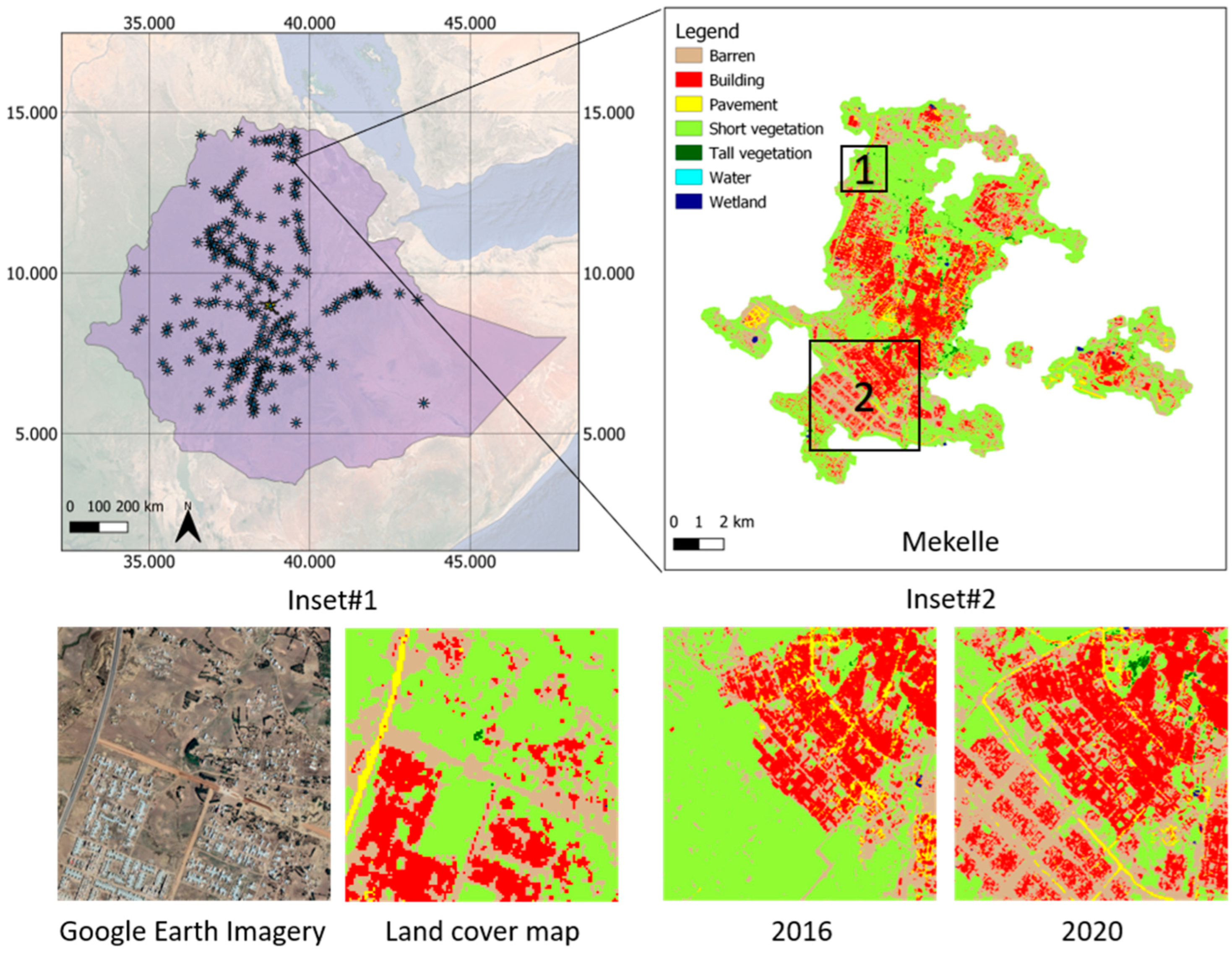
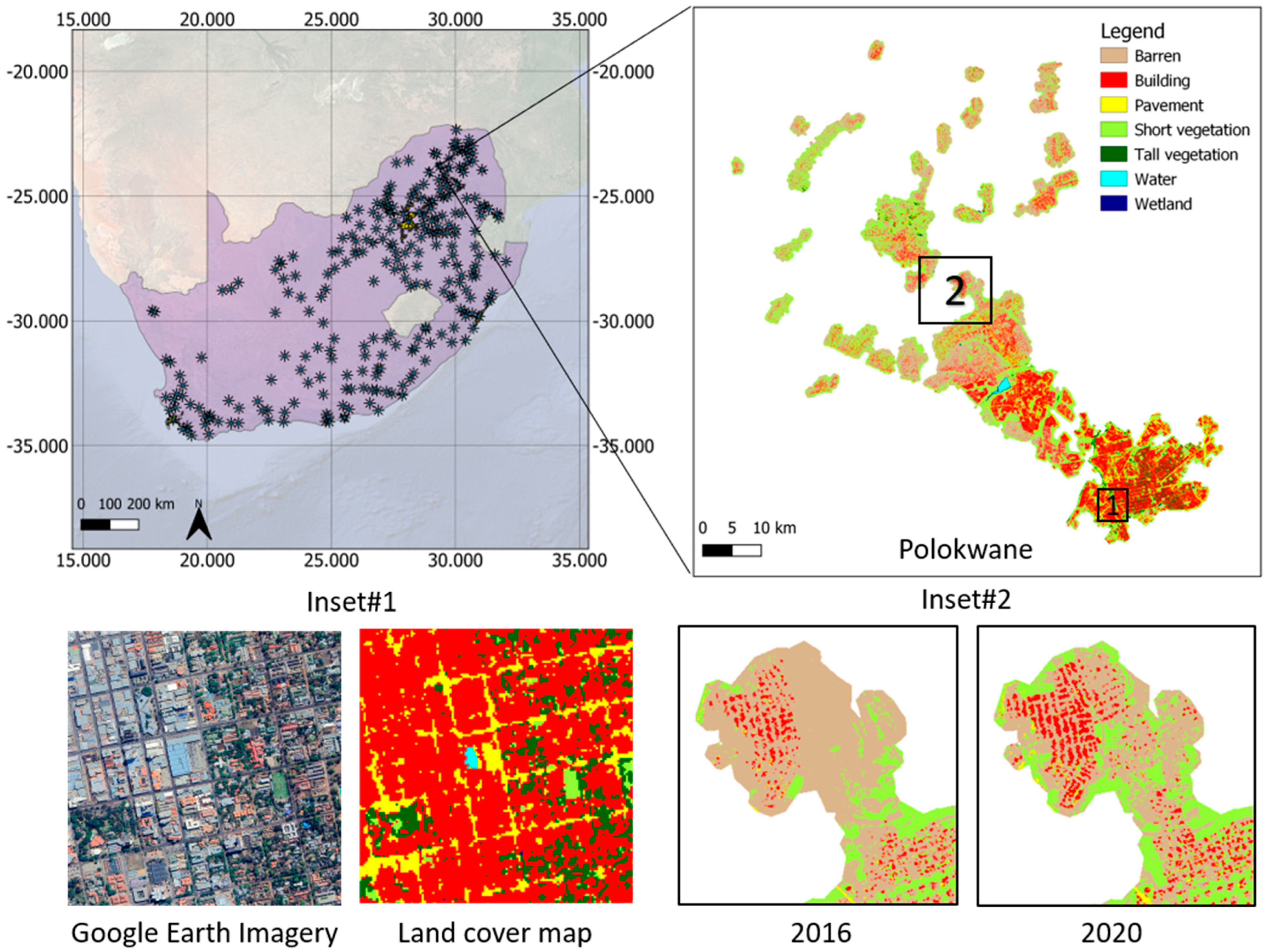
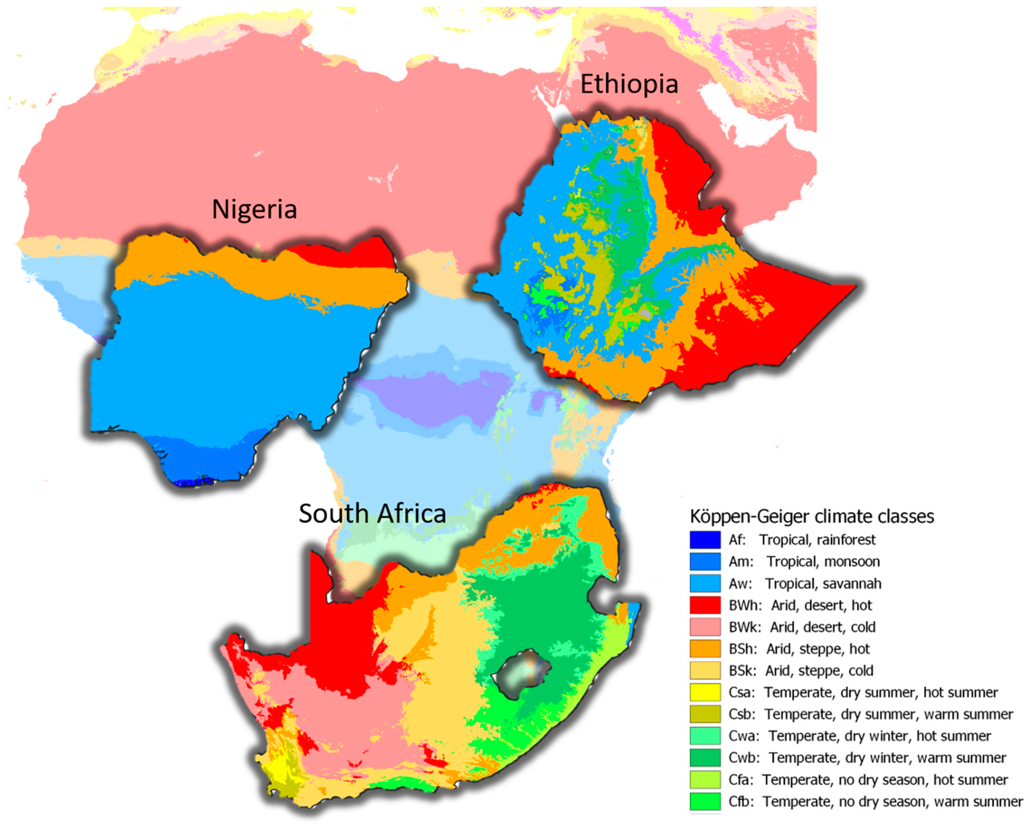
2.1. Study Area
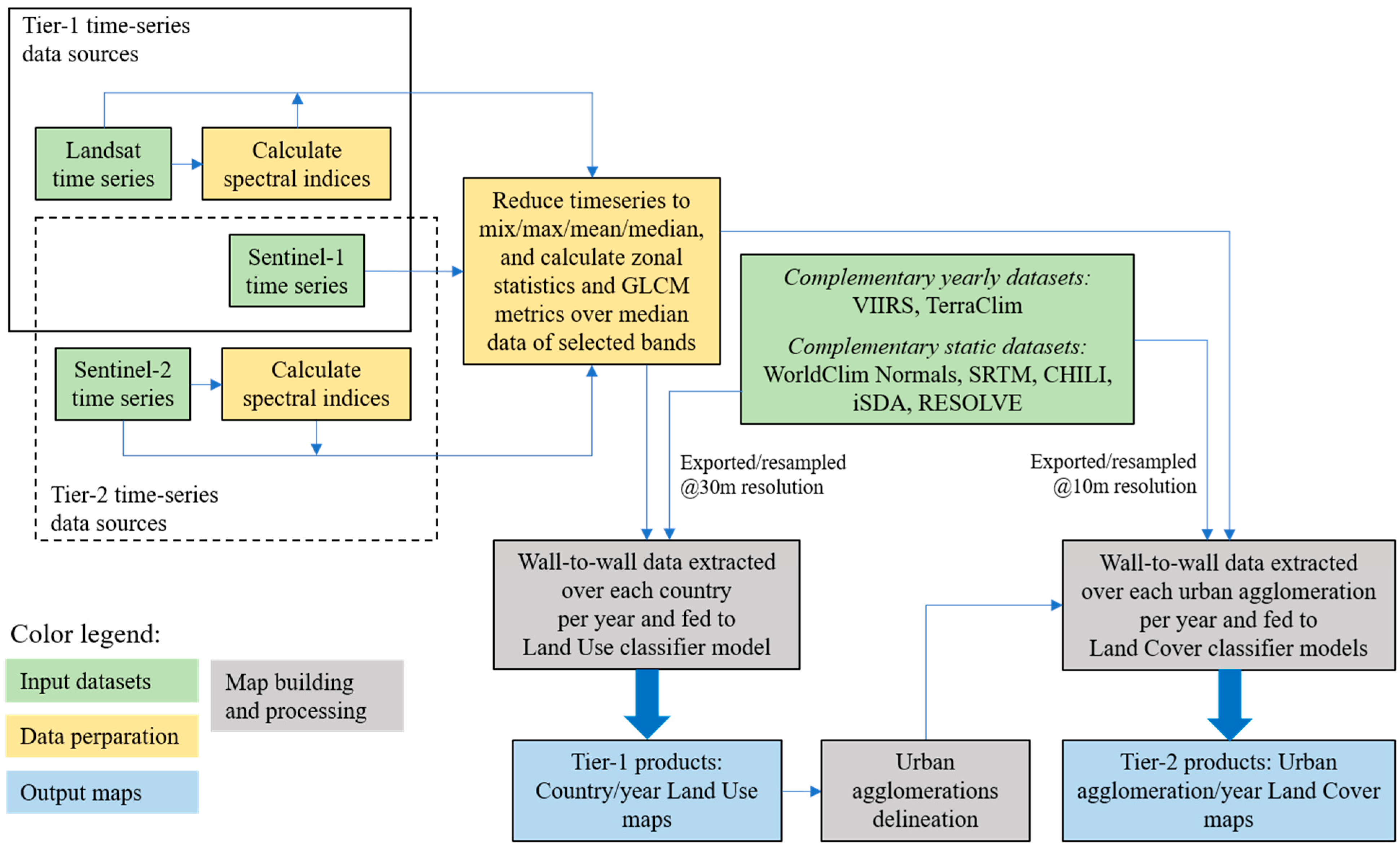
2.2. General Overview
2.3. Remote Sensing Data
2.4. Reference Data Sampling Design and Interpretation
2.5. Model Selection and Map Validation
2.6. Multi-Tiered LULC Analyses
2.6.1. Delineating Urban Boundaries
2.6.2. LU Change Analysis
2.6.3. Characterizing Urban LC Patterns and Change
3. Results
3.1. Tier 1 LU, Tier 2 LC Map Assessments
3.1.1. Tier 1 LU Classification and Change Analyses
3.1.2. LU Distribution and Its Change within Urban Expansion
3.2. Characterizing Urban LC
3.2.1. Annual LC Classification Models and Maps
3.2.2. Urban LC Patterns
4. Discussion
5. Conclusions
Author Contributions
Funding
Data Availability Statement
Acknowledgments
Conflicts of Interest
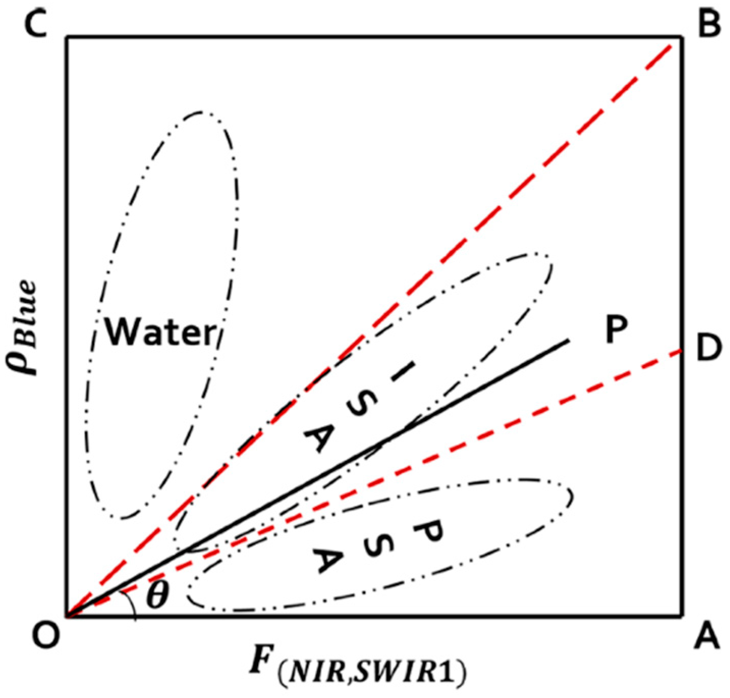
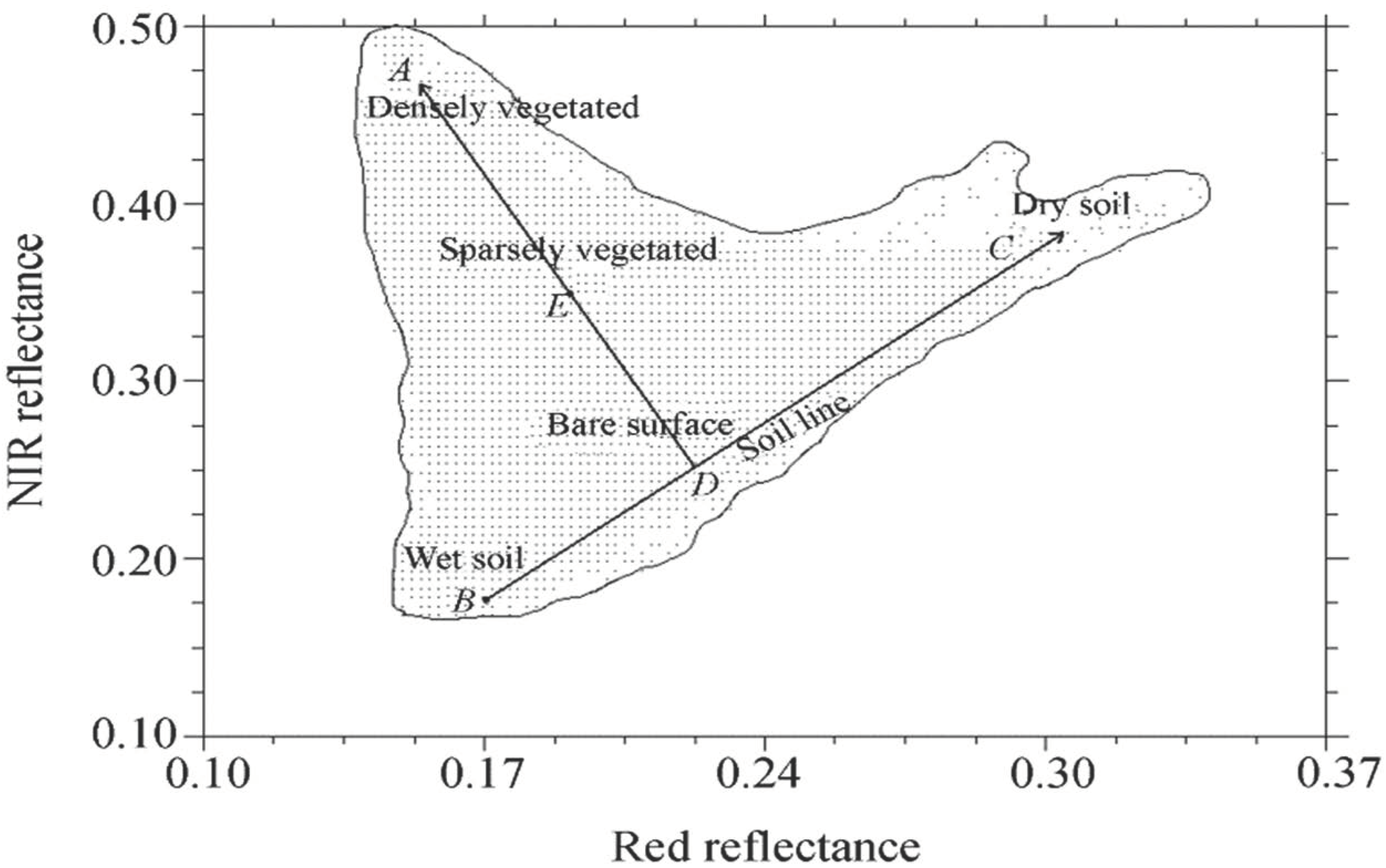
Appendix A. Definition of Spectral Indices and Climate Variables and Their Use in Reference Data Generation

| Landsat Band | ||||||
|---|---|---|---|---|---|---|
| Blue | Green | Red | NIR | SWIR1 | SWIR2 | |
| TCB | 0.2043 | 0.4158 | 0.5524 | 0.5741 | 0.3124 | 0.2303 |
| TCG | −0.1603 | −0.2819 | −0.4934 | 0.794 | −0.0002 | −0.1446 |
| TCW | 0.0315 | 0.2021 | 0.3102 | 0.1594 | −0.6806 | −0.6109 |
| Sentinel-2 Band | ||||||
|---|---|---|---|---|---|---|
| B2 | B2 | B2 | ||||
| TCB | 0.351 | TCB | 0.351 | TCB | 0.351 | TCB |
| TCG | −0.3599 | TCG | −0.3599 | TCG | −0.3599 | TCG |
| TCW | 0.2578 | TCW | 0.2578 | TCW | 0.2578 | TCW |


Appendix B. Land Use and Land Cover Class Definitions
| Land Cover (Tier-1) | Definition |
| Barren | Land composed of bare soil, sand, or rock. Includes dirt and gravel roads. |
| Grass/Herb | Land covered by perennial grasses, forbs, or other forms of herbaceous vegetation. |
| Impervious | Land covered with man-made materials that water cannot penetrate, such as paved roads, rooftops, and parking lots. |
| Shrub | Land vegetated with shrubs. |
| Tree | Land composed of live or standing dead trees. |
| Water | Land covered by water. |
| Land Use (Tier-1) | Definition |
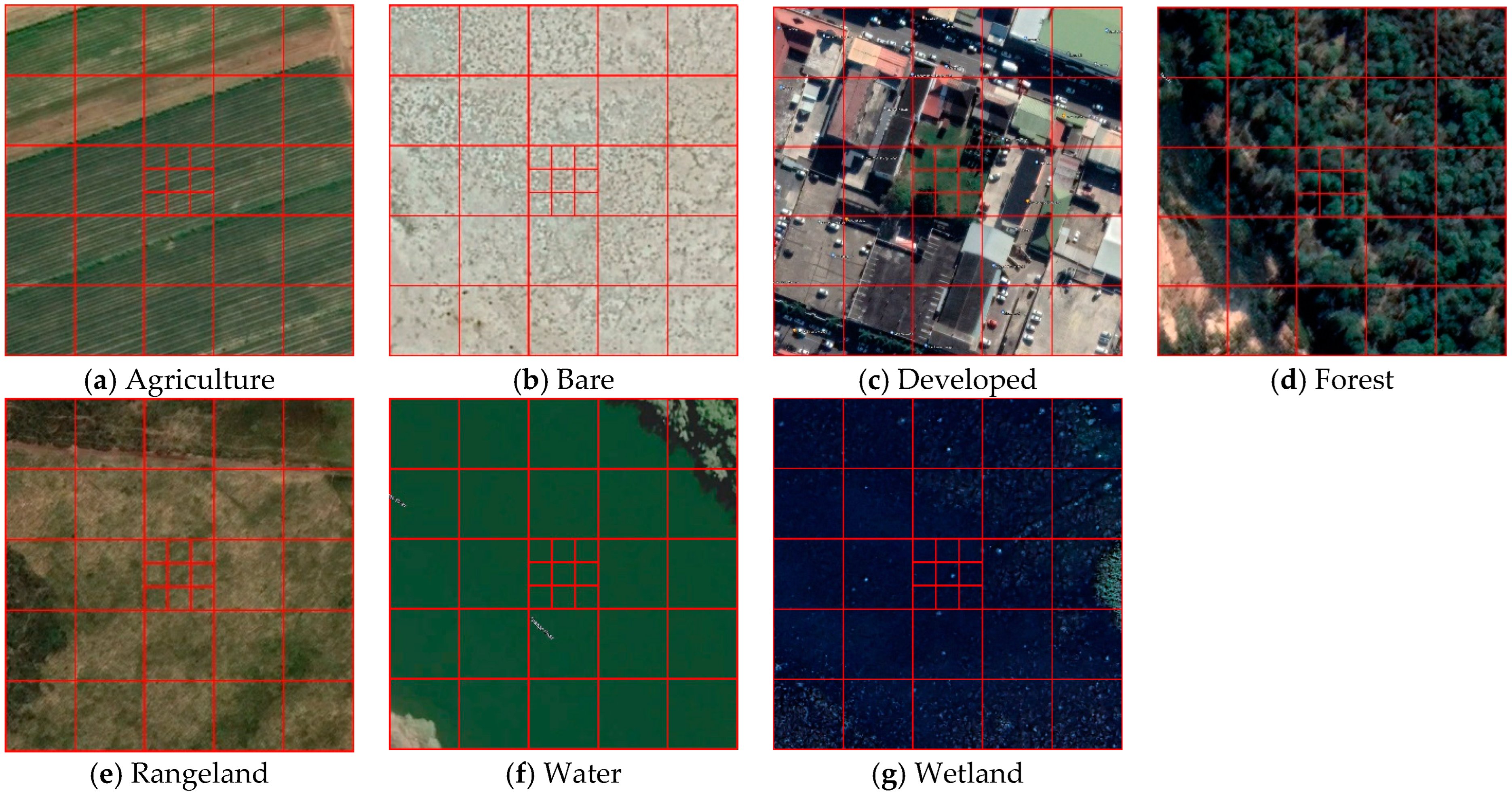
| Agriculture | Land on which the intense agricultural processes are carried (tilling, harvesting, etc.), including orchards and vineyards. Note: roads used primarily for agricultural use (i.e., not used for public transport from town to town) are considered agricultural land use. |
| Bare | Land that lacks the possibility of growing vegetation on more than 80% of the area (20 pixels or more in a 5 × 5 grid). Examples include rocky areas and sandy deserts. Mudflats and sandy deposits at the river banks are also considered bare land if they have no vegetation. |
| Developed | Mostly specified by impervious surfaces but may include other human development on the land such as parks, lawns, cemeteries, mines, and connecting roads (either paved or wide dirt roads that can support two-way traffic with a typical width of at least 20–24 feet). |
| Forest | Closed or open canopy tree stands. At least 20% of the area (5 pixels or more in the 5 × 5 grid) should have trees as their primary land cover. Note: plantations are considered forest land use. |
| Rangeland, which is one of: -Grassland -Open Shrubland -Dense Shrubland -Woodland | Possibly sparse trees with dominant shrubs and/or grass: Woodland: area with existing trees but with less density than qualifies for forest call. We should still have at least 5 pixels in a 5 × 5 grid containing trees but not primary land cover. Shrubland: area with existing shrubs and not qualified as woodland. Shrubland is dense if it contains at least 5 pixels in a 5 × 5 neighborhood containing shrubs as primary land cover. If there are shrubs in at least 5 pixels but it is not primary land cover in all (or any) of them, then it will be open shrubland. Grassland: area with possible herbaceous vegetation growing on most of its surface Note 1: Pasture and grazing lands are considered Grasslands. Note 2: Woodland label has preference over shrubland and shrubland over grassland. If we have enough trees to call the pixel woodland, we do not count the shrub population. If we have enough shrubs to call the pixel shrubland, we do not look at the grass population. |
| Water | Land submerged for more than 80% of the year. |
| Wetland | Land with saturated water level, which can periodically be covered by water (at least 20% of the year). |
| Land Cover (Tier-2) | Definition |
|---|---|
| Barren | Land composed of bare soil, sand, or rock. Includes dirt and gravel roads. |
| Building | Land composed of man-made above-ground structures such as houses, residential and commercial buildings |
| Pavement | Land paved as impervious surface (asphalt, concrete, or stone-paved) |
| Short vegetation | Land covered by perennial grasses, forbs, or other forms of herbaceous and low vegetation. |
| Tall vegetation | Land composed of live or standing dead trees or high shrubs, making a visible shaded area. |
| Water | Land submerged for more than 80% of the year. |
| Wetland | Land with saturated water level, which can periodically be covered by water (at least 20% of the year). |
Appendix C. Reference Data Interpretation

Appendix D. Selected Classification Predictor Features for Each Tier/Country Model
| Ethiopia | Nigeria | South Africa | |||
|---|---|---|---|---|---|
| Feature | Importance | Feature | Importance | Feature | Importance |
| ntl_data | 0.033 | swir2_YearMax | 0.045 | ntl_data | 0.031 |
| tcw_YearMean | 0.032 | VV_YearMean | 0.040 | swir1_YearMean | 0.019 |
| bio_11 | 0.025 | VV_YearMin | 0.037 | UCI_YearMean | 0.015 |
| ndvi_YearMax | 0.024 | swir1_YearMax | 0.033 | VV_YearMin | 0.014 |
| tca_YearMin | 0.019 | soil_data | 0.029 | green_YearMean | 0.013 |
| swir2_YearMin | 0.019 | VV_YearMax | 0.023 | UCI_YearMin | 0.013 |
| bio_16 | 0.017 | ntl_data | 0.022 | swir2_YearMean | 0.013 |
| bio_03 | 0.014 | elevation | 0.015 | VV_max_3 × 3 | 0.011 |
| VV_min_5 × 5 | 0.013 | slope | 0.015 | VV_min_3 × 3 | 0.010 |
| UCI_YearMin | 0.012 | bio_07 | 0.014 | water_perc | 0.009 |
| tcg_min_3 × 3 | 0.012 | bio_08 | 0.014 | bio_08 | 0.009 |
| bio_04 | 0.010 | bio_13 | 0.014 | red_YearMin | 0.009 |
| bio_18 | 0.010 | UCI_YearMax | 0.014 | tcw_max_5 × 5 | 0.009 |
| nir_max_3 × 3 | 0.010 | bio_09 | 0.013 | tcw_max_3 × 3 | 0.009 |
| ndvi_YearRange | 0.009 | nir_YearMax | 0.012 | bio_19 | 0.008 |
| water_perc | 0.009 | red_YearMax | 0.011 | nir_max_3 × 3 | 0.008 |
| slope | 0.009 | bio_18 | 0.010 | nir_YearMax | 0.008 |
| green_max_5 × 5 | 0.008 | water_perc | 0.010 | bio_16 | 0.008 |
| UCI_YearMax | 0.008 | aspect | 0.009 | UCI_YearMax | 0.008 |
| bio_02 | 0.008 | WI_YearMax | 0.007 | nir_min_3 × 3 | 0.007 |
| ECO_ID | 0.008 | max_year_temperature | 0.007 | nir_YearMean | 0.007 |
| tcg_YearRange | 0.008 | blue_YearMax | 0.007 | blue_YearMean | 0.007 |
| VV_asm_5 × 64 | 0.007 | green_YearMax | 0.007 | VV_YearMean | 0.007 |
| soil_data | 0.007 | min_year_temperature | 0.006 | elevation | 0.007 |
| VV_YearRange | 0.007 | CHILI_ind | 0.005 | nir_max_5 × 5 | 0.007 |
| VV_prom_13 × 64 | 0.006 | total_year_rain | 0.005 | red_YearMean | 0.007 |
| tcb_max_3 × 3 | 0.006 | bio_14 | 0.004 | VV_YearMax | 0.006 |
| bio_14 | 0.006 | ECO_ID | 0.004 | nir_min_5 × 5 | 0.006 |
| bio_15 | 0.006 | WI_YearMax | 0.006 | ||
| swir2_YearRange | 0.006 | bio_05 | 0.006 | ||
| UCI_YearRange | 0.005 | slope | 0.006 | ||
| green_YearMin | 0.005 | green_YearMin | 0.005 | ||
| bio_19 | 0.005 | CHILI_ind | 0.005 | ||
| VV_corr_17 × 64 | 0.005 | WI_YearMean | 0.005 | ||
| bio_07 | 0.004 | tcw_min_3 × 3 | 0.005 | ||
| CHILI_ind | 0.004 | swir2_YearMax | 0.005 | ||
| VV_imcorr1_9 × 64 | 0.003 | swir1_YearMin | 0.004 | ||
| WI_YearMin | 0.003 | swir1_YearMax | 0.004 | ||
| green_YearMax | 0.003 | swir2_YearMin | 0.004 | ||
| VV_shade_5 × 64 | 0.003 | blue_YearMin | 0.004 | ||
| VV_shade_9 × 64 | 0.002 | green_YearMax | 0.003 | ||
| VV_shade_13 × 64 | 0.002 | min_year_temperature | 0.003 | ||
| WI_YearMax | 0.002 | blue_YearMax | 0.003 | ||
| WI_YearRange | 0.002 | aspect | 0.003 | ||
| aspect | 0.002 | red_YearMax | 0.003 | ||
| VV_corr_5 × 64 | 0.002 | tcw_min_5 × 5 | 0.003 | ||
| tcb_YearRange | 0.001 | nir_YearMin | 0.002 | ||
| green_YearRange | 0.001 | WI_YearMin | 0.002 | ||
| soil_data | 0.001 | ||||
| Ethiopia | Nigeria | South Africa | |||
|---|---|---|---|---|---|
| Feature | Importance | Feature | Importance | Feature | Importance |
| tca_YearMin | 0.116 | uci_YearMean | 0.086 | VV_YearMean | 0.083 |
| B4_YearMin | 0.109 | ndvi_YearMean | 0.059 | uci_YearMean | 0.078 |
| water_percentage | 0.098 | B11_YearMin | 0.055 | B12_YearMean | 0.072 |
| mndwi_YearMin | 0.064 | VV_YearMean | 0.054 | tcg_YearMean | 0.06 |
| tca_YearRange | 0.058 | tca_YearMax | 0.051 | B12_YearMin | 0.057 |
| VV_min_3 × 3 | 0.051 | mndwi_YearMax | 0.049 | ndvi_YearMin | 0.056 |
| tcb_YearMin | 0.045 | tcg_YearMean | 0.048 | water_percentage | 0.052 |
| B8_stdev_3 × 3 | 0.043 | bai_YearMin | 0.041 | mndwi_YearMax | 0.048 |
| tcb_YearMax | 0.037 | B8_YearMin | 0.035 | tca_YearRange | 0.045 |
| B12_YearRange | 0.035 | water_percentage | 0.034 | B3_YearMin | 0.044 |
| nbai_YearMean | 0.031 | baei_YearMin | 0.029 | tcb_YearMin | 0.033 |
| tcg_stdev_5 × 5 | 0.028 | B2_YearMin | 0.027 | wi_YearMax | 0.023 |
| tcw_stdev_5 × 5 | 0.028 | baei_YearRange | 0.025 | B8_savg_5 × 64 | 0.02 |
| B8_imcorr1_5 × 64 | 0.026 | tcg_stdev_3 × 3 | 0.024 | B2_YearMax | 0.019 |
| B4_YearRange | 0.023 | tcg_YearRange | 0.022 | tcg_stdev_5 × 5 | 0.019 |
| B8_savg_9 × 64 | 0.023 | B8_max_5 × 5 | 0.02 | bai_YearRange | 0.019 |
| VV_asm_9 × 64 | 0.022 | uci_YearRange | 0.019 | B3_stdev_3 × 3 | 0.018 |
| B8_contrast_9 × 64 | 0.02 | VV_savg_9 × 64 | 0.019 | nbai_YearMin | 0.017 |
| B8_shade_9 × 64 | 0.015 | mndwi_YearRange | 0.019 | B8_stdev_5 × 5 | 0.014 |
| nbai_YearRange | 0.014 | B12_YearRange | 0.017 | B8_imcorr1_9 × 64 | 0.014 |
| VV_YearRange | 0.011 | bio_03 | 0.016 | B8_YearRange | 0.013 |
| VV_shade_5 × 64 | 0.01 | B8_stdev_3 × 3 | 0.015 | tcw_YearRange | 0.012 |
| VV_corr_5 × 64 | 0.01 | elevation | 0.013 | B3_YearRange | 0.011 |
| VV_corr_9 × 64 | 0.01 | nbai_YearMean | 0.012 | nbai_YearMax | 0.01 |
| ntl_data | 0.009 | tcb_YearRange | 0.011 | nbai_YearRange | 0.01 |
| bio_16 | 0.007 | bio_13 | 0.011 | ntl_data | 0.009 |
| bio_15 | 0.007 | VV_imcorr1_9 × 64 | 0.011 | tcw_stdev_3 × 3 | 0.009 |
| bio_10 | 0.007 | B8_shade_9 × 64 | 0.01 | B8_contrast_9 × 64 | 0.008 |
| bio_03 | 0.007 | B3_stdev_5 × 5 | 0.01 | B8_corr_5 × 64 | 0.008 |
| bio_12 | 0.007 | B3_min_5 × 5 | 0.01 | VV_stdev_5 × 5 | 0.008 |
| bio_02 | 0.007 | min_year_temperature | 0.009 | B8_shade_5 × 64 | 0.008 |
| bio_14 | 0.006 | bio_10 | 0.009 | B8_shade_9 × 64 | 0.008 |
| aspect | 0.005 | nbai_YearMax | 0.009 | VV_shade_9 × 64 | 0.007 |
| slope | 0.005 | B8_imcorr2_9 × 64 | 0.009 | bio_10 | 0.006 |
| soil_data | 0.004 | VV_asm_5 × 64 | 0.008 | VV_prom_5 × 64 | 0.006 |
| ECO_ID | 0.002 | tcb_stdev_5 × 5 | 0.008 | VV_shade_5 × 64 | 0.006 |
| B8_shade_5 × 64 | 0.007 | B8_imcorr2_5 × 64 | 0.006 | ||
| B8_prom_9 × 64 | 0.007 | bio_15 | 0.006 | ||
| VV_contrast_5 × 64 | 0.007 | VV_corr_5 × 64 | 0.006 | ||
| VV_stdev_5 × 5 | 0.006 | VV_imcorr2_9 × 64 | 0.006 | ||
| B8_contrast_9 × 64 | 0.006 | bio_04 | 0.005 | ||
| B8_corr_5 × 64 | 0.006 | bio_17 | 0.005 | ||
| tcw_stdev_3 × 3 | 0.006 | bio_06 | 0.005 | ||
| B2_YearRange | 0.006 | bio_05 | 0.005 | ||
| VV_shade_5 × 64 | 0.006 | bio_03 | 0.005 | ||
| VV_shade_9 × 64 | 0.006 | aspect | 0.004 | ||
| bio_01 | 0.005 | VV_YearRange | 0.004 | ||
| VV_YearRange | 0.005 | slope | 0.004 | ||
| aspect | 0.005 | total_year_rain | 0.004 | ||
| VV_imcorr2_5 × 64 | 0.005 | ECO_ID | 0.003 | ||
| ntl_data | 0.005 | soil_data | 0.001 | ||
| ECO_ID | 0.004 | ||||
| slope | 0.003 | ||||
| soil_data | 0.001 | ||||
Appendix D.1. Addressing Blocky Artifacts in Tier-1 Products
Appendix E. Classification Confusion Matrix and Map Accuracy Assessment Tables for Target Countries and Study Years
| Country | Agriculture | Bare | Developed | Forest | Rangeland | Water | Wetland |
|---|---|---|---|---|---|---|---|
| Ethiopia | 22.5% | 5.8% | 0.8% | 13.5% | 55.6% | 0.7% | 1.1% |
| Nigeria | 47.4% | 0.2% | 2.6% | 16.4% | 31.3% | 0.5% | 1.5% |
| South Africa | 9.2% | 3.3% | 1.8% | 6.0% | 79.2% | 0.4% | 0.0% |
| Country | Barren | Building | Pavement | Short Vegetation | Tall Vegetation | Water | Wetland |
|---|---|---|---|---|---|---|---|
| Ethiopia | 14.0% | 5.2% | 1.9% | 64.8% | 12.5% | 0.9% | 0.6% |
| Nigeria | 2.0% | 29.9% | 22.7% | 18.5% | 25.6% | 0.6% | 0.6% |
| South Africa | 8.2% | 29.5% | 13.5% | 35.4% | 12.0% | 0.2% | 1.2% |
| Year 2020 | |||||||||||
|---|---|---|---|---|---|---|---|---|---|---|---|
| Ethiopia: | |||||||||||
| Reference | |||||||||||
| Predicted | Agriculture | Bare | Developed | Forest | Range | Water | Wetland | Precision (UA) | F1 | Map UA | 95% CI |
| Agriculture | 51 | 0 | 7 | 2 | 17 | 0 | 1 | 65.38 | 65.81 | 61.22 | 14.95 |
| Bare | 0 | 50 | 0 | 0 | 22 | 0 | 0 | 69.44 | 79.37 | 45.52 | 20.31 |
| Developed | 6 | 0 | 41 | 1 | 17 | 0 | 0 | 63.08 | 70.69 | 33.14 | 32.67 |
| Forest | 2 | 0 | 2 | 50 | 17 | 0 | 4 | 66.67 | 72.99 | 76.42 | 10.93 |
| Range | 16 | 4 | 1 | 8 | 103 | 0 | 11 | 72.03 | 60.59 | 86.35 | 8.50 |
| Water | 0 | 0 | 0 | 0 | 0 | 58 | 2 | 96.67 | 98.31 | 96.66 | 4.69 |
| Wetland | 2 | 0 | 0 | 1 | 21 | 0 | 33 | 57.89 | 61.11 | 57.71 | 13.17 |
| Recall (PA) | 66.23 | 92.59 | 80.39 | 80.65 | 52.28 | 100.00 | 64.71 | 70.18 | 72.69 | ||
| OA | AvgF1 | ||||||||||
| Map PA | 76.96 | 95.77 | 23.41 | 80.23 | 71.95 | 100.00 | 64.69 | Map OA | 95% CI | ||
| 95% CI | 14.34 | 5.39 | 21.00 | 18.82 | 10.17 | 0.00 | 13.51 | 74.62 | 7.26 | ||
| % of Map OA | 24% | 6% | 1% | 14% | 55% | 1% | 1% | ||||
| Nigeria: | |||||||||||
| Reference | |||||||||||
| Predicted | Agriculture | Bare | Developed | Forest | Range | Water | Wetland | Precision (UA) | F1 | Map UA | 95% CI |
| Agriculture | 77 | 4 | 16 | 8 | 42 | 0 | 5 | 50.66 | 60.16 | 72.38 | 8.21 |
| Bare | 0 | 17 | 0 | 0 | 4 | 0 | 0 | 80.95 | 47.22 | 80.95 | 17.96 |
| Developed | 0 | 0 | 45 | 1 | 4 | 0 | 0 | 90.00 | 73.77 | 81.51 | 19.79 |
| Forest | 2 | 0 | 3 | 56 | 29 | 0 | 12 | 54.90 | 58.33 | 62.69 | 11.17 |
| Range | 24 | 30 | 8 | 25 | 112 | 0 | 9 | 53.85 | 54.50 | 57.90 | 9.11 |
| Water | 0 | 0 | 0 | 0 | 0 | 85 | 16 | 84.16 | 89.95 | 75.30 | 10.72 |
| Wetland | 1 | 0 | 0 | 0 | 12 | 3 | 50 | 75.76 | 63.29 | 78.28 | 11.62 |
| Recall (PA) | 74.04 | 33.33 | 62.50 | 62.22 | 55.17 | 96.59 | 54.35 | 63.14 | 63.89 | ||
| OA | AvgF1 | ||||||||||
| Map PA | 77.41 | 27.88 | 47.79 | 58.96 | 57.38 | 92.94 | 49.74 | Map OA | 95% CI | ||
| 95% CI | 8.24 | 15.02 | 21.09 | 11.27 | 8.99 | 8.14 | 22.27 | 65.85 | 5.44 | ||
| % of Map OA | 50% | 0% | 2% | 14% | 31% | 1% | 1% | ||||
| South Africa | |||||||||||
| Reference | |||||||||||
| Predicted | Agriculture | Bare | Developed | Forest | Range | Water | Wetland | Precision (UA) | F1 | Map UA | 95% CI |
| Agriculture | 86 | 0 | 21 | 4 | 30 | 2 | 2 | 59.31 | 71.07 | 64.71 | 18.44 |
| Bare | 0 | 59 | 3 | 3 | 9 | 2 | 6 | 71.95 | 44.87 | 53.69 | 42.79 |
| Developed | 0 | 2 | 69 | 0 | 4 | 0 | 0 | 92.00 | 64.19 | 92.00 | 6.26 |
| Forest | 0 | 2 | 1 | 88 | 63 | 4 | 13 | 51.46 | 62.41 | 53.65 | 18.49 |
| Range | 11 | 116 | 41 | 4 | 141 | 2 | 3 | 44.34 | 47.39 | 77.42 | 7.72 |
| Water | 0 | 1 | 3 | 10 | 13 | 112 | 35 | 64.37 | 75.68 | 86.32 | 6.00 |
| Wetland | 0 | 1 | 2 | 2 | 17 | 0 | 11 | 33.33 | 21.36 | 67.62 | 35.86 |
| Recall (PA) | 88.66 | 32.60 | 49.29 | 79.28 | 50.90 | 91.80 | 15.71 | 56.71 | 55.28 | ||
| OA | AvgF1 | ||||||||||
| Map PA | 89.92 | 6.85 | 24.11 | 82.91 | 88.51 | 98.79 | 8.28 | Map OA | 95% CI | ||
| 95% CI | 6.28 | 2.92 | 18.57 | 22.76 | 5.55 | 1.90 | 12.39 | 73.60 | 6.82 | ||
| % of Map OA | 10% | 2% | 1% | 6% | 81% | 0% | 0% | ||||
| Year 2019 | |||||||||||
|---|---|---|---|---|---|---|---|---|---|---|---|
| Ethiopia: | |||||||||||
| Reference | |||||||||||
| Predicted | Agriculture | Bare | Developed | Forest | Range | Water | Wetland | Precision (UA) | F1 | Map UA | 95% CI |
| Agriculture | 53 | 0 | 8 | 1 | 13 | 0 | 2 | 68.83 | 68.83 | 70.10 | 15.16 |
| Bare | 0 | 50 | 0 | 0 | 22 | 0 | 0 | 69.44 | 79.37 | 45.52 | 20.31 |
| Developed | 4 | 0 | 40 | 1 | 12 | 0 | 0 | 70.18 | 74.07 | 17.93 | 27.20 |
| Forest | 2 | 0 | 2 | 52 | 16 | 0 | 4 | 68.42 | 75.36 | 73.50 | 14.42 |
| Range | 17 | 3 | 1 | 7 | 121 | 0 | 11 | 75.63 | 67.41 | 88.31 | 7.55 |
| Water | 0 | 0 | 0 | 0 | 0 | 57 | 2 | 96.61 | 98.28 | 96.61 | 4.76 |
| Wetland | 1 | 1 | 0 | 1 | 15 | 0 | 31 | 63.27 | 62.63 | 63.03 | 13.94 |
| Recall (PA) | 68.83 | 92.59 | 78.43 | 83.87 | 60.80 | 100.00 | 62.00 | 73.45 | 75.13 | ||
| OA | AvgF1 | ||||||||||
| Map PA | 80.32 | 95.77 | 22.84 | 81.90 | 74.84 | 100.00 | 61.99 | Map OA | 95% CI | ||
| 95% CI | 12.72 | 5.39 | 20.52 | 18.91 | 9.78 | 0.00 | 13.86 | 77.25 | 6.93 | ||
| % of Map OA | 23% | 5% | 1% | 14% | 56% | 1% | 1% | ||||
| Nigeria: | |||||||||||
| Reference | |||||||||||
| Predicted | Agriculture | Bare | Developed | Forest | Range | Water | Wetland | Precision (UA) | F1 | Map UA | 95% CI |
| Agriculture | 78 | 4 | 17 | 5 | 52 | 0 | 4 | 48.75 | 59.54 | 69.55 | 8.35 |
| Bare | 0 | 15 | 0 | 0 | 4 | 0 | 0 | 78.95 | 43.48 | 78.95 | 19.74 |
| Developed | 0 | 0 | 45 | 3 | 3 | 0 | 0 | 88.24 | 73.17 | 80.06 | 19.40 |
| Forest | 2 | 0 | 1 | 65 | 31 | 0 | 14 | 57.52 | 63.73 | 63.53 | 10.43 |
| Range | 21 | 31 | 9 | 18 | 100 | 0 | 10 | 52.91 | 50.76 | 59.99 | 9.81 |
| Water | 0 | 0 | 0 | 0 | 0 | 85 | 13 | 86.73 | 91.40 | 80.91 | 10.06 |
| Wetland | 1 | 0 | 0 | 0 | 15 | 3 | 51 | 72.86 | 62.96 | 59.91 | 28.66 |
| Recall (PA) | 76.47 | 30.00 | 62.50 | 71.43 | 48.78 | 96.59 | 55.43 | 62.71 | 63.58 | ||
| OA | AvgF1 | ||||||||||
| Map PA | 79.59 | 25.01 | 47.79 | 69.98 | 49.93 | 92.79 | 50.92 | Map OA | 95% CI | ||
| 95% CI | 7.99 | 14.27 | 21.09 | 10.57 | 8.88 | 8.27 | 22.40 | 65.55 | 5.46 | ||
| % of Map OA | 51% | 0% | 2% | 15% | 30% | 1% | 1% | ||||
| South Africa | |||||||||||
| Reference | |||||||||||
| Predicted | Agriculture | Bare | Developed | Forest | Range | Water | Wetland | Precision (UA) | F1 | Map UA | 95% CI |
| Agriculture | 83 | 0 | 24 | 4 | 29 | 1 | 3 | 57.64 | 69.46 | 68.59 | 17.81 |
| Bare | 0 | 59 | 4 | 3 | 12 | 2 | 5 | 69.41 | 45.04 | 93.21 | 6.67 |
| Developed | 0 | 2 | 64 | 0 | 4 | 0 | 0 | 91.43 | 60.95 | 91.43 | 6.69 |
| Forest | 0 | 3 | 2 | 88 | 59 | 1 | 16 | 52.07 | 62.63 | 54.20 | 18.79 |
| Range | 12 | 113 | 40 | 6 | 149 | 1 | 6 | 45.57 | 48.93 | 78.49 | 7.53 |
| Water | 0 | 0 | 3 | 9 | 12 | 111 | 35 | 65.29 | 77.62 | 85.10 | 6.20 |
| Wetland | 0 | 0 | 3 | 2 | 17 | 0 | 12 | 35.29 | 21.62 | 37.50 | 17.43 |
| Recall (PA) | 87.37 | 33.33 | 45.71 | 78.57 | 52.84 | 95.69 | 15.58 | 56.66 | 55.18 | ||
| OA | AvgF1 | ||||||||||
| Map PA | 88.70 | 16.83 | 22.36 | 82.07 | 89.78 | 99.86 | 2.23 | Map OA | 95% CI | ||
| 95% CI | 6.74 | 13.52 | 17.29 | 22.46 | 5.11 | 0.12 | 1.58 | 75.89 | 6.53 | ||
| % of Map OA | 9% | 2% | 1% | 6% | 81% | 0% | 0% | ||||
| Year 2018 | |||||||||||
|---|---|---|---|---|---|---|---|---|---|---|---|
| Ethiopia: | |||||||||||
| Reference | |||||||||||
| Predicted | Agriculture | Bare | Developed | Forest | Range | Water | Wetland | Precision (UA) | F1 | Map UA | 95% CI |
| Agriculture | 60 | 0 | 9 | 3 | 16 | 0 | 2 | 66.67 | 71.01 | 73.54 | 13.86 |
| Bare | 0 | 51 | 0 | 0 | 22 | 0 | 0 | 69.86 | 80.31 | 46.01 | 20.31 |
| Developed | 2 | 0 | 36 | 0 | 12 | 0 | 0 | 72.00 | 74.23 | 9.42 | 11.85 |
| Forest | 3 | 0 | 1 | 49 | 10 | 0 | 2 | 75.38 | 76.56 | 75.58 | 15.00 |
| Range | 13 | 3 | 1 | 9 | 125 | 0 | 15 | 75.30 | 67.39 | 89.07 | 7.64 |
| Water | 0 | 0 | 0 | 0 | 0 | 57 | 1 | 98.28 | 98.28 | 98.28 | 3.45 |
| Wetland | 1 | 0 | 0 | 2 | 20 | 1 | 24 | 50.00 | 52.17 | 50.00 | 14.59 |
| Recall (PA) | 75.95 | 94.44 | 76.60 | 77.78 | 60.98 | 98.28 | 54.55 | 73.09 | 74.28 | ||
| OA | AvgF1 | ||||||||||
| Map PA | 84.92 | 97.69 | 21.04 | 80.09 | 74.12 | 98.53 | 54.94 | Map OA | 95% CI | ||
| 95% CI | 11.61 | 3.87 | 19.46 | 18.78 | 9.94 | 2.89 | 15.22 | 77.66 | 6.91 | ||
| % of Map OA | 23% | 5% | 1% | 14% | 55% | 1% | 1% | ||||
| Nigeria: | |||||||||||
| Reference | |||||||||||
| Predicted | Agriculture | Bare | Developed | Forest | Range | Water | Wetland | Precision (UA) | F1 | Map UA | 95% CI |
| Agriculture | 73 | 3 | 22 | 10 | 45 | 0 | 5 | 46.20 | 56.81 | 68.14 | 8.55 |
| Bare | 0 | 17 | 0 | 0 | 4 | 0 | 0 | 80.95 | 47.89 | 80.95 | 17.96 |
| Developed | 0 | 0 | 42 | 3 | 4 | 0 | 0 | 85.71 | 69.42 | 77.48 | 19.86 |
| Forest | 3 | 0 | 1 | 63 | 30 | 0 | 15 | 56.25 | 62.07 | 61.15 | 10.57 |
| Range | 22 | 30 | 7 | 15 | 112 | 0 | 11 | 56.85 | 55.58 | 62.95 | 9.44 |
| Water | 0 | 0 | 0 | 0 | 0 | 83 | 16 | 83.84 | 90.22 | 79.70 | 9.72 |
| Wetland | 1 | 0 | 0 | 0 | 11 | 2 | 50 | 78.13 | 62.11 | 81.09 | 10.79 |
| Recall (PA) | 73.74 | 34.00 | 58.33 | 69.23 | 54.37 | 97.65 | 51.55 | 62.86 | 63.44 | ||
| OA | AvgF1 | ||||||||||
| Map PA | 77.44 | 28.34 | 44.60 | 65.55 | 54.92 | 95.64 | 49.56 | Map OA | 95% CI | ||
| 95% CI | 8.41 | 15.35 | 20.01 | 11.13 | 8.77 | 6.57 | 21.44 | 65.50 | 5.47 | ||
| % of Map OA | 50% | 0% | 2% | 14% | 32% | 1% | 1% | ||||
| South Africa | |||||||||||
| Reference | |||||||||||
| Predicted | Agriculture | Bare | Developed | Forest | Range | Water | Wetland | Precision (UA) | F1 | Map UA | 95% CI |
| Agriculture | 82 | 1 | 24 | 3 | 28 | 2 | 4 | 56.94 | 69.20 | 74.88 | 15.73 |
| Bare | 2 | 55 | 4 | 3 | 10 | 2 | 6 | 67.07 | 41.98 | 89.47 | 11.00 |
| Developed | 0 | 1 | 59 | 0 | 5 | 1 | 0 | 89.39 | 57.56 | 90.48 | 7.13 |
| Forest | 0 | 4 | 1 | 90 | 59 | 2 | 12 | 53.57 | 64.52 | 50.53 | 18.44 |
| Range | 9 | 118 | 46 | 6 | 154 | 1 | 7 | 45.16 | 49.12 | 78.63 | 7.52 |
| Water | 0 | 0 | 3 | 5 | 11 | 104 | 31 | 67.53 | 77.04 | 85.47 | 6.30 |
| Wetland | 0 | 1 | 2 | 4 | 19 | 4 | 13 | 30.23 | 22.41 | 55.99 | 41.11 |
| Recall (PA) | 88.17 | 30.56 | 42.45 | 81.08 | 53.85 | 89.66 | 17.81 | 55.81 | 54.55 | ||
| OA | AvgF1 | ||||||||||
| Map PA | 89.50 | 16.39 | 21.04 | 83.08 | 89.86 | 97.76 | 13.15 | Map OA | 95% CI | ||
| 95% CI | 6.56 | 13.49 | 16.44 | 22.57 | 5.10 | 2.73 | 15.01 | 75.95 | 6.53 | ||
| % of Map OA | 9% | 2% | 1% | 6% | 81% | 0% | 0% | ||||
| Year 2017 | |||||||||||
|---|---|---|---|---|---|---|---|---|---|---|---|
| Ethiopia: | |||||||||||
| Reference | |||||||||||
| Predicted | Agriculture | Bare | Developed | Forest | Range | Water | Wetland | Precision (UA) | F1 | Map UA | 95% CI |
| Agriculture | 62 | 0 | 11 | 2 | 19 | 0 | 3 | 63.92 | 70.06 | 69.93 | 14.10 |
| Bare | 0 | 49 | 0 | 0 | 21 | 0 | 0 | 70.00 | 79.67 | 59.31 | 21.55 |
| Developed | 1 | 0 | 33 | 0 | 10 | 0 | 0 | 75.00 | 72.53 | 8.77 | 11.27 |
| Forest | 2 | 0 | 0 | 51 | 7 | 0 | 2 | 82.26 | 82.26 | 87.09 | 9.41 |
| Range | 12 | 4 | 3 | 7 | 135 | 0 | 18 | 75.42 | 69.95 | 90.90 | 6.37 |
| Water | 0 | 0 | 0 | 0 | 0 | 56 | 1 | 98.25 | 98.25 | 98.25 | 3.51 |
| Wetland | 3 | 0 | 0 | 2 | 15 | 1 | 20 | 48.78 | 47.06 | 49.01 | 15.86 |
| Recall (PA) | 77.50 | 92.45 | 70.21 | 82.26 | 65.22 | 98.25 | 45.45 | 73.82 | 74.25 | ||
| OA | AvgF1 | ||||||||||
| Map PA | 84.93 | 95.69 | 19.29 | 88.06 | 78.09 | 98.51 | 46.07 | Map OA | 95% CI | ||
| 95% CI | 11.60 | 5.50 | 17.95 | 15.34 | 9.07 | 2.95 | 15.27 | 80.89 | 6.31 | ||
| % of Map OA | 22% | 5% | 1% | 13% | 57% | 1% | 1% | ||||
| Nigeria: | |||||||||||
| Reference | |||||||||||
| Predicted | Agriculture | Bare | Developed | Forest | Range | Water | Wetland | Precision (UA) | F1 | Map UA | 95% CI |
| Agriculture | 78 | 4 | 25 | 5 | 54 | 0 | 2 | 46.43 | 58.87 | 70.22 | 8.19 |
| Bare | 0 | 18 | 0 | 0 | 4 | 0 | 0 | 81.82 | 50.00 | 81.82 | 17.18 |
| Developed | 0 | 0 | 38 | 2 | 3 | 0 | 0 | 88.37 | 66.09 | 71.14 | 24.64 |
| Forest | 2 | 0 | 2 | 62 | 28 | 0 | 19 | 54.87 | 60.19 | 64.48 | 10.44 |
| Range | 17 | 27 | 7 | 24 | 111 | 0 | 14 | 55.50 | 53.88 | 62.76 | 9.35 |
| Water | 0 | 1 | 0 | 0 | 0 | 83 | 16 | 83.00 | 89.25 | 79.71 | 9.60 |
| Wetland | 0 | 0 | 0 | 0 | 12 | 3 | 39 | 72.22 | 54.17 | 76.07 | 13.75 |
| Recall (PA) | 80.41 | 36.00 | 52.78 | 66.67 | 52.36 | 96.51 | 43.33 | 61.29 | 61.78 | ||
| OA | AvgF1 | ||||||||||
| Map PA | 83.06 | 30.01 | 40.36 | 61.57 | 55.30 | 92.78 | 42.27 | Map OA | 95% CI | ||
| 95% CI | 7.52 | 15.88 | 18.55 | 11.43 | 8.92 | 8.31 | 21.36 | 66.85 | 5.35 | ||
| % of Map OA | 52% | 0% | 2% | 14% | 30% | 1% | 1% | ||||
| South Africa | |||||||||||
| Reference | |||||||||||
| Predicted | Agriculture | Bare | Developed | Forest | Range | Water | Wetland | Precision (UA) | F1 | Map UA | 95% CI |
| Agriculture | 74 | 1 | 18 | 4 | 25 | 2 | 4 | 57.81 | 66.97 | 67.79 | 18.97 |
| Bare | 1 | 50 | 4 | 3 | 12 | 2 | 8 | 62.50 | 39.06 | 90.98 | 9.19 |
| Developed | 0 | 1 | 63 | 1 | 5 | 1 | 0 | 88.73 | 60.00 | 89.74 | 7.11 |
| Forest | 2 | 5 | 2 | 87 | 59 | 2 | 8 | 52.73 | 63.74 | 50.08 | 18.86 |
| Range | 16 | 117 | 47 | 6 | 172 | 7 | 8 | 46.11 | 51.27 | 80.01 | 7.21 |
| Water | 0 | 2 | 3 | 3 | 13 | 98 | 30 | 65.77 | 75.10 | 82.50 | 6.92 |
| Wetland | 0 | 0 | 2 | 4 | 12 | 0 | 13 | 41.94 | 25.49 | 81.39 | 20.04 |
| Recall (PA) | 79.57 | 28.41 | 45.32 | 80.56 | 57.72 | 87.50 | 18.31 | 55.87 | 54.52 | ||
| OA | AvgF1 | ||||||||||
| Map PA | 83.74 | 20.85 | 22.44 | 82.10 | 90.21 | 95.63 | 11.32 | Map OA | 95% CI | ||
| 95% CI | 8.13 | 15.95 | 17.47 | 22.95 | 5.06 | 3.97 | 13.08 | 76.55 | 6.42 | ||
| % of Map OA | 9% | 2% | 1% | 6% | 82% | 0% | 0% | ||||
| Year 2016 | |||||||||||
|---|---|---|---|---|---|---|---|---|---|---|---|
| Ethiopia: | |||||||||||
| Reference | |||||||||||
| Predicted | Agriculture | Bare | Developed | Forest | Range | Water | Wetland | Precision (UA) | F1 | Map UA | 95% CI |
| Agriculture | 65 | 0 | 13 | 4 | 31 | 0 | 2 | 56.52 | 65.33 | 59.95 | 14.38 |
| Bare | 0 | 49 | 0 | 0 | 21 | 0 | 0 | 70.00 | 79.67 | 51.45 | 22.01 |
| Developed | 0 | 0 | 29 | 0 | 7 | 0 | 0 | 80.56 | 71.60 | 14.35 | 24.44 |
| Forest | 2 | 0 | 2 | 51 | 6 | 0 | 2 | 80.95 | 80.95 | 87.23 | 9.26 |
| Range | 14 | 4 | 1 | 7 | 127 | 0 | 15 | 75.60 | 67.73 | 88.63 | 7.01 |
| Water | 0 | 0 | 0 | 0 | 0 | 55 | 1 | 98.21 | 97.35 | 98.21 | 3.58 |
| Wetland | 3 | 0 | 0 | 1 | 15 | 2 | 21 | 50.00 | 50.60 | 50.42 | 15.65 |
| Recall (PA) | 77.38 | 92.45 | 64.44 | 80.95 | 61.35 | 96.49 | 51.22 | 72.18 | 73.32 | ||
| OA | AvgF1 | ||||||||||
| Map PA | 79.76 | 95.69 | 17.15 | 88.21 | 72.51 | 97.01 | 52.06 | Map OA | 95% CI | ||
| 95% CI | 12.53 | 5.50 | 16.30 | 15.10 | 10.29 | 4.10 | 15.86 | 76.51 | 6.98 | ||
| % of Map OA | 22% | 5% | 1% | 14% | 56% | 1% | 1% | ||||
| Nigeria: | |||||||||||
| Reference | |||||||||||
| Predicted | Agriculture | Bare | Developed | Forest | Range | Water | Wetland | Precision (UA) | F1 | Map UA | 95% CI |
| Agriculture | 69 | 4 | 25 | 9 | 48 | 0 | 4 | 43.40 | 54.33 | 67.81 | 8.69 |
| Bare | 0 | 17 | 0 | 0 | 4 | 0 | 0 | 80.95 | 47.89 | 80.95 | 17.96 |
| Developed | 0 | 0 | 38 | 3 | 5 | 0 | 0 | 82.61 | 64.96 | 61.67 | 22.95 |
| Forest | 3 | 0 | 1 | 66 | 26 | 0 | 17 | 58.41 | 62.56 | 65.33 | 10.85 |
| Range | 23 | 28 | 7 | 20 | 115 | 1 | 16 | 54.76 | 54.63 | 59.05 | 9.25 |
| Water | 0 | 1 | 0 | 0 | 0 | 83 | 13 | 85.57 | 91.21 | 83.74 | 8.83 |
| Wetland | 0 | 0 | 0 | 0 | 13 | 1 | 40 | 74.07 | 55.56 | 76.39 | 13.77 |
| Recall (PA) | 72.63 | 34.00 | 53.52 | 67.35 | 54.50 | 97.65 | 44.44 | 61.14 | 61.59 | ||
| OA | AvgF1 | ||||||||||
| Map PA | 74.93 | 28.34 | 40.79 | 61.29 | 57.02 | 95.81 | 42.24 | Map OA | 95% CI | ||
| 95% CI | 8.95 | 15.35 | 18.87 | 11.18 | 8.91 | 6.32 | 21.46 | 64.21 | 5.56 | ||
| % of Map OA | 49% | 0% | 2% | 16% | 32% | 1% | 1% | ||||
| South Africa | |||||||||||
| Reference | |||||||||||
| Predicted | Agriculture | Bare | Developed | Forest | Range | Water | Wetland | Precision (UA) | F1 | Map UA | 95% CI |
| Agriculture | 67 | 2 | 14 | 4 | 25 | 2 | 2 | 57.76 | 63.51 | 73.72 | 17.76 |
| Bare | 0 | 49 | 3 | 2 | 11 | 2 | 4 | 69.01 | 38.58 | 90.81 | 9.97 |
| Developed | 0 | 1 | 66 | 0 | 4 | 1 | 0 | 91.67 | 62.56 | 92.65 | 6.03 |
| Forest | 4 | 6 | 1 | 83 | 61 | 1 | 9 | 50.30 | 60.81 | 49.57 | 18.94 |
| Range | 24 | 120 | 48 | 12 | 170 | 6 | 11 | 43.48 | 48.99 | 76.77 | 7.54 |
| Water | 0 | 5 | 4 | 6 | 23 | 86 | 34 | 54.43 | 67.19 | 73.52 | 8.06 |
| Wetland | 0 | 0 | 3 | 1 | 9 | 0 | 10 | 43.48 | 21.51 | 43.48 | 21.40 |
| Recall (PA) | 70.53 | 26.78 | 47.48 | 76.85 | 56.11 | 87.76 | 14.29 | 53.31 | 51.88 | ||
| OA | AvgF1 | ||||||||||
| Map PA | 76.61 | 14.92 | 23.50 | 80.44 | 90.21 | 96.26 | 1.21 | Map OA | 95% CI | ||
| 95% CI | 9.72 | 12.97 | 18.25 | 22.73 | 5.12 | 3.89 | 0.85 | 74.44 | 6.64 | ||
| % of Map OA | 9% | 2% | 1% | 6% | 82% | 0% | 0% | ||||
| Year 2020 | |||||||||||
|---|---|---|---|---|---|---|---|---|---|---|---|
| Ethiopia: | |||||||||||
| Reference | |||||||||||
| Predicted | Barren | Building | Pavement | Short veg. | Tall veg. | Water | Wetland | Precision (UA) | F1 | Map UA | 95% CI |
| Barren | 27 | 11 | 4 | 19 | 3 | 0 | 1 | 41.54 | 45.00 | 40.06 | 15.39 |
| Building | 12 | 53 | 6 | 5 | 0 | 0 | 0 | 69.74 | 63.47 | 68.12 | 14.07 |
| Pavement | 12 | 19 | 32 | 14 | 0 | 0 | 0 | 41.56 | 52.89 | 29.26 | 16.44 |
| Short veg. | 2 | 2 | 1 | 167 | 16 | 0 | 7 | 85.64 | 76.08 | 89.81 | 5.42 |
| Tall veg. | 0 | 3 | 0 | 26 | 78 | 0 | 0 | 72.90 | 75.73 | 63.01 | 13.64 |
| Water | 0 | 0 | 0 | 0 | 0 | 103 | 4 | 96.26 | 95.37 | 96.74 | 3.23 |
| Wetland | 2 | 3 | 1 | 13 | 2 | 6 | 45 | 62.50 | 69.77 | 52.43 | 45.87 |
| Recall (PA) | 49.09 | 58.24 | 72.73 | 68.44 | 78.79 | 94.50 | 78.95 | 72.25 | 68.33 | ||
| OA | AvgF1 | ||||||||||
| Map PA | 60.45 | 55.65 | 63.13 | 85.70 | 63.41 | 95.79 | 58.88 | Map OA | 95% CI | ||
| 95% CI | 15.71 | 17.48 | 20.09 | 5.35 | 14.18 | 3.33 | 51.81 | 78.33 | 5.11 | ||
| % of Map OA | 12% | 4% | 1% | 69% | 13% | 1% | 1% | ||||
| Nigeria: | |||||||||||
| Reference | |||||||||||
| Predicted | Barren | Building | Pavement | Short veg. | Tall veg. | Water | Wetland | Precision (UA) | F1 | Map UA | 95% CI |
| Barren | 55 | 4 | 1 | 10 | 1 | 0 | 0 | 77.46 | 65.87 | 66.94 | 18.14 |
| Building | 24 | 81 | 25 | 9 | 5 | 0 | 2 | 55.48 | 66.67 | 58.38 | 9.56 |
| Pavement | 1 | 4 | 10 | 4 | 0 | 0 | 0 | 52.63 | 34.48 | 66.19 | 30.42 |
| Short veg. | 15 | 7 | 3 | 134 | 12 | 0 | 5 | 76.14 | 76.14 | 75.16 | 7.90 |
| Tall veg. | 1 | 1 | 0 | 18 | 36 | 0 | 0 | 64.29 | 64.86 | 65.70 | 13.20 |
| Water | 0 | 0 | 0 | 1 | 0 | 27 | 2 | 90.00 | 93.10 | 90.00 | 11.23 |
| Wetland | 0 | 0 | 0 | 0 | 1 | 1 | 14 | 87.50 | 71.79 | 86.79 | 18.41 |
| Recall (PA) | 57.29 | 83.51 | 25.64 | 76.14 | 65.45 | 96.43 | 60.87 | 69.46 | 67.56 | ||
| OA | AvgF1 | ||||||||||
| Map PA | 31.82 | 85.15 | 26.94 | 74.26 | 70.05 | 96.43 | 58.87 | Map OA | 95% CI | ||
| 95% CI | 12.33 | 8.20 | 17.75 | 8.03 | 13.04 | 7.25 | 20.84 | 66.26 | 5.27 | ||
| % of Map OA | 2% | 27% | 19% | 23% | 26% | 1% | 1% | ||||
| South Africa | |||||||||||
| Reference | |||||||||||
| Predicted | Barren | Building | Pavement | Short veg. | Tall veg. | Water | Wetland | Precision (UA) | F1 | Map UA | 95% CI |
| Barren | 88 | 4 | 1 | 27 | 0 | 0 | 1 | 72.73 | 52.54 | 68.75 | 10.07 |
| Building | 34 | 95 | 37 | 41 | 9 | 0 | 1 | 43.78 | 54.29 | 47.95 | 7.21 |
| Pavement | 40 | 12 | 50 | 14 | 4 | 0 | 0 | 41.67 | 44.84 | 46.13 | 10.21 |
| Short veg. | 18 | 4 | 5 | 173 | 17 | 0 | 0 | 79.72 | 64.55 | 85.40 | 4.86 |
| Tall veg. | 1 | 10 | 2 | 52 | 71 | 0 | 1 | 51.82 | 57.49 | 46.53 | 9.50 |
| Water | 8 | 2 | 0 | 1 | 0 | 132 | 7 | 88.00 | 91.35 | 77.47 | 12.16 |
| Wetland | 25 | 6 | 8 | 11 | 9 | 7 | 21 | 24.14 | 35.59 | 16.85 | 10.84 |
| Recall (PA) | 41.12 | 71.43 | 48.54 | 54.23 | 64.55 | 94.96 | 67.74 | 60.06 | 57.24 | ||
| OA | AvgF1 | ||||||||||
| Map PA | 36.38 | 85.83 | 41.73 | 67.53 | 55.90 | 82.34 | 90.16 | Map OA | 95% CI | ||
| 95% CI | 7.07 | 5.79 | 10.10 | 4.99 | 11.58 | 13.19 | 9.43 | 62.77 | 3.68 | ||
| % of Map OA | 9% | 26% | 11% | 44% | 10% | 0% | 1% | ||||
| Year 2019 | |||||||||||
|---|---|---|---|---|---|---|---|---|---|---|---|
| Ethiopia: | |||||||||||
| Reference | |||||||||||
| Predicted | Barren | Building | Pavement | Short veg. | Tall veg. | Water | Wetland | Precision (UA) | F1 | Map UA | 95% CI |
| Barren | 32 | 5 | 1 | 43 | 2 | 0 | 1 | 38.10 | 46.38 | 31.64 | 11.97 |
| Building | 10 | 63 | 8 | 10 | 0 | 0 | 0 | 69.23 | 69.61 | 70.77 | 11.87 |
| Pavement | 9 | 16 | 33 | 24 | 1 | 0 | 1 | 39.29 | 51.56 | 28.87 | 16.26 |
| Short veg. | 0 | 5 | 1 | 128 | 17 | 0 | 2 | 83.66 | 63.05 | 91.38 | 4.81 |
| Tall veg. | 1 | 0 | 0 | 22 | 72 | 0 | 0 | 75.79 | 76.19 | 79.38 | 8.50 |
| Water | 0 | 0 | 0 | 0 | 0 | 94 | 3 | 96.91 | 92.61 | 97.20 | 3.21 |
| Wetland | 2 | 1 | 1 | 26 | 2 | 12 | 50 | 53.19 | 66.23 | 78.08 | 19.88 |
| Recall (PA) | 59.26 | 70.00 | 75.00 | 50.59 | 76.60 | 88.68 | 87.72 | 67.62 | 66.52 | ||
| OA | AvgF1 | ||||||||||
| Map PA | 78.02 | 65.69 | 62.23 | 84.47 | 66.87 | 91.36 | 93.22 | Map OA | 95% CI | ||
| 95% CI | 11.26 | 18.09 | 20.14 | 4.15 | 14.56 | 4.58 | 8.70 | 80.28 | 4.26 | ||
| % of Map OA | 10% | 4% | 1% | 73% | 11% | 1% | 0% | ||||
| Nigeria: | |||||||||||
| Reference | |||||||||||
| Predicted | Barren | Building | Pavement | Short veg. | Tall veg. | Water | Wetland | Precision (UA) | F1 | Map UA | 95% CI |
| Barren | 48 | 3 | 2 | 6 | 0 | 0 | 0 | 81.36 | 65.75 | 71.50 | 19.86 |
| Building | 19 | 62 | 12 | 9 | 3 | 0 | 1 | 58.49 | 66.67 | 60.41 | 10.04 |
| Pavement | 1 | 2 | 6 | 2 | 0 | 0 | 0 | 54.55 | 34.29 | 61.99 | 43.35 |
| Short veg. | 17 | 9 | 4 | 119 | 8 | 0 | 0 | 75.80 | 70.41 | 67.07 | 8.70 |
| Tall veg. | 2 | 4 | 0 | 42 | 43 | 0 | 0 | 47.25 | 58.11 | 54.68 | 11.21 |
| Water | 0 | 0 | 0 | 0 | 0 | 19 | 2 | 90.48 | 92.68 | 93.40 | 10.60 |
| Wetland | 0 | 0 | 0 | 3 | 3 | 1 | 15 | 68.18 | 75.00 | 29.34 | 35.15 |
| Recall (PA) | 55.17 | 77.50 | 25.00 | 65.75 | 75.44 | 95.00 | 83.33 | 66.81 | 66.13 | ||
| OA | AvgF1 | ||||||||||
| Map PA | 29.95 | 79.67 | 17.64 | 62.41 | 77.74 | 95.07 | 72.83 | Map OA | 95% CI | ||
| 95% CI | 13.11 | 9.39 | 16.54 | 8.87 | 11.38 | 10.25 | 28.02 | 61.89 | 5.44 | ||
| % of Map OA | 3% | 31% | 16% | 21% | 28% | 1% | 1% | ||||
| South Africa | |||||||||||
| Reference | |||||||||||
| Predicted | Barren | Building | Pavement | Short veg. | Tall veg. | Water | Wetland | Precision (UA) | F1 | Map UA | 95% CI |
| Barren | 99 | 5 | 1 | 33 | 0 | 0 | 0 | 71.74 | 56.25 | 63.49 | 10.41 |
| Building | 34 | 99 | 35 | 37 | 8 | 0 | 1 | 46.26 | 57.39 | 51.26 | 7.43 |
| Pavement | 38 | 11 | 55 | 21 | 5 | 1 | 0 | 41.98 | 47.01 | 44.85 | 10.06 |
| Short veg. | 13 | 6 | 5 | 188 | 18 | 0 | 1 | 81.39 | 66.55 | 85.44 | 4.90 |
| Tall veg. | 0 | 5 | 2 | 43 | 67 | 0 | 1 | 56.78 | 59.29 | 50.42 | 10.43 |
| Water | 7 | 1 | 0 | 1 | 0 | 121 | 5 | 89.63 | 92.37 | 77.76 | 13.18 |
| Wetland | 23 | 4 | 5 | 11 | 10 | 5 | 24 | 29.27 | 42.11 | 15.16 | 8.92 |
| Recall (PA) | 46.26 | 75.57 | 53.40 | 56.29 | 62.04 | 95.28 | 75.00 | 62.25 | 60.14 | ||
| OA | AvgF1 | ||||||||||
| Map PA | 43.48 | 85.95 | 48.19 | 67.03 | 53.77 | 88.07 | 83.61 | Map OA | 95% CI | ||
| 95% CI | 8.13 | 5.98 | 10.79 | 5.25 | 11.70 | 11.83 | 15.91 | 64.08 | 3.71 | ||
| % of Map OA | 9% | 27% | 10% | 42% | 11% | 0% | 1% | ||||
| Year 2018 | |||||||||||
|---|---|---|---|---|---|---|---|---|---|---|---|
| Ethiopia: | |||||||||||
| Reference | |||||||||||
| Predicted | Barren | Building | Pavement | Short veg. | Tall veg. | Water | Wetland | Precision (UA) | F1 | Map UA | 95% CI |
| Barren | 20 | 10 | 4 | 32 | 2 | 0 | 0 | 29.41 | 32.52 | 30.36 | 13.19 |
| Building | 13 | 56 | 11 | 6 | 0 | 0 | 0 | 65.12 | 64.37 | 68.37 | 12.86 |
| Pavement | 13 | 18 | 25 | 15 | 1 | 0 | 1 | 34.25 | 43.48 | 25.33 | 12.90 |
| Short veg. | 4 | 3 | 0 | 173 | 16 | 0 | 3 | 86.93 | 75.05 | 91.82 | 4.54 |
| Tall veg. | 0 | 1 | 0 | 19 | 73 | 0 | 1 | 77.66 | 77.66 | 77.31 | 11.36 |
| Water | 0 | 0 | 0 | 0 | 0 | 101 | 2 | 98.06 | 94.84 | 98.03 | 2.74 |
| Wetland | 5 | 0 | 2 | 17 | 2 | 9 | 40 | 53.33 | 65.57 | 51.34 | 46.29 |
| Recall (PA) | 36.36 | 63.64 | 59.52 | 66.03 | 77.66 | 91.82 | 85.11 | 69.91 | 64.78 | ||
| OA | AvgF1 | ||||||||||
| Map PA | 56.85 | 60.72 | 47.20 | 88.18 | 66.64 | 93.91 | 94.21 | Map OA | 95% CI | ||
| 95% CI | 15.99 | 18.32 | 20.13 | 3.64 | 14.79 | 3.78 | 8.41 | 81.83 | 4.08 | ||
| % of Map OA | 10% | 4% | 1% | 72% | 12% | 1% | 1% | ||||
| Nigeria: | |||||||||||
| Reference | |||||||||||
| Predicted | Barren | Building | Pavement | Short veg. | Tall veg. | Water | Wetland | Precision (UA) | F1 | Map UA | 95% CI |
| Barren | 39 | 5 | 1 | 12 | 0 | 0 | 0 | 68.42 | 58.21 | 49.22 | 20.23 |
| Building | 15 | 55 | 16 | 9 | 5 | 0 | 1 | 54.46 | 61.11 | 56.54 | 10.70 |
| Pavement | 1 | 2 | 10 | 6 | 0 | 1 | 0 | 50.00 | 40.00 | 57.76 | 31.44 |
| Short veg. | 21 | 13 | 3 | 139 | 10 | 0 | 2 | 73.94 | 73.35 | 67.75 | 8.16 |
| Tall veg. | 1 | 4 | 0 | 25 | 38 | 0 | 0 | 55.88 | 61.79 | 60.96 | 12.85 |
| Water | 0 | 0 | 0 | 0 | 0 | 13 | 0 | 100.00 | 96.30 | 100.00 | 0.00 |
| Wetland | 0 | 0 | 0 | 0 | 2 | 0 | 13 | 86.67 | 83.87 | 32.44 | 47.71 |
| Recall (PA) | 50.65 | 69.62 | 33.33 | 72.77 | 69.09 | 92.86 | 81.25 | 66.45 | 67.80 | ||
| OA | AvgF1 | ||||||||||
| Map PA | 27.62 | 68.71 | 25.94 | 70.16 | 72.26 | 92.86 | 77.11 | Map OA | 95% CI | ||
| 95% CI | 13.33 | 11.13 | 18.35 | 8.21 | 12.69 | 15.12 | 26.90 | 61.18 | 5.47 | ||
| % of Map OA | 3% | 28% | 17% | 23% | 28% | 1% | 1% | ||||
| South Africa | |||||||||||
| Reference | |||||||||||
| Predicted | Barren | Building | Pavement | Short veg. | Tall veg. | Water | Wetland | Precision (UA) | F1 | Map UA | 95% CI |
| Barren | 94 | 8 | 1 | 36 | 0 | 0 | 0 | 67.63 | 53.41 | 57.96 | 10.44 |
| Building | 31 | 87 | 31 | 31 | 10 | 0 | 1 | 45.55 | 54.38 | 48.98 | 7.79 |
| Pavement | 38 | 14 | 50 | 28 | 4 | 0 | 0 | 37.31 | 43.10 | 36.81 | 9.41 |
| Short veg. | 18 | 8 | 9 | 177 | 20 | 0 | 1 | 75.97 | 62.21 | 81.60 | 5.38 |
| Tall veg. | 0 | 8 | 3 | 53 | 72 | 0 | 0 | 52.94 | 57.37 | 42.75 | 9.37 |
| Water | 5 | 1 | 0 | 1 | 0 | 115 | 7 | 89.15 | 90.91 | 82.99 | 11.57 |
| Wetland | 27 | 3 | 4 | 10 | 9 | 9 | 26 | 29.55 | 42.28 | 18.48 | 9.69 |
| Recall (PA) | 44.13 | 67.44 | 51.02 | 52.68 | 62.61 | 92.74 | 74.29 | 59.14 | 57.67 | ||
| OA | AvgF1 | ||||||||||
| Map PA | 41.00 | 78.37 | 41.84 | 62.89 | 52.49 | 82.45 | 92.81 | Map OA | 95% CI | ||
| 95% CI | 8.06 | 7.55 | 10.58 | 5.54 | 11.18 | 13.39 | 5.37 | 59.39 | 3.87 | ||
| % of Map OA | 9% | 27% | 11% | 41% | 11% | 0% | 1% | ||||
| Year 2017 | |||||||||||
|---|---|---|---|---|---|---|---|---|---|---|---|
| Ethiopia: | |||||||||||
| Reference | |||||||||||
| Predicted | Barren | Building | Pavement | Short veg. | Tall veg. | Water | Wetland | Precision (UA) | F1 | Map UA | 95% CI |
| Barren | 30 | 3 | 4 | 41 | 1 | 0 | 2 | 37.04 | 43.17 | 34.33 | 13.32 |
| Building | 9 | 50 | 3 | 11 | 1 | 0 | 0 | 67.57 | 63.69 | 68.00 | 14.66 |
| Pavement | 15 | 24 | 31 | 15 | 1 | 0 | 0 | 36.05 | 49.60 | 26.70 | 11.51 |
| Short veg. | 1 | 6 | 0 | 167 | 16 | 0 | 2 | 86.98 | 71.83 | 91.58 | 4.66 |
| Tall veg. | 0 | 0 | 0 | 20 | 71 | 0 | 0 | 77.78 | 77.35 | 70.78 | 13.81 |
| Water | 0 | 0 | 0 | 0 | 0 | 105 | 3 | 97.22 | 95.02 | 97.76 | 2.57 |
| Wetland | 3 | 0 | 1 | 19 | 2 | 8 | 33 | 49.23 | 61.54 | 28.28 | 34.83 |
| Recall (PA) | 51.72 | 60.24 | 79.49 | 61.17 | 76.92 | 92.92 | 82.05 | 69.68 | 66.03 | ||
| OA | AvgF1 | ||||||||||
| Map PA | 69.24 | 57.26 | 69.63 | 84.75 | 70.03 | 95.00 | 32.30 | Map OA | 95% CI | ||
| 95% CI | 13.99 | 19.24 | 21.67 | 4.63 | 14.65 | 3.23 | 44.41 | 79.91 | 4.53 | ||
| % of Map OA | 10% | 4% | 1% | 71% | 12% | 1% | 0% | ||||
| Nigeria: | |||||||||||
| Reference | |||||||||||
| Predicted | Barren | Building | Pavement | Short veg. | Tall veg. | Water | Wetland | Precision (UA) | F1 | Map UA | 95% CI |
| Barren | 36 | 4 | 2 | 4 | 1 | 0 | 0 | 76.60 | 58.54 | 59.62 | 24.04 |
| Building | 20 | 67 | 22 | 13 | 3 | 0 | 1 | 53.17 | 63.21 | 55.59 | 10.47 |
| Pavement | 1 | 2 | 10 | 3 | 0 | 1 | 0 | 58.82 | 38.46 | 77.89 | 26.88 |
| Short veg. | 18 | 10 | 1 | 144 | 11 | 0 | 3 | 77.01 | 77.01 | 74.69 | 7.92 |
| Tall veg. | 1 | 3 | 0 | 21 | 42 | 0 | 1 | 61.76 | 66.14 | 70.23 | 12.02 |
| Water | 0 | 0 | 0 | 0 | 0 | 22 | 3 | 88.00 | 91.67 | 82.55 | 20.11 |
| Wetland | 0 | 0 | 0 | 2 | 2 | 0 | 10 | 71.43 | 62.50 | 22.82 | 36.28 |
| Recall (PA) | 47.37 | 77.91 | 28.57 | 77.01 | 71.19 | 95.65 | 55.56 | 68.39 | 65.36 | ||
| OA | AvgF1 | ||||||||||
| Map PA | 27.13 | 74.10 | 31.24 | 74.86 | 81.08 | 95.65 | 47.81 | Map OA | 95% CI | ||
| 95% CI | 14.00 | 10.83 | 20.16 | 8.10 | 10.66 | 8.89 | 26.55 | 66.53 | 5.35 | ||
| % of Map OA | 2% | 28% | 16% | 22% | 30% | 1% | 1% | ||||
| South Africa | |||||||||||
| Reference | |||||||||||
| Predicted | Barren | Building | Pavement | Short veg. | Tall veg. | Water | Wetland | Precision (UA) | F1 | Map UA | 95% CI |
| Barren | 104 | 3 | 3 | 25 | 0 | 0 | 0 | 77.04 | 58.92 | 73.42 | 9.69 |
| Building | 28 | 93 | 33 | 34 | 12 | 0 | 1 | 46.27 | 57.06 | 50.48 | 7.61 |
| Pavement | 47 | 11 | 51 | 30 | 4 | 1 | 0 | 35.42 | 42.50 | 34.50 | 8.95 |
| Short veg. | 17 | 9 | 3 | 198 | 23 | 0 | 0 | 79.20 | 67.58 | 83.34 | 5.15 |
| Tall veg. | 0 | 5 | 2 | 40 | 71 | 0 | 0 | 60.17 | 60.17 | 51.36 | 10.56 |
| Water | 4 | 1 | 0 | 1 | 0 | 123 | 7 | 90.44 | 92.48 | 82.62 | 11.81 |
| Wetland | 18 | 3 | 4 | 8 | 8 | 6 | 17 | 26.56 | 38.20 | 18.67 | 10.62 |
| Recall (PA) | 47.71 | 74.40 | 53.13 | 58.93 | 60.17 | 94.62 | 68.00 | 62.69 | 59.56 | ||
| OA | AvgF1 | ||||||||||
| Map PA | 43.18 | 86.18 | 45.06 | 66.61 | 51.56 | 85.50 | 84.59 | Map OA | 95% CI | ||
| 95% CI | 8.25 | 6.08 | 11.05 | 5.39 | 11.00 | 12.31 | 16.34 | 62.62 | 3.80 | ||
| % of Map OA | 10% | 27% | 10% | 41% | 11% | 0% | 1% | ||||
| Year 2016 | |||||||||||
|---|---|---|---|---|---|---|---|---|---|---|---|
| Ethiopia: | |||||||||||
| Reference | |||||||||||
| Predicted | Barren | Building | Pavement | Short veg. | Tall veg. | Water | Wetland | Precision (UA) | F1 | Map UA | 95% CI |
| Barren | 31 | 10 | 6 | 33 | 2 | 0 | 0 | 37.80 | 44.29 | 34.35 | 13.58 |
| Building | 12 | 43 | 9 | 7 | 0 | 0 | 0 | 60.56 | 57.72 | 60.28 | 16.44 |
| Pavement | 11 | 19 | 21 | 24 | 1 | 0 | 1 | 27.27 | 36.84 | 13.16 | 7.93 |
| Short veg. | 0 | 5 | 0 | 183 | 20 | 0 | 4 | 86.32 | 74.85 | 91.84 | 4.58 |
| Tall veg. | 1 | 1 | 0 | 18 | 67 | 0 | 0 | 77.01 | 74.44 | 75.68 | 11.65 |
| Water | 0 | 0 | 0 | 0 | 0 | 96 | 4 | 96.00 | 93.66 | 96.25 | 3.69 |
| Wetland | 3 | 0 | 1 | 12 | 3 | 9 | 41 | 59.42 | 68.91 | 51.93 | 52.30 |
| Recall (PA) | 53.45 | 55.13 | 56.76 | 66.06 | 72.04 | 91.43 | 82.00 | 69.05 | 64.39 | ||
| OA | AvgF1 | ||||||||||
| Map PA | 70.04 | 52.88 | 37.35 | 85.84 | 64.64 | 93.66 | 90.89 | Map OA | 95% CI | ||
| 95% CI | 13.65 | 20.07 | 18.79 | 4.59 | 14.72 | 3.94 | 13.33 | 79.99 | 4.53 | ||
| % of Map OA | 11 | 3 | 1 | 71 | 12 | 1 | 1 | ||||
| Nigeria: | |||||||||||
| Reference | |||||||||||
| Predicted | Barren | Building | Pavement | Short veg. | Tall veg. | Water | Wetland | Precision (UA) | F1 | Map UA | 95% CI |
| Barren | 39 | 5 | 1 | 10 | 0 | 0 | 1 | 69.64 | 58.65 | 44.28 | 21.39 |
| Building | 15 | 55 | 17 | 14 | 7 | 0 | 1 | 50.46 | 59.46 | 51.66 | 9.86 |
| Pavement | 1 | 2 | 7 | 10 | 0 | 0 | 0 | 35.00 | 29.79 | 47.36 | 32.24 |
| Short veg. | 20 | 9 | 2 | 132 | 11 | 0 | 3 | 74.58 | 72.13 | 68.57 | 8.48 |
| Tall veg. | 2 | 5 | 0 | 23 | 37 | 0 | 1 | 54.41 | 60.16 | 60.80 | 13.15 |
| Water | 0 | 0 | 0 | 0 | 0 | 12 | 0 | 100.00 | 96.00 | 100.00 | 0.00 |
| Wetland | 0 | 0 | 0 | 0 | 0 | 1 | 9 | 90.00 | 72.00 | 95.54 | 12.58 |
| Recall (PA) | 50.65 | 72.37 | 25.93 | 69.84 | 67.27 | 92.31 | 60.00 | 64.38 | 64.03 | ||
| OA | AvgF1 | ||||||||||
| Map PA | 22.05 | 72.51 | 23.52 | 65.63 | 68.16 | 92.31 | 87.24 | Map OA | 95% CI | ||
| 95% CI | 11.94 | 11.00 | 19.10 | 8.56 | 13.44 | 16.37 | 22.67 | 59.19 | 5.46 | ||
| % of Map OA | 3% | 32% | 13% | 23% | 28% | 1% | 1% | ||||
| South Africa | |||||||||||
| Reference | |||||||||||
| Predicted | Barren | Building | Pavement | Short veg. | Tall veg. | Water | Wetland | Precision (UA) | F1 | Map UA | 95% CI |
| Barren | 101 | 4 | 4 | 39 | 0 | 0 | 0 | 68.24 | 55.80 | 58.59 | 10.56 |
| Building | 37 | 84 | 26 | 38 | 15 | 0 | 1 | 41.79 | 52.01 | 45.64 | 7.57 |
| Pavement | 39 | 14 | 55 | 28 | 4 | 1 | 0 | 39.01 | 46.61 | 39.25 | 9.37 |
| Short veg. | 19 | 6 | 4 | 190 | 18 | 0 | 0 | 80.17 | 65.18 | 84.21 | 5.03 |
| Tall veg. | 0 | 10 | 3 | 40 | 74 | 0 | 0 | 58.27 | 60.41 | 53.08 | 10.43 |
| Water | 4 | 1 | 0 | 1 | 0 | 118 | 7 | 90.08 | 91.47 | 84.50 | 11.11 |
| Wetland | 14 | 3 | 3 | 10 | 7 | 8 | 18 | 28.57 | 40.45 | 11.34 | 8.37 |
| Recall (PA) | 47.20 | 68.85 | 57.89 | 54.91 | 62.71 | 92.91 | 69.23 | 61.07 | 58.85 | ||
| OA | AvgF1 | ||||||||||
| Map PA | 41.52 | 78.35 | 52.10 | 62.94 | 54.57 | 77.77 | 79.39 | Map OA | 95% CI | ||
| 95% CI | 8.34 | 7.91 | 11.55 | 5.65 | 11.23 | 14.16 | 21.07 | 60.46 | 3.86 | ||
| % of Map OA | 13.64 | 20.07 | 18.79 | 4.59 | 14.75 | 3.96 | 13.46 | ||||
Appendix F. Country-Specific Land Use Percentage Summaries for 2016, 2018, and 2020
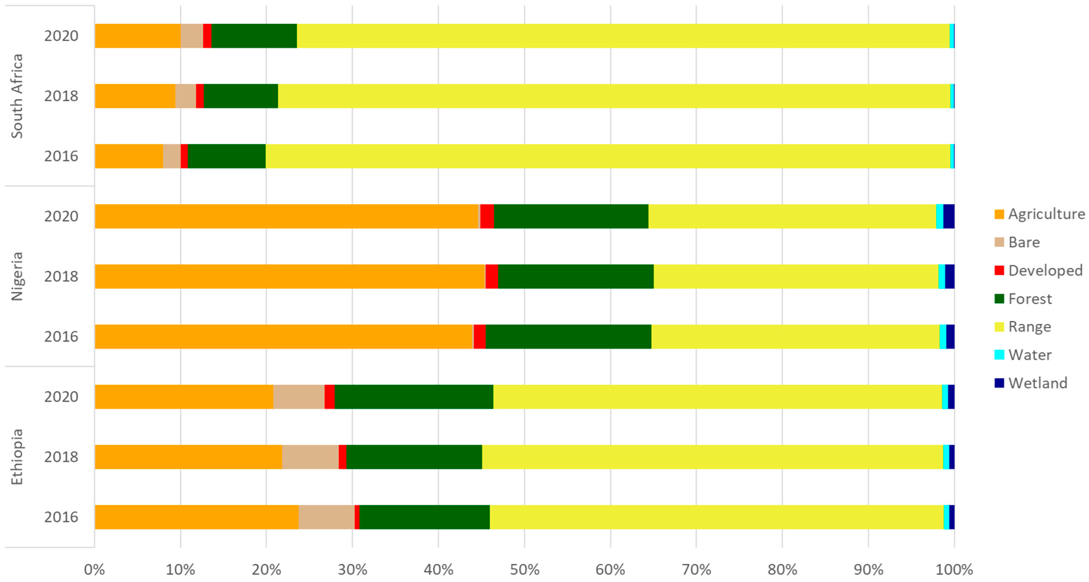
| Country | Year | Agriculture | Bare | Developed | Forest | Range | Water | Wetland |
|---|---|---|---|---|---|---|---|---|
| Ethiopia | 2016 | 23.7% | 6.5% | 0.5% | 15.2% | 52.8% | 0.6% | 0.6% |
| 2017 | 22.6% | 6.4% | 0.6% | 15.1% | 54.1% | 0.7% | 0.6% | |
| 2018 | 21.8% | 6.5% | 0.9% | 15.8% | 53.6% | 0.7% | 0.6% | |
| 2019 | 21.0% | 6.3% | 1.0% | 18.4% | 52.0% | 0.7% | 0.7% | |
| 2020 | 20.8% | 5.9% | 1.1% | 18.5% | 52.2% | 0.7% | 0.7% | |
| Nigeria | 2016 | 43.9% | 0.2% | 1.4% | 19.2% | 33.6% | 0.7% | 0.9% |
| 2017 | 45.3% | 0.3% | 1.3% | 17.4% | 34.1% | 0.7% | 0.9% | |
| 2018 | 45.3% | 0.2% | 1.4% | 18.1% | 33.1% | 0.8% | 1.1% | |
| 2019 | 45.4% | 0.2% | 1.5% | 18.1% | 32.7% | 0.8% | 1.3% | |
| 2020 | 44.6% | 0.3% | 1.5% | 18.0% | 33.5% | 0.8% | 1.3% | |
| South Africa | 2016 | 8.0% | 2.1% | 0.8% | 9.0% | 79.7% | 0.4% | 0.0% |
| 2017 | 8.8% | 2.2% | 0.8% | 8.9% | 78.8% | 0.4% | 0.1% | |
| 2018 | 9.4% | 2.4% | 0.9% | 8.7% | 78.2% | 0.4% | 0.1% | |
| 2019 | 9.4% | 2.5% | 0.9% | 8.8% | 77.9% | 0.4% | 0.1% | |
| 2020 | 10.0% | 2.6% | 1.0% | 9.9% | 76.0% | 0.4% | 0.1% |
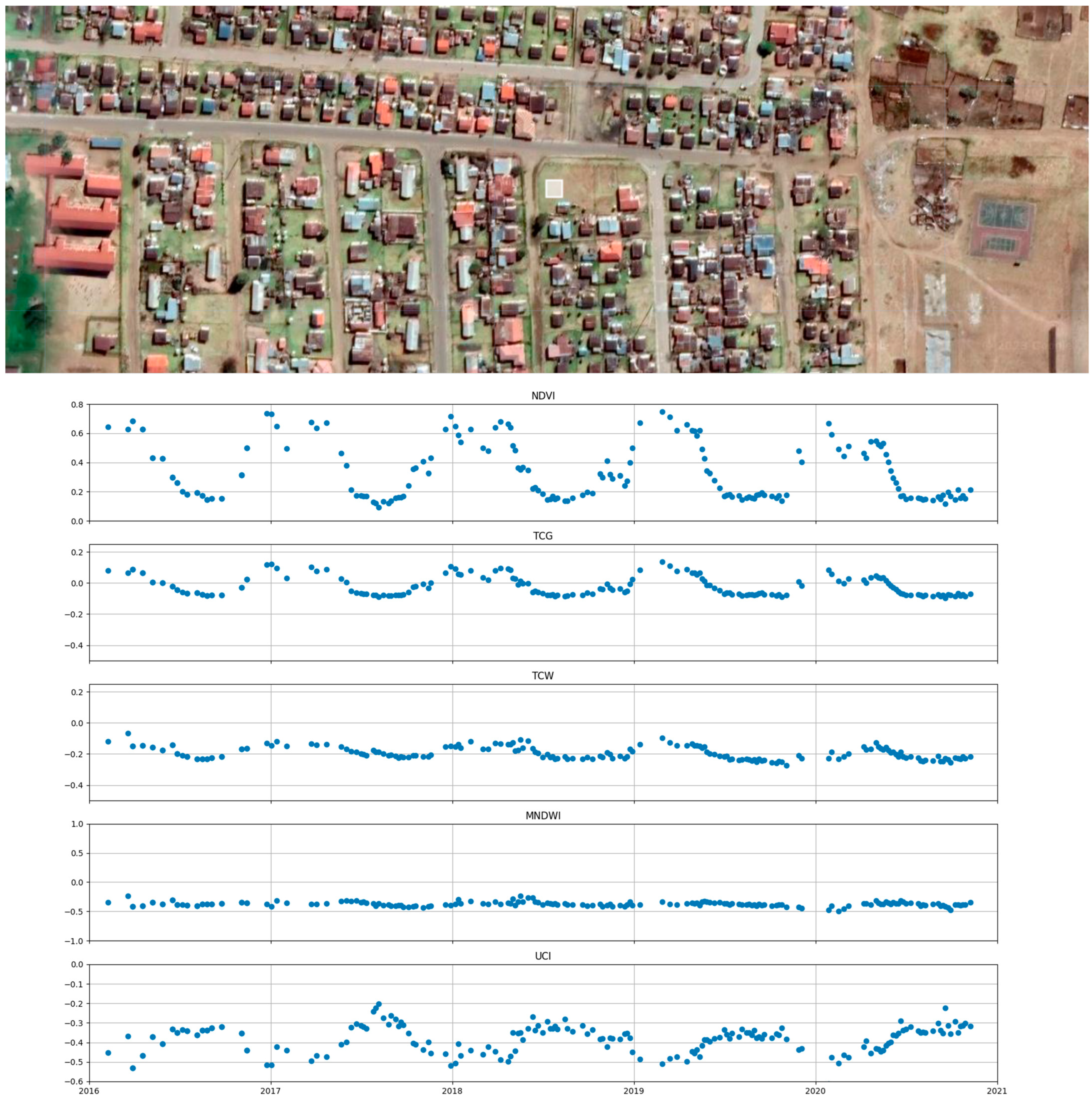
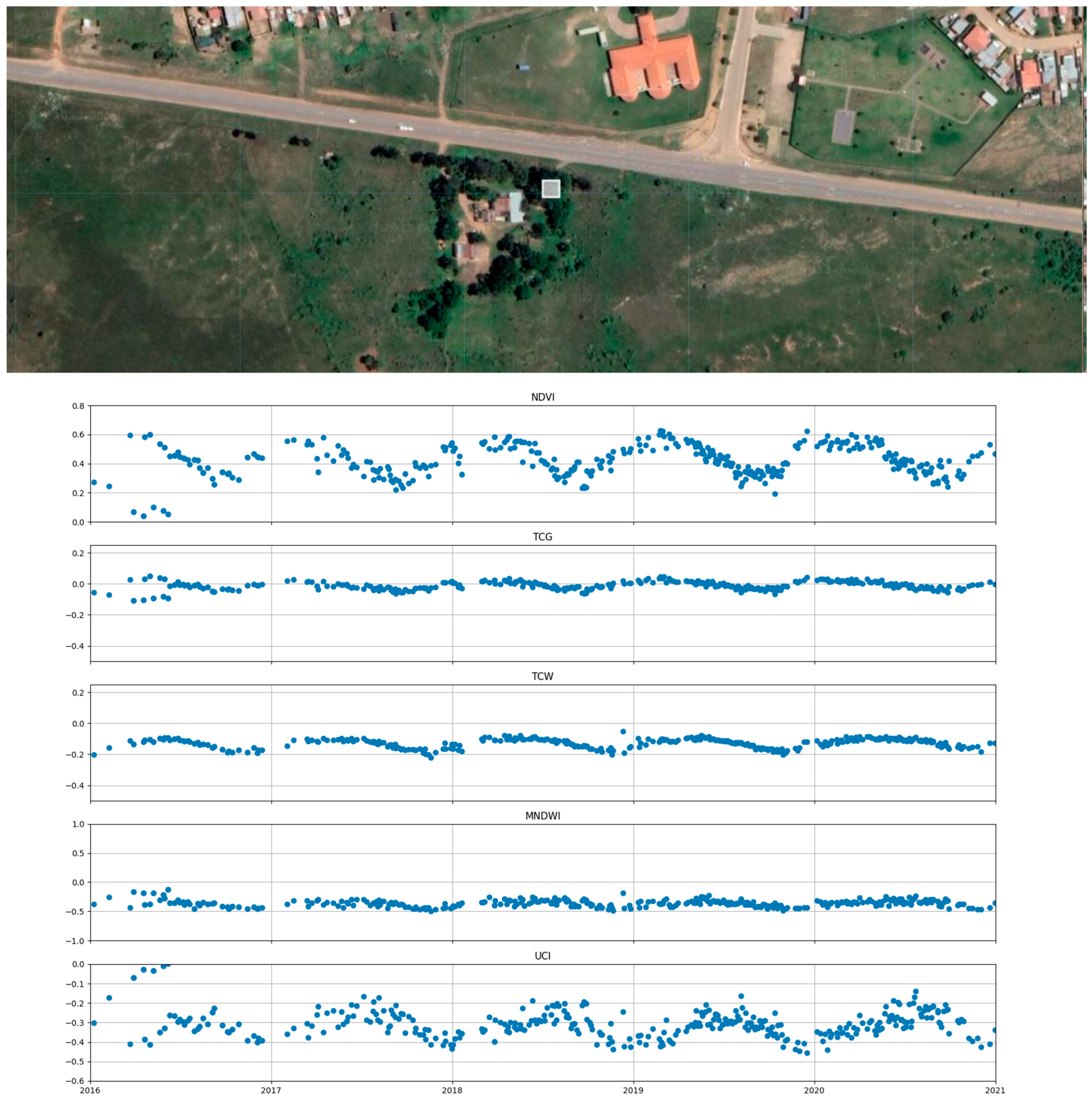
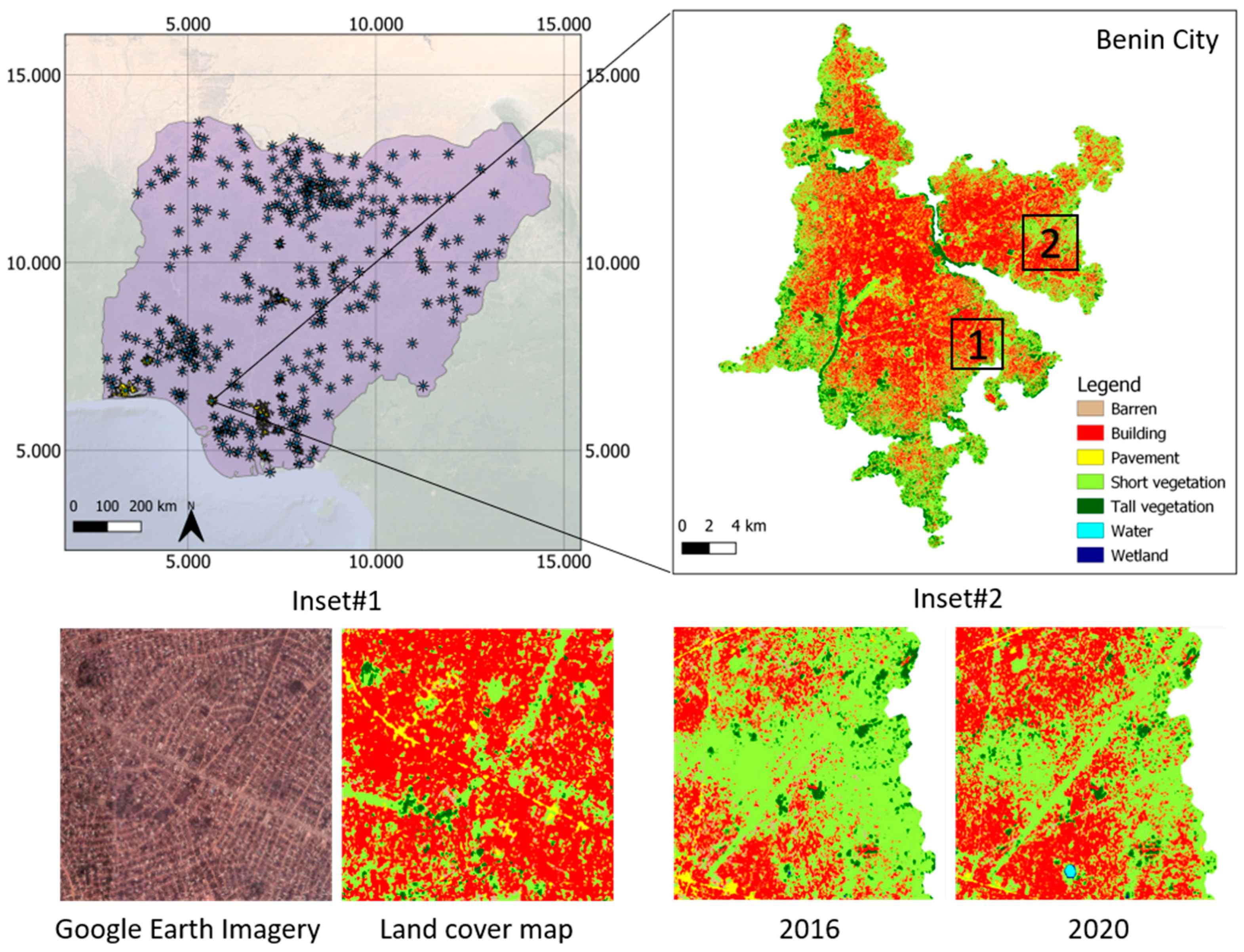
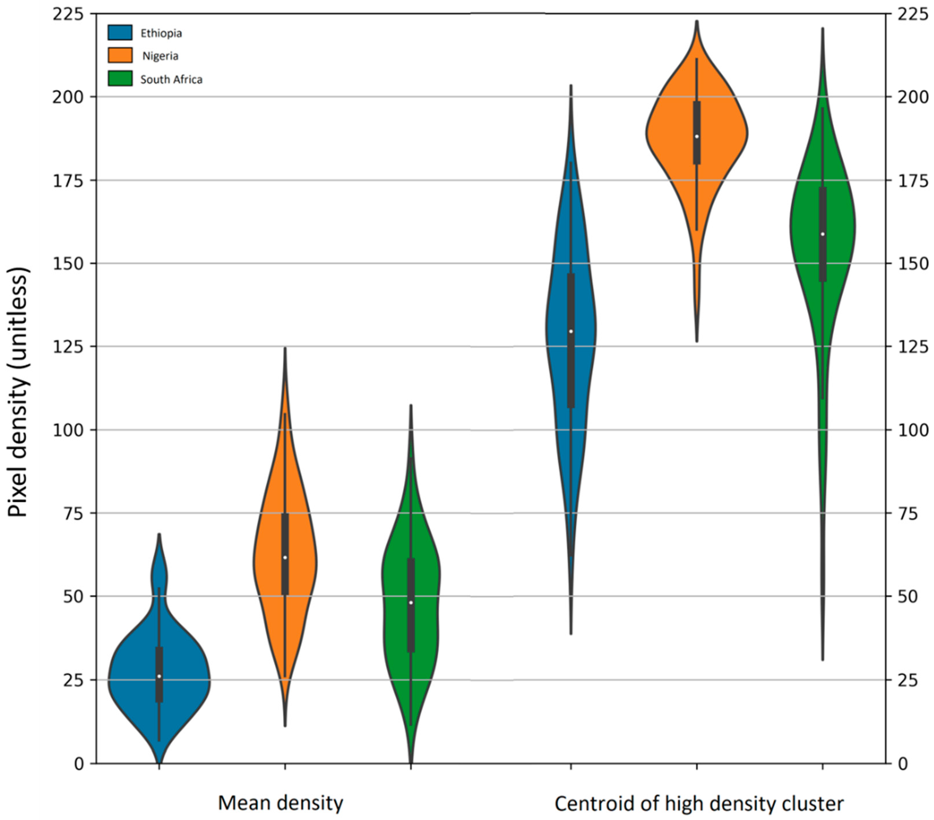
Appendix G. National Level Urban Agglomerations and Example Urban Land Covers
References
- United Nations; Department of Economic and Social Affairs; Population Division. World Urbanization Prospects: The 2018 Revision; United Nations: New York, NY, USA, 2019. [Google Scholar] [CrossRef]
- FAO; IFAD; UNICEF; WFP; WHO. The State of Food Security and Nutrition in the World 2023. In Urbanization, Agrifood Systems Transformation and Healthy Diets across the Rural–Urban Continuum; FAO: Rome, Italy, 2023. [Google Scholar] [CrossRef]
- World Bank Open Data. Available online: https://data.worldbank.org (accessed on 11 July 2024).
- Turok, I.; McGranahan, G. Urbanization and Economic Growth: The Arguments and Evidence for Africa and Asia. Environ. Urban. 2013, 25, 465–482. [Google Scholar] [CrossRef]
- Turok, I.; Borel-Saladin, J. Backyard Shacks, Informality and the Urban Housing Crisis in South Africa: Stopgap or Prototype Solution? Hous. Stud. 2016, 31, 384–409. [Google Scholar] [CrossRef]
- King, R.; Orloff, M.; Virsilas, T.; Pande, T. Confronting the Urban Housing Crisis in the Global South: Adequate, Secure, and Affordable Housing; World Resources Institute: Washington, DC, USA, 2017; Available online: https://www.wri.org/research/confronting-urban-housing-crisis-global-south-adequate-secure-and-affordable-housing (accessed on 11 July 2024).
- Parienté, W. Urbanization in Sub-Saharan Africa and the Challenge of Access to Basic Services. J. Demogr. Econ. 2017, 83, 31–39. [Google Scholar] [CrossRef]
- Güneralp, B.; Lwasa, S.; Masundire, H.; Parnell, S.; Seto, K.C. Urbanization in Africa: Challenges and Opportunities for Conservation. Environ. Res. Lett. 2017, 13, 15002. [Google Scholar] [CrossRef]
- Nathaniel, S.P.; Adeleye, N. Environmental Preservation amidst Carbon Emissions, Energy Consumption, and Urbanization in Selected African Countries: Implication for Sustainability. J. Clean. Prod. 2021, 285, 125409. [Google Scholar] [CrossRef]
- Arsiso, B.K.; Tsidu, G.M.; Stoffberg, G.H.; Tadesse, T. Influence of Urbanization-Driven Land Use/Cover Change on Climate: The Case of Addis Ababa, Ethiopia. Phys. Chem. Earth Parts A/B/C 2018, 105, 212–223. [Google Scholar] [CrossRef]
- Tiando, D.S.; Hu, S.; Fan, X.; Ali, M.R. Tropical Coastal Land-Use and Land Cover Changes Impact on Ecosystem Service Value during Rapid Urbanization of Benin, West Africa. Int. J. Environ. Res. Public Health 2021, 18, 7416. [Google Scholar] [CrossRef]
- McHale, M.R.; Bunn, D.N.; Pickett, S.T.A.; Twine, W. Urban Ecology in a Developing World: Why Advanced Socioecological Theory Needs Africa. Front. Ecol. Environ. 2013, 11, 556–564. [Google Scholar] [CrossRef] [PubMed]
- Li, X.; Chen, G.; Zhang, Y.; Yu, L.; Du, Z.; Hu, G.; Liu, X. The Impacts of Spatial Resolutions on Global Urban-Related Change Analyses and Modeling. iScience 2022, 25, 105660. [Google Scholar] [CrossRef]
- Sobrino, J.A.; Oltra-Carrió, R.; Sòria, G.; Bianchi, R.; Paganini, M. Impact of Spatial Resolution and Satellite Overpass Time on Evaluation of the Surface Urban Heat Island Effects. Remote Sens. Environ. 2012, 117, 50–56. [Google Scholar] [CrossRef]
- CCI; ESA. ESA CCI LAND COVER—S2 Prototype Land Cover 20m Map of Africa 2016. Available online: https://2016africalandcover20m.esrin.esa.int/ (accessed on 30 June 2024).
- Midekisa, A.; Holl, F.; Savory, D.J.; Andrade-Pacheco, R.; Gething, P.W.; Bennett, A.; Sturrock, H.J.W. Mapping Land Cover Change over Continental Africa Using Landsat and Google Earth Engine Cloud Computing. PLoS ONE 2017, 12, e0184926. [Google Scholar] [CrossRef] [PubMed]
- Feng, D.; Yu, L.; Zhao, Y.; Cheng, Y.; Xu, Y.; Li, C.; Gong, P. A Multiple Dataset Approach for 30-m Resolution Land Cover Mapping: A Case Study of Continental Africa. Int. J. Remote Sens. 2018, 39, 3926–3938. [Google Scholar] [CrossRef]
- Li, Q.; Qiu, C.; Ma, L.; Schmitt, M.; Zhu, X. Mapping the Land Cover of Africa at 10 m Resolution from Multi-Source Remote Sensing Data with Google Earth Engine. Remote Sens. 2020, 12, 602. [Google Scholar] [CrossRef]
- Cadenasso, M.L.; Pickett, S.T.A.; Schwarz, K. Spatial Heterogeneity in Urban Ecosystems: Reconceptualizing Land Cover and a Framework for Classification. Front. Ecol. Environ. 2007, 5, 80–88. [Google Scholar] [CrossRef]
- Prosperi, D.; Moudon, A.V.; Claessens, F. The Question of Metropolitan Form: Introduction. Footprint 2009, 3, 1–4. [Google Scholar] [CrossRef]
- Kemper, T.; Melchiorri, M.; Ehrlich, D. Global Human Settlement Layer; Publications Office of the European Union: Luxembourg, 2021. [Google Scholar] [CrossRef]
- Melchiorri, M.; Pesaresi, M.; Florczyk, A.J.; Corbane, C.; Kemper, T. Principles and Applications of the Global Human Settlement Layer as Baseline for the Land Use Efficiency Indicator—SDG 11.3. 1. ISPRS Int. J. Geoinf. 2019, 8, 96. [Google Scholar] [CrossRef]
- Schiavina, M.; Melchiorri, M.; Corbane, C.; Florczyk, A.; Freire, S.; Pesaresi, M.; Kemper, T. Multi-Scale Estimation of Land Use Efficiency (SDG 11.3.1) across 25 Years Using Global Open and Free Data. Sustainability 2019, 11, 5674. [Google Scholar] [CrossRef]
- Statista Africa: Total Population Forecast 2020–2050. Available online: https://www.statista.com/statistics/1224205/forecast-of-the-total-population-of-africa/ (accessed on 29 June 2024).
- World Economic Forum. African Cities Will Double in Population by 2050. Here Are 4 Ways to Make Sure They Thrive. Available online: https://www.weforum.org/agenda/2018/06/Africa-urbanization-cities-double-population-2050-4%20ways-thrive/ (accessed on 29 June 2024).
- Beck, H.E.; McVicar, T.R.; Vergopolan, N.; Berg, A.; Lutsko, N.J.; Dufour, A.; Zeng, Z.; Jiang, X.; Van Dijk, A.I.J.M.; Miralles, D.G. High-Resolution (1 Km) Köppen-Geiger Maps for 1901–2099 Based on Constrained CMIP6 Projections. Sci. Data 2023, 10, 724. [Google Scholar] [CrossRef] [PubMed]
- Woodcock, C.E.; Loveland, T.R.; Herold, M.; Bauer, M.E. Transitioning from Change Detection to Monitoring with Remote Sensing: A Paradigm Shift. Remote Sens. Environ. 2020, 238, 111558. [Google Scholar] [CrossRef]
- USGS. Landsat 4–7 Collection 2 Level 2 Science Product Guide U.S. Geological Survey. Available online: https://www.usgs.gov/media/files/landsat-4-7-collection-2-level-2-science-product-guide (accessed on 29 June 2024).
- USGS. Landsat 8–9 Collection 2 Level 2 Science Product Guide U.S. Geological Survey. Available online: https://www.usgs.gov/media/files/landsat-8-9-collection-2-level-2-science-product-guide (accessed on 29 June 2024).
- ESA. Sentinel-2 Products Specification Document. Available online: https://sentinels.copernicus.eu/documents/247904/0/Sentinel-2-product-specifications-document-V14-9.pdf (accessed on 29 June 2024).
- Google. Sentinel-2 Cloud Masking with S2cloudless. Available online: https://developers.google.com/earth-engine/tutorials/community/sentinel-2-s2cloudless (accessed on 30 June 2024).
- Kauth, R.J.; Thomas, G.S. The Tasselled-Cap—A Graphic Description of the Spectral-Temporal Development of Agricultural Crops as Seen by Landsat. Available online: https://docs.lib.purdue.edu/lars_symp/159 (accessed on 27 May 2024).
- Huang, S.; Tang, L.; Hupy, J.P.; Wang, Y.; Shao, G. A Commentary Review on the Use of Normalized Difference Vegetation Index (NDVI) in the Era of Popular Remote Sensing. J. For. Res. 2021, 32, 1–6. [Google Scholar] [CrossRef]
- Zhang, L.; Tian, Y.; Liu, Q. A Novel Urban Composition Index Based on Water-Impervious Surface-Pervious Surface (W-I-P) Model for Urban Compositions Mapping Using Landsat Imagery. Remote Sens. 2020, 13, 3. [Google Scholar] [CrossRef]
- Shahi, K.; Shafri, H.Z.M.; Taherzadeh, E.; Mansor, S.; Muniandy, R. A Novel Spectral Index to Automatically Extract Road Networks from WorldView-2 Satellite Imagery. Egypt. J. Remote Sens. Space Sci. 2015, 18, 27–33. [Google Scholar] [CrossRef]
- Javed, A.; Cheng, Q.; Peng, H.; Altan, O.; Li, Y.; Ara, I.; Huq, E.; Ali, Y.; Saleem, N. Review of Spectral Indices for Urban Remote Sensing. Photogramm. Eng. Remote Sens. 2021, 87, 513–524. [Google Scholar] [CrossRef]
- Xu, H. Modification of Normalised Difference Water Index (NDWI) to Enhance Open Water Features in Remotely Sensed Imagery. Int. J. Remote Sens. 2006, 27, 3025–3033. [Google Scholar] [CrossRef]
- Zhan, Z.; Qin, Q.; Ghulan, A.; Wang, D. NIR-Red Spectral Space Based New Method for Soil Moisture Monitoring. Sci. China Ser. D Earth Sci. 2007, 50, 283–289. [Google Scholar] [CrossRef]
- Gorelick, N.; Hancher, M.; Dixon, M.; Ilyushchenko, S.; Thau, D.; Moore, R. Google Earth Engine: Planetary-Scale Geospatial Analysis for Everyone. Remote Sens. Environ. 2017, 202, 18–27. [Google Scholar] [CrossRef]
- Haralick, R.M.; Shanmugam, K.; Dinstein, I. Textural Features for Image Classification. IEEE Trans. Syst. Man Cybern. 1973, SMC-3, 610–621. [Google Scholar] [CrossRef]
- Mastrorosa, S.; Crespi, M.; Congedo, L.; Munafò, M. Land Consumption Classification Using Sentinel 1 Data: A Systematic Review. Land 2023, 12, 932. [Google Scholar] [CrossRef]
- Mullissa, A.; Vollrath, A.; Odongo-Braun, C.; Slagter, B.; Balling, J.; Gou, Y.; Gorelick, N.; Reiche, J. Sentinel-1 SAR Backscatter Analysis Ready Data Preparation in Google Earth Engine. Remote Sens. 2021, 13, 1954. [Google Scholar] [CrossRef]
- Mills, S.; Weiss, S.; Liang, C. VIIRS Day/Night Band (DNB) Stray Light Characterization and Correction. Earth Obs. Syst. XVIII 2013, 8866, 549–566. [Google Scholar] [CrossRef]
- Fick, S.E.; Hijmans, R.J. WorldClim 2: New 1-km Spatial Resolution Climate Surfaces for Global Land Areas. Int. J. Climatol. 2017, 37, 4302–4315. [Google Scholar] [CrossRef]
- Abatzoglou, J.T.; Dobrowski, S.Z.; Parks, S.A.; Hegewisch, K.C. TerraClimate, a High-Resolution Global Dataset of Monthly Climate and Climatic Water Balance from 1958–2015. Sci. Data 2018, 5, 170191. [Google Scholar] [CrossRef]
- Theobald, D.M.; Harrison-Atlas, D.; Monahan, W.B.; Albano, C.M. Ecologically-Relevant Maps of Landforms and Physiographic Diversity for Climate Adaptation Planning. PLoS ONE 2015, 10, e0143619. [Google Scholar] [CrossRef] [PubMed]
- Hengl, T.; Miller, M.A.E.; Križan, J.; Shepherd, K.D.; Sila, A.; Kilibarda, M.; Antonijević, O.; Glušica, L.; Dobermann, A.; Haefele, S.M.; et al. African Soil Properties and Nutrients Mapped at 30 m Spatial Resolution Using Two-Scale Ensemble Machine Learning. Sci. Rep. 2021, 11, 6130. [Google Scholar] [CrossRef]
- Dinerstein, E.; Olson, D.; Joshi, A.; Vynne, C.; Burgess, N.D.; Wikramanayake, E.; Hahn, N.; Palminteri, S.; Hedao, P.; Noss, R.; et al. An Ecoregion-Based Approach to Protecting Half the Terrestrial Realm. Bioscience 2017, 67, 534–545. [Google Scholar] [CrossRef]
- Stehman, S.V. Estimating Area and Map Accuracy for Stratified Random Sampling When the Strata Are Different from the Map Classes. Int. J. Remote Sens. 2014, 35, 4923–4939. [Google Scholar] [CrossRef]
- Braaten, J. GitHub—Jdbcode/Ee-Rgb-Timeseries: Earth Engine JS Module to Color Time Series Chart Points as Stretched 3-Band RGB. Available online: https://github.com/jdbcode/ee-rgb-timeseries (accessed on 30 June 2024).
- Oregon State University. GitHub—EMapR/TimeSync-Plus: An Application for Gathering Point and Polygon Spectral Temporal Information from Landsat Time Series Data into a Database. Available online: https://github.com/eMapR/TimeSync-Plus (accessed on 30 June 2024).
- Belgiu, M.; Drăguţ, L. Random Forest in Remote Sensing: A Review of Applications and Future Directions. ISPRS J. Photogramm. Remote Sens. 2016, 114, 24–31. [Google Scholar] [CrossRef]
- Sheykhmousa, M.; Mahdianpari, M.; Ghanbari, H.; Mohammadimanesh, F.; Ghamisi, P.; Homayouni, S. Support Vector Machine versus Random Forest for Remote Sensing Image Classification: A Meta-Analysis and Systematic Review. IEEE J. Sel. Top. Appl. Earth Obs. Remote Sens. 2020, 13, 6308–6325. [Google Scholar] [CrossRef]
- Adugna, T.; Xu, W.; Fan, J. Comparison of Random Forest and Support Vector Machine Classifiers for Regional Land Cover Mapping Using Coarse Resolution FY-3C Images. Remote Sens. 2022, 14, 574. [Google Scholar] [CrossRef]
- Strobl, C.; Boulesteix, A.-L.; Kneib, T.; Augustin, T.; Zeileis, A. Conditional Variable Importance for Random Forests. BMC Bioinform. 2008, 9, 307. [Google Scholar] [CrossRef]
- Cardenas-Ritzert, O.S.E.; Vogeler, J.C.; Shah Heydari, S.; Fekety, P.A.; Laituri, M.; McHale, M. Automated Geospatial Approach for Assessing SDG Indicator 11.3.1: A Multi-Level Evaluation of Urban Land Use Expansion across Africa. ISPRS Int. J. Geoinf. 2024, 13, 226. [Google Scholar] [CrossRef]
- McGarigal, K.; Marks, B.J. FRAGSTATS: Spatial Pattern Analysis Program for Quantifying Landscape Structure; US Department of Agriculture, Forest Service, Pacific Northwest Research Station: Portland, OR, USA, 1995. [CrossRef]
- Prakash, P.S.; Nimish, G.; Chandan, M.C.; Bharath, H.A. Urbanization: Pattern, Effects and Modelling. In Machine Learning Approaches for Urban Computing; Bandyopadhyay, M., Rout, M., Chandra Satapathy, S., Eds.; Springer: Singapore, 2021; Volume 968, pp. 1–21. ISBN 9789811609343/9789811609350. [Google Scholar]
- Guan, J.; Wang, R.; Van Berkel, D.; Liang, Z. How Spatial Patterns Affect Urban Green Space Equity at Different Equity Levels: A Bayesian Quantile Regression Approach. Landsc. Urban Plan. 2023, 233, 104709. [Google Scholar] [CrossRef]
- Gong, P.; Liu, H.; Zhang, M.; Li, C.; Wang, J.; Huang, H.; Clinton, N.; Ji, L.; Li, W.; Bai, Y.; et al. Stable Classification with Limited Sample: Transferring a 30-m Resolution Sample Set Collected in 2015 to Mapping 10-m Resolution Global Land Cover in 2017. Sci. Bull. 2019, 64, 370–373. [Google Scholar] [CrossRef] [PubMed]
- Tsendbazar, N.; Herold, M.; Li, L.; Tarko, A.; De Bruin, S.; Masiliunas, D.; Lesiv, M.; Fritz, S.; Buchhorn, M.; Smets, B.; et al. Towards Operational Validation of Annual Global Land Cover Maps. Remote Sens. Environ. 2021, 266, 112686. [Google Scholar] [CrossRef]
- ESA. WorldCover Product User Manual. Available online: https://esa-worldcover.s3.eu-central-1.amazonaws.com/v200/2021/docs/WorldCover_PUM_V2.0.pdf (accessed on 29 June 2024).
- Huang, H.; Li, Q.; Zhang, Y. A High-Resolution Remote-Sensing-Based Method for Urban Ecological Quality Evaluation. Front. Environ. Sci. 2022, 10, 765604. [Google Scholar] [CrossRef]
- Milošević, R.; Šiljeg, S.; Marić, I. WorldView-3 Imagery and GEOBIA Method for the Urban Land Use Pattern Analysis: Case Study City of Split, Croatia. In Geographical Information Systems Theory, Applications and Management; Springer: Cham, Switzerland, 2023; pp. 52–67. [Google Scholar] [CrossRef]
- Karra, K.; Kontgis, C.; Statman-Weil, Z.; Mazzariello, J.C.; Mathis, M.; Brumby, S.P. Global Land Use / Land Cover with Sentinel 2 and Deep Learning. In Proceedings of the 2021 IEEE International Geoscience and Remote Sensing Symposium IGARSS, Brussels, Belgium, 11–16 July 2021; pp. 4704–4707. [Google Scholar] [CrossRef]
- Malinowski, R.; Lewiński, S.; Rybicki, M.; Gromny, E.; Jenerowicz, M.; Krupiński, M.; Nowakowski, A.; Wojtkowski, C.; Krupiński, M.; Krätzschmar, E.; et al. Automated Production of a Land Cover/Use Map of Europe Based on Sentinel-2 Imagery. Remote Sens. 2020, 12, 3523. [Google Scholar] [CrossRef]
- Benhammou, Y.; Alcaraz-Segura, D.; Guirado, E.; Khaldi, R.; Boujemâa, A.; Herrera, F.; Tabik, S. Sentinel2GlobalLULC: A Deep-Learning-Ready Sentinel-2 RGB Image Dataset for Global Land Use/Cover Mapping. bioRxiv 2021. [Google Scholar] [CrossRef]
- Zhang, X.; Liu, L.; Chen, X.; Gao, Y.; Xie, S.; Mi, J. GLC_FCS30: Global Land-Cover Product with Fine Classification System at 30 m Using Time-Series Landsat Imagery. Earth Syst. Sci. Data 2021, 13, 2753–2776. [Google Scholar] [CrossRef]
- Abercrombie, P.; Friedl, M.A. Improving the Consistency of Multitemporal Land Cover Maps Using a Hidden Markov Model. IEEE Trans. Geosci. Remote Sens. 2016, 54, 703–713. [Google Scholar] [CrossRef]
- Copernicus Global Land Service Dynamic Land Cover. Available online: https://land.copernicus.eu/en/products/global-dynamic-land-cover (accessed on 30 June 2024).
- European Space Agency (ESA) Land Cover CCI Product User Guide Version 2. Tech. Rep. Available online: https://www.google.com.hk/url?sa=t&source=web&rct=j&opi=89978449&url=https://maps.elie.ucl.ac.be/CCI/viewer/download/ESACCI-LC-Ph2-PUGv2_2.0.pdf&ved=2ahUKEwi4h9K72LeHAxWodPUHHWQNMQkQFnoECBYQAQ&usg=AOvVaw2qA1Mgwlt6Vm3yN8OKvYe4 (accessed on 30 June 2024).
- United Nations Human Settlements Programme. Urban Sustainable Development Goals (SDGs). Available online: https://data.unhabitat.org/pages/sdgs (accessed on 30 June 2024).
- Ludwig, C.; Hecht, R.; Lautenbach, S.; Schorcht, M.; Zipf, A. Mapping Public Urban Green Spaces Based on Openstreetmap and Sentinel-2 Imagery Using Belief Functions. ISPRS Int. J. Geoinf. 2021, 10, 251. [Google Scholar] [CrossRef]
- Kopecká, M.; Szatmári, D.; Rosina, K. Analysis of Urban Green Spaces Based on Sentinel-2A: Case Studies from Slovakia. Land 2017, 6, 25. [Google Scholar] [CrossRef]
- Mohan, M.; Kikegawa, Y.; Gurjar, B.R.; Bhati, S.; Kolli, N.R. Assessment of Urban Heat Island Effect for Different Land Use–Land Cover from Micrometeorological Measurements and Remote Sensing Data for Megacity Delhi. Theor. Appl. Climatol. 2013, 112, 647–658. [Google Scholar] [CrossRef]
- Shrestha, M.K.; York, A.M.; Boone, C.G.; Zhang, S. Land Fragmentation Due to Rapid Urbanization in the Phoenix Metropolitan Area: Analyzing the Spatiotemporal Patterns and Drivers. Appl. Geogr. 2012, 32, 522–531. [Google Scholar] [CrossRef]
- Haas, J.; Ban, Y. Urban Land Cover and Ecosystem Service Changes Based on Sentinel-2A MSI and Landsat TM Data. IEEE J. Sel. Top. Appl. Earth Obs. Remote Sens. 2018, 11, 485–497. [Google Scholar] [CrossRef]
- Guilherme, F.; Gonçalves, J.A.; Carretero, M.A.; Farinha-Marques, P. Assessment of Land Cover Trajectories as an Indicator of Urban Habitat Temporal Continuity. Landsc. Urban Plan. 2024, 242, 104932. [Google Scholar] [CrossRef]
- Alexander, C. Influence of the Proportion, Height and Proximity of Vegetation and Buildings on Urban Land Surface Temperature. Int. J. Appl. Earth Obs. Geoinf. 2021, 95, 102265. [Google Scholar] [CrossRef]
- Duncan, J.M.A.; Boruff, B.; Saunders, A.; Sun, Q.; Hurley, J.; Amati, M. Turning down the Heat: An Enhanced Understanding of the Relationship between Urban Vegetation and Surface Temperature at the City Scale. Sci. Total Environ. 2019, 656, 118–128. [Google Scholar] [CrossRef] [PubMed]
- Perini, K.; Magliocco, A. Effects of Vegetation, Urban Density, Building Height, and Atmospheric Conditions on Local Temperatures and Thermal Comfort. Urban. For. Urban Green. 2014, 13, 495–506. [Google Scholar] [CrossRef]
- Yu, Q.; Acheampong, M.; Pu, R.; Landry, S.M.; Ji, W.; Dahigamuwa, T. Assessing Effects of Urban Vegetation Height on Land Surface Temperature in the City of Tampa, Florida, USA. Int. J. Appl. Earth Obs. Geoinf. 2018, 73, 712–720. [Google Scholar] [CrossRef]
- Lauwaet, D.; Hooyberghs, H.; Maiheu, B.; Lefebvre, W.; Driesen, G.; Van Looy, S.; De Ridder, K. Detailed Urban Heat Island Projections for Cities Worldwide: Dynamical Downscaling CMIP5 Global Climate Models. Climate 2015, 3, 391–415. [Google Scholar] [CrossRef]
- Simwanda, M.; Ranagalage, M.; Estoque, R.C.; Murayama, Y. Spatial Analysis of Surface Urban Heat Islands in Four Rapidly Growing African Cities. Remote Sens. 2019, 11, 1645. [Google Scholar] [CrossRef]
- Rakhshandehroo, M.; Yusof, M.J.M.; Arabi, R.; Parva, M.; Nochian, A. The Environmental Benefits of Urban Open Green Spaces. Alam Cipta 2017, 10, 10–16. [Google Scholar]
- Lee, A.C.K.; Maheswaran, R. The Health Benefits of Urban Green Spaces: A Review of the Evidence. J. Public Health 2011, 33, 212–222. [Google Scholar] [CrossRef] [PubMed]
- Cetin, M. Using GIS Analysis to Assess Urban Green Space in Terms of Accessibility: Case Study in Kutahya. Int. J. Sustain. Dev. World Ecol. 2015, 22, 420–424. [Google Scholar] [CrossRef]
- Cheng, X.; Zhang, N.; Xie, W.; Cai, G. Method of Accessing the Urban Public Space from GF-2 Image by Indicator SDG 11.7.1. In Proceedings of the IGARSS 2022—2022 IEEE International Geoscience and Remote Sensing Symposium, Kuala Lumpur, Malaysia, 17–22 July 2022; pp. 4353–4356. [Google Scholar]
- Stumpf, A.; Michéa, D.; Malet, J.-P. Improved Co-Registration of Sentinel-2 and Landsat-8 Imagery for Earth Surface Motion Measurements. Remote Sens. 2018, 10, 160. [Google Scholar] [CrossRef]
- McHale, M.R.; Beck, S.M.; Pickett, S.T.A.; Childers, D.L.; Cadenasso, M.L.; Rivers, L.; Swemmer, L.; Ebersohn, L.; Twine, W.; Bunn, D.N. Democratization of Ecosystem Services—A Radical Approach for Assessing Nature’s Benefits in the Face of Urbanization. Ecosyst. Health Sustain. 2018, 4, 115–131. [Google Scholar] [CrossRef]
- Crist, E.P. A TM Tasseled Cap Equivalent Transformation for Reflectance Factor Data. Remote Sens. Environ. 1985, 17, 301–306. [Google Scholar] [CrossRef]
- Shi, T.; Xu, H. Derivation of Tasseled Cap Transformation Coefficients for Sentinel-2 MSI At-Sensor Reflectance Data. IEEE J. Sel. Top. Appl. Earth Obs. Remote Sens. 2019, 12, 4038–4048. [Google Scholar] [CrossRef]
- Worldclim. Worldclim Biometric Variables. Available online: https://www.worldclim.org/data/bioclim.html (accessed on 11 July 2024).


| Country | Area (km2) | Population (in Millions); (% Growth Rate/Year) | Real Gross Domestic Product (GDP—Annual % Growth) |
|---|---|---|---|
| Ethiopia | 1.1 million | 123.4 (2.4–2.5) | 6.2 |
| Nigeria | 0.9 million | 218.5 (2.4–2.5) | 3.1 |
| South Africa | 1.2 million | 59.9 (0.8) | 1.8 |
| Imagery Details | |||
|---|---|---|---|
| Sensor Type/Dataset | Tier 1 Land Use Products | Tier 2 Land Cover Products | Derived Features |
| Optical | Landsat Collection-2 Surface Reflectance @ 30 m, six bands of Blue, Green, Red, NIR, SWIR1, and SWIR2
| Sentinel-2 Top of Atmosphere * @ 10 m, six bands of B2(blue), B3(green), B4(red), B8(NIR), B11(SWIR1), B12(SWIR2)
|
GLCM metrics of ASM, Contrast, Correlation, Variance, Sum average, Entropy, Information Measures of correlation (1 and 2), Dissimilarity, Cluster shade, and Cluster prominence |
| Synthetic Aperture Radar | Sentinel-1 SAR Ground Range Detected VV polarization ** @ 30 m
| Sentinel-1 SAR Ground Range Detected VV polarization @ 10 m
| |
| Visible Infrared Imaging Radiometer Suite (VIIRS) Day/Night Band (DNB) @ 460 m | Included | Included | Yearly median of average monthly radiance values (months with at least two observations are counted) |
| TerraClimate @1/24 degree (~4.5 km) | Not included | Included | Total year precipitation and yearly minimum/maximum temperature |
| WorldClim V2.1 @ 30 arcseconds (~1 km) | Included | Included | 19 bioclimatic variables (bio_01 to bio_19) featuring normal (30 years) temperature and precipitation statistics, as defined in Appendix A |
| SRTM digital elevation data @ 30 m | Included | Included | Terrain parameter (elevation, slope, aspect)—static parameter |
| Continuous Heat-Insolation Load Index (CHILI_Index) @ 90 m | Included | Included | CHILI index (a number between 0 and 255) |
| iSDA soil texture class @ 30 m | Included | Included | USDA Texture Class at 0–20 cm depth (a number from 0 to 12) |
| World Ecoregions (RESOLVE), vector dataset | Included | Included | Ecoregion identifier (a 3-digit number) |
| Country | Tier | Training Pixels | Validation Pixels |
|---|---|---|---|
| Ethiopia | Tier 1, whole country | 740 | 550 |
| Tier 2, final urban agglomerations | 1172 | 700 | |
| Nigeria | Tier 1, whole country | 687 | 700 |
| Tier 2, final urban agglomerations | 1200 | 525 | |
| South Africa | Tier 1, whole country | 957 | 1000 |
| Tier 2, final urban agglomerations | 2897 | 1050 |
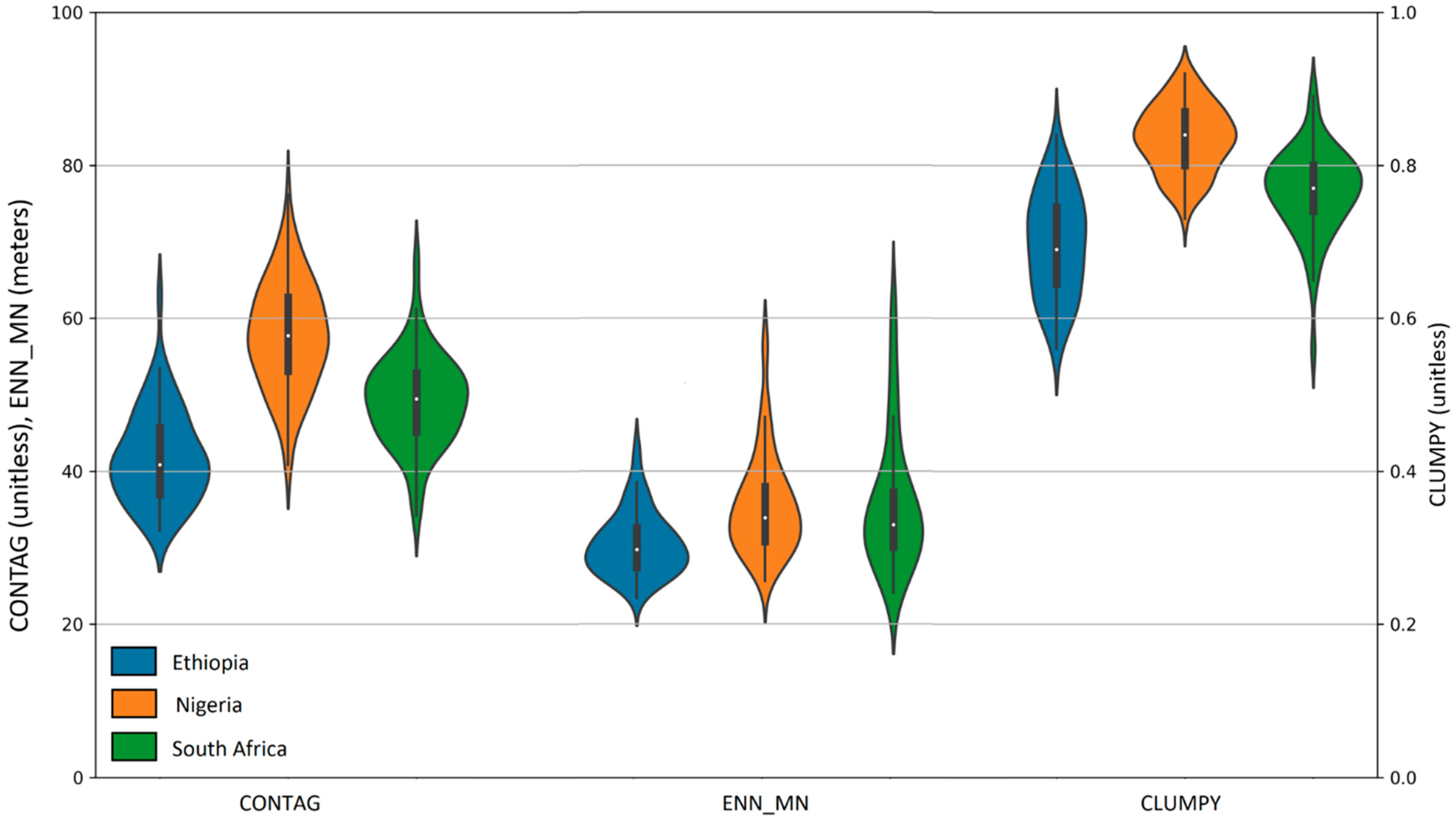
| Metric Name | Symbol Definition | Purpose |
|---|---|---|
| Contagion index | CONTAG | Spatial distribution (dispersion) and mixing (interspersion) of all land cover classes |
| Clumpiness index | CLUMP | Level of aggregation (clumpiness), calculated for building land cover |
| Euclidean nearest neighbor distance—Mean | ENN_MN | Mean of Euclidean nearest-neighbor distance, calculated for vegetation land cover |
| Ethiopia | Nigeria | South Africa | |||||||
|---|---|---|---|---|---|---|---|---|---|
| Class | Map UA | Map PA | Map F1 | Map UA | Map PA | Map F1 | Map UA | Map PA | Map F1 |
| Agriculture | 61.2 | 77.0 | 68.2 | 72.4 | 77.4 | 74.8 | 64.7 | 89.9 | 75.3 |
| Bare | 45.5 | 95.8 | 61.7 | 81.0 | 27.9 | 41.5 | 53.7 | 6.9 | 12.2 |
| Developed | 33.1 | 23.4 | 27.4 | 81.5 | 47.8 | 60.3 | 92.0 | 24.1 | 38.2 |
| Forest | 76.4 | 80.2 | 78.3 | 62.7 | 59.0 | 60.8 | 53.7 | 82.9 | 65.1 |
| Range | 86.4 | 72.0 | 78.5 | 57.9 | 57.4 | 57.6 | 77.4 | 88.5 | 82.6 |
| Water | 96.7 | 100.0 | 98.3 | 75.3 | 92.9 | 83.2 | 86.3 | 98.8 | 92.1 |
| Wetland | 57.7 | 64.7 | 61.0 | 78.3 | 49.7 | 60.8 | 67.6 | 8.3 | 14.8 |
| Map OA | 95% CI | Map OA | 95% CI | Map OA | 95% CI | ||||
| 74.6 | 7.3 | 65.9 | 5.4 | 73.6 | 6.8 | ||||
| Ethiopia | Nigeria | South Africa | |||||||
|---|---|---|---|---|---|---|---|---|---|
| Class | Map UA | Map PA | Map F1 | Map UA | Map PA | Map F1 | Map UA | Map PA | Map F1 |
| Barren | 40.1 | 60.4 | 48.2 | 66.9 | 31.8 | 43.1 | 68.8 | 36.4 | 47.6 |
| Building | 68.1 | 55.6 | 61.2 | 58.4 | 85.2 | 69.3 | 48.0 | 85.8 | 61.5 |
| Pavement | 29.3 | 63.1 | 40.0 | 66.2 | 26.9 | 38.3 | 46.1 | 41.7 | 43.8 |
| Short vegetation | 89.8 | 85.7 | 87.7 | 75.2 | 74.3 | 74.7 | 85.4 | 67.5 | 75.4 |
| Tall vegetation | 62.7 | 63.2 | 63.0 | 65.7 | 70.1 | 67.8 | 46.5 | 55.9 | 50.8 |
| Water | 96.7 | 95.8 | 96.3 | 90.0 | 96.4 | 93.1 | 77.5 | 82.3 | 79.8 |
| Wetland | 52.3 | 58.8 | 55.4 | 86.8 | 58.9 | 70.2 | 16.9 | 90.2 | 28.4 |
| Map OA | 95% CI | Map OA | 95% CI | Map OA | 95% CI | ||||
| 78.3 | 5.1 | 66.3 | 5.3 | 62.8 | 3.7 | ||||
| Developed (2016) | Net Conversion from Other Land Uses from 2016 to 2020 | Developed (2020) | Absolute Change | Relative Change | ||||||
|---|---|---|---|---|---|---|---|---|---|---|
| Agriculture | Bare | Forest | Rangeland | Water | Wetland | |||||
| Ethiopia | 153,779 | 54,029 | 16 | 3066 | 19,635 | 2 | 57 | 230,584 | 76,805 | 49.9% |
| Nigeria | 658,438 | 89,162 | 0 | 22,940 | 15,839 | −36 | 97 | 786,440 | 128,002 | 19.4% |
| South Africa | 635,139 | 1790 | 664 | 3955 | 75,892 | −3 | 26 | 717,463 | 82,324 | 13.0% |
| Country | Year | CONTAG (Unitless) | CLUMP (Building Class, Unitless) | ENN MN (Vegetation Class, Meters) |
|---|---|---|---|---|
| Ethiopia | 2016 | 39, 31–52 | 0.7, 0.58–0.83 | 32, 25–43 |
| 2020 | 41, 32–53 | 0.7, 0.56–0.84 | 30, 23–43 | |
| Nigeria | 2016 | 58, 39–82 | 0.85, 0.76–0.92 | 38, 27–58 |
| 2020 | 58, 41–76 | 0.83, 0.73–0.92 | 35, 26–57 | |
| South Africa | 2016 | 47, 32–64 | 0.75, 0.57–0.86 | 38, 25–65 |
| 2020 | 49, 34–67 | 0.76, 0.56–0.89 | 36, 24–62 |
Disclaimer/Publisher’s Note: The statements, opinions and data contained in all publications are solely those of the individual author(s) and contributor(s) and not of MDPI and/or the editor(s). MDPI and/or the editor(s) disclaim responsibility for any injury to people or property resulting from any ideas, methods, instructions or products referred to in the content. |
© 2024 by the authors. Licensee MDPI, Basel, Switzerland. This article is an open access article distributed under the terms and conditions of the Creative Commons Attribution (CC BY) license (https://creativecommons.org/licenses/by/4.0/).
Share and Cite
Shah Heydari, S.; Vogeler, J.C.; Cardenas-Ritzert, O.S.E.; Filippelli, S.K.; McHale, M.; Laituri, M. Multi-Tier Land Use and Land Cover Mapping Framework and Its Application in Urbanization Analysis in Three African Countries. Remote Sens. 2024, 16, 2677. https://doi.org/10.3390/rs16142677
Shah Heydari S, Vogeler JC, Cardenas-Ritzert OSE, Filippelli SK, McHale M, Laituri M. Multi-Tier Land Use and Land Cover Mapping Framework and Its Application in Urbanization Analysis in Three African Countries. Remote Sensing. 2024; 16(14):2677. https://doi.org/10.3390/rs16142677
Chicago/Turabian StyleShah Heydari, Shahriar, Jody C. Vogeler, Orion S. E. Cardenas-Ritzert, Steven K. Filippelli, Melissa McHale, and Melinda Laituri. 2024. "Multi-Tier Land Use and Land Cover Mapping Framework and Its Application in Urbanization Analysis in Three African Countries" Remote Sensing 16, no. 14: 2677. https://doi.org/10.3390/rs16142677