Article

Advantages of High-Temporal L-Band SAR Observations for Estimating Active Landslide Dynamics: A Case Study of the Kounai Landslide in Sobetsu Town, Hokkaido, Japan

by
Seiya Usami
1,2,*,
Satoshi Ishimaru
1 and
Takeo Tadono
2,3
1
Hokkaido Research Organization, Kita 19, Nishi 12, Kita-ku, Sapporo 060-0819, Hokkaido, Japan
2
Graduate School of Information Science and Technology, Hokkaido University, Kita 14, Nishi 9, Kita-ku, Sapporo 060-0814, Hokkaido, Japan
3
Earth Observation Research Center, Japan Aerospace Exploration Agency, 2-1-1 Sengen, Tsukuba 305-8505, Ibaraki, Japan
*
Author to whom correspondence should be addressed.
Remote Sens. 2024, 16(15), 2687; https://doi.org/10.3390/rs16152687 (registering DOI)
Submission received: 4 June 2024 / Revised: 14 July 2024 / Accepted: 17 July 2024 / Published: 23 July 2024
(This article belongs to the Special Issue Monitoring Geohazard from Synthetic Aperture Radar Interferometry)

Abstract

:
Estimating landslide dynamics is vital for the prevention of landslide disasters. Differential interferometric synthetic aperture radar (DInSAR) based on L-band SAR satellites is an effective tool for estimating the dynamics of forested landslides that occur in Japan. High-temporal L-band SAR observations have been planned for the future. Thus, it is necessary to further investigate the specific advantages of high-temporal L-band SAR observations for estimating landslide dynamics. In this study, we used DInSAR data with different time windows to identify active landslides in Hokkaido, Japan. This study is the first attempt to demonstrate the advantages of high-temporal L-band SAR observations for estimating active landslide dynamics. We successfully observed the dynamics of two active landslides, Kounai-1 and Kounai-2, using DInSAR over a time window of 14 days. We present the first spatial observation of the dynamics of Kounai-1 and Kounai-2. In addition, we discuss the dynamics of Kounai-1 and Kounai-2 based on interferograms, and our results suggest that both landslides are subunits of the same landslide, called the Kounai landslide. These results indicate that high-temporal L-band SAR observations can mitigate cycle slips and enable the estimation of active landslide dynamics.

1. Introduction

Landslides (i.e., slides [1]) are one of the mass movements that occur along one or several sliding surfaces [1]. They occur when slopes become unstable owing to rainfall [2], snowmelt [3], river erosion [4], earthquake [5], and artificial influence [6]. In regions with humid climate and variable geological zones, such as Japan, landslides pose a significant risk to societal infrastructure, such as roads [7]. Landslide Terrain Data Maps (LTDMs) have been developed in Japan, e.g., by [8,9,10], based on aerial photograph interpretations, which are crucial for assessing landslide disaster risk [11]. However, it is difficult to quantitatively understand landslide dynamics by interpreting aerial photographs. Therefore, the LTDM’s assessment of landslide disaster risk has limitations. For instance, a landslide event occurred in May 2022 in Nagano Prefecture, Japan, without prior anticipation of landslide dynamics, leading to an inability to forecast slope failures caused by landslide movement [12]. Thus, to thoroughly and quantitatively assess landslide disaster risk, it is imperative to evaluate the landslide dynamics within the LTDM [13].
Differential interferometric synthetic aperture radar (DInSAR) is based on the phase difference of electromagnetic waves at two epochs observed by a space-borne SAR. DInSAR is effective for spatially monitoring ground motion dynamics, such as earthquakes, e.g., by [14,15,16]; volcanoes, e.g., by [17,18,19]; ground subsidence, e.g., by [20,21,22]; and landslides, e.g., by [5,23,24]. Particularly in densely vegetated regions such as Japan, L-band SAR data are more coherent than C- and X-band SAR data [25,26,27]. In addition, L-band SAR data are typically more accessible for unwrapping owing to their higher coherence and fewer fringes [27]. Nishiguchi et al. [28] applied interferograms created by L-band DInSAR to landslides in the densely vegetated areas of Japan. They revealed a residual displacement of 1.51 mm compared to the ground surface movements observed by GNSS positioning. This demonstrates the effectiveness of L-band DInSAR in observing landslides in vegetated areas with centimeter-level accuracy.
In the near future, the operation of satellites, such as ALOS-4 [29], NISAR [30], and ROSE-L [31], which acquire L-band SAR data at a high temporal resolution, is planned. This will enable a short time-window DInSAR, allowing for high-temporal observations of ground movement (i.e., a 14-day time window in ALOS-4 [29]) [32]. In particular, ALOS-4 operates in the same orbit as ALOS-2, enabling a more extended time series analysis than other satellites [29]. This means that the advantages of ALOS-4 can be demonstrated in advance by using ALOS-2 data. However, few empirical studies have examined the advantages of high-temporal L-band SAR observations for estimating landslide dynamics. A preliminary assessment of the advantages of high-temporal L-band SAR observations is essential to facilitate the application of these data. Therefore, it is necessary to empirically examine the specific advantages of high-temporal observations using L-band SAR to estimate landslide dynamics in actual cases.
In this study, we applied the interferograms created by DInSAR based on ALOS-2 to active landslides in Hokkaido, Japan, known as Kounai-1 and Kounai-2 (Figure 1) [33]. These landslides move relatively fast [34]. Despite various attempts to understand the dynamics of Kounai-1 and Kounai-2 using different methods [33,34,35], the spatial analysis of their movements has not been adequately captured. A previous study [34,35] also applied DInSAR based on ALOS-2 to Kounai-1 and Kounai-2. However, the previous study did not consider the impact of the DInSAR time window on interferogram creation [34,35]. Therefore, the results only partially align with the observations from GNSS positioning. In this study, we created interferograms using various time-window settings of L-band SAR to understand the dynamics of Kounai-1 and Kounai-2. Our results reveal the dynamics of Kounai-1 and Kounai-2 in detail, using interferograms with a 14-day time window, for the first time. This highlights how the realization of high-temporal observations with L-band SAR enables the estimation of relatively fast-moving landslide dynamics such as Kounai-1 and Kounai-2, which are not observable with conventional long time windows.

2. Overview of Kounai-1 and Kounai-2

Kounai-1 and Kounai-2 are active landslides on the left bank of the Osaru River in Sobetsu Town, Hokkaido (Figure 1). Damage from landslides in this area has occurred since the 1960s, and active movements of Kounai-1 and Kounai-2 began in 2010 and 2013 [33]. To the north and south of the landslides lie a range of Pleistocene volcanoes [36,37], whereas to the west, well-developed river terraces extend toward the active volcanic activity of the Usu Volcanic Group (Figure 1a). The vicinity of the landslides exhibits low-gravity anomalies [39] and is considered to bear traces of a caldera [33]. Across Kounai-1 and Kounai-2, on the opposite bank, large-scale landslide formations are also present, some of which moved between 2010 and 2013 (Figure 1b) [33].
Kounai-1 and Kounai-2 were characterized as cap-rock-type landslides. Cap-rock-type landslides occur when highly plastic layers (e.g., mudstone) are overlaid by heavy permeable layers (e.g., volcaniclastic rocks and thick terrace deposits), and the lower layers are deformed by the stresses of the upper layers (see, e.g., [40,41,42]). The sliding surfaces of Kounai-1 and Kounai-2 consist of fragile mudstone, sandstone, and conglomerates, known as the Rerukomabetsu Formation. The landslide bodies consist of volcanic rocks known as andesites (Figure 1b) [33]. The Rerukomabetsu Formation consists of nearly horizontal lacustrine sediments that are deposited and exhibit high viscosity and alteration when saturated with water [33]. Andesitic rocks were presumed to have originated from the surrounding Pleistocene volcanoes [36,37].
To understand the dynamics of Kounai-1 and Kounai-2, 17 GNSS positioning systems were installed around them (Figure 1b) by the Hokkaido Research Organization, the Sobetsu Town, the Hokkaido Government, and the Hokkaido Regional Development Bureau. However, because the 17 GNSS positioning systems were installed in stages over several years, not all GNSS systems observed all the movements after the landslide. Figure 2 shows the GNSS positionings from G1 to G5 (Figure 1c), which observed landslide movements from 2016 to 2022. In Figure 2, the yellow line indicates north–south movement, the green line represents east–west movement, and the blue line shows vertical movement, with positive values corresponding to north, east, and upward directions, respectively. It should be noted that the movements observed at G5 are less stable compared to other GNSS positionings. This instability is attributed to the poor visibility of the sky above G5 due to vegetation and its location between steep cliffs to the north and south. This figure reveals that the landslide exhibits alternating periods of active movement and quiescence. Furthermore, the overall trend throughout the observation period indicates that the movements do not change direction with each period of activity but rather continue in a specific direction. Hereafter, we describe the landslide movements observed by GNSS positionings from 1 December 2017, when G1 began observations, to 1 June 2022.
At Kounai-1 (G1), there was a horizontal movement of 19.5 cm in the aspect 354 degrees direction and a vertical upward movement of 1.1 cm. At the toe of Kounai-2, point G3 exhibited a horizontal movement of 27.5 cm in the aspect 0° direction and a vertical upward movement of 45.8 cm. At G4, there was a horizontal movement of 48.0 cm in the 354° direction and a vertical downward movement of 28.6 cm. At G5, there was a horizontal movement of 33.8 cm in the aspect 0° direction and a vertical downward movement of 37.4 cm. Observing similar movements in G3 on the right bank of the Osaru River as in G4 and G5 on the left bank of the Osaru River, it is considered that the affected area of Kounai-2 extends beyond the Osaru River [33]. Of particular interest was G2, located between both landslides, which exhibited a horizontal movement of 25.9 cm in the 354° aspect direction and a vertical upward movement of 3.8 cm. Its direction of movement and temporal changes were consistent with those of Kounai-1 (G1) and Kounai-2 (G5) (Figure 2). Thus, Kounai-1 and Kounai-2 exhibited movements over a broader range than the previously assumed landslide-affected area [33]. This suggests that the landslide-affected area may be larger than previously thought, and that Kounai-1 and Kounai-2 may be part of a continuous series of landslides. However, to date, there are no data to confirm these speculations.

3. Methods

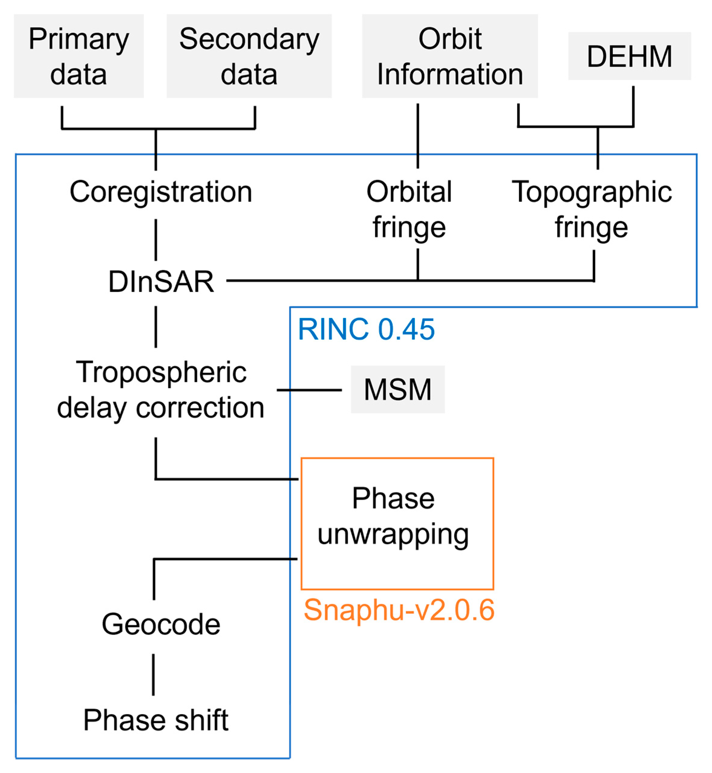
3.1. Creating Interferograms

We processed the interferograms from the L-band SAR data acquired using ALOS-2. The interferogram pairs used in this study are listed in Table 1. All SAR data used in this study were acquired in descending right-looking mode using Path 19 and Frame 2760 (Figure 3). SAR data acquired during snowy seasons are unsuitable for observing landslide dynamics because of reduced coherence (e.g., in [13,43,44]). Therefore, this study did not utilize SAR data acquired during snowy seasons. Table 1 also shows the weather conditions at the time of ALOS-2 observations. The weather conditions were observed at the JMA’s AMeDAS Otaki (Figure 3) [45]. In Table 1, the unit “h”, for instance, 0.5 h for the Primary in Pair 1, indicates that the direct solar radiation exceeded 0.12 kW/m2 at 11:00, lasting for 0.5 h. Conversely, the unit “mm”, for example, 0.5 mm for the Secondary in Pair 1, signifies that the precipitation at 11:00 was 0.5 mm.
Figure 4 illustrates the DInSAR procedure used in this study. To remove topographic fringes and geocode interferograms, we utilized a Digital Ellipsoidal Height Model (DEHM) created from a 10 m mesh Digital Elevation Model (DEM) publicly available from the Geospatial Information Authority of Japan (GSI) [46] and the EGM96 geoid model [47]. Interferograms were multi-looked in the range direction with four looks and in the azimuth direction with five looks to match the spatial resolution of the DEM (10 m). The atmospheric noise correlated with elevation was corrected using a mesoscale model (MSM) provided by the Japan Meteorological Agency [48]. We obtained the MSM data from RISH at Kyoto University [49]. Phase unwrapping was performed using snaphu-v2.0.6 [50,51,52]. Finally, the phase was shifted to ensure that the ground movement of the reference point on GNSS positioning (Figure 1b) was set to zero. Processing until this stage was conducted using RINC 0.45 [53]. The processed interferograms were visualized on maps using ArcGIS Pro 3.1.0. In the following section, we present enlarged interferograms of the area surrounding the target landslides (coverage is shown in Figure 1b). In DInSAR, the phase of the primary data was subtracted from the phase of the secondary data. Thus, a positive displacement in the Line of Sight (LoS) indicates ground movement away from the satellite, whereas a negative displacement in the LoS indicates ground movement toward the satellite.

3.2. Accuracy Validation of Interferograms

To assess the accuracy of the interferograms generated for the landslide dynamics estimation, we compared them with the following:
(1)
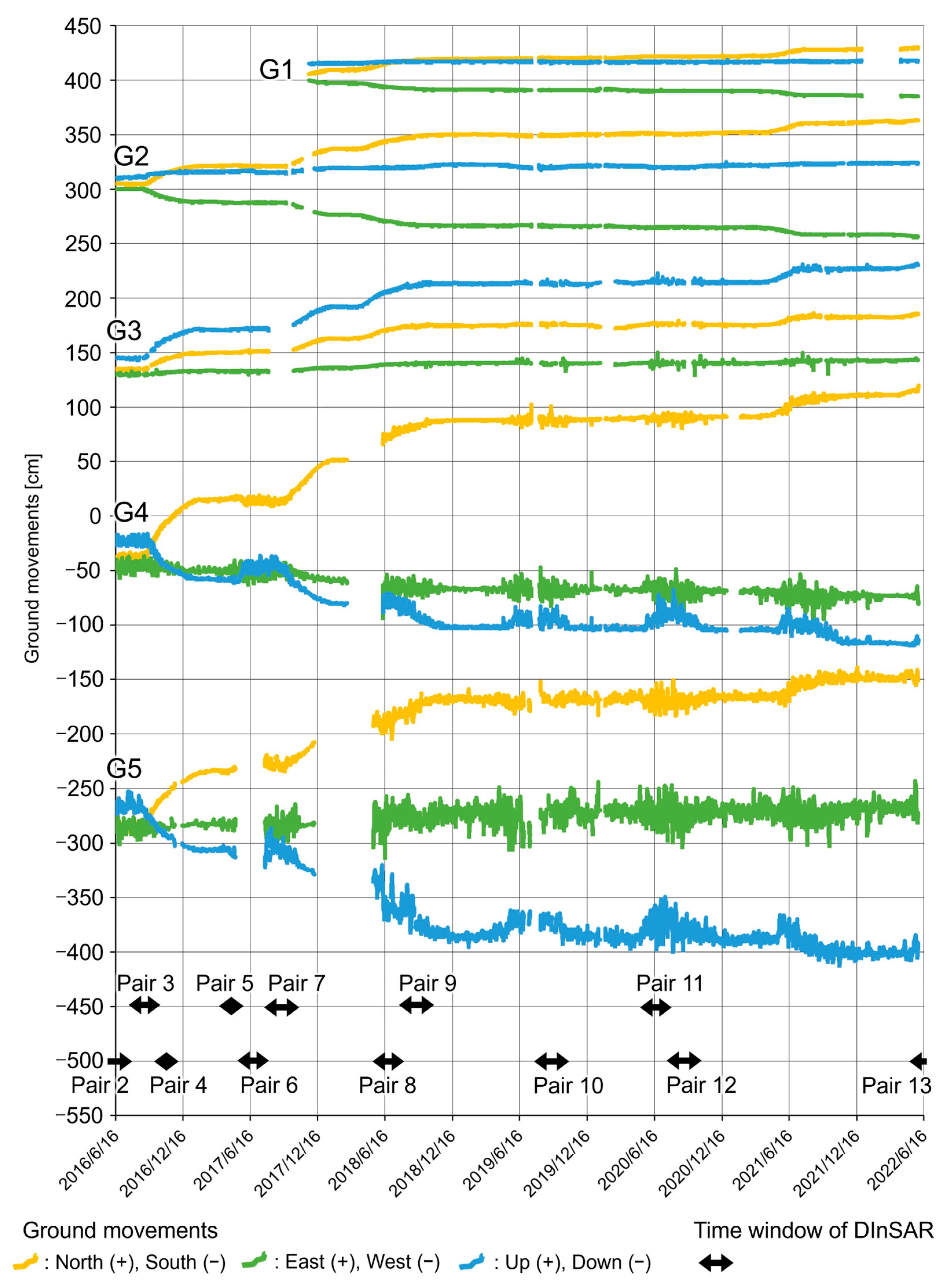
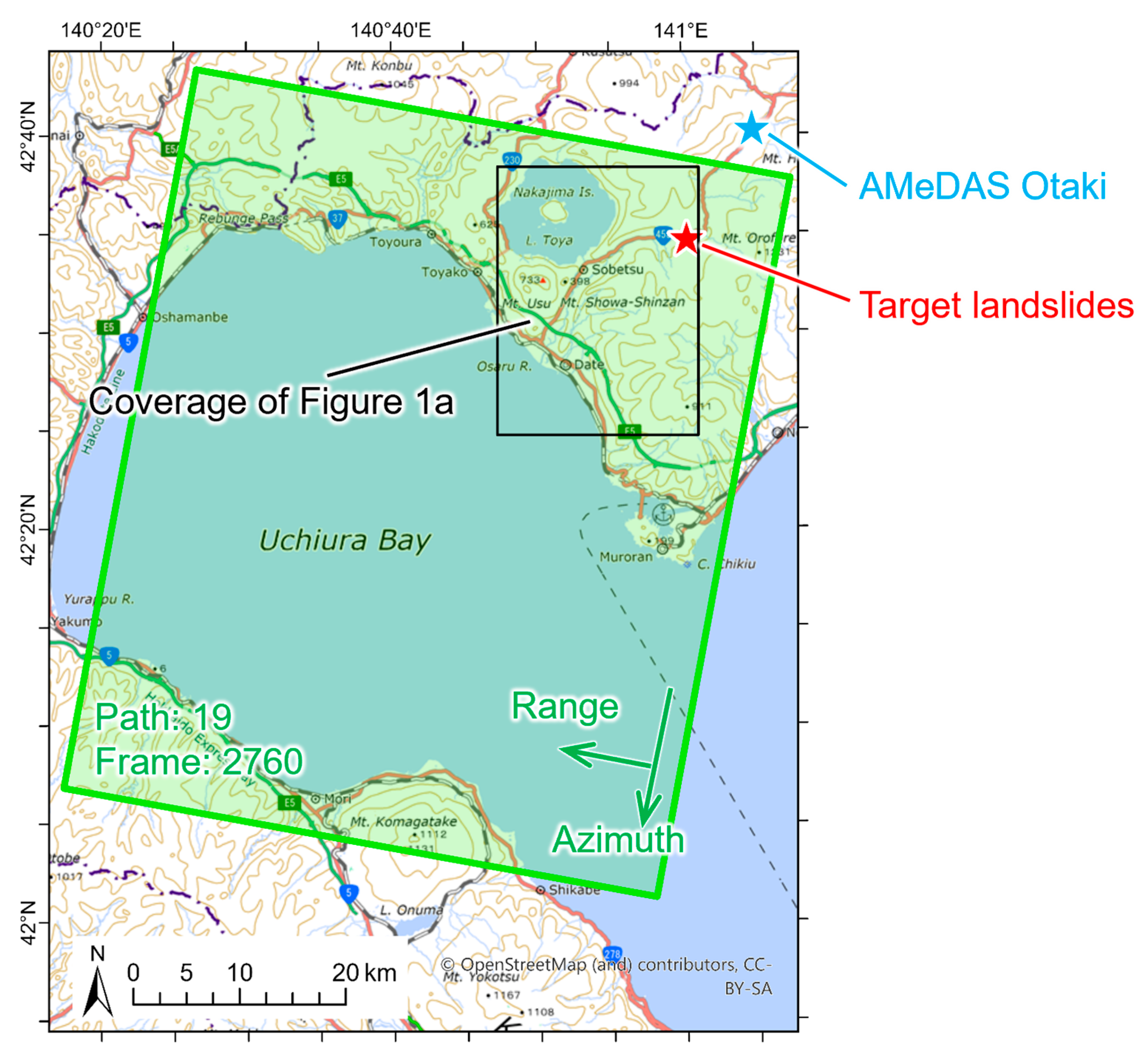
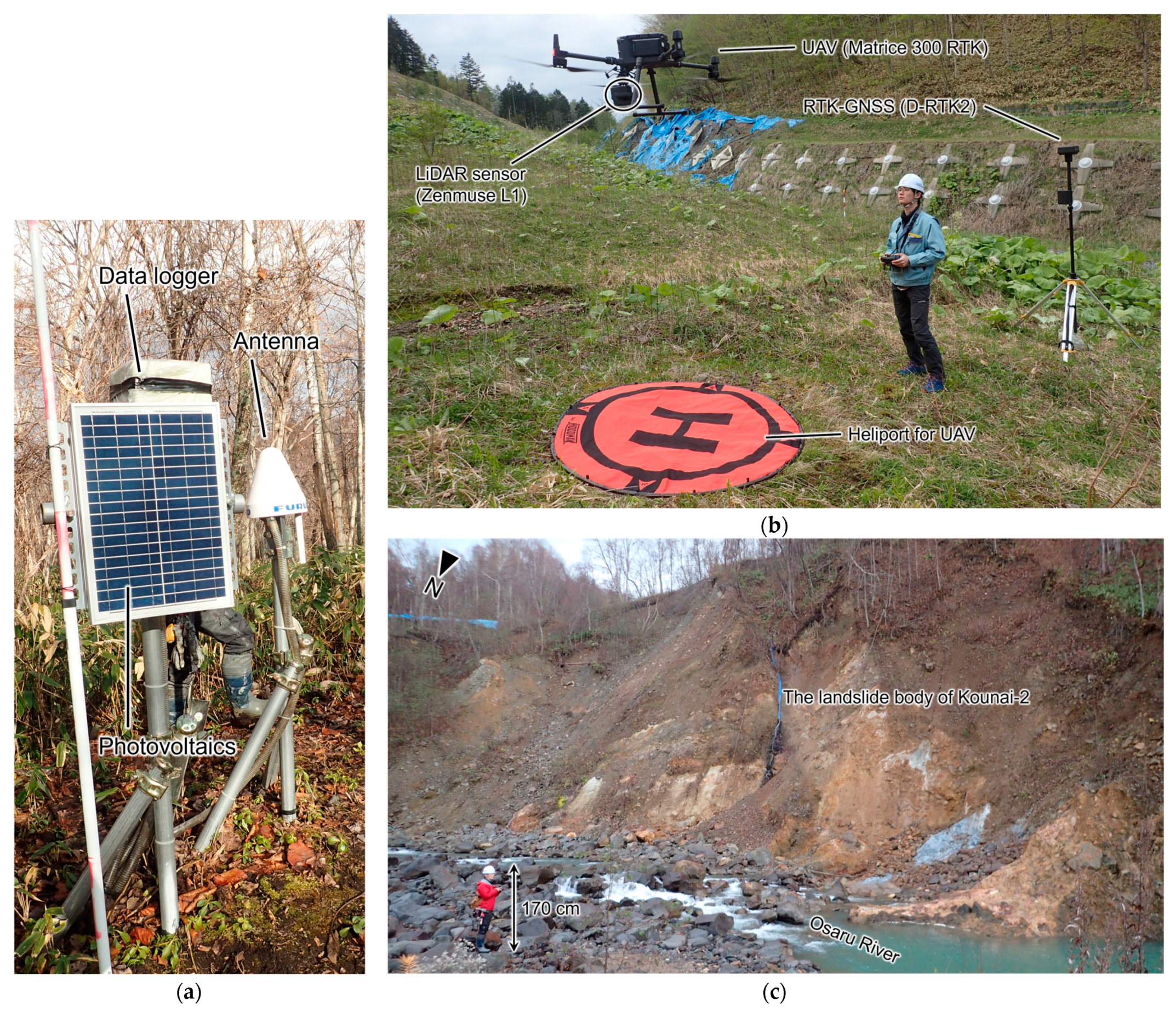
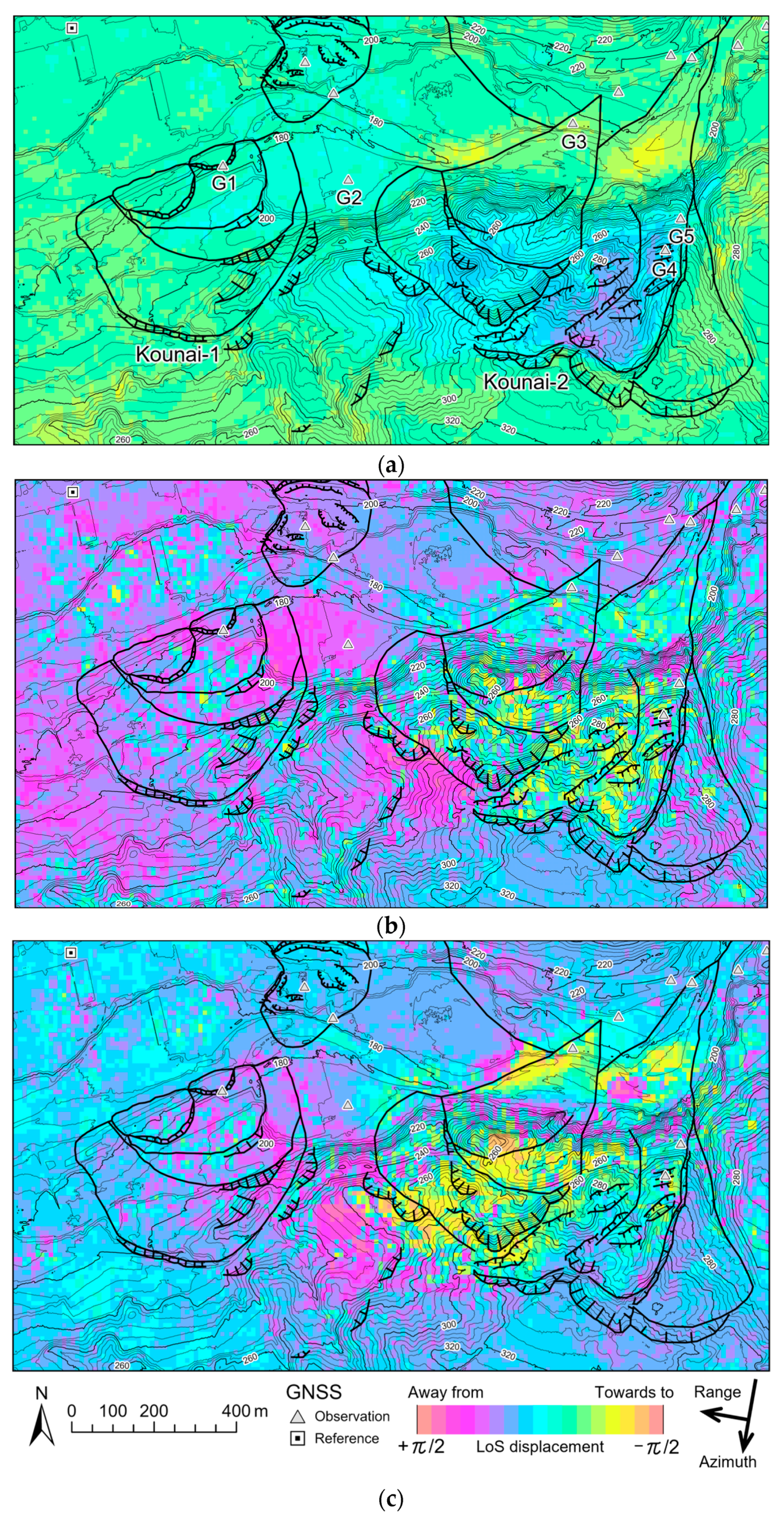
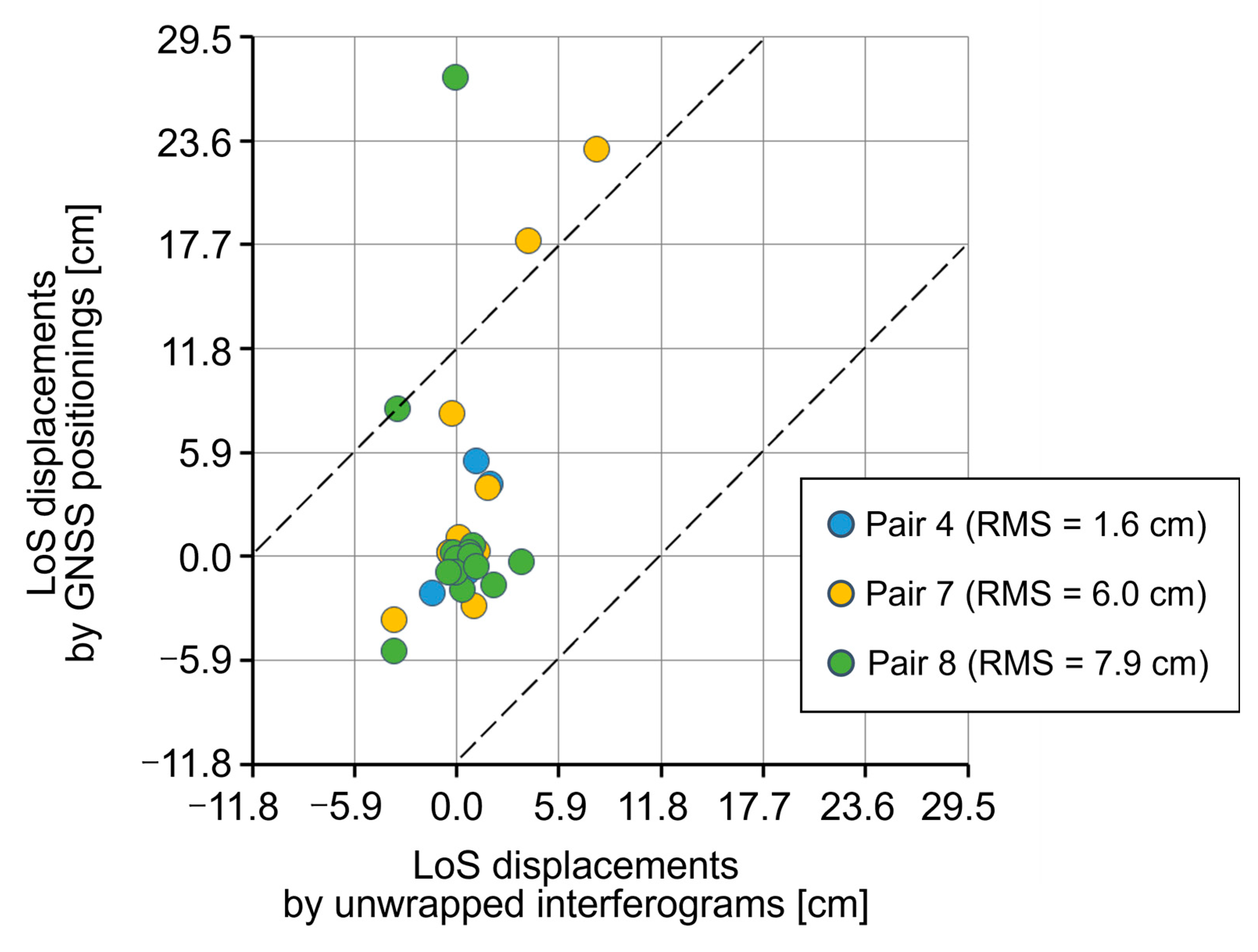
GNSS positioning (Figure 5a): We converted the ground movements observed by GNSS positioning during the same time window as the interferograms (Figure 1c) into the LoS direction based on [54] (pp. 162–163). For an incidence angle of ALOS-2 ≈ 32.5° and heading from the north of ALOS-2 (i.e., Azimuth direction) ≈ 190.5°. The locations of GNSS positioning are shown in Figure 1b. Subsequently, we calculated the residual Root Mean Square (RMS) of the GNSS-derived and DInSAR-derived LoS displacements.
(2)
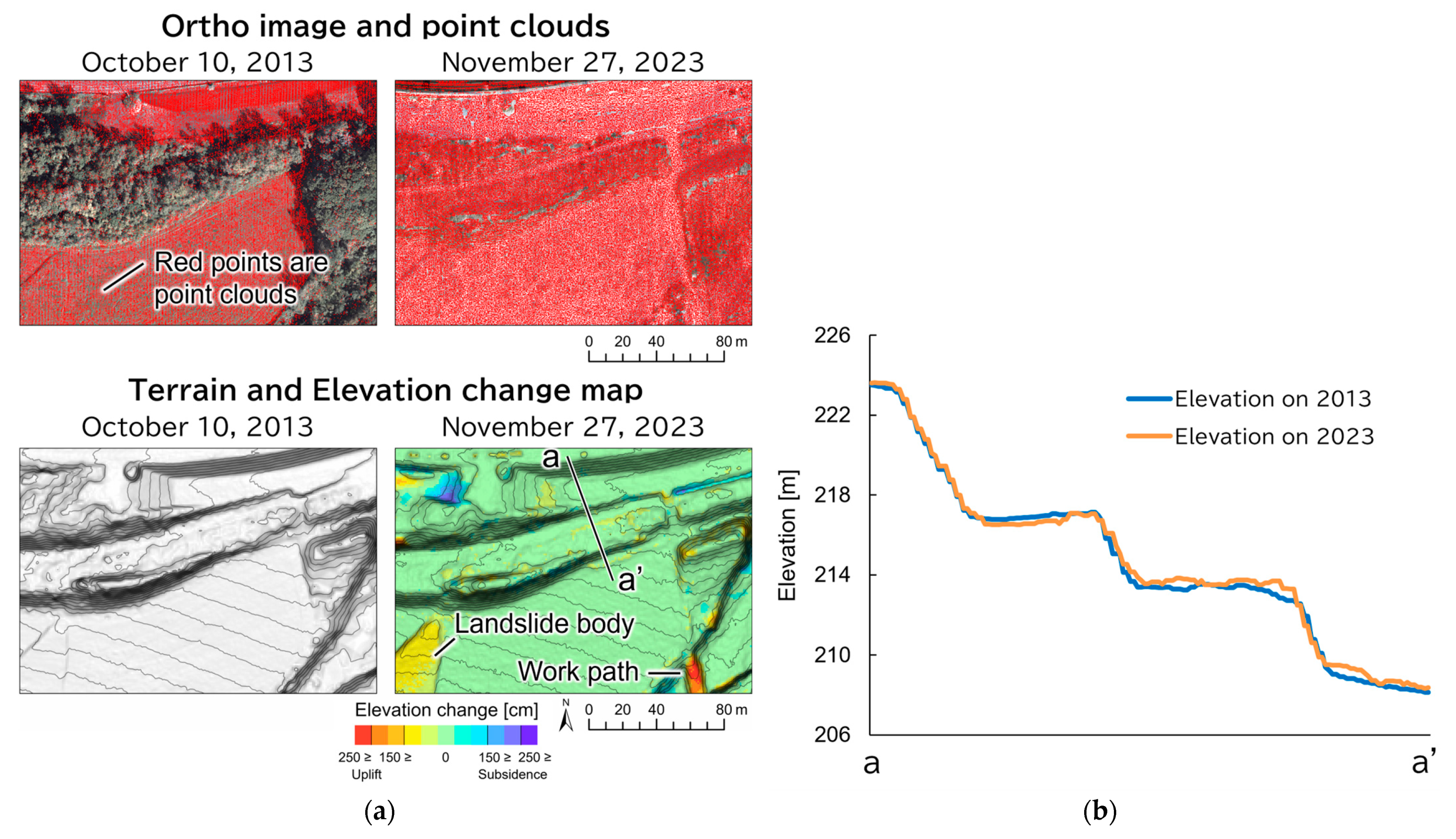
Airborne LiDAR survey (Figure 5b): Airborne LiDAR can measure elevation (e.g., see [55,56,57]). We investigated whether the areas where LoS displacement was observed in the interferograms corresponded to areas with elevation changes identified in the airborne LiDAR survey. We utilized a 1 m grid DEM generated by airborne LiDAR surveys on 10 October 2013 and 27 November 2023. The survey was planned for 10 October 2013 for the Hokkaido Regional Development Bureau and operated by the Hokkai Aerosurvey Corporation. The second project was planned and operated by the Hokkaido Research Organization. Unmanned Aerial Vehicle (UAV)-based LiDAR mapping was performed on 27 November 2023, using real-time kinematic (RTK) GNSS with a reference point. The point-cloud density during DEM creation was 4 points/m2.
(3)
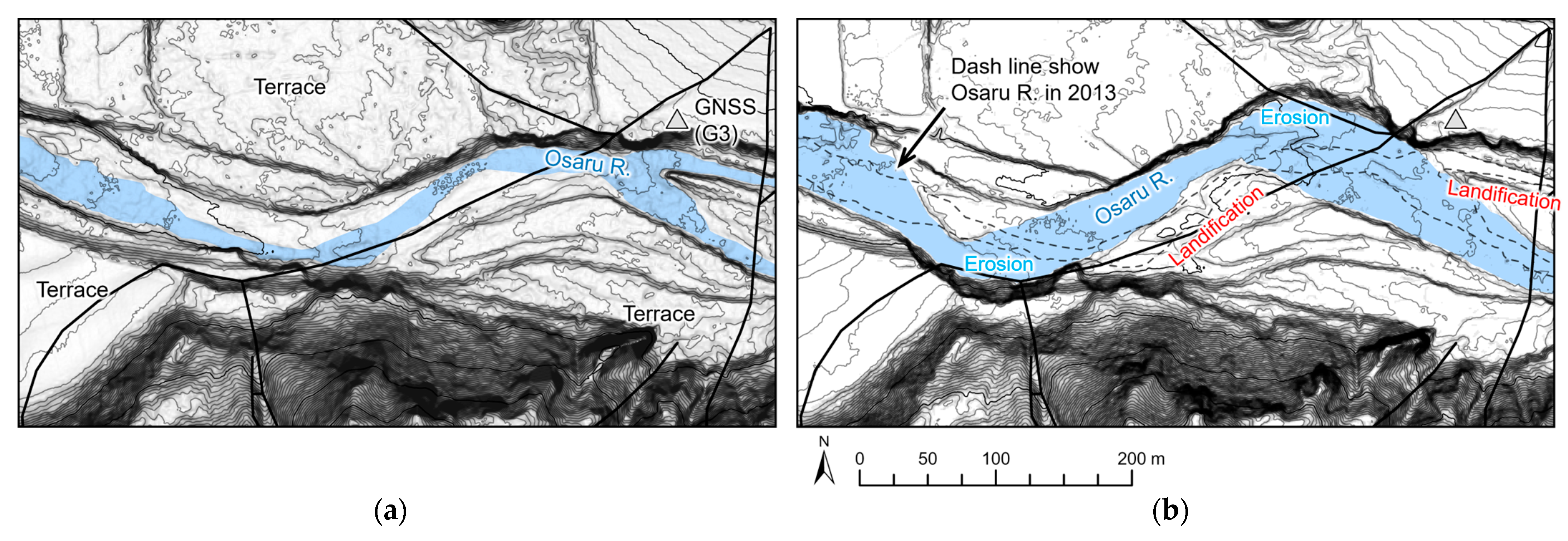
Field survey (Figure 5c): Field surveys conducted between 2022 and 2023 confirmed ground movements. We verified whether the ground movements observed during the field survey matched the LoS displacements obtained from the interferograms.
To validate the accuracy of the Airborne LiDAR survey, comparisons were conducted on both artificial and natural slopes using map-based comparison (Figure 6a) and cross-sectional profile comparison (Figure 6b). The map-based comparison revealed that the 2023 LiDAR, with degraded vegetation, had a higher point cloud density compared to the 2013 LiDAR, as shown in the orthoimage comparison (Figure 6a). However, the difference between the 1 m DEMs created from both point clouds showed almost no significant difference (Figure 6a). Similarly, the cross-sectional profile comparison indicated no substantial differences between the 1 m DEMs from both years, with a maximum elevation difference of about 1 m, likely due to the absence of vegetation, and an average variation of only about 30 cm (Figure 6b). Additionally, there were no significant discrepancies in the positions of convex landforms, and no major geometric shifts were observed in the horizontal direction (Figure 6b). Therefore, despite a maximum vertical variation of 1 m and an average variation of about 30 cm, the 1 m DEMs from both years are considered to have sufficient accuracy for detecting landslide movements.

4. Results

4.1. Comparison of Interferograms and Landslide Topography

Figure 7 shows all the wrapped interferograms created. The time windows of these interferograms and the movements observed by GNSS positioning during those periods are shown in Figure 2. As a general trend, most interferograms, with the exception of Pair 4, show phase disturbance. This might be due to the significant vegetation growth in the area, which can quickly become decorrelation. Prominent LoS displacements around Kounai-2 can be observed in Pair 3, Pair 4, Pair 7, Pair 8, and Pair 9. The periods during which these LoS displacements were observed coincide with the periods during which movements were detected by GNSS positioning (Figure 2). Furthermore, in Pair 5, a significant LoS displacement is also observed west of Kounai-2. During this period, significant movements were detected by GNSS positioning at G5, though no clear movements were observed at other observation points. However, this area also shows LoS displacement in other interferograms, such as Pair 3, Pair 4, Pair 7, Pair 8, and Pair 9 (Figure 7). Since a GNSS positioning system is not installed west of Kounai-2, verifying the nature of these phase changes using another method is necessary. Below, we focus on Pairs 4, 7, and 8, which have different time windows and periods during which movements were observed in both interferograms and GNSS positioning. Here, the time window for Pair 4 corresponds to that of ALOS-4, as well as the shortest time window of ALOS-2, while the time windows for Pair 7 and Pair 8 correspond to the typical time windows of ALOS-2 (Table 1).
Figure 8 shows the wrapped interferograms (Pairs 4, 7, and 8 in Table 1), where the LoS displacements indicative of the target landslide dynamics were observed. Figure 9 shows the unwrapped interferograms of the same interferograms in Figure 8. Table 2 lists the ground movements observed by GNSS positioning during the same period, as shown in Figure 8 and Figure 9. The “No data” in Table 2 shows periods during which GNSS positioning systems were not operated. Figure 8 and Figure 9 show notable LoS displacements around the target landslides. From Figure 8, it is apparent that the LoS displacements within the target landslides are not uniform. Below, we explain the LoS displacements observed for each interferogram.
In Pair 4 (Figure 8a and Figure 9a), notable LoS displacements were observed around Kounai-2. At the toe of Kounai-2, LoS displacements were observed to move toward the satellite. These displacements cover the left basin of the Osaru River. At the main landslide body of Kounai-2, the LoS displacements moving away from the satellite were observed. The largest LoS displacement (3.5 cm from the satellite) was observed directly beneath the main cliff at Kounai-2. These displacements extend toward the west, where similar LoS displacements are observed in parts of Kounai-1. During Pair 4, the LoS displacements observed by GNSS positioning were as follows: −0.9 cm at G2, −2.1 cm at G3, 4.1 cm at G4, and 5.4 cm at G5 (Table 2). G1 was not operated.
In Pair 7 (Figure 8b and Figure 9b), LoS displacements in the direction moving toward the satellite were observed at the toe of Kounai-2 and some parts directly beneath the main cliff. On the west side of Kounai-2, LoS displacements moving away from the satellite were also observed, although they were not as notable as those in Pair 4. During Pair 7, the LoS displacements observed by GNSS positioning were as follows: −2.8 cm, −3.6 cm, 17.9 cm, and 23.1 cm at G2, G3, G4, and GR, respectively (Table 2). G1 was not operated.
In Pair 8 (Figure 8c and Figure 9c), LoS displacements moving toward the satellite were observed in the eastern half of Kounai-2, whereas, in the western half of Kounai-2, LoS displacements away from the satellite were observed. These displacements extend further to the west and connect with Kounai-1. However, the LoS displacements in Kounai-1 are less notable than those in Kounai-2. Interestingly, notable LoS displacements were observed between both landslides. At the Kounai-2 toe, LoS displacements moving toward the satellite were observed. During the period covered by Pair 8, the LoS changes observed by GNSS positioning were as follows: −1.6 cm at G1, −1.9 cm at G2, −5.4 cm at G3, 8.4 cm at G4, and 27.2 cm at G5 (Table 2).

4.2. Comparison of Interferograms and GNSS Positioning

We calculated the residuals of the ground movements between the GNSS positioning (Figure 1b) and unwrapped interferograms of Pairs 4, 7, and 8 (Figure 9), as shown in Figure 10. However, five GNSS positioning systems did not operate on Pair 4, two GNSS positioning systems did not operate on Pair 7, and one GNSS positioning system did not operate on Pair 8. These GNSS positioning systems are not in operation because the 17 GNSS positioning systems were not installed all at once but were installed in stages over several years. In Figure 10, the dashed lines represent the residuals within a range of 11.8 cm, which is half the wavelength of ALOS-2. Out of the 40 plotted points, only the following four points exceed the 11.8 cm of residuals. In G4 of Pair 7, 17.9 cm moved away from the satellite on GNSS positioning, 4.1 cm moved away from the satellite on interferogram, and the residual was 13.8 cm (Table 2). In G5 of Pair 7, 23.1 cm moved away from the satellite on GNSS positioning, 8.1 cm moved toward the satellite on interferogram, and the residual was 15.0 cm (Table 2). In G4 of Pair 8, 8.4 cm moved away from the satellite on GNSS positioning, 3.4 cm moved toward the satellite on interferogram, and the residual was 11.8 cm (Table 2). In G5 of Pair 8, 27.2 cm moved away from the satellite on GNSS positioning, 0.1 cm moved toward the satellite on interferogram, and the residual was 27.3 cm (Table 2). The RMS values of all residuals were 1.6 cm for Pair 4, 6.0 cm for Pair 7, and 7.9 cm for Pair 8 (Figure 10).

4.3. Comparison of Interferograms and Airborne LiDAR Survey

Figure 11 shows the elevation changes from 10 October 2013 to 27 November 2023, at the target landslides. At the head of Kounai-2 (“A” in Figure 11), notable subsidence ranging from 120 to 370 cm is observed. Pair 4 of the interferograms (Figure 8a and Figure 9a) shows harmonious LoS displacement alongside the observed elevation change in this area. However, in Pairs 9 and 10 of the interferograms (Figure 8b,c and Figure 9b,c), LoS displacements moving toward the satellite were observed, and they were not in harmony with the elevation change (Figure 11). At the toe of the Kounai-2 (“B” of Figure 11), an uplift ranging from 120 to 300 cm is observed. In this area, harmonious LoS displacements moving toward the satellite were observed in Pairs 4, 7, and 8 (Figure 8 and Figure 9), along with the elevation change (Figure 11). Notable subsidence was observed on the western side toe of the Kounai-2 (“C” in Figure 11). Comparing the Digital Terrain Model (DTM) between 10 October 2013 (Figure 12a) and 27 November 2023 (Figure 12b) near “C” in Figure 11, it is evident that the riverbank has undergone substantial erosion. Therefore, this change in elevation was attributed to riverbank erosion by the Osaru River.
Notable elevation changes compared to Kounai-2 were not observed in Kounai-1 (Figure 11). The elevation increase observed at the toe of Kounai-1 (“D” in Figure 11) is attributed to riverbank protection works. The unwrapped interferograms show LoS displacements moving away from the satellite, which are particularly pronounced in Pairs 4 (Figure 9a) and 8 (Figure 9c).
In the eastern area between the Kounai-1 and Kounai-2, specifically at G2 in Figure 1c (“E” in Figure 11), an uplift ranging from 70 to 190 cm was observed. In the unwrapped interferograms, ground movement away from the satellite was observed for Pair 4. However, ground movements toward the satellite were observed in Pairs 7 and 8. On the western side of Kounai-2’s main cliff (“F” in Figure 11), a linear subsidence of 120 to 370 cm was observed. This subsidence area is contiguous with the main cliff of Kounai-2 (Figure 11). Around this subsidence area, ground movement away from the satellite was observed in the interferograms (Figure 9).

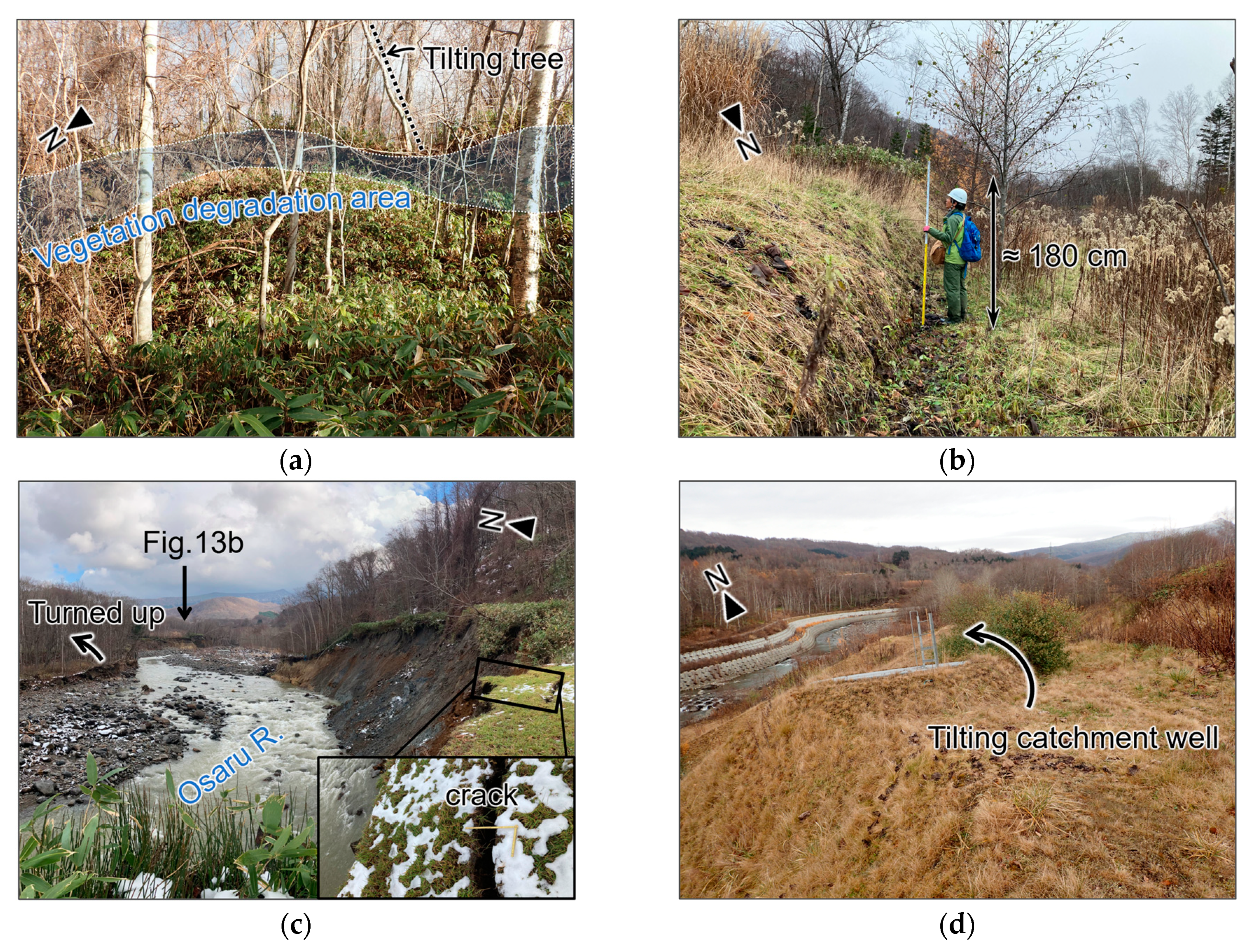
4.4. Comparison of Interferograms and Field Survey

We conducted field surveys at the elevation change locations (“A” to “F” in Figure 11). Figure 13 shows a photograph of the ground movements captured during the field surveys. The shooting points of Figure 13a–f correspond to “A” to “F” in Figure 11.
  • Around Kounai-2, where subsidence of approximately 120 to 370 cm was observed by aerial LiDAR survey (“A” in Figure 11), some cliffs several meters high were observed, with vegetation stripped off and trees tilting to the slope side (Figure 13a).
  • At the toe of Kounai-2, where the flat surface of the river terrace was uplifted, an aerial LiDAR survey (“B” in Figure 11) observed a cliff of approximately 180 cm (Figure 13b), forming a range from approximately 120 to 300 cm.
  • On the western side of Kounai-2, where the effects of river erosion were observed (“C” in Figure 10 and Figure 12), cracks formed on the attacking slope side of the Osaru River (Figure 13c). Additionally, the right bank of the Osaru River turned upward (Figure 13c).
  • At the toe of Kounai-1, where elevation change was observed (“D” in Figure 11), the catchment well for the landslide was tilted northward (Figure 13d).
  • At the area between Kounai-1 and Kounai-2, where an uplift from approximately 70 to 190 cm was observed by aerial LiDAR survey (“E” in Figure 11), the terrace was uplifted (Figure 13e).
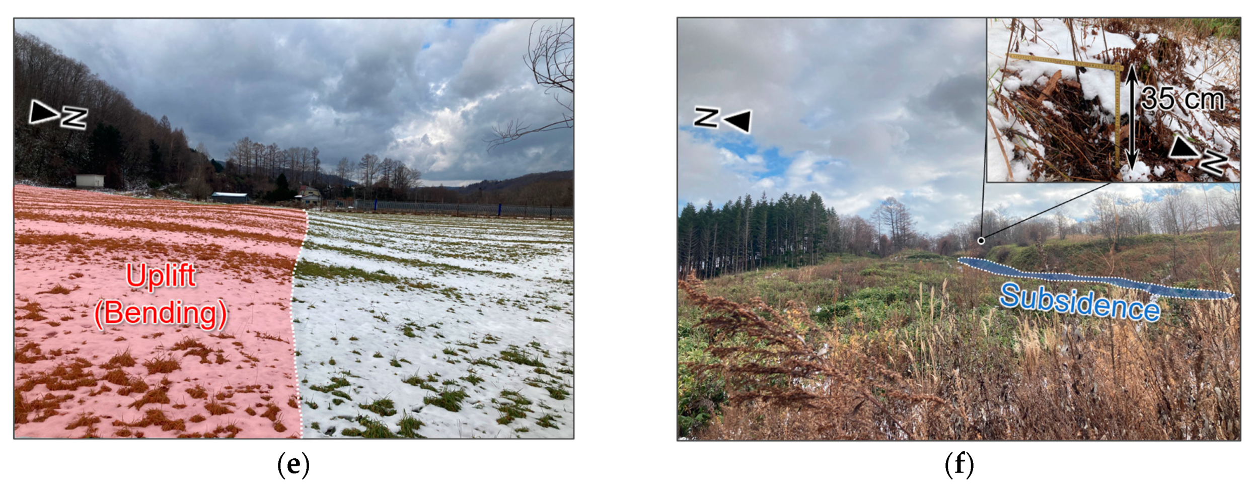
  • Near the western extension of the main cliff of Kounai-2, within the area between Kounai-1 and Kounai-2, an aerial LiDAR survey observed subsidence from about 70 to 370 cm (“F” in Figure 11). Cliffs of approximately 5 m were formed (Figure 13f), and at the location where this cliff climbed, a fresh small cliff of approximately 35 cm was formed (Figure 13f).

5. Discussion

5.1. Advantage of High-Temporal L-Band SAR Observations in Estimating Landslide Dynamics

The accuracy of landslide movement observations based on unwrapped interferograms with L-band SAR was confirmed at 1.51 cm compared to GNSS positioning [28]. This study also confirmed that the ground movement observation accuracy of the unwrapped interferogram for 14 days was 1.6 cm compared with GNSS positioning (Figure 10). This result confirms the results of previous studies and shows that L-band DInSAR can observe ground movements with an accuracy of approximately 2 cm. However, Pairs 7 (time window of 84 days) and 8 (time window of 70 days), which had longer time windows than Pair 4 (time window of 14 days), did not show the same observation accuracy as that of Pair 4 (Figure 10).
Kounai-2 is a particularly active landslide, and there have been reports of cycle slips occurring in interferograms when the displacement exceeds half the wavelength of SAR microwaves [34]. The wavelength of the ALOS-2/PALSAR-2 used in this study was in the L-band (23.6 cm); therefore, cycle slips occurred when the ground movement exceeded 11.8 cm. Cycle slips depend on the wavelength of the SAR microwaves; therefore, they are more likely to occur at shorter wavelengths, such as the C-band and X-band, than at the L-band [27]. Among the interferograms created in this study, residuals exceeding 11.8 cm compared to GNSS measurements were observed in G4 (residual was 13.8 cm) and G5 (residual was 15.0 cm) of Pair 7; and G4 (residual was 11.8 cm) and G5 (residual was 27.3 cm) of Pair 8 (Figure 10). It is reasonable to attribute the residuals exceeding 11.8 cm to the influence of unwrap errors caused by cycle slips. Specifically, GNSS positioning observed a 17.9 cm moving away from the satellite in G4 of Pair 7, and an unwrapped interferogram was 4.1 cm from the satellite. In this case, it was assumed that a one-cycle slip occurred, and the residuals became 2.0 cm. Similarly, G5 of Pair 7 (residual of 15.0 cm) and G4 of Pair 8 (residual of 11.8 cm) were reasonable for one-cycle slip. Two-cycle slips might have occurred in G5 of Pair 8 (residual of 27.3 cm), but a 3.7 cm residual remains. This may affect the spatial interpolation of ground movements due to the application of multiple looks to the interferograms. However, there is no doubt that cycle slip occurred because the wrapped interferogram (Figure 8c) was light blue (i.e., nonmoving) around the ground movement observed by GNSS positioning, such as G4 and G5. Therefore, it is reasonable to attribute the residuals exceeding 11.8 cm to the influence of unwrapping errors caused by cycle slips.
The landslides persisted for several months (Figure 2). This indicates that the longer the time window of the DInSAR (i.e., the more significant the ground movement), the more likely it is that a cycle slip will occur. Indeed, cycle slips occurred in the interferograms of this study with more extended time windows, such as Pair 7 (time window of 84 days) and Pair 8 (time window of 70 days), whereas no cycle slips occurred in Pair 4 with a shorter time window (time window of 14 days). In addition, the residuals between the unwrapped interferograms and GNSS positioning become smaller as the time window becomes shorter (Figure 10). This indicates that smaller time windows reveal an increased accuracy in the ground movement observed by DInSAR. For observing relatively fast landslide movements using DInSAR, as in the case of the landslides targeted in this study, phase unwrapping becomes a significant issue (e.g., Pair 7 and Pair 8). Although various methods have been proposed previously, e.g., in [58,59], a reliable method to correct unwrapping errors has not been established at this time. In other words, the only way to reduce the occurrence of unwrapping errors associated with active landslide fluctuations at this time is to increase the temporal resolution of SAR to suppress the occurrence of cycle slips. Specifically, since many unwrapping methods assume that the phase difference between two adjacent pixels does not exceed 2π [58], high-frequency observations with longer-wavelength SAR are effective in suppressing the occurrence of cycle slips. Therefore, high-temporal observation with L-band SAR, whose wavelength is longer than that of C- and X-band SAR, enables DInSAR with a short time window, which allows for highly accurate observation of active landslides that are difficult to observe with conventional DInSAR methods.

5.2. Dynamics of Kounai-1 and Kounai-2

Initially, the sliding areas of Kounai-1 and Kounai-2 were estimated. DInSAR and other surveys have observed ground movements that approximately fit the landslide terrain of a previous study [33] (e.g., Figure 9 and Figure 11). However, some ground movements, such as the area between Kounai-1 and Kounai-2, show locations that deviate from conventional assumptions. This indicates that the extent of movement in Kounai-1 and Kounai-2 was broader than previously assumed. Therefore, redefining the sliding area of the target landslide was necessary.
We noticed that the phase of the interferograms was reversed on the western side of Kounai-2 (Figure 8 and Figure 9). Phase reversal shows the boundaries of the moving and stable areas. This is further supported by the aerial laser survey (“F” in Figure 11) and field survey (Figure 13f), which show the boundaries of moving and stable areas in this location. Moreover, according to the interferograms (Figure 8 and Figure 9), the LoS displacement observed at this location connected Kounai-2 to Kounai-1 along a small valley. Therefore, we considered this location to be the head of the landslide shared by Kounai-1 and Kounai-2. In other words, Kounai-1 and Kounai-2 are subunits of the same large-scale landslide.
Based on these considerations and the topographic interpretation, we propose a new classification diagram of the target landslide (Figure 14) and define the large-scale landslide, including Kounai-1 and Kounai-2, as a “Kounai landslide.” This new definition of the Kounai landslide is consistent with the interferogram (Figure 14a) and aerial laser survey (Figure 14b). Defining the Kounai landslide can explain why the horizontal direction and timing of the ground movement observed in the GNSS positioning remain consistent, even at Kounai-1 and Kounai-2 (Figure 1c and Figure 2). The GNSS’s harmonic movement indicates the Kounai landslide movement, which we have been trying to understand by focusing on its subunits. Understanding that Kounai-1 and Kounai-2 are subunits of the Kounai landslide provides crucial information for devising countermeasures. Without adequate planning of countermeasures for the Kounai landslide, there would be no essential solution for the disaster. This definition of the landslide area is possible only because of spatial dynamic analysis by remote sensing, as undertaken in this study.
Next, we estimated the directions of movement of Kounai-1 and Kounai-2. Because the GNSS positioning showed northward or northwestward movement, the Kounai landslide moved northward or northwestward (Figure 1c). This is consistent with the LoS displacements in the interferograms (Figure 14a). However, the aerial LiDAR survey showed a notable elevational change around Kounai-2, whereas no elevational change was observed around Kounai-1 (Figure 14b). While the interferograms show a composite vector of horizontal and vertical movements, the aerial laser survey shows only vertical movement. Therefore, it is considered that Kounai-1 moves nearly horizontally, whereas Kounai-2 moves both vertically and horizontally. Our estimated dynamics are consistent with the results of the field survey. The northward tilting of the catchment well at the end of Kounai-1 (Figure 13e) can be explained by the stress imposed by Kounai-1 from the south. Conversely, if Kounai-1 moved vertically, pushing the catchment well up from the bottom, the catchment would tilt south. In addition, at the toe of Kounai-2, the terrace was uplifted to form a near-vertical cliff (Figure 13b) because Kounai-2 pushed the terrace up from the bottom. If Kounai-2 moved horizontally, the toe ridge would be more rounded.
These differences in landslide dynamics might have occurred because of river erosion and geological conditions (e.g., rock composition). River erosion can render slopes gravitationally unstable, thereby promoting landslide activity (e.g., see [60,61,62]). Rocks have different densities depending on their type [63]. The higher the density of rocks with a composition slope, the more susceptible the slope was to gravitational deformation. We considered the dynamics of Kounai-1 and Kounai-2 based on these factors. Kounai-1 is mainly composed of terrace deposits (Figure 1b). In contrast, Kounai-2 is composed of andesite (Figure 1c), with a higher specific gravity than terrace deposits. In addition, the course of the Osaru River is straight and protected by banks, making it less susceptible to erosion around Kounai-1. In contrast, the Osaru River meandered, and its banks eroded around Kounai-2 (Figure 11 and Figure 12). Therefore, compared with Kounai-1, Kounai-2 has more gravitational instability factors. These factors may have affected the dynamics of Kounai-1 and Kounai-2. However, to clarify these effects on landslide dynamics, it is necessary to investigate the geological structure (i.e., the shape of the sliding surface) and spatiotemporal changes in river erosion.

6. Conclusions

In this study, we applied L-band DInSAR to two active landslides (Kounai-1 and Kounai-2) and attempted to understand their dynamics using interferograms with various time windows. As a result, we could more accurately and spatially understand the dynamics of these landslides using interferograms with a 14-day time window than those with 70-day and 84-day time windows. This implies that the 14-day L-band SAR observations suppressed the occurrence of cycle slips in active landslides. In addition, we revealed that the target landslides were subunits of a large-scale landslide (the Kounai landslide) and exhibited different dynamics for each subunit based on the 14-day interferogram and other results. This is the first time that the previously unclear dynamics of the target landslides have been clarified based on objective and quantitative observational data.
These results reveal that high-temporal L-band SAR observations, which are expected to be realized in the near future (e.g., ALOS-4, NISAR, and ROSE-L), can enable an understanding of the dynamics of relatively fast-moving active landslides, as such an understanding has been difficult to gain with conventional long-time window DInSAR, and provide valuable information for landslide disaster mitigation. However, there are still unresolved issues, including a quantitative assessment of how geological conditions and erosion of the Osarugawa River affect the dynamics of Kouchi-1 and Kouchi-2. Using high-temporal L-band SAR observations, the dynamics of landslides corresponding to river erosion observed by aerial laser survey can be determined in more detail than now. In addition, by correlating the estimated landslide dynamics with the geological conditions of each landslide unit (e.g., shape and depth of the slip surface, rock types, and metamorphism) through borehole investigations, it is possible to understand the geological factors that determined the dynamics of the landslide. We hope that high-temporal L-band SAR observations will help elucidate these landslide mechanisms and reduce future landslide disasters.

Author Contributions

S.U. conceived and designed this study; S.U. performed the DInSAR aerial UAV survey; S.U. and S.I. performed the field survey and terrain interpretation; S.I. performed the GNSS positioning; S.U. and T.T. managed this study. The original draft was written by S.U. and reviewed and edited by S.I. and T.T. All authors have read and agreed to the published version of the manuscript.

Funding

This study was supported by a RESTEC Research Grant in 2022, ERI JURP 2021-B-03 and 2024-B-02 at the Earthquake Research Institute, University of Tokyo, and operational expense subsidies of the Hokkaido Research Organization. Operational expense subsidies of the Hokkaido Research Organization funded the APC.

Data Availability Statement

The datasets presented in this article are not readily available because they are part of an ongoing study. Requests to access the datasets were made by the corresponding author.

Acknowledgments

This study was conducted at the 3rd Research Announcement on Earth Observations (EO-RA3), Earth Observation Research Center, JAXA. ALOS-2/PALSAR-2 SLC data are shared among the PALSAR Interferometry Consortium to Study our Evolving Land Surface (PIXEL) and provided by JAXA under a cooperative research contract with PIXEL. The PALSAR-2 data are owned by JAXA. Gentaro, Kawakami, Masazo, Takami, and Kan Fujiwara (Hokkaido Research Organisation) assisted with field surveys. Sobetsu town, Hokkaido government, Hokkaido Regional Development Breau, Ueyama-Shisui Co., Ltd., and Tokiwa Chicken Co. supported the GNSS positioning.

Conflicts of Interest

The authors declare no conflict of interest.

References

  1. Varnes, D.J. Slope movement types and process. In Landslides, Analysis and Control; Schuster, R.L., Krizek, R.J., Eds.; Special Report 176; Transportation Research Board, National Academy of Sciences: Washington, DC, USA, 1978; pp. 11–33. [Google Scholar]
  2. Ren, S.; Zhang, Y.; Li, J.; Zhou, Z.; Liu, X.; Tao, C. Deformation Behavior and Reactivation Mechanism of the Dandu Ancient Landslide Triggered by Seasonal Rainfall: A Case Study from the East Tibetan Plateau, China. Remote Sens. 2023, 15, 5538. [Google Scholar] [CrossRef]
  3. Delbridge, B.G.; Burgmann, R.; Fielding, E.; Hensley, S.; Schulz, W.H. Three-dimensional surface deformation derived from airborne interferometric UAVSAR: Application to the Slumgullion Landslide. J. Geophys. Res. Solid Earth 2016, 121, 3951–3977. [Google Scholar] [CrossRef]
  4. Raja, N.B.; Çiçek, I.; Türkoğlu, N.; Aydin, A.; Kawasaki, A. Landslide susceptibility mapping of the Sera River Basin using logistic regression model. Nat. Hazards 2017, 85, 1323–1346. [Google Scholar] [CrossRef]
  5. Sato, H.P.; Une, H. Detection of the 2015 Gorkha earthquake-induced landslide surface deformation in Kathmandu using InSAR images from PALSAR-2 data. Earth Planets Space 2015, 68, 47. [Google Scholar] [CrossRef]
  6. Dini, B.; Manconi, A.; Loew, S.; Chophel, J. The Punatsangchhu-I dam landslide illuminated by InSAR multitemporal analysis. Sci. Rep. 2020, 10, 8304. [Google Scholar] [CrossRef] [PubMed]
  7. Masumoto, M.; Nonomura, A.; Hasegawa, S.; Fujisawa, K.; Yamanokuchi, T.; Tadono, T. Estimation of slope deformation by heavy rain in July 2018 using interferometric SAR in Kagawa Pref., Japan. J. Remote Sens. Soc. Jpn. 2020, 40, 97–102, (In Japanese with English abstract). [Google Scholar] [CrossRef]
  8. Yamagishi, H. Landslides in Hokkaido; Hokkaido University Press: Sapporo, Japan, 1993. (In Japanese) [Google Scholar]
  9. Ozawa, S.; Ishimaru, S. Web-GIS based information offer of the landslide distribution data-map of Hokkaido. Rep. Geol. Surv. Hokkaido 2011, 83, 73–76. (In Japanese) [Google Scholar]
  10. Oyagi, N.; Uchiyama, S.; Ogura, M. Landslide Maps, Series 60 the central part of Kanto region explanations of landslides distribution maps. Tech. Note Natl. Res. Inst. Earth Sci. Disa. Prev. 2015, 394, 1–14. Available online: https://dil-opac.bosai.go.jp/publication/nied_tech_note/landslidemap/shared/docs/document.pdf (accessed on 6 April 2024). (In Japanese).
  11. Yagi, H. Toward practical utilization of landslide inventory map issued by NIED. In Proceedings of the Workshop on the Prediction of Landslide Disasters, Tsukuba, Japan, 3 December 2020; Yamada, R., Iida, T., Eds.; National Research Institute for Earth Science and Disaster Prevention: Ibaraki, Japan, 2021; Technical Note National Research Institute for Earth Science and Disaster Prevention 463; pp. 11–12. Available online: https://nied-repo.bousai.go.jp/records/6480 (accessed on 6 April 2024). (In Japanese)
  12. Inabe, R.; Furuta, R.; Shimizu, Y.; Inanaga, A.; Suetani, T.; Iyadomi, R. A case study of ALOS-2 emergency disaster prevention for slope failure in Sakae-mura, Simominoshi-gun, Nagano Prefecture, Japan. J. Remote Sens. Soc. Jpn. 2022, 42, 322–326. (In Japanese) [Google Scholar] [CrossRef]
  13. Takada, Y.; Motono, G. Spatiotemporal behavior of large-scale landslide at Mt. Onnebetsu-dake, Japan, detected by three L-band SAR satellites. Earth Planets Space 2020, 72, 131. [Google Scholar] [CrossRef]
  14. Liu, J.; Hu, J.; Li, Z.; Ma, Z.; Shi, J.; Xu, W.; Sun, Q. Three-Dimensional Surface Displacements of the 8 January 2022 Mw6.7 Menyuan Earthquake, China from Sentinel-1 and ALOS-2 SAR Observations. Remote Sens. 2022, 14, 1404. [Google Scholar] [CrossRef]
  15. Yang, Y.-H.; Xu, Q.; Hu, J.-C.; Wang, Y.-S.; Dong, X.-J.; Chen, Q.; Zhang, Y.-J.; Li, H.-L. Source Model and Triggered Aseismic Faulting of the 2021 Mw 7.3 Maduo Earthquake Revealed by the UAV-Lidar/Photogrammetry, InSAR, and Field Investigation. Remote Sens. 2022, 14, 5859. [Google Scholar] [CrossRef]
  16. Gao, H.; Liao, M.; Liu, X.; Xu, W.; Fang, N. Source Geometry and Causes of the 2019 Ms6.0 Changning Earthquake in Sichuan, China Based on InSAR. Remote Sens. 2022, 14, 2082. [Google Scholar] [CrossRef]
  17. Doke, R.; Kikugawa, G.; Itadera, K. Very Local Subsidence Near the Hot Spring Region in Hakone Volcano, Japan, Inferred from InSAR Time Series Analysis of ALOS/PALSAR Data. Remote Sens. 2020, 12, 2842. [Google Scholar] [CrossRef]
  18. Schaefer, L.N.; Lu, Z.; Oommen, T. Post-Eruption Deformation Processes Measured Using ALOS-1 and UAVSAR InSAR at Pacaya Volcano, Guatemala. Remote Sens. 2016, 8, 73. [Google Scholar] [CrossRef]
  19. Himematsu, Y.; Ozawa, T. Ground deformations associated with an overpressurized hydrothermal systems at Azuma volcano (Japan) revealed by InSAR data. Earth Planets Space 2024, 76, 41. [Google Scholar] [CrossRef]
  20. Aimaiti, Y.; Yamazaki, F.; Liu, W. Multi-Sensor InSAR Analysis of Progressive Land Subsidence over the Coastal City of Urayasu, Japan. Remote Sens. 2018, 10, 1304. [Google Scholar] [CrossRef]
  21. Iwahana, G.; Uchida, M.; Liu, L.; Gong, W.; Meyer, F.J.; Guritz, R.; Yamanokuchi, T.; Hinzman, L. InSAR Detection and Field Evidence for Thermokarst after a Tundra Wildfire, Using ALOS-PALSAR. Remote Sens. 2016, 8, 218. [Google Scholar] [CrossRef]
  22. Morishita, Y.; Lazecky, M.; Wright, T.J.; Weiss, J.R.; Elliott, J.R.; Hooper, A. LiCSBAS: An Open-Source InSAR Time Series Analysis Package Integrated with the LiCSAR Automated Sentinel-1 InSAR Processor. Remote Sens. 2020, 12, 424. [Google Scholar] [CrossRef]
  23. Wang, Z.; Xu, J.; Shi, X.; Wang, J.; Zhang, W.; Zhang, B. Landslide Inventory in the Downstream of the Niulanjiang River with ALOS PALSAR and Sentinel-1 Datasets. Remote Sens. 2022, 14, 2873. [Google Scholar] [CrossRef]
  24. Teshebaeva, K.; Roessner, S.; Echtler, H.; Motagh, M.; Wetzel, H.-U.; Molodbekov, B. ALOS/PALSAR InSAR Time-Series Analysis for Detecting Very Slow-Moving Landslides in Southern Kyrgyzstan. Remote Sens. 2015, 7, 8973–8994. [Google Scholar] [CrossRef]
  25. Ozawa, T.; Nohmi, H. Effect of vegetation on surface deformation measurement using InSAR investigated from laboratory experiments. J. Geod. Soc. Jpn. 2018, 64, 81–88, (In Japanese with English abstract). [Google Scholar] [CrossRef]
  26. Wei, M.; Sandwell, D.T. Decorrelation of L-band and C-band interferometry over vegetated areas in California. IEEE Trans. Geosci. Remote Sens. 2010, 48, 2942–2952. [Google Scholar] [CrossRef]
  27. Aoki, Y.; Furuya, M.; De Zan, F.; Doin, M.P.; Eineder, M.; Ohki, M.; Wright, T.J. L-band Synthetic aperture radar: Current and future applications to earth science. Earth Planets Space 2021, 73, 56. [Google Scholar] [CrossRef]
  28. Nishiguchi, T.; Tsuchiya, S.; Imaizumi, F. Detection and accuracy of landslide movement by InSAR analysis using PALSAR-2 data. Landslides 2017, 14, 1483–1490. [Google Scholar] [CrossRef]
  29. Japan Aerospace Exploration Agency. About Advanced Land Observing Satellite-4 ‘DAICHI-4’ (ALOS-4). Available online: https://global.jaxa.jp/projects/sat/alos4/ (accessed on 6 April 2024).
  30. The National Aeronautics and Space Administration. NISAR NASA-ISRO SAR MISSION. Available online: https://nisar.jpl.nasa.gov/ (accessed on 6 April 2024).
  31. European Space Agency. ROSE-L. Available online: https://sentinel.esa.int/web/sentinel/copernicus/rose-l (accessed on 6 April 2024).
  32. Morishita, Y.; Sugimoto, R.; Nakamura, R.; Tsutsumi, C.; Natsuaki, R.; Shimada, M. Nationwide urban ground deformation in Japan for 15 years detected by ALOS and Sentinel-1. Pro. Ear. Plan. Sci. 2023, 10, 66. [Google Scholar] [CrossRef]
  33. Tajika, J.; Ishimaru, S.; Kawakami, G.; Takahashi, R. Geology, landform and recent activity of the large-scale landslides in the middle basin of the Osarugawa river, Hokkaido. Rep. Geol. Surv. Hokkaido 2017, 89, 13–32. Available online: https://opac.std.cloud.iliswave.jp/iwjs0007opc/TC11110849 (accessed on 6 April 2024). (In Japanese).
  34. Usami, S. Creation and accuracy validation of a Hokkaido Active Landslide Data Map based on TS-InSAR images released by the Geospatial Authority of Japan. E-J. GEO 2024, 19, 132–144, (In Japanese with English abstract). [Google Scholar] [CrossRef]
  35. Tsunoda, F.; Agui, K.; Kurahashi, T. Analysis of landslide displacement under snow layer using interferometric SAR. In Geotechnical Engineering Magazine; Ishikawa, T., Noda, T., Eds.; The Japanese Geotechnical Society: Tokyo, Japan, 2018; Volume 66, pp. 30–31. Available online: https://thesis.ceri.go.jp/db/documents/public_detail/62664 (accessed on 6 April 2024). (In Japanese)
  36. Ota, R. 1:50,000 Geological Map of Japan, Tokushunbetsu with Explanatory Text; Geological Survey of Japan: Ibaraki, Japan, 1954; (In Japanese with English abstract); Available online: https://www.gsj.jp/Map/JP/geology4-4.html#04051 (accessed on 26 February 2024).
  37. Ota, R. 1:50,000 Geological Map of Japan, Abuta with Explanatory Text; Geological Survey of Japan: Ibaraki, Japan, 1956; (In Japanese with English abstract); Available online: https://www.gsj.jp/Map/JP/geology4-4.html#04051 (accessed on 26 February 2024).
  38. Geospatial Information Authority of Japan. Available online: https://www.gsi.go.jp/LAW/heimencho.html (accessed on 6 April 2024). (In Japanese)
  39. Wada, N.; Yahata, M.; Ohshima, H.; Yokoyama, E.; Suzuki, T. Geology and Geothermal Resources of West Iburi District, Hokkaido, Japan; Special Report 19; Geological Survey of Hokkaido: Sapporo, Hokkaido, 1988; (In Japanese with English abstract). [Google Scholar]
  40. Inokuchi, T. Landslide topography of the Sumikawa landslide. J. Jpn. Landslide Soc. 1998, 35, 11–19, (In Japanese with English abstract). [Google Scholar] [CrossRef]
  41. Matsuura, S.; Kawasaki, K.; Niimi, Y.; Asano, S.; Uchiyama, M.; Okamoto, T. A case study of investigation and mitigation measures in a caprock type of landslide in Kyushu Island, Japan. J. Jpn. Landslide Soc. 2005, 41, 522–531. [Google Scholar] [CrossRef]
  42. Watari, M. Consideration of rock slides (Ganban-jisuberi ni kansuru kousatsu). J. Jpn. Landslide Soc. 1992, 29, 1–7. (In Japanese) [Google Scholar] [CrossRef]
  43. Zhang, J.; Zhu, W.; Cheng, Y.; Li, Z. Landslide Detection in the Linzhi–Ya’an Section along the Sichuan–Tibet Railway Based on InSAR and Hot Spot Analysis Methods. Remote Sens. 2021, 13, 3566. [Google Scholar] [CrossRef]
  44. Zakharov, A.; Zakharova, L. The Bureya Landslide Recent Evolution According to Spaceborne SAR Interferometry Data. Remote Sens. 2022, 14, 5218. [Google Scholar] [CrossRef]
  45. Japan Meteological Agency. Historical Weather Data (Kako no kishou deta kensaku). Available online: https://www.data.jma.go.jp/stats/etrn/index.php (accessed on 28 June 2024). (In Japanese)
  46. Geospatial Information Authority of Japan. DEM10B. Available online: https://fgd.gsi.go.jp/download/menu.php (accessed on 8 April 2024). (In Japanese)
  47. Lemoine, F.G.; Smith, D.; Smith, R.; Kunz, L.; Pavlis, E.; Pavlis, N.; Klosko, S.; Chinn, M.; Torrence, M.; Williamson, R.; et al. Development of the NASA GSFC and NIMA Joint Geopotential Model. In Proceedings of the IAG Symposium of Gravity, Geoid, and Marine Geodesy, Tokyo, Japan, 30 September–5 October 1996; Segawa, J., Fujimoto, H., Eds.; Springer: New York, NY, USA, 1997; Volume 117, pp. 461–469. [Google Scholar] [CrossRef]
  48. Ozawa, T.; Shimizu, S. Atmospheric noise reduction in InSAR analysis using numerical weather model. J. Geod. Soc. Jpn. 2010, 56, 137–147, (In Japanese with English abstract). [Google Scholar]
  49. Research Institute for Sustainable Humanosphere (RISH), Kyoto University. RISH Data Server. Available online: http://database.rish.kyoto-u.ac.jp/index-e.html (accessed on 8 April 2024). (In Japanese).
  50. Chen, C.W.; Zebker, H.A. Network approaches to two-dimensional phase unwrapping: Intractability and two new algorithms. J. Opt. Soc. Am. 2000, 17, 401–414. [Google Scholar] [CrossRef] [PubMed]
  51. Chen, C.W.; Zebker, H.A. Two-dimensional phase unwrapping with use of statistical models for cost functions in nonlinear optimization. J. Opt. Soc. Am. 2001, 18, 338–351. [Google Scholar] [CrossRef]
  52. Chen, C.W.; Zebker, H.A. Phase unwrapping for large InSAR interferograms: Statistical segmentation and generalized network models. IEEE Trans. Geosci. Remote Sens. 2002, 40, 1709–1719. [Google Scholar] [CrossRef]
  53. Ozawa, T.; Fujita, E.; Ueda, H. Crustal deformation associated with the 2016 Kumamoto earthquake and its effect on the magma system of Aso volcano. Earth Planets Space 2016, 68, 186. [Google Scholar] [CrossRef]
  54. Hanssen, R.F. Radar interferometry: Data interpretation and error analysis. In Remote Sensing and Digital Image Processing; van der Meer, F., Ed.; Kluwer Academic Publishers: New York, NY, USA, 2001; Volume 2, pp. 162–163. [Google Scholar]
  55. Tondo, M.; Mulas, M.; Ciccarese, G.; Marcato, G.; Bossi, G.; Tonidandel, D.; Mair, V.; Corsini, A. Detecting Recent Dynamics in Large-Scale Landslides via the Digital Image Correlation of Airborne Optic and LiDAR Datasets: Test Sites in South Tyrol (Italy). Remote Sens. 2023, 15, 2971. [Google Scholar] [CrossRef]
  56. Liu, X.; Zhu, W.; Lian, X.; Xu, X. Monitoring Mining Surface Subsidence with Multi-Temporal Three-Dimensional Unmanned Aerial Vehicle Point Cloud. Remote Sens. 2023, 15, 374. [Google Scholar] [CrossRef]
  57. Hu, L.; Tomás, R.; Tang, X.; López Vinielles, J.; Herrera, G.; Li, T.; Liu, Z. Updating Active Deformation Inventory Maps in Mining Areas by Integrating InSAR and LiDAR Datasets. Remote Sens. 2023, 15, 996. [Google Scholar] [CrossRef]
  58. Molan, Y.E.; Lohman, R.B. A pattern-based strategy for InSAR phase unwrapping and application to two landslides in Colorado. J. Geophys. Res. Solid Earth 2023, 128, e2022JB025761. [Google Scholar] [CrossRef]
  59. Okuyama, S. Correction of unwrapping errors caused by Branch-cut algorithm. J. Geod. Soc. Jpn. 2010, 56, 149–155, (In Japanese with English abstract). [Google Scholar] [CrossRef]
  60. Komata, S. Sorting out landslide topography in Japan by knick line distribution, and geological signs of landslide occurrence. J. Jpn. Soc. Eng. Geol. 2015, 56, 230–238, (In Japanese with English abstract). [Google Scholar] [CrossRef]
  61. Jacobs, L.; Dewitte, O.; Poesen, J.; Maes, J.; Mertens, K.; Sekajugo, J.; Kervyn, M. Landslide characteristics and spatial distribution in the Rwenzori mountains, Uganda. J. Afr. Earth Sci. 2016, 134, 917–930. [Google Scholar] [CrossRef]
  62. Wang, F.; Xu, P.; Wang, C.; Wang, N.; Jiang, N. Application of a GIS-based slope unit method for landslide susceptibility mapping along the Longzi River, southeastern Tibetan plateau, China. Int. J. Geo-Inf. 2017, 6, 172. [Google Scholar] [CrossRef]
  63. Iwaya, T.; Kano, K. Rock densities for the geologic units in the Japanese islands: An estimate from the database PROCK (Physical Properties of Rocks of Japan). J. Geol. Soc. Jpn. 2005, 111, 434–437, (In Japanese with English abstract). [Google Scholar] [CrossRef]
Figure 1. Overview of target landslides (Kounai-1 and Kounai-2). (a) Locations of Kounai-1 and Kounai-2. (b) Geological and geomorphological conditions around Kounai-1 and Kounai-2 [33,36,37]. (c) Landslide movements were observed by GNSS positioning from 1 December 2017 to 1 June 2022. GSI map is used in Figure 1a. Landslide terrain in (b,c) is based on [33]. Geology in (b) is based on [36,37]. The maps were coordinated under JGD2011Zone11 [38].
Remotesensing 16 02687 g001
Figure 2. Landslide movement observed by GNSS positionings. Locations of GNSS positioning systems are shown in Figure 1c. The yellow line indicates north–south movement, the green line represents east–west movement, and the blue line shows vertical movement, with positive values corresponding to north, east, and upward directions, respectively. Black arrows indicate DInSAR time windows.
Remotesensing 16 02687 g002
Figure 3. The coverage of the ALOS-2 data used in this study. The GSI map was used as the base map. The maps were coordinated under JGD2011Zone11 [38].
Remotesensing 16 02687 g003
Figure 4. The flowchart of DInSAR in this study.
Remotesensing 16 02687 g004
Figure 5. The surveys were conducted to validate the accuracy of interferograms. (a) The GNSS positioning system operated in target landslides. (b) UAV-based aerial LiDAR survey. (c) Field survey of ground movements. (a) The GNSS positioning system called G4 in Figure 1c. (c) The photograph was taken at “P” in Figure 1c.
Remotesensing 16 02687 g005
Figure 6. Accuracy of the Airborne LiDAR survey. (a) Map-based comparison. (b) Cross-sectional profile comparison; cross-sectional profile line is shown in (a). The coverage of (a) is shown in Figure 1c.
Remotesensing 16 02687 g006
Figure 7. All wrapped interferograms were created in this study. Landslide terrains are based on [33]. The coverage is shown in Figure 1b. The contour is based on DEM on 10 October 2013. The maps were coordinated under JGD2011Zone11 [38].
Remotesensing 16 02687 g007
Figure 8. The wrapped interferograms were focused on in this study: (a) Pair 4 in Table 1, (b) Pair 7 in Table 1, and (c) Pair 8 in Table 1; landslide terrains are based on [33]. The coverage is shown in Figure 1b. The contour is based on DEM on 10 October 2013. The maps were coordinated under JGD2011Zone11 [38].
Remotesensing 16 02687 g008
Figure 9. The unwrapped interferograms were focused on in this study: (a) Pair 4 in Table 1, (b) Pair 7 in Table 1, and (c) Pair 8 in Table 1; landslide terrains are based on [33]. The coverage is shown in Figure 1b. The contour is based on DEM on 10 October 2013. The maps were coordinated under JGD2011Zone11 [38].
Remotesensing 16 02687 g009
Figure 10. The Relationship between the LoS displacements and the RMS of the residuals observed by the GNSS positionings and the unwrapped interferograms. The dashed lines show residuals within a range of 11.8 cm, half the wavelength of ALOS-2.
Remotesensing 16 02687 g010
Figure 11. The aerial lidar observed the elevation change. The first observation occurred on 10 October 2013, and the second was on 27 November 2023. The coverage is shown in Figure 1b. The contour is based on DEM on 10 October 2013. The maps were coordinated under JGD2011Zone11 [38].
Remotesensing 16 02687 g011
Figure 12. DTM around “C” in Figure 11: (a) DTM on October 10, 2013; and (b) DTM on 27 November 2023. The coverage is shown in Figure 11. The dashed line in (b) shows the basin of the Osaru River on 10 October 2013.
Remotesensing 16 02687 g012
Figure 13. Ground movements on field survey: (a) cliff within Kounai-2 body; (b) cliff at the toe of Kounai-2; (c) crack at Osaru River basin; (d) tilted a catchment well at the toe of Kounai-1; (e) bending of the terrace between Kounai-1 and Kounai-2; and (f) cliffs near the western side of the main cliff of Kounai-2. The locations are shown in Figure 11.
Remotesensing 16 02687 g013aRemotesensing 16 02687 g013b
Figure 14. New landslide terrain classification of the Kounai landslide: (a) compared with unwrapped interferograms of Pair 4 and (b) compared with elevation change in aerial LiDAR survey. Coverage is shown in Figure 1b. Contour is based on DEM on 27 November 2023. The maps were coordinated under JGD2011Zone11 [38].
Remotesensing 16 02687 g014
Table 1. This study used the ALOS-2 data. All data were observed in the descending orbit in the right-looking mode (Path: 19; Frame: 2760).
Pair No.Primary DateSecondary DateTime Window (Days)Primary Weather 1Secondary Weather 1
11 September 201510 November 2015700.5 h0.5 mm
224 May 20162 August 2016701.0 h0.6 h
32 August 201611 October 2016700.6 h1.0 h
411 October 201625 October 2016141.0 h1.0 h
511 April 201723 May 2017420.6 h1.0 h
623 May 20171 August 2017701.0 h0.6 h
71 August 201724 October 2017840.6 h0.7 h
822 May 201831 July 2018701.0 h1.0 h
931 July 201823 October 2018841.0 h1.0 h
1030 July 201922 October 2019840.1 h0.7 h
1119 May 202028 July 2020701.0 h0.5 mm
1228 September 202020 October 2020840.5 mmNo data 2
1317 May 202226 September 2022701.0 h0.8 h
1 The hours of sunshine on sunny or cloudy days are at 11:00 a.m.; the amount of precipitation on rainy days is at 11:00 a.m. 2 Although the data at 11:00 are missing, it is presumed not to have rained, as clear skies were observed at other times on the same day and at nearby stations.
Table 2. The GNSS positioning systems at the target landslides observed ground movements in the LoS direction. G1 to G5 show GNSS positioning systems in Figure 1c. Pair numbers are the same as those in Table 1. The unit of ground movements is centimeters.
G1G2G3G4G5
Pair No.GNSSDInSARGNSSDInSARGNSSDInSARGNSSDInSARGNSSDInSAR
4No data−0.1 1−0.90.6−2.1−1.44.11.95.41.1
7No data−0.3−2.81.0−3.6−3.617.94.123.18.1
8−1.62.1−1.90.3−5.4−3.68.4−3.427.2−0.1
1 Positive displacement is away from the satellite, and negative displacement is toward the satellite.
Disclaimer/Publisher’s Note: The statements, opinions and data contained in all publications are solely those of the individual author(s) and contributor(s) and not of MDPI and/or the editor(s). MDPI and/or the editor(s) disclaim responsibility for any injury to people or property resulting from any ideas, methods, instructions or products referred to in the content.

