Abstract
Reservoir impoundment significantly impacts the hydrogeological conditions of reservoir bank slopes, and bank slope deformation or destruction occurs frequently under cyclic impoundment conditions. Ground deformation prediction is crucial to the early warning system for slow-moving landslides. Deep learning methods have developed rapidly in recent years, but only a few studies are on combining deep learning and landslide warning. This paper proposes a slow-moving landslide displacement prediction method based on the Informer deep learning model. Firstly, the Sentinel-1 (S1) data are processed to obtain the cumulative displacement time-series image of the bank slope by the Small-BAseline Subset Interferometric Synthetic Aperture Radar (SBAS-InSAR) method. Then, combining data on rainfall, humidity, and horizontal and vertical distances of pixel points from the water table line, this study created a dataset with landslide displacement as the target feature. After that, this paper improves the Informer model to make it applicable to our dataset. This study chose the Dawanzi landslide in the Baihetan reservoir area, China, for validation. After training with 50-time series deformation data points, the model can predict the displacement results of 12-time series deformation data points using 12-time series multi-feature data, and compared with the monitoring values, its Mean Square Error (MSE) was 11.614. The results show that the multivariate dataset is better than the deformation univariate data in predicting the displacement in the large deformation zone of bank slopes, and our model has better complexity and prediction performance than other deep learning models. The prediction results show that among zones I–IV, where the Dawanzi Tunnel is located, significant deformation with the maximum deformation rate detected exceeding –100mm/year occurs in Zones I and III. In these two zones, the initiation of deformation relates to the drop in water level after water storage, with the deformation rate of Zone III exhibiting a stronger correlation with the change in water level. It is expected that deformation in Zone III will either remain slow or stop, while deformation in Zone I will continue at the same or a decreased rate. Our proposed method for slow-moving landslide displacement forecasting offers fast, intuitive, and economically feasible advantages. It can provide a feasible research idea for future deep learning and landslide warning research.
1. Introduction
The construction of large reservoirs in high and narrow valleys can significantly change the geo-hydro-mechanical conditions of the slopes around the reservoirs, thereby increasing the frequency of geological disasters, especially landslide disasters [1,2,3]. The reservoir area of Baihetan on the Jinsha River, as an essential representative of the high landslide hazard area, has seen the distribution of a large number of landslides in the area since 2021, seriously threatening the safety of the neighboring residents, infrastructures, and ecological environments [1,4]. The main problem in the research on predicting bank slope deformation in reservoirs is the lack of effective monitoring means and prediction methods. Currently, the monitoring of bank slope deformation mainly relies on ground monitoring data from the Global Navigation Satellite System (GNSS) and optical satellite images [5]. Although these data can provide helpful information, due to the limited temporal and spatial extent of these methods, they often cannot comprehensively, accurately, and intuitively reflect the deformation of reservoir bank slopes [6,7]. For GNSS, it can only provide ground deformation in one location and cannot monitor a wide range of research objectives. For optical remote sensing images, it cannot perform all-weather quantitative deformation monitoring on a landslide.
Interferometric synthetic aperture radar (InSAR) technology effectively solves the problem of monitoring and predicting the deformation of reservoir bank slopes because of the ability to perform large-scale quantitative ground deformation monitoring and a stable revisit period to form a continuous time series (e.g., the satellite revisit period of Sentinel-1 is 12 days). Over the past two decades, InSAR technology has made significant progress and has been widely applied to detecting and monitoring slow-moving landslides [8,9]. In detecting and monitoring reservoir bank slope deformation, the time-series InSAR (TS-InSAR) technique has demonstrated its ability to monitor surface deformation associated with water levels [10,11,12]. In addition, the time-series deformation and cumulative displacement maps of the TS-InSAR technique can record the spatial distribution of deformation, which is an essential help in studying the deformation process of reservoir bank slopes [13,14]. Many researchers have examined detecting and monitoring reservoir bank slope deformation using InSAR technology. For example, Li et al. [15] improved the post-processing method of long-time series InSAR results, conducted a study on the relationship between water level change and slope stability in the Xiluodu reservoir area, and derived the long-term evolution trend of the bank slopes in the reservoir area through the analyses. Dun et al. [16] used TS-InSAR to obtain deformation information on the bank slopes in the Xiangbiling section of the Baihetan Reservoir area. They combined it with Google Earth images to identify 14 potential landslide areas.
The importance of predicting ground deformation is self-evident in determining the bank slope development trend and deformation manner. Sentinel-1 (S1) SAR data provide a rich data source for the InSAR time series displacement predicting task [17]. At the same time, the deformation prediction model also has a relatively mature system after a long development period. Currently, prediction methods mainly include empirical models, semi-empirical models, numerical models, and traditional artificial neural network models [18,19,20,21]. Usually, traditional prediction methods are the deterministic calculation of future trends in slope movements or acceleration. Du et al. [22] used backpropagation neural network models to predict the displacement of active alluvial landslides in the Three Gorges reservoir area in China via rainfall-water level factors. However, the deformation mode of the reservoir bank slope is complex and diverse. These traditional prediction methods have various limitations and can only be applied to small-scale single landslides with clear deformation mechanisms. Therefore, traditional prediction methods do not apply to large-scale, complex research areas [18].
In recent years, with the rapid development of Graphics Processing Units (GPUs), deep learning models have shown great potential in natural language processing, computer vision, and time series forecasting. Many scholars have researched the InSAR displacement forecast. For example, Zhou et al. [23] proposed a new prediction process that uses gated recurrent units (GRUs) to split the InSAR deformation of landslides into trend displacement and cyclic displacement and then sum the predicted values of these two to obtain the predicted total displacement. They validated this method in the Three Gorges reservoir area and achieved good results. On the other hand, the Long Short-Term Memory (LSTM) network successfully solves the problems of gradient vanishing and explosion that may occur in traditional Recurrent Neural Networks (RNNs) when learning long-term dependencies. Studies have shown that using LSTM networks as the time series InSAR deformation forecasting model can improve prediction performance [24]. These research results show the potential of deep learning models in applying InSAR displacement forecast and provide an essential reference for future research. Of course, the prediction result obtained by the deep learning method is statistical, and there is no calculation of a physical model. Although existing studies have provided valuable experience, some issues still need to be solved. Firstly, the training data for these models are limited to InSAR time-series deformation data without considering other meteorological or hydrological data such as temperature, precipitation, and reservoir level. Second, these models’ ability to extract InSAR time series deformation features of bank slopes needs to be improved. In addition, the applicability of these models could be better for deformation mechanisms in which the change in reservoir level significantly affects deformation.
The Transformer model provides a practicable solution to the above problem. ChatGPT, the most talked about AI tool in the last two years, is based on the Transformer model [25,26]. The Transformer model has efficient parallel computation, self-attention, positional encoding, and other mechanisms that perform well in time series forecasting tasks [27]. Some researchers have attempted to combine Transformer and InSAR for deformation forecasting. For example, Wang et al. [28] used a modified Transformer model to predict the deformation generated by the freeze-thaw behavior of the permafrost around a salt lake. They discussed and evaluated the expansion trend around the salt lake based on the predicted deformation and the extracted expansion results. Their results show that the Transformer model performs well in time series forecasting tasks. Therefore, we can use the Transformer model for multi-featured bank slope deformation forecasting and deformation mechanism analysis.
Previous studies have focused on InSAR time series deformation forecasting using GRU or LSTM-based models. The InSAR time series deformation prediction method based on the Transformer model still needs to be improved in evaluating the trend of the reservoir bank slope. The Transformer model cannot output all the predicted values of a long series at once; instead, it needs to predict them one by one, which will affect the accuracy and efficiency of the prediction. Therefore, we chose the Informer [29] model with better performance in time series forecasting. Informer has better time and space complexity, which can substantially improve the efficiency of self-attention computation and model prediction. In this study, an Informer model-based InSAR time-series deformation prediction method for reservoir bank slopes is developed and combined with the SBAS-InSAR algorithm to compute and analyze deformations for long time-series for the Dawanzi reservoir area of Baihetan Reservoir. It is the first successful application of the Transformer-based network analysis method to the time series displacement prediction of bank slopes in the reservoir area. In addition, we also used the predicted deformation information combined with the water level change rule to analyze the deformation trend of the landslide. Our deformation prediction method can provide critical early warnings for the prevention and control of bank slope landslides and quantitatively assess the trend of deformers based on the predicted deformations, which is of guiding significance to the project.
2. Study Area and Datasets
2.1. Study Area
The study area lies on the southeastern edge of the Tibetan Plateau, specifically southwest of Sichuan and northeast of Yunnan. It is a middle mountainous area belonging to the lower reaches of the Jinsha River basin. The area’s topography is generally high in the northwest and low in the southeast, with great topographic relief. Moreover, the gullies here are developed, crisscrossed, and deeply cut, most of which are in the shape of a “V”. The Jinsha River bounds the trend of the main gorges and mountains, with the left bank orientated in a nearly north–south direction and the right bank orientated in a north–east direction. The elevation of the top of the left bank is generally around 2000 m, and the relative height difference of the terrain is about 1400 m; the elevation of the top of the right bank is generally between 2500~3000 m, and the elevation of the top of a few mountains reaches more than 3000 m. The relative height difference of the terrain reaches about 2000 m. In general, slope landform and weathering erosion types dominate the area from Heishui River to Aizigou. The road elevation of the study area is 903–916 m, located in Qiluogou Township, Ningnan County. The northern end (downstream) outlet is about 22 km away from the dam site of Baihetan Hydropower Station (Figure 1b). The regional faults developed around the study area mainly include the Daliangshan fault zone, the Zemuhe fault zone, the Xiaojiang fault zone, etc. The most close regional fault is the Daliangshan fault zone [1,30,31]. According to the geological conditions, structural conditions and macroscopic deformation characteristics of the bank slope along the Dawanzi Tunnel, the bank slope is divided into I, II, III and IV zones, a total of 4 sections, as shown in Figure 1c.
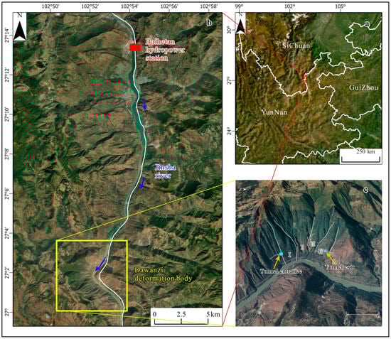
Figure 1.
Location of the study area. (a) The approximate location of the study area. It lies at the junction of Sichuan Province and Yunnan Province in China. (b) The relationship between the study area and the Baihetan Hydropower Station and the Jinsha River, where the white strip is the Jinsha River, and the yellow box is the coverage of the SAR image. (c) Engineering geological zoning.
The study area lies within the subtropical monsoon climate zone, where distinct dry and wet seasons occur throughout the year. The dry season is from November to April next year, and the rainfall is scarce. The wet season is from May to October, and the precipitation is abundant, accounting for more than 80% of the annual precipitation. The warm and dry climate has an average annual temperature of 15~21°C. Jinsha River Valley is a famous dry-hot valley. The climate has obvious zonality in the vertical direction. With the increase in altitude, the temperature decreases and the precipitation increases [32].
The rock formation in the study area is composed of the middle-thick dolomite of the lower Cambrian (), the thin sandstone of the middle Xiwangmiao Formation () and the dolomite of the upper Erdaoshui Formation (), overlying the Quaternary (). Engineering geological mapping and drilling have revealed that the overlying strata consist of colluvial deposits () and slip deposits (). The bedrock is the Middle Cambrian Xiwangmiao Formation () and the Upper Cambrian Erdaoshui Formation () [1].
2.2. Datasets
2.2.1. SAR Datasets
We acquired SAR data from the Sentinel series of SAR satellites launched by the European Space Agency in 2014. It is C-band (wavelength ~5.6 cm [33]) SAR data, known for its high sensitivity to small deformations. In this study, we collected 86 scenes of S1A SAR data with VV polarization from 3 January 2021 to 29 December 2023 to obtain the historical deformation of deformers in the Dawanzi landslide and predict its deformation trends. Unfortunately, no SAR data are available for June 2023-July 2023 in this region. The satellite has a revisit period of 12 days in the region with a line-of-sight incidence angle of around 42°. Before multilooks processing, its resolution in the radar coordinate system is 2.33m in range direction and 13.97m in azimuth direction. The multilooks coefficients are 10 and 2, respectively. After multilooks processing, we achieved a range resolution of 23.29 m and an azimuth resolution of 27.94 m. Because the deformation area mainly lies on the left bank of the Jinsha River. The descending track data have severe shadows and layovers in the target area. Therefore, this study utilizes the ascending SAR data, which offers better performance.
2.2.2. Other Datasets
The hydrological monitoring station stands at the Baihetan hydropower station. It records the water level and precipitation at 8:00 a.m. every day. The water level accuracy is at a centimeter level, and the rainfall accuracy is at 0.1 mm. This study used data from January 2021 to January 2024. Since the water storage in April 2021, the water level changed from 650 m to fluctuate from a low water level of 775 m to a high water level of 825 m (Figure 2), which significantly impacts the stability of the reservoir bank slopes.
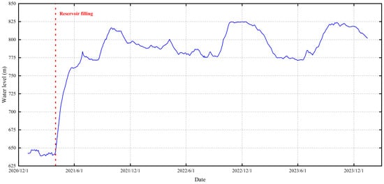
Figure 2.
Water level changes in the study area from January 2021 to January 2024.
We obtained the Digital Elevation Model (DEM) using a UAV DJI M300 RTK combined with a Zen L2 lens, and we conducted the UAV flight in October 2023. The L2 lens equipped with Light Detection And Ranging (LiDAR) emits a 905 nm electromagnetic wave, effectively penetrating the vegetation. The DEM created can better extract the proper elevation of the study area.
This study also used the fifth-generation European Centre for Medium-Range Weather Forecasts (ECMWF) reanalysis data (ERA5) [34] distributed on a 0.25° × 0.25° grid daily 2-m dew point temperature data, which is another manifestation of soil moisture.
Moderate-resolution Imaging Spectroradiometer (MODIS) is a large-scale space remote sensing instrument developed by NASA to understand global climate changes and human activities’ impact on climate [35,36]. This study used the normalized difference vegetation index (NDVI) data of the MODIS from January 2021 to January 2024. The time resolution of the data was 16 days, and the spatial resolution was 250 m × 250 m. We perform linear interpolation sampling on the corresponding date to obtain NDVI data corresponding to the same InSAR date.
3. Methodology
Figure 3 illustrates the workflow. In this study, we first preprocess the various features required for a forecast related to deformation. Subsequently, we utilized 86 scenes of S1 data and a Systeme Probatoire d’Observation de la Terre (SPOT) DEM with a resolution of 6m for SBAS processing, resulting in 86 cumulative deformation images with a reference date of 3 January 2021. The time and deformation characteristics were obtained by cropping, grid turning point, grid sampling and other operations in ArcGIS Pro 3.0. The deformation feature is the target feature in this multivariate prediction univariate task.
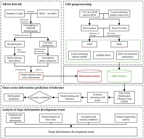
Figure 3.
The workflow of bank slope deformation forecasting based on Informer.
We extract the corresponding elevation information for each pixel using the precise DEM generated by UAV with LiDAR. Then, we obtain the water level line based on the time series water level information and DEM. By subtracting the elevation information of the pixels from the water level information over the time series, we calculate the vertical drainage distance (VDD) feature. The number of VDD features is the product of the number of pixels and the time series. We calculate the nearest distance between the pixel point and the water level line over the time series using ArcGIS Pro 3.0, which yields the horizontal drainage distance feature (HDD). The number of HDD features is the same as that of VDD. NDVI and ERA5 features are acquired by sampling each pixel’s spatial position and corresponding time series. In contrast, precipitation features are sampled over the time series and applied to all pixels.
Since the initial Informer model does not apply to our dataset, we have improved the data loading part of the model. Because the deformation results of S1 data processed by the SBAS method are volatile, we use local weighted linear regression (LOESS) for time series deformation filtering so that the data can better reflect the deformation trend. Then, we use the K-means clustering method to group pixels with different deformation characteristics. After grouping, we conduct group training to obtain the most suitable model for different deformation characteristics. After verifying the model’s accuracy, we analyze the predicted results and the deformation in the whole time series and combine other factors to predict the deformation trend of the slope.
3.1. Datasets
In this paper, we use GAMMA software (https://www.gamma-rs.ch/software, accessed on 20 June 2024) to process S1A data. We use the traditional differential InSAR (D-InSAR) technology [37,38] and the technique based on improved SBAS-InSAR to calculate the cumulative deformation since 3 January 2021 [39,40,41,42].
The interferogram pairs’ perpendicular baselines are below 300 m, so all spatial baselines are short. Some studies have shown that when using two Sentinel-1 SAR images with a time difference of more than one month, the coherence of differential interferometry images significantly reduces. In order to maximize temporal coherence and promote phase unwrapping by minimizing the deformation phase, we consider the shortest time interval, so one date data can only form interferograms with the data of the following three dates at most. Figure 4 shows the spatial perpendicular baseline of the interferograms. We selected 252 pairs of interferograms with a minimum perpendicular baseline of 0.1 m and a maximum perpendicular baseline of 272.8 m. The minimum time interval was 12 days, and the maximum time interval was 96 days. The maximum time interval is due to the lack of data in S1 in the study area in June and July 2023. We use a 10 and 2 (range direction and azimuth direction) multilooks ratio to perform multilooks processing on all Sentinel-1 interferograms.
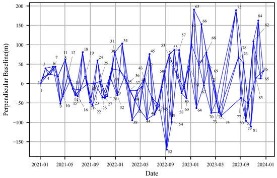
Figure 4.
Spatial perpendicular baseline of the 86 Sentinel-1 images in the SBAS-InSAR process.
For the NO. differential interferogram generated from the SAR image acquired at the moment of the slave image and the master image ( > ), the interferometric phases of the pixels with azimuthal coordinates of and distance coordinates of can be written as follows:
The first term represents the deformation phase, while the second represents the residual phase that arises due to terrain errors . The effect of this phase depends on the perpendicular baseline , the azimuth and range coordinates , and the observation angle . The third is the influence of the atmosphere. The fourth item is the phase contribution of decorrelation and other noises. Since the time baseline of this study is short, the impact of the fourth item is small.
Precise DEM and track files can remove the terrain residual phase. We use SPOT 6 m resolution DEM as the terrain reference to calculate the differential interferogram and unwrap the phase. For the atmospheric phase, unwrapping errors often occur. Regions experiencing unwrapping errors exhibit significantly higher phase standard deviation in the time series. Therefore, spatial coherence low-pass filtering and temporal coherence high-pass filtering can screen and remove the atmospheric phase. At the same time, we also use the linear de-slope method to minimize the residual tropospheric artifacts [43].
After removing the above effects, we can simplify Equation (1) as follows:
To obtain a physically meaningful settlement sequence, we express the phase in Equation (2) as the product of the average phase velocity and the time interval between two acquisition times:
The phase value of the -interferogram can be written as follows:
That is, the integral of the speed of each time period over the master and slave image time intervals. Written in matrix form as follows:
Equation (5) is a matrix with a shape of M × N. Since the SBAS-InSAR adopts a multi-master image strategy, the matrix is prone to rank deficiency. By utilizing the Singular Value Decomposition (SVD) method, we can obtain the generalized inverse matrix of the matrix , enabling us to derive the minimum norm solution of the velocity vector. Subsequently, we can obtain the deformation for each period by integrating the velocity within each period. The main results are the average deformation rate and time series deformation. The deformation obtained by InSAR technology is the direction of the radar LOS. For the convenience of comparison, projection transformation is sometimes needed. Suppose that is the azimuth angle of the satellite orbit trace, is the incident angle of the radar wave, , , and are the components of the surface deformation in the three directions of East, North and Vertical, respectively. The is the observation value of InSAR in the line of sight, then there are
Assuming that the deformation is in the vertical direction , there are
3.2. Time Series Deformation Prediction of Informer
Using the K-means clustering algorithm, we cluster different pixel groups with similar deformation characteristics based on the cumulative deformation map of the time series of a single master image. By sampling various characteristic data according to the location of the pixels, we generate time series datasets for training, verification, and prediction of the Informer model. These comprehensive datasets include time series deformation, VDD, HDD, 2 m dew point temperature, and precipitation. We then proceed with the deformation prediction with models constructed for different deformation zones.
3.2.1. Model Architecture
Figure 5 illustrates the deformation prediction model based on the Informer architecture [29].
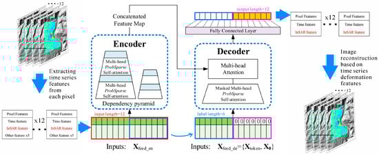
Figure 5.
Deformation forecasting model based on Informer.
On the left side of the model architecture in Figure 5, the encoder receives many long sequence inputs (green series). The ProbSparse self-attention proposed by Informer replaces the normative self-attention. The blue trapezoid is a self-attention distillation operation used to extract the dominant attention and significantly reduce the network size. Layer-stacked replicas improve the robustness of the model. On the right side is the decoder. The decoder receives long sequence input, fills the target element to zero, measures the feature map’s weighted attention composition, and generatively predicts the output element (orange series).
3.2.2. Efficient Mechanism in Model
Informer addresses three issues found in classical Transformer models: Firstly, it reduces the high complexity of self-attention calculation. Secondly, it mitigates the high complexity associated with Encoder stacking. Thirdly, it improves the slow prediction speed. Specifically, the Informer employs ProbSparse Self-attention and Self-attention Distilling in the Encoder and introduces the Start token in the Decoder.
We use the time series deformation of each pixel in the InSAR deformation image as the target feature for the multivariable prediction univariate task. Additionally, we use the other features of the pixel as the input dataset. Throughout the training process, the model progressively learns the weight matrix. Subsequently, it assigns this matrix based on the training weight of the fully connected layer to derive the query vectors Q, the key vector K, and the value vector V.
The definition of the self-attention mechanism of the specification is rooted in queries vectors Q, keys vectors K and values vectors V [26]. , where , , and is the input dimension. According to Tsai [44], the attention of the i-th query is defined as a kernel smoother in the probability form:
Tsai also highlighted that attention calculation requires secondary dot product calculation, leading to memory usage reaching , where represents the number of queries and vectors and represents the number of key vectors. This unreasonable memory usage is the bottleneck, constraining the enhancement of model prediction ability. Some studies have suggested that the self-attention probability distribution exhibits potential sparsity, indicating that only a few dot product results significantly influence the self-attention outcomes. Only a few inner products of query and key vectors play a pivotal role. ProbSparse Self-attention efficiently addresses this issue by calculating self-attention effectively.
In Equation (6), the degree of dispersion of influences the contribution of the i-th attention to the primary attention. For instance, when follows a uniform distribution, its distribution results in the self-attention’s calculated contribution to the value being insignificant. To differentiate between ‘important’ p and q, our model uses the Kullback–Leibler divergence:
After deleting the constant, we can define the sparsity measure of the i-th query as follows:
The first term is the Log-Sum-Exp (LSE) of qi on all keys, and the second is the arithmetic mean on them.
For each query and in the key set K, there is a lower bound: . When , it also holds. Therefore, there is
Based on the proposed metric, ProbSparse self-attention is obtained by allowing each key to focus only on dominant queries:
Through the above derivation, we find that ProbSparse self-attention only requires calculating the sub-dot product per query key lookup, maintaining the time and space complexity of each layer at . The process and effect verification of formula derivation can be seen in the reference [29]. In summary, the ProbSparse self-attention mechanism enables the selection and computation of factors with significant influence on the results during attention calculation, thereby enhancing computational efficiency and mitigating the impact of irrelevant information on the results.
As a direct result of the ProbSparse self-attention mechanism, the encoder produces feature maps with redundant combinations of values V. Through distillation operations, the encoder significantly reduces the temporal dimension of the input, effectively addressing the challenge posed by excessively long inputs for stacking. The extraction process from layer j to layer j + 1 proceeds as follows:
For the hindrance that the dynamic decoding results in too long output to make a rapid prediction, the key is to extract a shorter sequence from the input sequence. This study uses the known 6-period (72-day) data as the label length to predict the last 12-period (144-day) predicted length.
3.2.3. Training and Evaluation
The model presented in this paper uses the deep learning architecture Pytorch. We experimented on a Windows OS computer with an NVIDIA GeForce GTX 2080Ti GPU with 16 GB of RAM and a dual-core Intel (R) Xeon (R) CPU E5-2637. Using 12 multi-feature data with InSAR deformation features as the target features, the Informer model predicts the following 12 InSAR deformation features. In this study, we use multi-feature data (,, …,) as the input of the encoder and incorporate multi-feature data (,, …,) along with null values for 12-time serves as the input of the decoder. As a result, the final output of the decoder includes target feature data (,, …,) and 12-time series deformation data (,, …,).
To enhance the generalization ability and robustness of the model, we adopt data augmentation techniques in this paper. Each pixel has 86 time series deformations. However, due to lacking data, there is a time interval of 5 time series steps (60 days) between steps 74 and 75. Consequently, only 74 time steps remain for training and forecasting. We consider each 24 input (12) and output (12) length as a unit and shift the unit one step backward, thereby adding a training sample. During training, the last 12 time steps (63–74), which do not appear in the time series, are utilized for forecast and effectiveness verification. Following that, we use the subsequent time steps (75–86) to validate the accuracy of the trend confirmed by the prediction results. This process makes each pixel have 50 samples.
The training batch is 32, the number of iterations is 6, the loss function is Mean Square Error (MSE), and the activation function is Gaussian Error Linear Unit (gelu). The learning rate of initial training is 0.0001. The Adam optimizer [45] iteratively updates the learning rate. Each sublayer dropout is 0.1. The model dimension is 512, the number of multi-head attention mechanisms is 8, the number of encoder layers is 3, and the number of decoder layers is 1. The training, validation, and test sets accounted for 70%, 20% and 10%, respectively. In the reasoning process, the trained Informer is used to predict, and the normalized results are restored at the end, which is convenient for the visualization of the results.
4. Results
4.1. Time Series Deformation Result
The results in Figure 6 show the deformation rate in the study area. The right curve boundary of the deformation area near the Jinsha River corresponds to the 825 m water level line of spot 6 m dem. Warm colors signify ground deformation farther from the satellite, while cold colors indicate deformation closer to the satellite. Most areas exhibit deformation rates between −10 mm/year and 10 mm/year, with the maximum deformation rate detected around the bank slope exceeding −100 mm/year. The average deformation rate is −5.5 mm/year, with a median of −4.6 mm/year and a standard deviation of 15.8 mm.
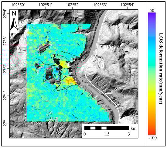
Figure 6.
Line-of-sight (LOS) deformation rate chart in 2023.
This study primarily analyses deformation near the Dawanzi tunnel. We find two distinct deformation zones, Zone I and Zone III, within the bank slope section where the tunnel is situated. By analyzing engineering geological zoning (see Figure 6) and time-series deformation results (see Figure 7), we observe differences in the distribution of deformation rates between these zones. Zone I shows a fan-shaped deformation along the 825 m water level line. It spans approximately 660 m in length with a leading edge width of about 680 m. Higher deformation rates occur in the coastal area and the prominent part of the middle and rear terrain. In contrast, Zone III exhibits an oblate shape, measuring around 890 m in length and 490 m in width at its widest point. The elevated deformation rates concentrate on the front bank collapse and the sub-landslide area on the right front side.
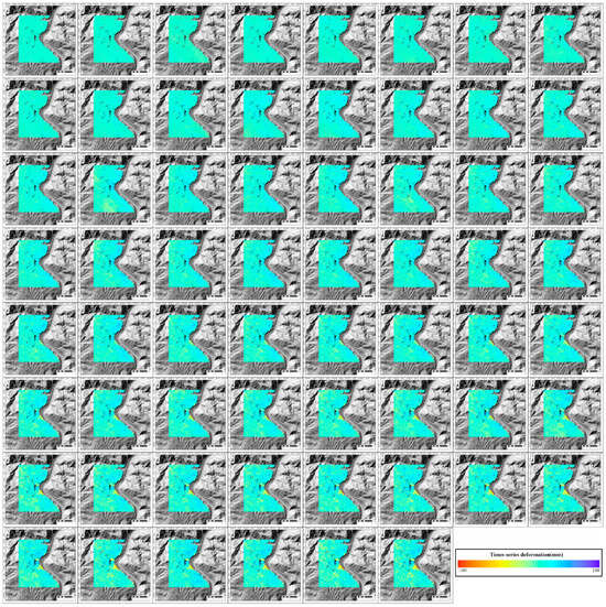
Figure 7.
The reference scene is the cumulative deformation map of the study area on 3 January 2021. There are 62 scenes from 3 January 2021 to 5 January 2023; they are also data for training and validation. There are clearer images in the Supplementary Materials, Figure S1.
The impoundment of Baihetan hydropower station commenced in April 2021 (refer to Figure 2). Within approximately three months of impoundment, it reached the current low water level of 775 m. The deformation of the bank slope beside the Jinsha River mainly starts from the data on 10 January 2022, and this period is the time when the water level is declining. Over time, the Dawanzi landslide consistently exhibits deformation away from the satellite. Analysis of Figure 2 and Figure 7 reveals a notable correlation between the water level fluctuations of the Jinsha River and the development of deformation within the landslide. As of 19 December 2023, the maximum deformation monitored by SBAS was −180 mm and 100 mm.
4.2. Time Series Deformation Prediction Results
Of the 86 data, only the first 74 can be used for model training and verification because of missing data in June–July 2023. To better show the training effect of the prediction model and verify it, we selected the data from 3 January 2021 to 5 January 2023 as the model of the training set. The data from 26 August 2022 to 5 January 2023 are used as the model’s input to obtain the prediction results from 17 January 2023 to 29 May 2023. The results are compared with the results obtained by the SBAS-InSAR, and the results are shown in Figure 8. The results generated by the Informer model are close to those obtained from the SBAS-InSAR method, exhibiting little difference to the naked eye. On 17 May 2023, the SBAS-InSAR method observed a slight blue-deepening phenomenon; however, upon comparison with results from preceding and subsequent periods, we attribute this to the influence of noise. It shows that noise has less influence on the forecasting results of our model.
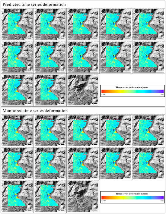
Figure 8.
Predicted and monitored time-series displacement maps from 17 January 2023, to 29 May 2023. There are clearer images in the Supplementary Materials, Figure S2.
To further demonstrate the predictive capabilities of our model, Figure 9c shows the cumulative deformation histogram for prediction and monitoring on 29 May 2023. We observe minimal difference between the prediction results and those obtained through the SBAS-InSAR method, especially in small deformation. Our model tends to yield more conservative results than the SBAS-InSAR method. The standard deviation of the two histograms is 0.0216, with average and median values of the model prediction results and SBAS-InSAR results being 3.3 mm and 3.6 mm, 4.7 mm and 5.3 mm, respectively. We analyze that the SBAS-InSAR method exhibits more deformation in the direction close to the sensor due to vegetation growth.
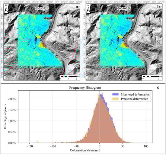
Figure 9.
Comparison between the predicted and monitored time series cumulative deformation maps on 29 May 2023. (a) The monitored deformation map. (b) The predicted deformation diagram (c) The cumulative deformation histogram. The (a,b) diagram is taken from Figure 8.
4.3. Deformation Analysis of Typical Points
To analyze the predictive capability of our model across different deformation regions, we randomly select six points with different conditions in Figure 10 and examine the deformation characteristics of each region. Among these points, points A and D are situated in Zone I, point B in Zone III, point C in the upper right bank landslide area of Zone IV, point E in Zone II, and point F in a non-deformation area distant from the Jinsha River. Figure 11 shows the line chart of time series deformation of the six points predicted by the Informer model. Landslide susceptibility is affected by various factors such as soil moisture, drainage distance, vegetation, and precipitation [46]. We compare the prediction results of univariate ablation experiments and those of the multivariate Informer model. This comparison aims to explain the impact of these factors on the prediction of reservoir bank slope deformation. The input data of the univariate ablation experiment based on the Informer model only contains time series deformation data.
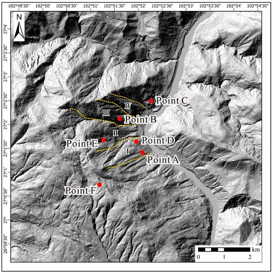
Figure 10.
Distribution of points. The background is the hillshade of the study area.
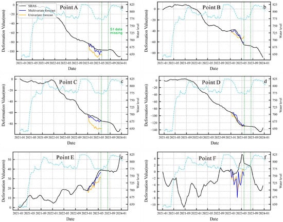
Figure 11.
Comparison of univariate and multivariate prediction results at each point. The blue and orange lines in (a) represent the same meaning as the rest of the images, and the dotted line of the sky blue is the waterline.
Figure 11 illustrates that the multivariate data more accurately approximates the deformation curves of the study area obtained by the SBAS-InSAR method than the univariate data, a conclusion evident in Figure 11a–c,e. Models trained on univariate data exhibit an “inertia”, as shown in Figure 11a,c,d. For more straightforward trends, such as when the pre-deformation information has a linear decreasing trend, this ‘inertia‘ will cause the model to fail to change accordingly when other factors change. The corresponding representation is that the univariate training model overestimates the deformation results in Figure 11a,c, and the deformation prediction in Figure 11b is conservative; however, the effect shown in Figure 11d is similar to the model trained by multivariate data. Even though the data of 86 periods are missing for two months, we can observe from the trend shown in the last 12 periods of these figures in Figure 11 that the prediction of the deformation trend by the model trained with multivariate data is highly reliable. The difference between multivariate and univariate prediction is insignificant for the F point with small deformation and far away from Jinsha River in SBAS-InSAR results. From Figure 11f, we can also observe that the small deformation data processed by the SBAS-InSAR method for S1 data over a long time series exhibit significant volatility, demonstrating low reliability. In summary, the influencing factors we selected significantly impact the deformation of the reservoir bank slope. This impact aids in predicting deformations in large deformation areas of the bank slope but has minimal effect on non-deformation areas.
Next, we will analyze the deformation characteristics of the regions represented by these six points. In Figure 11b, we observe that even at points A-E in the great deformation zone, only small deformation occurs before the water level reaches 816m for the first time in October 2021. However, significant deformation occurs at points A–E approximately two months after the water level begins to decline. This phenomenon is particularly typical at points B and C, and the same deformation acceleration also occurs during the decline of the water level after secondly reaching the high water level from January 2023 to May 2023; it indicates that the deformation of zones III and IV is more obviously affected by the water level. Zones I, where points A and D are located, except for being more affected by the water level during the initiation of the deformation, show a tendency to slow down the deformation in the last 12 periods of the data. Considering the engineering control situation and the region’s deformation characteristics, we predict that deformation will slow down or cease when the water level drops for the third time from its peak in December 2023. The relationship between deformation and water level change at point E is unclear. It shows a lifting of the ground surface, probably related to the change in buoyancy due to the change in water level. Point F is in a state of no deformation, and the deformation data only relates to the noise and vegetation.
5. Discussion
5.1. Informer Performance on This Dataset
We conducted a comparative study to assess the impact of the ProbSparse self-attention mechanism and self-attention distillation mechanism on the training effectiveness of our dataset. The results in Table 1 show that the ProbSparse self-attention mechanism and the self-attention mechanism in Transformer have similar effects, with nearly MSE and Mean Absolute Error (MAE) values. However, the self-attention distillation mechanism demonstrates a practical improvement in training our dataset. Furthermore, ProbSparse self-attention and self-attention distillation mechanisms exhibit excellent complexity and can predict more extended time series under similar hardware conditions [29].

Table 1.
Training effects of different mechanisms.
We trained and predicted using LSTM, RNN, GRU, and Informer models to evaluate our method’s accuracy of time series deformation prediction. Besides the loss function MSE, we used MAE, Root Mean Squared Error (RMSE), and MAPE to evaluate each model’s performance. The Informer model predicted values closely match those obtained by the SBAS-InSAR method, with a Mean Absolute Percentage Error (MAPE) of only 1.631%, indicating that the average difference between all predicted values and actual values is 1.631%, demonstrating the effectiveness of our prediction method. Table 2 shows that, for our dataset, the accuracy of the Informer model surpasses others. It suggests that the Informer model with ProbSparse self-attention mechanism performs better on sequences containing periodic fluctuation signals of water level. It can effectively handle long input sequences and achieve high deformation prediction performance at the point scale. Overall, the Informer model exhibits excellent performance and can effectively predict long-term series of surface deformation of reservoir bank slope.
Table 2.
The training results of the dataset in this paper on deep learning models.
This paper represents the first attempt to predict the deformation trend of the reservoir bank slope using the Transformer-based model. Due to the gradient disappearance and explosion problems in RNN or LSTM and the limitations of convolutional filters, they have limitations in modeling long-term complex relationships in sequence data. In contrast, the Informer model retains a direct link to all previous time stamps, allowing information to spread over a more extended sequence, which makes it suitable for the deformation prediction of long-time series. Moreover, our proposed method comprehensively considers various deformation factors of the bank slope, including rainfall, water level changes, drainage distance, and other information. By learning the deformation patterns of the bank slope, it achieves accurate prediction results. The time series deformation results capture essential signals of periodic changes around the bank slope, reflecting trends of sinking or rising over time due to rainfall and surface runoff effects. The prediction results depicted in Figure 11 demonstrate the method’s ability to simulate both water level-related and non-water level-related deformation signals accurately.
5.2. Limitations and Prospects
The main disadvantage of this method is that the trained results of one slope are not universal for other bank slopes. The time series features considered in the model, such as water level and drainage distance, are not the most critical factors affecting the deformation of the bank slope. It is difficult to quantitatively describe the rock formation and geological structures of pixels. Moreover, these characteristics are not time-varying. However, the location of the points in the dataset describes the factors that affect these factors. In other words, the location of the points represents the geological information of the pixel area. Since the calculation work of the time series prediction task is less than that of computer vision and natural language processing tasks, the Informer model has excellent computational complexity. So, it is practicable to recreate and train new models to analyze other bank slopes. Nevertheless, when using the dataset of another slope, it is essential to consider its richness. Finally, this method only applies to forecasting the slow-moving reservoir bank slope deformation.
Despite these limitations, there are several avenues for future research and improvements. Incorporating additional critical factors, such as geological characteristics and material properties, into the model could enhance its predictive accuracy and generalizability. Advanced techniques like transfer learning might be explored to adapt the model to different slopes without extensive retraining. Integrating more comprehensive datasets with diverse slope conditions and deformation patterns could also help create a more robust model. Future work could also focus on real-time monitoring and prediction, leveraging sensor data and Internet of Things (IoT) technology to provide more timely and precise forecasts. By addressing these challenges and expanding the model’s scope, we can significantly advance the application of time series analysis in geotechnical engineering and slope stability prediction.
6. Conclusions
This paper studies a time series prediction method for slope deformation using the Informer model, demonstrating its effectiveness in application to the Dawanzi landslide. The research proves that the model has great potential in predicting the deformation of the deformation zone of the reservoir bank slope. Based on the above research, we can draw the following conclusions:
- (1)
- The deformation rate in most parts of the study area is between −10 mm/year and 10 mm/year, and the maximum deformation rate detected around the bank slope is more than −100 mm/year;
- (2)
- Based on the Informer model, the displacement mode of the reservoir bank slope can be predicted. Compared with other existing methods, the model performs better in predicting the deformation trend of the reservoir bank slope. The RMSE and MAPE of the predicted displacement of the 144-day time series of 12 periods is 3.373 mm and 1.631%;
- (3)
- According to the deformation characteristics of the random points, we have the following understanding of the Dawanzi landslide: the four areas where the Dawanzi tunnel is located have obvious deformation in zones I and III. The start of the deformation of the two is related to the decline of the water level after the first impoundment. Zone III’s deformation rate strongly correlates with the water level change. We predict that the deformation in Zone III will remain slow or stop, and the deformation in Zone I will continue, but the rate will decrease.
In the future, to achieve more accurate prediction of bank slope deformation and improve the robustness of the prediction model. We will incorporate more data on the other reservoir bank slopes into the model, improve the model to consider the spatial relationship between different variables and learn the spatial and temporal relationship between deformation and other factors from the data.
Supplementary Materials
The following supporting information can be downloaded at https://www.mdpi.com/article/10.3390/rs16152688/s1. Table S1: Supplementary images overview; Figure S1: Images in Figure 7; Figure S2: Images in Figure 8.
Author Contributions
Q.L.: Drafting of the manuscript; improving the Informer; analysis and/or interpretation of data; building the datasets; SBAS-InSAR process. X.Y.: Critically revising the manuscript, mainly through discussions. Conception and design of the research. Z.Z.: Site investigation of the study area; SBAS-InSAR process. C.Y.: Site investigation of the study area. K.R.: Site investigation of the study area. All authors have read and agreed to the published version of the manuscript.
Funding
This research was funded by China Three Gorges Corporation YMJ(XLD)/(19)110; China Geology Survey Project (DD20230433); Project of Ministry and Province Cooperation (Sichuan Geohazard SCDZRS-2023).
Data Availability Statement
Data will be made available on request.
Acknowledgments
We thank China Three Gorges Corporation for funding.
Conflicts of Interest
The authors declare no conflicts of interest.
References
- Cheng, Z.; Liu, S.; Fan, X.; Shi, A.; Yin, K. Deformation Behavior and Triggering Mechanism of the Tuandigou Landslide around the Reservoir Area of Baihetan Hydropower Station. Landslides 2023, 20, 1679–1689. [Google Scholar] [CrossRef]
- Paronuzzi, P.; Rigo, E.; Bolla, A. Influence of Filling–Drawdown Cycles of the Vajont Reservoir on Mt. Toc Slope Stability. Geomorphology 2013, 191, 75–93. [Google Scholar] [CrossRef]
- Wu, S.; Hu, X.; Zheng, W.; Zhang, G.; Liu, C.; Xu, C.; Zhang, H.; Liu, Z. Displacement Behaviour and Potential Impulse Waves of the Gapa Landslide Subjected to the Jinping Reservoir Fluctuations in Southwest China. Geomorphology 2022, 397, 108013. [Google Scholar] [CrossRef]
- Xu, L.; Rong, G.; Qiu, Q.; Zhang, H.; Chen, W.; Chen, Z. Analysis of Reservoir Slope Deformation during Initial Impoundment at the Baihetan Hydropower Station, China. Eng. Geol. 2023, 323, 107201. [Google Scholar] [CrossRef]
- Zhou, Z.; Yao, X.; Li, R.; Jiang, S.; Zhao, X.; Ren, K.; Zhu, Y. Deformation Characteristics and Mechanism of an Impoundment-Induced Toppling Landslide in Baihetan Reservoir Based on Multi-Source Remote Sensing. J. Mt. Sci. 2023, 20, 3614–3630. [Google Scholar] [CrossRef]
- Mulas, M.; Ciccarese, G.; Truffelli, G.; Corsini, A. Integration of Digital Image Correlation of Sentinel-2 Data and Continuous GNSS for Long-Term Slope Movements Monitoring in Moderately Rapid Landslides. Remote Sens. 2020, 12, 2605. [Google Scholar] [CrossRef]
- Zajdel, R.; Sośnica, K.; Bury, G. A New Online Service for the Validation of Multi-GNSS Orbits Using SLR. Remote Sens. 2017, 9, 1049. [Google Scholar] [CrossRef]
- Kang, Y.; Lu, Z.; Zhao, C.; Xu, Y.; Kim, J.; Gallegos, A.J. InSAR Monitoring of Creeping Landslides in Mountainous Regions: A Case Study in Eldorado National Forest, California. Remote Sens. Environ. 2021, 258, 112400. [Google Scholar] [CrossRef]
- Kim, J.; Coe, J.A.; Lu, Z.; Avdievitch, N.N.; Hults, C.P. Spaceborne InSAR Mapping of Landslides and Subsidence in Rapidly Deglaciating Terrain, Glacier Bay National Park and Preserve and Vicinity, Alaska and British Columbia. Remote Sens. Environ. 2022, 281, 113231. [Google Scholar] [CrossRef]
- Aswathi, J.; Kumar, R.B.; Oommen, T.; Bouali, E.H.; Sajinkumar, K.S. InSAR as a Tool for Monitoring Hydropower Projects: A Review. Energy Geosci. 2022, 3, 160–171. [Google Scholar] [CrossRef]
- Li, L.; Yao, X.; Yao, J.; Zhou, Z.; Feng, X.; Liu, X. Analysis of Deformation Characteristics for a Reservoir Landslide before and after Impoundment by Multiple D-InSAR Observations at Jinshajiang River, China. Nat Hazards 2019, 98, 719–733. [Google Scholar] [CrossRef]
- Zhao, C.; Kang, Y.; Zhang, Q.; Lu, Z.; Li, B. Landslide Identification and Monitoring along the Jinsha River Catchment (Wudongde Reservoir Area), China, Using the InSAR Method. Remote Sens. 2018, 10, 993. [Google Scholar] [CrossRef]
- Dwivedi, R.; Narayan, A.B.; Tiwari, A.; Dikshit, O.; Singh, A.K. Multi-Temporal SAR Interferometry for Landslide Monitoring. Int. Arch. Photogramm. Remote Sens. Spat. Inf. Sci. 2016, 41, 55–58. [Google Scholar] [CrossRef]
- Reyes-Carmona, C.; Barra, A.; Galve, J.P.; Monserrat, O.; Pérez-Peña, J.V.; Mateos, R.M.; Notti, D.; Ruano, P.; Millares, A.; López-Vinielles, J. Sentinel-1 DInSAR for Monitoring Active Landslides in Critical Infrastructures: The Case of the Rules Reservoir (Southern Spain). Remote Sens. 2020, 12, 809. [Google Scholar] [CrossRef]
- Li, L.; Wen, B.; Yao, X.; Zhou, Z.; Zhu, Y. InSAR-Based Method for Monitoring the Long-Time Evolutions and Spatial-Temporal Distributions of Unstable Slopes with the Impact of Water-Level Fluctuation: A Case Study in the Xiluodu Reservoir. Remote Sens. Environ. 2023, 295, 113686. [Google Scholar] [CrossRef]
- Dun, J.; Feng, W.; Yi, X.; Zhang, G.; Wu, M. Detection and Mapping of Active Landslides before Impoundment in the Baihetan Reservoir Area (China) Based on the Time-Series InSAR Method. Remote Sens. 2021, 13, 3213. [Google Scholar] [CrossRef]
- Ramirez, R.A.; Abdullah, R.E.E.; Rubio, C.J.P. S1-Psinsar Monitoring and Hyperbolic Modeling of Nonlinear Ground Subsidence in Naga City, Cebu Island in the Philippines. Geomate J. 2022, 23, 102–109. [Google Scholar] [CrossRef]
- Intrieri, E.; Carlà, T.; Gigli, G. Forecasting the Time of Failure of Landslides at Slope-Scale: A Literature Review. Earth-Sci. Rev. 2019, 193, 333–349. [Google Scholar] [CrossRef]
- Newcomen, W.; Dick, G. An Update to Strain-Based Pit Wall Failure Prediction Method and a Justification for Slope Monitoring. Proc. Slope Stab. 2015, 139–150. [Google Scholar]
- Saito, M. Forecasting Time of Slope Failure by Tertiary Creep. In Proceedings of the 7th International Conference on Soil Mechanics and Foundation Engineering, Mexico City, Mexico, 25–29 August 1969; Volume 2, pp. 677–683. [Google Scholar]
- Voight, B. A Relation to Describe Rate-Dependent Material Failure. Science 1989, 243, 200–203. [Google Scholar] [CrossRef]
- Du, J.; Yin, K.; Lacasse, S. Displacement Prediction in Colluvial Landslides, Three Gorges Reservoir, China. Landslides 2013, 10, 203–218. [Google Scholar] [CrossRef]
- Zhou, C.; Cao, Y.; Gan, L.; Wang, Y.; Motagh, M.; Roessner, S.; Hu, X.; Yin, K. A Novel Framework for Landslide Displacement Prediction Using MT-InSAR and Machine Learning Techniques. Eng. Geol. 2024, 334, 107497. [Google Scholar] [CrossRef]
- Hill, P.; Biggs, J.; Ponce-López, V.; Bull, D. Time-Series Prediction Approaches to Forecasting Deformation in Sentinel-1 InSAR Data. JGR Solid Earth 2021, 126, e2020JB020176. [Google Scholar] [CrossRef]
- Radford, A.; Wu, J.; Child, R.; Luan, D.; Amodei, D.; Sutskever, I. Language Models Are Unsupervised Multitask Learners. OpenAI Blog 2019, 1, 9. [Google Scholar]
- Vaswani, A.; Shazeer, N.; Parmar, N.; Uszkoreit, J.; Jones, L.; Gomez, A.N.; Kaiser, Ł.; Polosukhin, I. Attention Is All You Need. Adv. Neural Inf. Process. Syst. 2017, 30. [Google Scholar]
- Wen, Q.; Zhou, T.; Zhang, C.; Chen, W.; Ma, Z.; Yan, J.; Sun, L. Transformers in Time Series: A Survey. arXiv 2023, arXiv:2202.07125. [Google Scholar]
- Wang, J.; Li, C.; Li, L.; Huang, Z.; Wang, C.; Zhang, H.; Zhang, Z. InSAR Time-Series Deformation Forecasting Surrounding Salt Lake Using Deep Transformer Models. Sci. Total Environ. 2023, 858, 159744. [Google Scholar] [CrossRef] [PubMed]
- Zhou, H.; Zhang, S.; Peng, J.; Zhang, S.; Li, J.; Xiong, H.; Zhang, W. Informer: Beyond Efficient Transformer for Long Sequence Time-Series Forecasting. In Proceedings of the AAAI Conference on Artificial Intelligence, Online, 2–9 February 2021. [Google Scholar]
- DeBo, L.; ChangQing, Z.; ChengDong, S.; Huan, L. Role of Regional Geochemical Survey for Ge Mineral Prediction in Chuan-Dian-Qian Pb-Zn (Ge) Metallogenic Region. Acta Petrol. Sin. 2019, 35, 3407–3428. [Google Scholar] [CrossRef]
- Liu, W.; Hu, K.; Carling, P.A.; Lai, Z.; Cheng, T.; Xu, Y. The Establishment and Influence of Baimakou Paleo-Dam in an Upstream Reach of the Yangtze River, Southeastern Margin of the Tibetan Plateau. Geomorphology 2018, 321, 167–173. [Google Scholar] [CrossRef]
- Yang, Z.; Xi, W.; Yang, Z.; Shi, Z.; Huang, G.; Guo, J.; Yang, D. Time-Lag Response of Landslide to Reservoir Water Level Fluctuations during the Storage Period: A Case Study of Baihetan Reservoir. Water 2023, 15, 2732. [Google Scholar] [CrossRef]
- Torres, R.; Snoeij, P.; Geudtner, D.; Bibby, D.; Davidson, M.; Attema, E.; Potin, P.; Rommen, B.; Floury, N.; Brown, M. GMES Sentinel-1 Mission. Remote Sens. Environ. 2012, 120, 9–24. [Google Scholar] [CrossRef]
- Hersbach, H.; Bell, B.; Berrisford, P.; Hirahara, S.; Horányi, A.; Muñoz-Sabater, J.; Nicolas, J.; Peubey, C.; Radu, R.; Schepers, D.; et al. The ERA5 Global Reanalysis. Quart. J. Royal Meteoro. Soc. 2020, 146, 1999–2049. [Google Scholar] [CrossRef]
- Beck, P.S.; Atzberger, C.; Høgda, K.A.; Johansen, B.; Skidmore, A.K. Improved Monitoring of Vegetation Dynamics at Very High Latitudes: A New Method Using MODIS NDVI. Remote Sens. Environ. 2006, 100, 321–334. [Google Scholar] [CrossRef]
- Wang, D.; Morton, D.; Masek, J.; Wu, A.; Nagol, J.; Xiong, X.; Levy, R.; Vermote, E.; Wolfe, R. Impact of Sensor Degradation on the MODIS NDVI Time Series. Remote Sens. Environ. 2012, 119, 55–61. [Google Scholar] [CrossRef]
- Massonnet, D.; Feigl, K.L. Radar Interferometry and Its Application to Changes in the Earth’s Surface. Rev. Geophys. 1998, 36, 441–500. [Google Scholar] [CrossRef]
- Hanssen, R.F. Radar Interferometry: Data Interpretation and Error Analysis; Springer Science & Business Media: Berlin/Heidelberg, Germany, 2001; Volume 2. [Google Scholar]
- Biggs, J.; Wright, T.; Lu, Z.; Parsons, B. Multi-Interferogram Method for Measuring Interseismic Deformation: Denali Fault, Alaska. Geophys. J. Int. 2007, 170, 1165–1179. [Google Scholar] [CrossRef]
- Confuorto, P.; Di Martire, D.; Centolanza, G.; Iglesias, R.; Mallorqui, J.J.; Novellino, A.; Plank, S.; Ramondini, M.; Thuro, K.; Calcaterra, D. Post-Failure Evolution Analysis of a Rainfall-Triggered Landslide by Multi-Temporal Interferometry SAR Approaches Integrated with Geotechnical Analysis. Remote Sens. Environ. 2017, 188, 51–72. [Google Scholar] [CrossRef]
- Wegnüller, U.; Werner, C.; Strozzi, T.; Wiesmann, A.; Frey, O.; Santoro, M. Sentinel-1 Support in the GAMMA Software. Procedia Comput. Sci. 2016, 100, 1305–1312. [Google Scholar] [CrossRef]
- Berardino, P.; Fornaro, G.; Lanari, R.; Sansosti, E. A New Algorithm for Surface Deformation Monitoring Based on Small Baseline Differential SAR Interferograms. IEEE Trans. Geosci. Remote Sens. 2002, 40, 2375–2383. [Google Scholar] [CrossRef]
- Chen, J.; Wu, T.; Liu, L.; Gong, W.; Zwieback, S.; Zou, D.; Zhu, X.; Hu, G.; Du, E.; Wu, X.; et al. Increased Water Content in the Active Layer Revealed by Regional-Scale InSAR and Independent Component Analysis on the Central Qinghai-Tibet Plateau. Geophys. Res. Lett. 2022, 49, e2021GL097586. [Google Scholar] [CrossRef]
- Tsai, Y.-H.H.; Bai, S.; Liang, P.P.; Kolter, J.Z.; Morency, L.-P.; Salakhutdinov, R. Multimodal Transformer for Unaligned Multimodal Language Sequences. In Proceedings of the Association for Computational Linguistics Meeting, Florence, Italy, 28 July–2 August 2019; NIH Public Access. Volume 2019, p. 6558. [Google Scholar]
- Kingma, D.P.; Ba, J. Adam: A Method for Stochastic Optimization. arXiv 2017, arXiv:1412.6980. [Google Scholar]
- Kavzoglu, T.; Kutlug Sahin, E.; Colkesen, I. Selecting Optimal Conditioning Factors in Shallow Translational Landslide Susceptibility Mapping Using Genetic Algorithm. Eng. Geol. 2015, 192, 101–112. [Google Scholar] [CrossRef]


Disclaimer/Publisher’s Note: The statements, opinions and data contained in all publications are solely those of the individual author(s) and contributor(s) and not of MDPI and/or the editor(s). MDPI and/or the editor(s) disclaim responsibility for any injury to people or property resulting from any ideas, methods, instructions or products referred to in the content. |
© 2024 by the authors. Licensee MDPI, Basel, Switzerland. This article is an open access article distributed under the terms and conditions of the Creative Commons Attribution (CC BY) license (https://creativecommons.org/licenses/by/4.0/).