Power Allocation Scheme for Multi-Static Radar to Stably Track Self-Defense Jammers

Abstract

Due to suppression jamming by jammers, the signal-to-interference-plus-noise ratio (SINR) during tracking tasks is significantly reduced, thereby decreasing the target detection probability of radar systems. This may result in the interruption of the target track. To address this issue, we propose a multi-static radar power allocation algorithm that enhances the detection and tracking performance of multiple radars in relation to their targets by optimizing power resource allocation. Initially, the echo signal model and measurement model of multi-static radar are formulated, followed by the derivation of the Bayesian Cramér–Rao lower bound (BCRLB). The multi-objective optimization method is utilized to establish the objective function for joint tracking and detection, with dynamic adjustment of the weight coefficient to balance the tracking and detection performance of multiple radars. This ensures the reliability and anti-jamming capability of the multi-static radar system. Simulation results indicate that the proposed algorithm can prevent the interruption of jammer tracking and maintain robust tracking performance.

1. Introduction

MIMO radar can transmit uncorrelated or orthogonal signals by using multiple transmitter antennas and receiver antennas [1,2]. Compared with the conventional phased-array radar, MIMO radar possesses superior spatial diversity and waveform diversity, which contribute to its advantages in target detection [3], tracking [4], parameter estimation [5,6], and anti-interference [7,8]. However, in modern electronic warfare (EW), the performance of radar systems is restricted to a certain extent due to the existence of enemy jamming. In practice, efficient resource management strategies can mitigate the impact of this jamming on radar systems [9,10,11].

In practical applications, the thorough use of resources can improve task performance, but it often results in the unnecessary consumption of system resources. Optimal resource allocation enables the achievement of similar system performance with fewer resources [12,13,14], thereby decreasing the system’s computational complexity and increasing overall efficiency. Current research can be broadly classified into two categories: selection and configuration of array elements based on system architecture, and resource allocation based on launch parameters.

For system structure optimization, researchers modeled the antenna selection problem as a knapsack problem (KP) [15] and used a heuristic algorithm to implement antenna subset selection. In [16], the authors used sparse antenna array configurations to alleviate spectrum congestion and competition over frequency bandwidth in dual-function radar–communications systems. In [17], the authors proposed a suboptimal two-step second-order cone programming solution to conserve transmitter numbers and minimize the error in estimating target position using MIMO radar sensor networks. Refs. [18,19] utilized limited antennas for tracking multiple targets on the basis of improving the overall tracking accuracy.

The research results of the second type of resource optimization have mainly focused on power allocation. In [20,21], the authors used an optimization technique to control the limited beam and power resource to achieve accurate estimation of the target state. In [22], based on cooperative game theory, the power allocation problem of distributed MIMO radar for target tracking was studied. In [23], based on the estimate of the signal-to-interference-plus-noise ratio (SINR), the authors incorporated convex optimization methods and non-cooperative game-theoretic techniques to solve the power allocation problem for a multi-static MIMO radar network.

In [24], the authors firstly studied the Cramér–Rao lower bound (CRLB) of the direction-of-arrival (DOA) estimate. In [25], the authors derived the CRLB of the joint DOA and Doppler frequency in the situation of transmitting the coherent pulse train. In [26], the analytical expression for the predicted BCRLB was derived, which was employed to evaluate the target tracking accuracy. In [12], covariance intersection (CI) fusion was employed in a distributed fusion architecture and the BCRLB for the CI fusion rule was derived.

Stable tracking via radar systems is based on the effective detection of the target. In practice, due to suppression jamming released by jammers and other factors, the detection probability of the radar in relation to the target may be less than 1, which potentially results in missed detections and even target-tracking interruptions in severe cases [27]. To solve this issue, we propose a multi-objective optimization algorithm, which can improve the probability of detecting the target while maintaining tracking accuracy. The main contributions of this paper are as follows:

(1)

We establish a jamming signal model, an echo model, and a measurement model of multi-static radar. The BCRLB of joint time delay and Doppler frequency is derived to characterize the tracking accuracy. In addition, the SINR of each radar is used as an optimization function to characterize the detection accuracy. As a result, the limited power resources of the multi-static radar network are allocated efficiently to minimize the worst BCRLB and optimize the detection probability.

(2)

We propose a multi-objective optimization algorithm to solve the power allocation problem of multi-static radar. The BCRLB and detection probability of each radar are simultaneously used as the optimization index, with varying weight coefficients assigned based on their significance. In order to maintain the target track continuity, these weight coefficients are dynamically adjusted according to the target detection probability across multiple frames.

(3)

Simulation results show that the proposed algorithm can achieve good tracking performance and detection performance compared with three other algorithms. For targets with low detection probability across multiple frames, the proposed algorithm adjusts its weight coefficient to improve the detection probability in the next frame, thereby ensuring target track continuity. In addition, two target reflection models are used to verify the effectiveness of the proposed algorithm.

The remainder of this paper is organized as follows. The system models are depicted in Section 2. In Section 3, the BCRLB with power allocation is derived for target tracking. In Section 4, the optimization problem is established and a multi-objective optimization algorithm is proposed as a solution to the problem. The simulation results and conclusion are presented in Section 5 and Section 6, respectively.

2. System Model

2.1. Jamming Signal Model

Assuming that the self-defense jammer generates a noise frequency modulation (FM) jamming signal and can simultaneously saturate multiple receivers with electromagnetic noise, the jamming signal received by the m-th radar can be expressed as

$$j_{m,k}^q(t)=\sqrt{P_{m,k,q}^J}\exp [-j2\pi (w_0(t-{\tau }_{m,k}^{q,J})+2\pi K_{\mathrm{fm}}\underset{0}{\overset{t}{\int }}\xi (t-{\tau }_{m,k}^{q,J})\mathrm{d}t+{\phi }_0)]$$

(1)

where $w_0$, $K_{\mathrm{fm}}$, ${\tau }_{m,k}^{q,J}=R_{m,k}^q/c$, and ${\phi }_0$ represent the center frequency, the chirp rate, the time delay, and the initial phase, respectively. $\xi (t)$ denotes the modulation noise and is assumed to be zero-mean Gaussian with a known covariance ${\sigma }_{\xi }^2$, and $P_{m,k,q}^J$ denotes the jamming power and can be expressed as

$$P_{m,k,q}^J={\displaystyle \frac{P_{m,k,q}{\tau }_c^J{G}_t^J{({\lambda }^J)}^2\gamma }{{\left(4\mathsf{\pi }\right)}^3{(R_{m,k}^q)}^2}}$$

(2)

where $R_{m,k}^q$ denotes the radial distance from the m-th radar to the q-th target; $P_{m,k,q}$, ${\lambda }^J$, $G_t^J$, $\gamma$, and ${\tau }_c^J$ denote the jamming signal transient power, the carrier wavelength of jamming signal, the transmitter antenna gain of the jammer, polarization mismatch loss, and effective pulse width in a single exposure period, respectively.

2.2. Radar Signal Model

Without loss of generality, we consider a multi-static radar network with M separate radars. These radars are labeled $1,2,\cdots ,M\ge 2$ with the location of the m-th radar denoted by $\left(x_m,y_m\right)$. In the kth sample interval, the m-th radar transmits the normalized orthogonal signal:

$${\displaystyle {\int }_{-\infty }^{+\infty }{\left|{\tilde{s}}_m\left(t\right)\right|}^2\mathrm{d}t=1}$$

(3)

$${\displaystyle {\int }_{-\infty }^{+\infty }{\tilde{s}}_m\left(t\right){\tilde{s}}_{m^{\prime }}^{\mathrm{H}}\left(t-\tau \right)\mathrm{d}t=\left\{\begin{array}{l}0,m\ne m^{\prime }\\ 1,m=m^{\prime }\end{array}\right.}$$

(4)

The effective bandwidth and effective time width of the signal can be expressed as

$${\beta }_m=\left({\displaystyle \int f^2{\left|S_m\left(f\right)\right|}^2\mathrm{d}f}\right)/\left({\displaystyle \int {\left|S_m\left(f\right)\right|}^2\mathrm{d}f}\right)$$

(5)

$$T_m=\left({\displaystyle \int t^2{\left|{\tilde{s}}_m\left(t\right)\right|}^2\mathrm{d}t}\right)/\left({\displaystyle \int {\left|{\tilde{s}}_m\left(t\right)\right|}^2\mathrm{d}t}\right)$$

(6)

where $S_m\left(f\right)$ denotes the Fourier transform of ${\tilde{s}}_m\left(t\right)$. The echo signal of multi-static radar can be expressed as

$$r_{m,k}^q\left(t\right)=h_{m,k}^q\sqrt{P_{m,k,q}^r}{\tilde{s}}_m\left(t-{\tau }_{m,k}^q\right){\mathrm{e}}^{-\mathrm{j}2\mathsf{\pi }{f}_{\mathrm{d}m,k}^{q}t}+j_{m,k}^q(t)+n_m\left(t\right)$$

(7)

where $h_{m,k}^q$ denotes the complex gain of target reflectivity. ${\tau }_{m,k}^q=2R_{m,k}^q/c$ and $f_{\mathrm{d}m,k}^q$ denote the time delay and the Doppler frequency. $n_m\left(t\right)$ denotes the complex Gaussian noise and is assumed to be zero-mean Gaussian with a known covariance ${\sigma }_m^2$. $P_{m,k,q}^r$ is the echo signal power:

$$P_{m,k,q}^r={\displaystyle \frac{P_{\mathrm{t}m,k}{\tau }_{\mathrm{c}}{(G_{\mathrm{t}})}^2{I}_{\mathrm{p}}{\lambda }^2}{{\left(4\mathsf{\pi }\right)}^3{(R_{m,k}^q)}^4}}$$

(8)

where $P_{\mathrm{t}m,k}$, ${\tau }_{\mathrm{c}}$, $G_{\mathrm{t}}$, $I_p$, and $\lambda$ denote the transmit power, effective pulse width in a single exposure period, the antenna gain, receiver processing gain, and the carrier wavelength, respectively.

2.3. Motion Mode and Measurement Model

Assuming that there are $Q$ jammers in the region of interest (ROI) of the multi-static radar, and the jammer motion follows the nearly constant velocity (NCV) model in the 2-D space, with

$$x_k^q=F{x}_{\left.k\right|k-1}^q+w_k^q$$

(9)

where $x_k^q={\left[x_k^q,y_k^q,{\dot{x}}_k^q,{\dot{y}}_k^q\right]}^{\mathrm{T}}$, which denotes the state of q-th jammer. $F$ and $w_k^q~N\left(0,Q\right)$ denote the state transition matrix and the process noise matrix.

$$F=\left[\begin{array}{cc}1& T_{\mathrm{s}}\\ 0& 1\end{array}\right]\otimes I_2$$

(10)

$$Q=n_{\mathrm{f}}\left[\begin{array}{cc}{T}_{\mathrm{s}}^3/3& T_{\mathrm{s}}^2/2\\ T_{\mathrm{s}}^2/2& T_{\mathrm{s}}\end{array}\right]\otimes I_2$$

(11)

where $T_{\mathrm{s}}$, $I_2$, $\otimes$, and $n_{\mathrm{f}}$ denote sample interval, the second order identity matrix, the Kronecker product operator, and the noise intensity, respectively.

The probability of the m-th radar detecting the q-th jammer can be expressed as [28]

$$P_{{\mathrm{d}}_{q,k}}^m=Q\left(\sqrt{2{\chi }_{q,k}^m},\sqrt{-2\ln P_{\mathrm{fa}}}\right)$$

(12)

where $Q\left(\cdot \right)$, ${\chi }_{q,k}^m$, and $P_{\mathrm{fa}}$ represent the Marcum Q-function, signal-to-noise ratio and false-alarm probability.

We focus on the time delay and Doppler frequency of the jammers, which can be obtained by maximum likelihood estimation in the signals received by the multi-static radar network [29]. Assuming that the measurement is obtained under linear conditions, the measurement function can be written as

$$z_k^q=H{x}_k^q+v_k^q$$

(13)

where $H$ and $v_k^q~N\left(0,R_k^q\right)$ denote the $4\times 4$ identity matrix and the measurement noise vector. $R_k^q$ is the function of CRLB for the joint estimation of time delay and Doppler frequency, which will be introduced later. In this paper, the Kalman filter is used to estimate the jammer state.

3. Bayesian Cramér–Rao Lower Bound

All received signals are expressed in vector form:

$$r_k^q={\left[r_{1,k}^q,r_{2,k}^q\dots ,r_{M,k}^q\right]}^{\mathrm{T}}$$

(14)

The BCRLB provides the lowest bound for any unbiased estimator. Assuming that $f\left(r_k^q\right)$ is the unbiased estimate for $x_k^q$, then we have [30]

$${\mathbb{E}}_{x_k^q,r_k^q}\left\{\left[f\left(r_k^q\right)-x_k^q\right]{\left[f\left(r_k^q\right)-x_k^q\right]}^{\mathrm{T}}\right\}\ge J^{-1}\left(x_k^q\right)$$

(15)

where ${\mathbb{E}}_{x_k^q,r_k^q}$ denotes the operation of taking the mean value of the jammer state $x_k^q$ and observation value $r_k^q$. $J\left(x_k^q\right)$ denotes the Bayesian information matrix (BIM) for jammer tracking and can be written as

$$J\left(x_k^q\right)=-{\mathbb{E}}_{x_k^q,r_k^q}\left[{\nabla }_{x_k^q}^{x_k^q}\ln p\left(r_k^q,x_k^q\right)\right]$$

(16)

where ${\nabla }_{\eta }^{\nu }={\nabla }_{\eta }{\nabla }_{\nu }^T$ denotes the second-order partial derivative of a vector.

By blocking BIM, (16) can be expressed as [30]

$$J\left(x_k^q\right)=J_{\mathrm{P}}\left(x_k^q\right)+J_{\mathrm{D}}\left(x_k^q\right)$$

(17)

where $J_{\mathrm{P}}\left(x_k^q\right)$ denotes the Fisher information (FIM) of the prior information. $J_{\mathrm{D}}\left(x_k^q\right)$ denotes the FIM of the data:

$$\left\{\begin{array}{l}{J}_{\mathrm{P}}\left(x_k^q\right)=-{\mathbb{E}}_{x_k^q}\left[{\nabla }_{x_k^q}^{x_k^q}\ln p\left(x_k^q\right)\right]=\left[D_{k-1}^{22}-D_{k-1}^{21}{\left(J\left(x_{k-1}^q\right)+D_{k-1}^{11}\right)}^{-1}{D}_{k-1}^{12}\right]\\ J_{\mathrm{D}}\left(x_k^q\right)=-{\mathbb{E}}_{x_k^q,r_k^q}\left[{\nabla }_{x_k^q}^{x_k^q}\ln p\left(\left.r_k^q\right|x_k^q\right)\right]\end{array}\right.$$

(18)

where

$$\left\{\begin{array}{l}{D}_{k-1}^{11}=-{\mathbb{E}}_{x_{k-1}^q,x_k^q}\left[{\nabla }_{x_{k-1}^q}^{x_{k-1}^q}\ln p\left(\left.x_k^q\right|x_{k-1}^q\right)\right]\\ D_{k-1}^{12}=-{\mathbb{E}}_{x_{k-1}^q,x_k^q}\left[{\nabla }_{x_k^q}^{x_{k-1}^q}\ln p\left(\left.x_k^q\right|x_{k-1}^q\right)\right]={\left(D_{k-1}^{21}\right)}^{\mathrm{T}}\\ D_{k-1}^{22}=-{\mathbb{E}}_{x_{k-1}^q,x_k^q}\left[{\nabla }_{x_k^q}^{x_k^q}\ln p\left(\left.x_k^q\right|x_{k-1}^q\right)\right]\end{array}\right.$$

(19)

For the jammer motion described in (9), the three terms in (19) can easily be obtained by dropping out the expectation operator:

$$\left\{\begin{array}{l}{D}_{k-1}^{11}=F^{\mathrm{T}}{Q}^{-1}F\\ D_{k-1}^{12}=-F^{\mathrm{T}}{Q}^{-1}\\ D_{k-1}^{22}=Q^{-1}\end{array}\right.$$

(20)

Substituting (20) into the first term of (18), and using the matrix inverse lemma, $J_{\mathrm{P}}\left(x_k^q\right)$ is obtained as

$$J_{\mathrm{P}}\left(x_k^q\right)={\left[Q+F{J}^{-1}\left(x_{k-1}^q\right)F^{\mathrm{T}}\right]}^{-1}$$

(21)

As for $J_{\mathrm{D}}\left(x_k^q\right)$, we have

$$\begin{array}{ll}{J}_{\mathrm{D}}\left(x_k^q\right)& ={\left(R_k^q\right)}^{-1}={\mathbb{E}}_{x_k^q,r_k^q}\left[-{\nabla }_{x_k^q}^{x_k^q}\ln p\left(\left.r_k^q\right|x_k^q\right)\right]\\ & ={\mathbb{E}}_{x_k^q}\left\{{\mathbb{E}}_{\left.r_k^q\right|x_k^q}\left[-{\nabla }_{x_k^q}^{x_k^q}\ln p\left(\left.r_k^q\right|x_k^q\right)\right]\right\}\\ & ={\mathbb{E}}_{x_k^q}\left[{\left(A_k^q\right)}^{\mathrm{T}}{J}_{\mathrm{D}}\left({\theta }_k^q\right)A_k^q\right]\end{array}$$

(22)

where ${\theta }_k^q={\left[{\tau }_k^q,f_{\mathrm{d}k}^q\right]}^{\mathrm{T}}$, ${\tau }_k^q=\left[{\tau }_{1,k}^q,\dots ,{\tau }_{M,k}^q\right]$, $f_{\mathrm{d}k}^q=\left[f_{\mathrm{d}1,k}^q,\dots ,f_{\mathrm{d}M,k}^q\right]$, and $A_k^q$ represents the Jacobian matrix:

$$A_k^q={\left[A_{\tau },A_{f_{\mathrm{d}}}\right]}^{\mathrm{T}}$$

(23)

where

$$A_{\tau m}={\displaystyle \frac{2}{c}}\left[\begin{array}{c}\cos {\varphi }_{m,k}^q\\ \sin {\varphi }_{m,k}^q\\ 0\\ 0\end{array}\right]$$

(24)

$$A_{f_{\mathrm{d}}m}=-{\displaystyle \frac{4\mathsf{\pi }}{\lambda }}\left[\begin{array}{c}{\displaystyle \frac{-{\dot{x}}_k{\sin }^2{\varphi }_{m,k}^q+\frac{1}{2}{\dot{y}}_k\sin 2{\varphi }_{m,k}^q}{R_{m,k}^q}}\\ {\displaystyle \frac{-{\dot{y}}_k{\cos }^2{\varphi }_{m,k}^q+\frac{1}{2}{\dot{x}}_k\sin 2{\varphi }_{m,k}^q}{R_{m,k}^q}}\\ -\cos {\varphi }_{m,k}^q\\ -\sin {\varphi }_{m,k}^q\end{array}\right]$$

(25)

where $A_{\tau m}$ and $A_{f_{\mathrm{d}}m}$ are the m-th column matrix blocks in $A_{\tau }$ and $A_{f_{\mathrm{d}}}$ respectively. ${\varphi }_{m,k}^q$ in (24) and (25) is the angle between the q-th jammer and the m-th radar relative to the x-axis direction:

$${\varphi }_{m,k}^q=\arctan \left({\displaystyle \frac{y_k^q-y_m}{x_k^q-x_m}}\right)$$

(26)

Because the echo signals through each path are independent of each other, the FIM for ${\theta }_k^q$ can be written in matrix block form:

$$\begin{array}{ll}{J}_{\mathrm{D}}\left({\theta }_k^q\right)& =\left[\begin{array}{cc}{\mathbb{E}}_{\left.{\theta }_k^q\right|x_k^q}\left[-{\nabla }_{{\tau }_k^q}^{{\tau }_k^q}\ln p\left(\left.z_k^q\right|x_k^q\right)\right]& {\mathbb{E}}_{\left.{\theta }_k^q\right|x_k^q}\left[-{\nabla }_{f_{\mathrm{d}k}^q}^{{\tau }_k^q}\ln p\left(\left.z_k^q\right|x_k^q\right)\right]\\ {\mathbb{E}}_{\left.{\theta }_k^q\right|x_k^q}\left[-{\nabla }_{{\tau }_k^q}^{f_{\mathrm{d}k}^q}\ln p\left(\left.z_k^q\right|x_k^q\right)\right]& {\mathbb{E}}_{\left.{\theta }_k^q\right|x_k^q}\left[-{\nabla }_{f_{\mathrm{d}k}^q}^{f_{\mathrm{d}k}^q}\ln p\left(\left.z_k^q\right|x_k^q\right)\right]\end{array}\right]\\ & =\left[\begin{array}{cc}diag\left(8{\mathsf{\pi }}^2{\left(h_{m,k}^q\right)}^2{\beta }_m^{2}SNJ{R}_{m,k}^q\right)& 0\\ 0& diag\left(8{\mathsf{\pi }}^2{\left(h_{m,k}^q\right)}^2{T}_m^{2}SNJ{R}_{m,k}^q\right)\end{array}\right]\end{array}$$

(27)

where $diag\left(.\right)$ denotes the $M\times M$ diagonal matrix and $SNJ{R}_{m,k}^q$ denotes the SINR in the m-th radar for the q-th jammer, which is computed as follows:

$${\mathrm{SINR}}_{m,k,q}={\displaystyle \frac{P_{m,k,q}^r}{P_{m,k,q}^J+P_{m,k}^n}}$$

(28)

where $P_{m,k}^n$ is the intensity of internal noise at the receiver end. Then, (16) can be rewritten as

$$J\left(x_k^q\right)={\left[Q+F{J}^{-1}\left(x_{k-1}^q\right)F^{\mathrm{T}}\right]}^{-1}+{\mathbb{E}}_{x_k^q}\left[{\left(A_k^q\right)}^{\mathrm{T}}{J}_{\mathrm{D}}\left({\theta }_k^q\right)A_k^q\right]$$

(29)

From the derivation process, it can be seen that $J_{\mathrm{P}}\left(x_k^q\right)$ is related to only the jammer motion model, and the power allocation affects the BCRLB through influencing ${\mathrm{SINR}}_{m,k,q}$ and $J_{\mathrm{D}}\left(x_k^q\right)$. However, the main problem of (29) is that we must implement a large number of Monte Carlo simulations to evaluate the BIM and achieve the BCRLB, which would consume too much time. To satisfy the real-time demand of radar system, (29) can be rewritten as

$$J\left(x_k^q\right)={\left[Q+F{J}^{-1}\left(x_{k-1}^q\right)F^{\mathrm{T}}\right]}^{-1}+{\left({\widehat{A}}_k^q\right)}^{\mathrm{T}}{J}_{\mathrm{D}}\left({\widehat{\theta }}_k^q\right){\widehat{A}}_k^q$$

(30)

where ${\widehat{A}}_k^q$ and $J_{\mathrm{D}}\left({\widehat{\theta }}_k^q\right)$ are the Jacobian matrix and measurement covariance matrix evaluated around the prediction state vector ${\widehat{x}}_{\left.k\right|k-1}^q$.

If $P_k=\{P_{t1,k},P_{t2,k},\cdots ,P_{tM,k}\}$ is defined as the transmit power set of all radars in the multi-static radar network, the tracking evaluation index can be described as

$$F_1(P_k){|}_{x_k^q}=\sqrt{Tr[J^{-1}\left(x_k^q\right)]}$$

(31)

where $Tr[\cdot ]$ denotes a trace of the matrix. A larger $F_1$ value represents a worse tracking accuracy.

4. Power Allocation Algorithm

4.1. Power Allocation Model

In this section, we consider optimization of the worst-performing tracking accuracy in relation to the jammers, so that all jammers can be well tracked. At the same time, in order to ensure the continuity of the tracking, it is necessary to ensure that the jammer can be effectively detected in continuous $S$ frames.

The detection index $s_{q,k}$ is defined as

$$s_{q,k}=\left\{\begin{array}{c}1,P_{{\mathrm{d}}_{q,k}}^m\ge P_d\\ 0,P_{{\mathrm{d}}_{q,k}}^m<P_d\end{array}\right.$$

(32)

where $P_d$ denotes the detection threshold. Then, the power allocation problem can be expressed as

$$\begin{array}{c}\underset{P_k}{\min }\underset{q}{\max }{F}_1(P_k){|}_{x_k^q}\\ \begin{array}{ll}s.t.\hfill & P_{\min }\le P_{tm,k}\le P_{\max }\\ & {\displaystyle \sum _{m=1}^M{P}_{tm,k}=P_{total}}\\ & {\displaystyle \sum _{i=k-S+1}^k{s}_{q,k}\ge 1},S\le k\le K\\ & 1\le m\le M,1\le q\le Q\end{array}\end{array}$$

(33)

where $P_{\max }$, $P_{\min }$, and $P_{total}$ denote the maximum and minimum power of radar and the total power of the multi-static radar network.

4.2. Multi-Objective Optimization Algorithm

In the power allocation model, the last constraint is complex and non-convex, so the problem cannot be solved by a convex optimization algorithm. To solve this problem, we propose a multi-objective optimization algorithm that balances the performance of target tracking and detection by dynamically adjusting the weight coefficient.

Firstly, if the non-convex constraint in (33) is ignored, the power allocation problem becomes a standard convex optimization problem:

$$\begin{array}{c}\underset{P_k}{\min }\underset{q}{\max }{F}_1(P_k){|}_{x_k^q}\\ \begin{array}{cc}s.t.& P_{\min }\le P_{tm,k}\le P_{\max }\\ & {\displaystyle \sum _{m=1}^M{P}_{tm,k}=P_{total}}\\ & 1\le m\le M,1\le q\le Q\end{array}\end{array}$$

(34)

The problem can be solved with a convex optimization algorithm, and the optimal solution obtained is recorded as ${\tilde{P}}_k$.

Equation (34) focuses only on the tracking of jammers, not the detection of jammers. After $S$ frames, due to the constraint of track continuity, ${\tilde{P}}_k$ may not be the optimal solution of (34). To solve this problem, a multi-objective optimization function is established:

$$\begin{array}{c}\min d_0+{\displaystyle \sum _{q=1}^Q{a}_q{d}_q}\\ \begin{array}{cc}s.t.& \underset{q}{\max }{F}_1(P_k){|}_{x_k^q}-d_0=0\\ & \underset{m}{\max }{P}_{{\mathrm{d}}_{q,k}}^m-d_q=P_d\\ & d_0\ge 0,d_q\ge 0\\ & P_{\min }\le P_{tm,k}\le P_{\max }\\ & {\displaystyle \sum _{m=1}^M{P}_{tm,k}=P_{total}}\\ & 1\le m\le M,1\le q\le Q\end{array}\end{array}$$

(35)

where $d_0$ is used to measure the tracking accuracy and $d_q$ is used to measure the detection accuracy of the q-th jammer.

The model balances the tracking performance and detection performance by adjusting the weight coefficient $a_q$. Specifically, when the detection probability of the q-th jammer is too low, the model pays more attention to its detection performance by increasing the weight coefficient, in order to improve the probability of detecting the jammer while ensuring the tracking accuracy. According to the numerical difference between tracking accuracy and detection accuracy, we set the maximum value of the weight coefficient to 100 to increase the objective weight of the function of detection probability in (35).

Figure 1 shows the flowchart of the proposed method and describes the basic process of the algorithm.

Step 1.

For parameter initialization, take all corresponding weight coefficients $a_q$ as 0, and k = 1.

Step 2.

Use (34) to obtain the power distribution results. If these meet the track continuity constraint, go to step 5. Otherwise, go to step 3.

Step 3.

Select the $q$ jammers that do not meet the track constraint, and take the corresponding weight coefficient $a_q$ as 100. For the remaining $Q-q$ jammers, the corresponding weight coefficient is 0.

Step 4.

Substitute the weight coefficient into (35). Record the obtained power distribution result as ${\tilde{P}}_k^n$. If it meets the track continuity constraint, go to step 5. Otherwise, go to step 3.

Step 5.

If k is equal to the maximum number of frames K, output the optimal power allocation result. Otherwise, $k=k+1$, and then go to step 2.

5. Simulations and Results

A multi-static radar system with $m=4$ was selected for analysis. There were $Q=2$ moving jammers in the ROI, and all jammers followed the NCV model. For brevity, we assumed that the operating mode of each radar was the same. The joint configuration of the multi-static radar system and moving jammers is shown in Figure 2, and the initial motion parameters of each jammer are given in

Table 1. Jammers’ initial motion parameters.

Target Index	Position/km	Velocity/(m·s−1)
1	(30, 46)	(0, −230)
2	(90, 25)	(0, 210)

. The parameter configuration was as follows: radar monitoring period of 20 frames; sample interval set as $T_{\mathrm{s}}=5 \mathrm{s}$; total power of the multi-static radar network set as $P_{total}=30 \mathrm{kw}$; effective bandwidth set as ${\beta }_m=1 \mathrm{MHz}$; effective time width set as $T_m=0.1 \mathrm{ms}$; carrier wavelength set as $\lambda =0.3 \mathrm{m}$; maximum and minimum power of radar $P_{\max }=0.85P_{total}$ and $P_{\min }=0.05P_{total}$; detection threshold set as $P_d=0.7$; false-alarm probability set as $P_{\mathrm{fa}}={10}^{-6}$; consecutive frames $S=3$; and the total power of each self-defense jammer set as $P_{m,k}^q=80 \mathrm{W}$. The optimization problems in (17) and (18) were solved using the convex optimization toolkit CVX, and 300 Monte Carlo experiments were carried out in all simulations.

5.1. Simulation Scenario 1

In this scenario, the first reflectivity model was a constant radar cross section (RCS), that is, $h_{m,k}^q=1(\forall m,q,k)$. We considered the following three benchmark algorithms: (1) Tracking optimal algorithm (T-OPT). The algorithm does not consider the detection performance, but focuses only on the worst tracking accuracy in relation to multiple jammers; (2) Detection optimal algorithm (D-OPT). This algorithm does not consider the tracking performance, but focuses only on the worst detection accuracy in relation to multiple jammers; (3) Uniform power allocation algorithm (UPA). This algorithm uniformly allocates the transmission power of each radar.

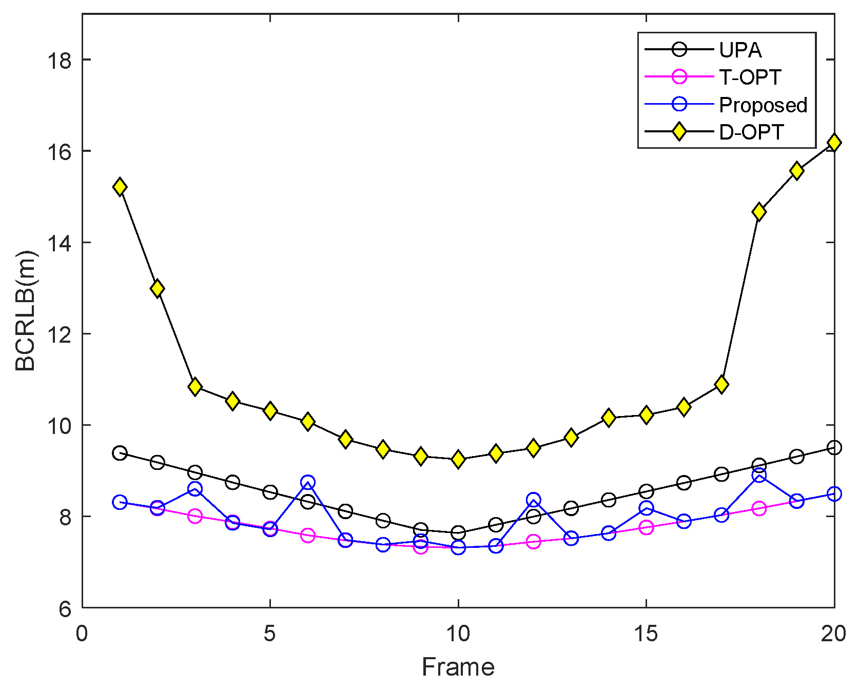
Figure 3 shows the BCRLB of the four algorithms. It can be seen that the performance of the proposed algorithm was close to that of T-OPT algorithm and lower than the BCRLB of the UPA algorithm, indicating that the algorithm demonstrated good tracking performance. In addition, the BCRLB of the D-OPT algorithm was the largest, indicating that its tracking performance was the worst.

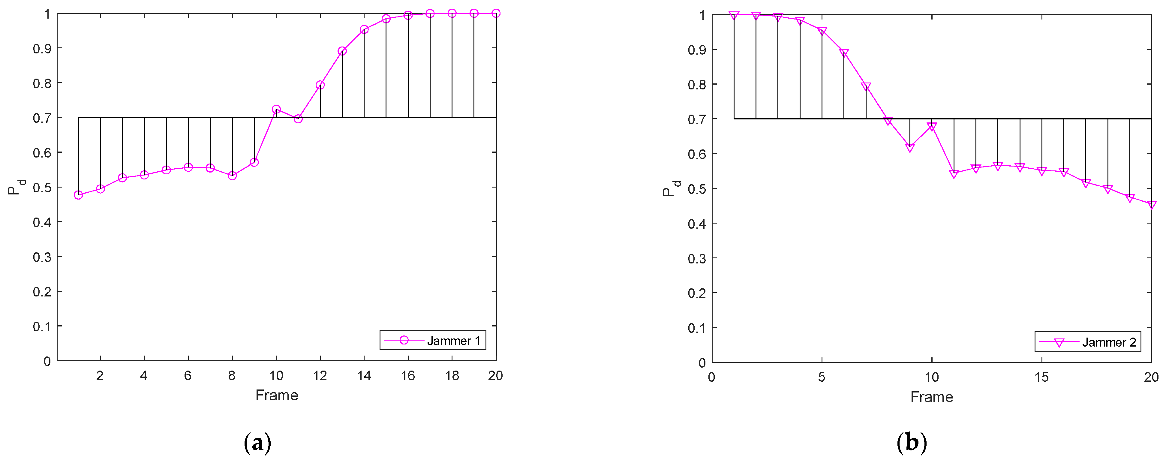
Figure 4, Figure 5, Figure 6 and Figure 7 show the detection performance of the four algorithms. The detection probability of the UPA algorithm was similar to that of the T-OPT algorithm; the detection of jammer 1 in the early stage was poor, and the detection of jammer 2 in the late stage was poor. The tracking of both jammers was seriously interrupted. The D-OPT algorithm focused on only the worst detection accuracy in relation to the jammers. The detection of the two jammers was relatively high throughout the whole process, and this shows that the radar network can improve the probability of detecting jammers through reasonable power allocation.

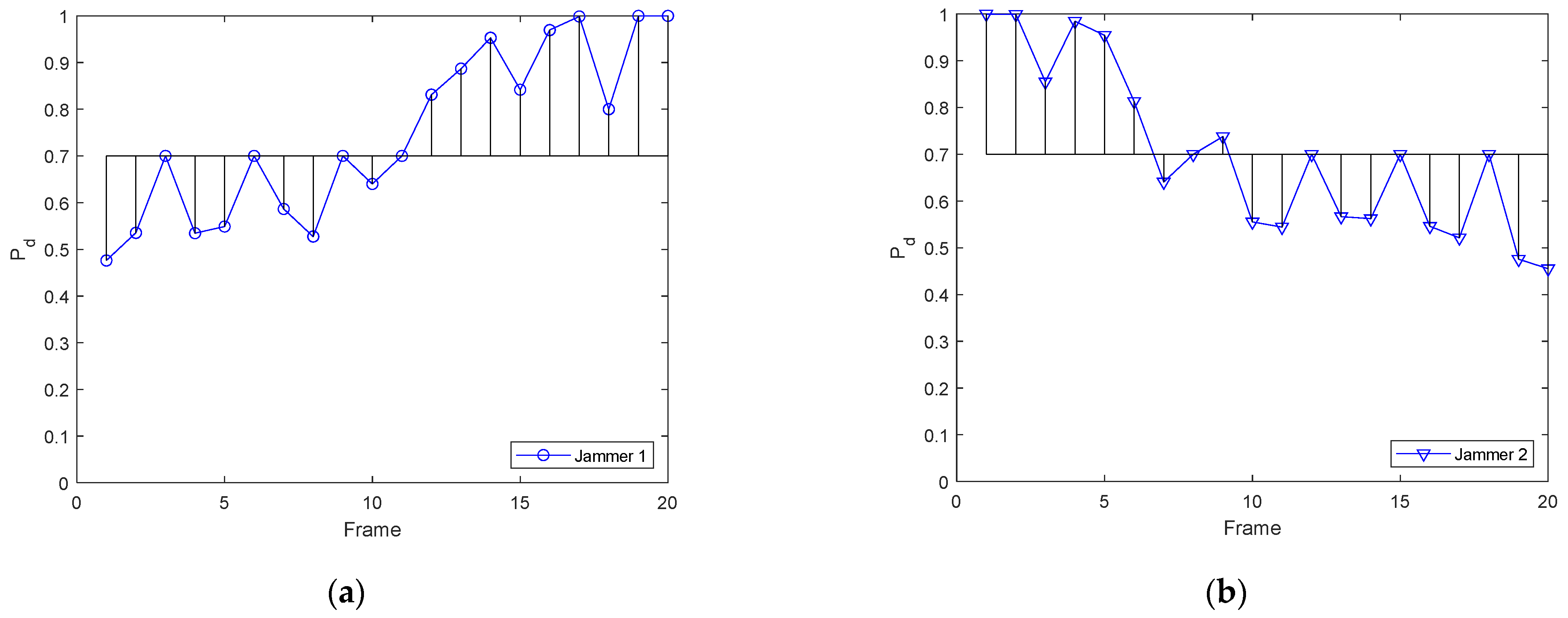
Figure 7 shows the detection performance of the proposed algorithm in relation to the two jammers. The detection of jammer 1 was poor in the early stage, and the detection of jammer 2 was poor in the later stage. Unlike the T-OPT algorithm, the probability of detecting jammer 1 in frames 3, 6, and 9 reached the detection threshold $P_d$, and the probability of detecting jammer 2 in frames 12, 15, and 18 reached the detection threshold $P_d$, avoiding interrupting the tracking of the jammers.

It can be seen from Figure 3, Figure 4, Figure 5, Figure 6 and Figure 7 that the BCRLB of the T-OPT algorithm was the smallest, but the tracking of the two jammers was seriously interrupted. The D-OPT algorithm had high detection accuracy, but the BCRLB was too large. Neither algorithm was conducive to the stable tracking of the jammers. On the basis of the T-OPT algorithm, through reasonable power allocation, the proposed algorithm was able to detect the jammers that were not tracked in multiple frames, with not only the smallest BCRLB, but also the ability to stably detect all jammers in multiple frames to ensure stable tracking of the jammers.

Figure 8a shows the power allocation results for the UPA algorithm; all radars used the same power to track the jammers. Figure 8b shows the power allocation results for the T-OPT algorithm. In the early stage of tracking, jammer 1 was far away, and radars 1 and 3 used more power to improve the tracking performance in relation to jammer 1. In the later stage of tracking, jammer 2 was far away, and radars 2 and 4 used more power to improve the tracking performance in relation to jammer 2. Figure 8c shows the power allocation results for the D-OPT algorithm. It can be seen that radar 2 used more power to improve the detection performance in relation to jammer 1 in the early stage of tracking, and radar 3 used more power to improve the detection performance in relation to jammer 2 in the later stage of tracking.

Figure 8d shows the power allocation results of the proposed algorithm. Unlike Figure 8b, jammer 1 was far away in the early stage of tracking and the probability of its detection was always low, so radar 2 used more power every two frames to improve the detection performance in relation to jammer 1, and this avoided interrupting the tracking of jammer 1. In the later stage of tracking, jammer 2 was far away and the probability of its detection was always low level, so radar 3 used more power every two frames to improve the detection performance in relation to jammer 2, and this avoided interrupting the tracking of jammer 2.

It can be seen from Figure 8 that the proposed algorithm combines the advantages of the T-OPT and D-OPT algorithms. On the one hand, it guarantees a small BCRLB on the basis of the T-OPT algorithm. On the other hand, we used the D-OPT algorithm to verify that the probability of detecting jammers could be improved by power allocation, which provided the basis for the tracking continuity.

5.2. Simulation Scenario 2

The second target reflectivity model was established according to this scenario. The time variation of the jammers in relation to radar 3 is depicted in Figure 9; the other RCSs stayed the same. Figure 10 shows the BCRLB of the four algorithms in this scenario. It can be seen that the proposed algorithm can still maintain good jammer tracking performance in the case of RCS fluctuation.

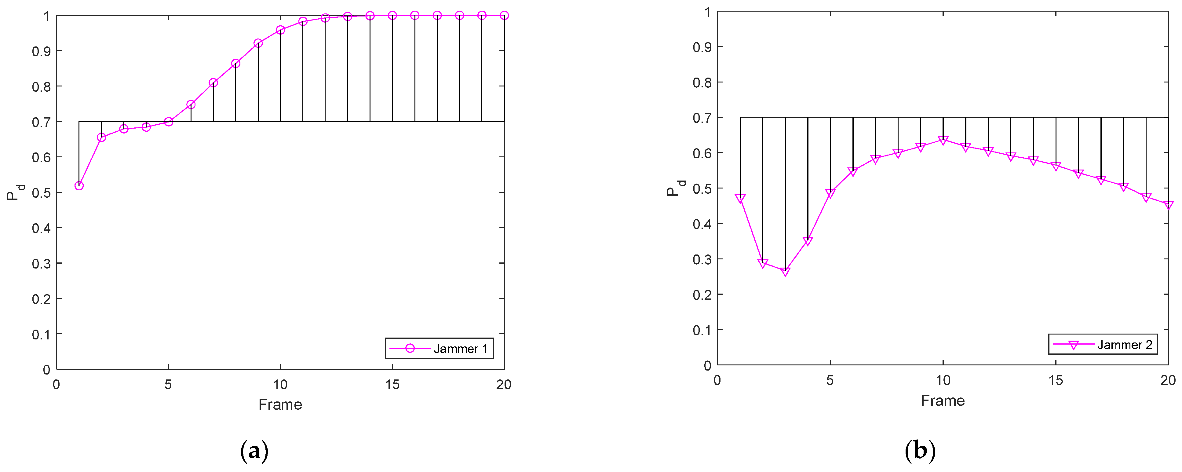
Figure 11, Figure 12, Figure 13 and Figure 14 show the detection performance of the four algorithms in the case of RCS fluctuation. The detection performance of the UPA algorithm for jammer 1 gradually increased, while the detection performance for jammer 2 gradually decreased as the frame increased. The detection performance of the T-OPT algorithm was similar to that of the UPA algorithm. In addition, the detection performance of the D-OPT algorithm was relatively high throughout the whole process.

Figure 14 shows the detection performance of the proposed algorithm for two jammers in the case of RCS fluctuation. As shown in Figure 14a, the detection accuracy in relation to jammer 1 was poor in the early stage, and the detection probability was improved by adjusting the power configuration every two frames. In addition, the detection probability in relation to jammer 1 in frame 3 reached the detection threshold $P_d$, so tracking interruption was avoided. As illustrated in Figure 14b, the detection accuracy in relation to jammer 2 remained at a low level, and the detection probability was improved by adjusting the power configuration every two frames. In addition, the detection probability in relation to jammer 2 in frames 3, 6, 9, 12, 15, and 18 reached the detection threshold $P_d$, which avoided tracking interruption.

It can be seen from Figure 10, Figure 11, Figure 12, Figure 13 and Figure 14 that the BCRLB of the T-OPT algorithm was the smallest, but the tracking of the two jammers was seriously interrupted, especially jammer 2. There were two reasons for this: on the one hand, the SINR changed due to the influence of jammer distance; on the other hand, the detection performance in relation to jammer 2 was always at a low level due to the small reflection coefficient of jammer 2 to radar 3. The D-OPT algorithm had high detection accuracy, but the BCRLB was too large. Neither algorithms was conducive to the stable tracking of the jammers.

On the basis of the T-OPT algorithm, the proposed algorithm was able to detect the jammers that were not tracked in multiple frames, especially jammer 2, through reasonable power allocation. The proposed algorithm not only had the small BCRLB, but was also able to stably detect all jammers in multiple frames to ensure stable tracking of the jammers.

Figure 15a shows the power allocation results of the UPA algorithm; all radars used the same power to track the jammers. Figure 15b shows the power allocation results of the T-OPT algorithm in the case of RCS fluctuation. Unlike Figure 8b, the power utilized by radar 3 remained at a low level for a long time. In the early stage of tracking, jammer 1 was far away, and radars 1 and 2 used more power to improve the tracking accuracy for jammer 1. At the later stage of tracking, jammer 2 was far away, and radars 2 and 4 used more power to improve the tracking accuracy for jammer 2.

Figure 15c shows the power allocation results of the D-OPT algorithm in the case of RCS fluctuation. It can be seen that radar 2 used more power to improve the detection performance in relation to jammer 1 in the early stage of tracking, and radar 4 used more power to improve the detection performance in relation to jammer 2 in the later stage of tracking. Unlike Figure 8c, the power of radar 3 remained at the lowest level.

Figure 15d shows the power allocation results of the proposed algorithm. Unlike Figure 8d, due to the influence of the reflection coefficient, the power of radar 3 remained at the lowest level. In addition, the detection probability in relation to jammer 2 was always low. Radar 4 used more power every two frames to improve the detection accuracy in relation to jammer 2, avoiding interrupting the tracking of jammer 2.

6. Conclusions

This paper proposes a multi-objective optimization algorithm to solve the jammer tracking problem of multi-static radar systems under suppression jamming. The echo signal model and measurement model of the multi-static radar are established, and the BCRLB is derived. A multi-objective optimization method is proposed, which uses the detection probability data for jammers in multiple frames, dynamically adjusts the weight coefficient, and reasonably allocates the radar power. It increases the probability of detecting jammers with less detection probability in multiple frames, and realizes the stable tracking of multiple jammers.