Abstract
Holographic synthetic aperture radar (HoloSAR) introduces a cutting-edge three-dimensional (3-D) imaging mode to the field of synthetic aperture radar (SAR), enriching the scattering information of targets by observing them across multiple spatial dimensions. However, independent phase errors among baselines, such as those caused by platform jitter and measurement inaccuracies, pose significant challenges to imaging quality. The phase gradient autofocus (PGA) method effectively estimates phase errors, but struggles to accurately estimate the linear component, causing vertical shift in HoloSAR subaperture imaging result. Therefore, this paper proposes a PGA-based phase error compensation method for HoloSAR to address the vertical shift issue caused by linear phase errors. This method can achieve phase error correction in both the echo domain and image domain with enhanced efficiency. Experimental results of simulated targets and real data from the GOTCHA system demonstrate the effectiveness and practicality of the proposed method.
1. Introduction
In the realm of synthetic aperture radar (SAR) [1,2,3,4,5,6,7,8] technology, the imaging capabilities are continuously expanding and evolving into multiple observational dimensions to capture comprehensive three-dimensional (3-D) scattering information of targets. Drawing inspiration from the concepts of circular SAR and tomographic SAR (TomoSAR), holographic SAR (HoloSAR) [9,10,11,12,13,14] emerges as a novel approach capable of extracting comprehensive target scattering characteristics leveraging on multiple baselines and azimuth angles. HoloSAR’s unique imaging mode overcomes the limitations of TomoSAR [15] regarding limited observational angles, while also addressing the height ambiguity and the challenge of extracting scattering information distribution along elevation faced by circular SAR [16] in single-baseline model.
Phase calibration stands out as a crucial technology for enhancing the 3-D imaging result of HoloSAR [17]. For the airborne SAR systems, acquiring two-dimensional (2-D) SAR images through repeated observations can introduce phase errors among baselines [18,19]. These errors are caused by factors such as aircraft position jitter, weather variations, and location error. Failure to compensate for these errors may result in blurred, distorted, or reduced-resolution tomographic reconstruction. Therefore, meticulous research into tomographic phase correction techniques is paramount for optimizing the imaging quality of HoloSAR.
One classic method is the persistent scatterer interferometric SAR (PS-InSAR) technique introduced by Ferretti et al. in 2001 [20]. The PS-InSAR method involves initially processing SAR images with a master image to extract deformation rates and residual phase information of PSs using analytical methods. This technology enables the estimation of atmospheric phase effects and phase variations caused by deformations during SAR tomographic imaging, allowing for error compensation. However, this method is complex in its implementation and exhibits limited applicability.
In recent years, various phase correction methods for multi-baseline airborne SAR data have been proposed. In [21], a method utilizing the “ALGAE” algebraic approach to separate ground reflections was introduced to achieve interferometric phase error compensation without the need for calibration targets. Despite its potential, the implementation of this method is hindered by its complex mathematical models and algorithms. In 2014, a two-step calibration method was introduced, incorporating a phase compensation function dependent on both range and azimuth directions [22]. The effectiveness of this method is heavily reliant on the initial phase value. In 2015, Tebaldini [23] presented the phase center double localization (PCDL) method, addressing vertical shift issues without requiring calibration targets or prior information. This method, however, necessitates a certain level of correlation among SAR images, making it less suitable in cases of low correlation. Most recently, in 2023, Wang [24] proposed a calibration method based on persistent scatterers (PSs), utilizing subspace decomposition and maximum interferometric spectral methods to extract multi-channel amplitude-phase inconsistency information at each PS. Subsequently, they fitted the variation curve and performed error compensation, tailoring this method specifically for large-scale scenarios.
Autofocus algorithms based on echo data error correction have always been a focal point in phase error correction research. One category involves sharpness optimization autofocus (SOA) methods. These methods use the sharpness of the imaging result as the objective function, the compensation phase as the independent variable, and the compensation phase corresponding to the maximum sharpness as the estimated value of the true phase error. Evaluation of sharpness typically employs criteria such as entropy and contrast [25]. In [26], a method involves minimizing the entropy of the inverted tomographic tomograms was proposed, but it suffers from vertical shift issues. To address this, a method based on phase derivative constrained optimization (PDCO) was proposed in [27], effectively resolving the problem. The advantage of this method is to calibrate the phase error pixel by pixel, and there is no need to make assumptions about the scene. Nonetheless, this method entails solving multi-dimensional optimization problems for each pixel, resulting in significant computational overhead. In 2020, an SOA method based on intensity square maximization was proposed in [28]. This method, compared to the PDCO method, achieves similar imaging quality but with higher efficiency.
Another category involves autofocus algorithms based on phase error functions, with the phase gradient autofocus (PGA) method being a representative example. The PGA method [29] directly estimates the phase error in the echo signal without establishing a phase error model. Theoretically, it can compensate for phase errors of any order, and is widely used in TomoSAR phase error compensation. In 2011, Sun [30] combined the least squares method and proposed an improved PGA phase error compensation method, estimating clutter variance based on the characteristics of clutter energy in prominent units. This method is more applicable, as it does not assume limitations on clutter. In 2019, Feng [31] applied the PGA method to correct phase errors among different channels in HoloSAR. It is important to note that the PGA method relies on the assumption of a slow spatial variation in the phase error, which is challenging to satisfy in large-scale scenarios. In 2021, Lu [32] proposed the network construction-PGA (NC-PGA) method to address this issue. This approach involves processing the imaging scene in blocks and applying the PGA method to estimate phase errors for each sub-block. Inspired by the concept of PS-InSAR, the method utilizes network construction (NC) to estimate the initial heights of prominent units, thereby eliminating the need for vertical shift estimation. In 2022, Lu [33] replaced NC with a block-structured network based on the NC-PGA method, using partially overlapping sub-blocks to reduce computational complexity. However, the accuracy of estimation in this method depends on the accurate estimation of initial scatterers.
In the context of HoloSAR, vertical shifts among different subapertures lead to non-co-planar imaging results during noncoherent addition, thereby causing a severe degradation in the final imaging quality. Existing research has not provided a satisfactory solution to this issue. For the first time, the vertical shift issue among HoloSAR subapertures is discussed in this paper, where an improved phase calibration method is developed. The advantages of the proposed method are as follows.
- Composite screening method for PSs: the combination selection method using the amplitude dispersion index (ADI) and ambiguity constraint yields more reliable PSs screening results.
- Improved PGA method: In the proposed beamforming (BF)-PGA method, multilook technology is employed to construct the covariance matrix by using the homogeneous pixels around PSs. This method can further enhance the noise robustness of the estimation, consequently reducing subaperture misalignment.
- Registration method based on projection images: the cumulative intensity projection registration (CIPR) method is introduced to achieve precise alignment of projection images of each subaperture, enhancing the quality of the final 3-D imaging result.
- Self-correction based on echo and image domains: The proposed methods, BF-PGA and CIPR, represent self-correction approaches based on echo data and imaging results, respectively. These methods eliminate the need for manual deployment of calibration targets and can be implemented using a single polarization channel.
This paper is organized as follows. In Section 2, HoloSAR imaging model and problem formulation are presented. Section 3 clarifies the principle and implementation of the proposed method. The effectiveness and practicability of the proposed algorithm are validated in Section 4 by using simulated data and real data. Then, in Section 5, the principle and applicability of the CIPR method are discussed, and an analysis is conducted on the computational complexity of the proposed method. Finally, conclusions are drawn in Section 6.
2. HoloSAR Model and Problem Formulation
The geometry model of HoloSAR is illustrated in Figure 1. The directions of the azimuth, ground range, and height are represented by x, y, and z, respectively. r denotes the slant range, while s represents the elevation direction. The airborne platform moves in a circular motion around the imaging area, with M different baseline heights. Due to the anisotropic scattering characteristics of the targets, it is not feasible to coherently image the entire azimuthal aperture ( = 360°). Therefore, this paper divides the complete aperture into Q subapertures with equal angles and no overlap, and each subaperture is processed separately. For each subaperture, a total of M single look complex (SLC) images of the area of interest are obtained from M different tracks.
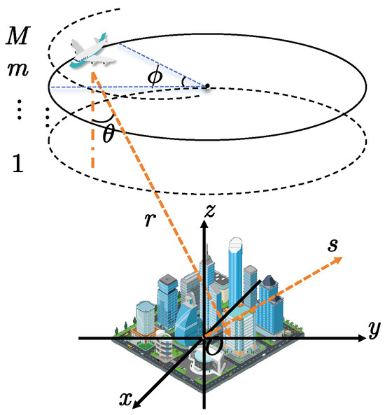
Figure 1.
Geometry model of HoloSAR imaging.
After pre-processing steps such as image registration, deramping, and phase calibration, each complex pixel in the mth SLC image is given as
where is the complex scattering coefficient along elevation s. is the spatial wavenumber along elevation, depending on elevation aperture position between the mth SLC image and the reference image. donates the carrier wavelength of radar, and is the reference slant range between target and platform.
It can be inferred from Equation (1) that the mth pre-processed SLC image can be seen as the Fourier transform of the complex scattering coefficients in elevation direction. As a result, the height and reflectivity of scatterers can be determined by identifying the peaks in the frequency domain. The discretization of Equation (1) with respect to elevation s can be expressed as
where is the dimensional measurement vector with complex value, is the dimensional steering matrix, is the dimensional discrete reflectivity vector, and is the dimensional noise vector. These vectors can be represented as
where describes the transpose operator. The imaging results of each subaperture are inherently tied to their respective imaging coordinate systems, due to varying viewing angles. To consolidate these diverse results effectively, a process of coordinate projection is implemented. This transformation aligns the imaging result of each subaperture into the common ground coordinate system, facilitating seamless integration and summation for comprehensive analysis. The transformation formula is given as
where represents the central azimuth angle of the qth subaperture, represents the position of the object under the qth subaperture imaging coordinate, indicates the position of the same object under the common coordinate system used for noncoherent addition, while signifies the average radar incidence angle.
Restatement of the Problem
The echo data considered in this paper are obtained from airborne repeat-pass case, which leads to temporal decorrelation among baselines. Additionally, errors in baseline estimation resulting from aircraft position deviations also contribute to phase disturbances. These factors ultimately introduce additional phase error terms to the complex values of the mth SLC image. As a consequence, these errors lead to blurred, distorted, and reduced resolution in the estimation results of tomographic tomograms. In light of the phase error influence, (1) is restated as
where the phase error term is a simplified form of . The purpose of this paper is to estimate and compensate this phase error, ultimately improving the quality of the HoloSAR imaging result.
3. Proposed Phase Calibration Method
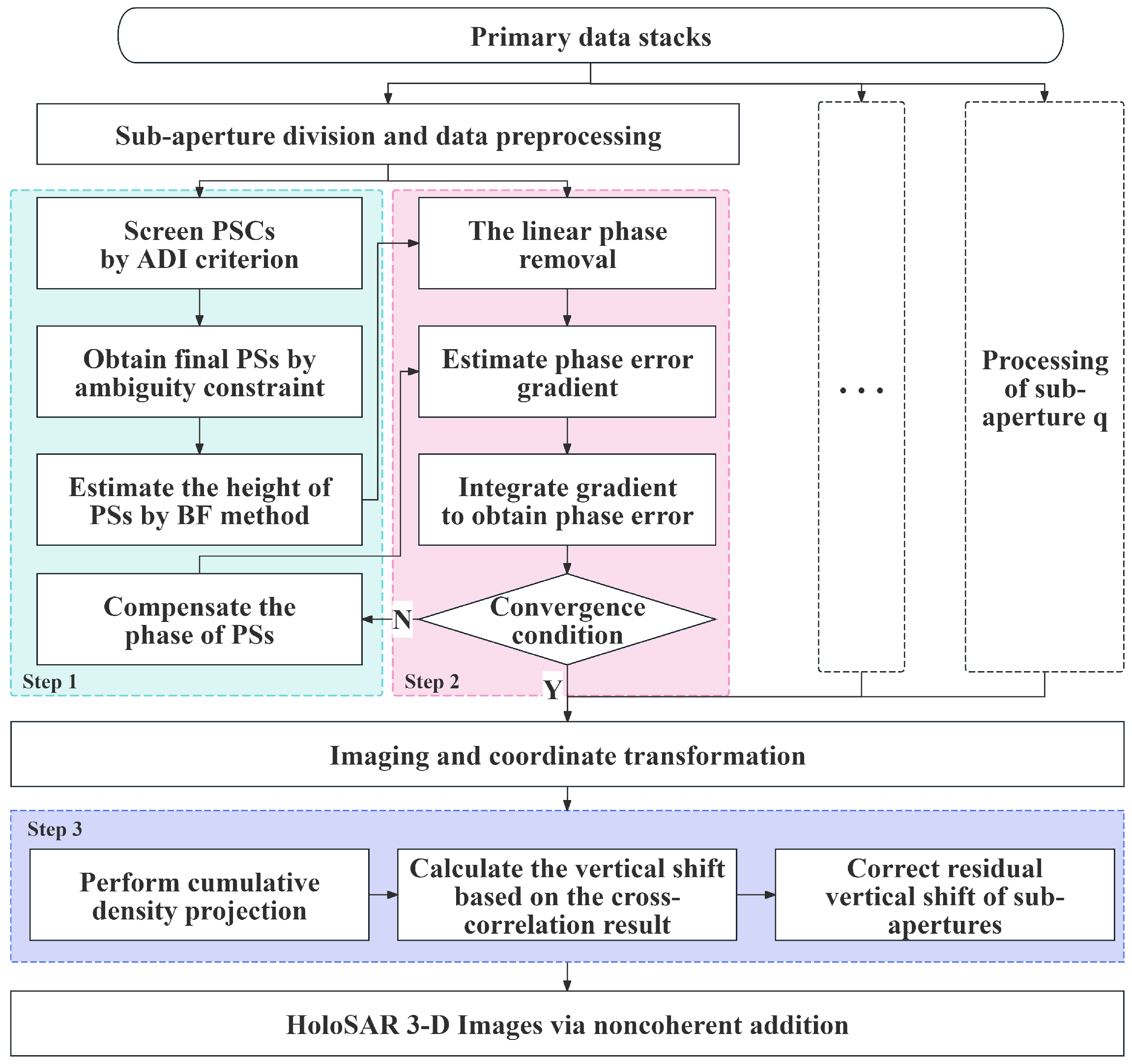
This section introduces the principle and implementation of the proposed method in detail. The proposed method can be delineated into three distinct steps:
- Selection of PSs and initial height estimation using the BF method.
- Phase error estimation through the PGA method.
- Subsequent alignment of the subaperture imaging results utilizing the CIPR method.
3.1. PS Selection Principle
In this step, the persistent scatterer candidates (PSCs) containing only one strong scatterer are selected from the set of SLC images first. The ADI method is first employed, which is defined as
This method evaluates the amplitude variation of pixels under different baselines, and the smaller is, the more stable the amplitude characteristic of the selected pixel. When falls below the preset threshold, the pixel is marked as PS. However, the ADI method only considers the stability of PSCs without factoring in scattering intensity, potentially leading to misjudgments or missed judgments based solely on this criterion.
Building upon the previous step, this paper introduces the ambiguity constraint method to further screen PSCs with a reliable estimation result. The ambiguity is defined as the power ratio between the highest sidelobe and the main lobe. When the ambiguity is greater than the set threshold, the corresponding PSC is unreliable. This composite threshold method combines the “strong” and “stable” characteristics of PSs, resulting in a more effective and reliable selection compared to the single-threshold method.
Through the above steps, PSs are preliminarily determined from PSCs. The data of the kth PSs in the mth SLC image can be expressed as
where and are the scattering coefficients of the kth idiosyncratic point and the layer tomography direction towards the height, respectively. is the clutter composed of other weak scatterers and noise, which can be modeled as an independent identically distributed Gaussian white noise with a mean of zero during the imaging process.
3.2. The Implement of the PGA Method in HoloSAR
The PGA method assumes phase error is stable within ten to one hundred meters, varying slowly and depending on the scenario [19,34]. In this paper, the maximum likelihood estimation (MLE) method is used to estimate the phase error gradients. Under the modeling of the MLE method, estimation of the phase error gradient is defined as
where is the estimated value of the gradient of phase , and is the phase extraction operator. The estimation of phase errors can be derived based on , i.e.,
In HoloSAR, only the amplitude of the target scattering coefficient is utilized, disregarding the phase difference between the true value and . It is worth noting that an approximation is employed while deriving . Since the approximation condition is not necessarily satisfied at the beginning, iteration is necessary to optimize the estimation result gradually. The termination condition is often set as the difference between two consecutive estimates falling below a specified threshold,
where and are the results of phase error estimation in two adjacent two iteration. The threshold value is typically set to 0.001 [32].
3.3. Removal of Linear Phase by BF Method
3.3.1. Cause of Linear Phase
The derivation process in Section 3.2 is based on the assumption that all PSs lie on the plane defined by , which is usually impractical. The case of a single scattering element of height was first considered. Without removing the linear phase term corresponding to the height at , the final phase term obtained by the gradient summation is estimated as
According to the Fourier transform principles, the additional phase term in Equation (11) induces vertical shift in the imaging result. After comprehensive influence of PSs, the phase error is reformulated as
where the m ranges from 2 to M.
3.3.2. The Beamforming Method
According to the above analysis, the linear phase error can be better avoided only by accurate estimation of . The BF algorithm is a classic nonparametric method for estimating direction of arrival in array signal processing. Its notable features include high efficiency and robustness against noise. In this paper, the BF method is used to the inversion of the tomographic profiles with the specific expression
where is the dimensional sample covariance matrix calculated by the spatial average over independent homogeneous adjacent pixels, and the robustness of the estimation results can be improved by the multi-look approach. is the dimensional steering vector corresponding to the elevation sample s. After removing the linear phase error corresponding to each PS, the vertical shift is better suppressed. However, there is a deviation between the estimated and true height, leading to a residual vertical shift that requires further correction.
3.4. Secondary Calibration by the CIPR Method
In this section, the CIPR method is proposed to further align the preliminary 3-D imaging result of each subaperture compensated by BF-PGA.
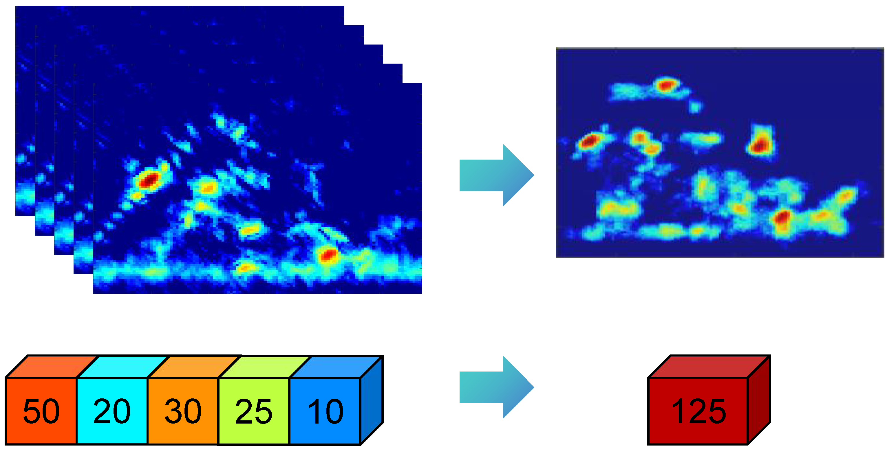
Generally, the 3-D imaging result is projected to 2-D plane in order to observe the structure of the target and the distribution of the scattering intensity. The cumulative intensity projection is a method for projecting 3-D data onto a 2-D image plane by accumulating values along a specified axis, which can reflect the internal structure information more clearly, as shown in Figure 2.
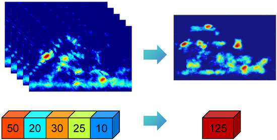
Figure 2.
Schematic diagram of cumulative intensity projection.
The core idea of the CIPR method is to reduce the dimensionality of 3-D data to 2-D using cumulative intensity projection. By registering the projection images of each subaperture, it indirectly calculates the vertical shift among subapertures, thereby estimating the overall residual linear phase error. The registration step is realized by calculating the cross-correlation of images and finding the position corresponding to the local maximum. For a fixed pixel , the cross-correlation is given as
where is main image and is the secondary images. Based on the peak position of cross-correlation, the relative offset among subapertures can be determined, facilitating the alignment of 3-D imaging results onto the same elevation plane.
The overall flow of the proposed method is given in Figure 3. After phase calibration, the final 3-D imaging result is obtained by noncoherent addition.

Figure 3.
Schematic diagram of the proposed method.
4. Experimental Results and Analysis
The effectiveness and practicability of the proposed method are proved through simulated and real data experiments in this section. To comprehensively assess the performance of the proposed method, it is compared against widely utilized techniques in phase calibration: minimum entropy autofocus (MEA), contrast optimization autofocus (COA), PGA, and the state-of-the-art NC-PGA method. These methods have been extensively applied in the field and their effectiveness has been established.
4.1. Experiments on Simulated Data
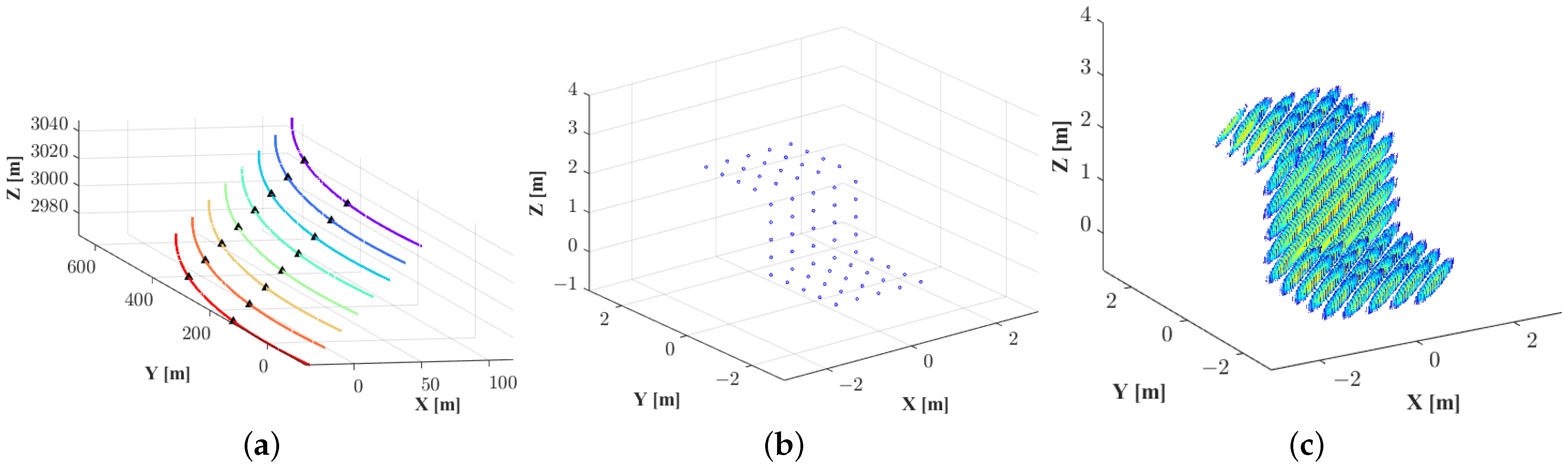
The simulation parameters for center frequency and bandwidth are set at 9.6 GHz and 640 MHz, respectively. The simulation scenario and target are shown in Figure 4. In the simulation experiment, the SAR data stacks from eight passes were generated across three consecutive sub-apertures, with a total baseline length of 140 m evenly distributed along the elevation (as shown in Figure 4a). The azimuth angle of each sub-aperture relative to the scene center ranges from 5 degrees. In Figure 4a, arcs of various colors represent different tracks, and black triangles indicate the boundaries among sub-apertures. The theoretical azimuth resolution is 0.22 m, the slant range resolution is 0.23 m, the resolution along elevation is 0.96 m, and the unambiguous height is 6.67 m. The scatterers that constitute the simulated target have a scattering coefficient of 1, with the highest scatterers at 2 m and the lowest scatterers at 0 m. The specific distribution of the scatterers and the imaging result without phase error are shown in Figure 4b and Figure 4c, respectively.
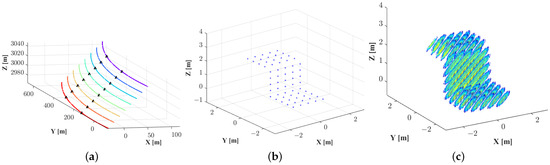
Figure 4.
Diagram of simulation scene. (a) Distribution of baselines; (b) simulated target; (c) ideal imaging result.
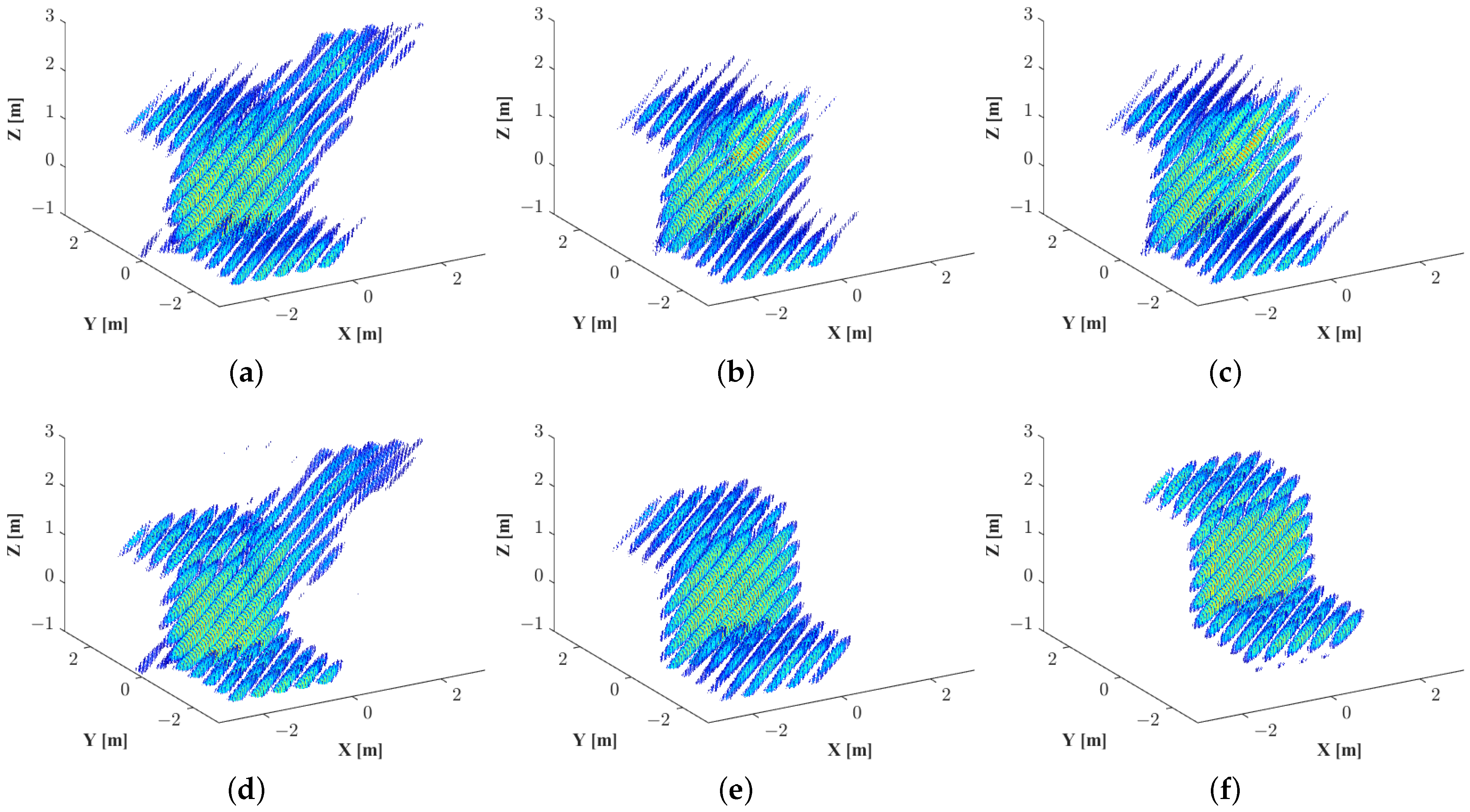
Phase errors distributed randomly within the range of radians along the elevation are added to the registered and deramped SLC images. Given the scale of the imaging scene and the spatial relationship between the scene and the radar, it is assumed that the phase error remains constant across the entire imaging area. Therefore, each SLC data only requires multiplication by the same phase error term. The 3-D imaging results after phase calibration by different methods are presented in Figure 5. The presence of phase errors results in blurred imaging result, hindering the clear interpretation of the target information (see Figure 5a). After phase error correction, the target exhibits improved focusing results with clear outlines. Both the MEA and COA methods produce similar imaging results, but they both show blurring at the vertical plane of the reconstructed target due to the presence of layover in the profile (see Figure 5b,c). The PGA and NC-PGA methods exhibit significant vertical shifts (see Figure 5d,e). In Figure 5d, the effect of PGA method on phase error correction is not obvious compared with the imaging results with phase errors. While the NC-PGA method yields a generally clear imaging result, noticeable broadening of the main lobe is evident (see Figure 5e). By contrast, the proposed method achieves the most similar inversion result with error-free one.
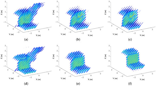
Figure 5.
Comparison of simulated imaging results. (a) The data with phase error; the data after phase error compensation by using the (b) MEA, (c) COA, (d) PGA, (e) NC-PGA, and (f) the proposed method, respectively.
4.2. Experiments on Real Data
4.2.1. Data Introduction
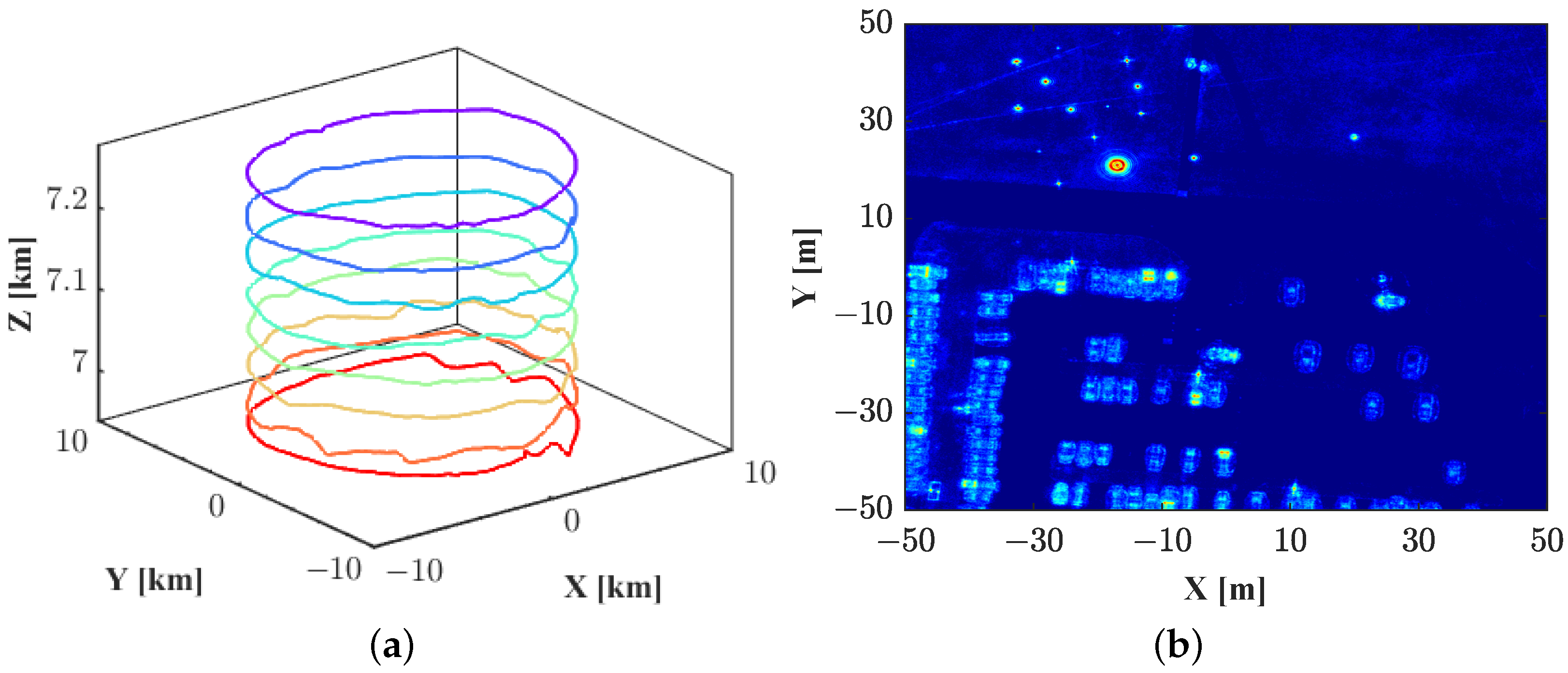
In 2006, the Air Force Research Lab (AFRL) conducted field flight tests of airborne HoloSAR, collecting eight sets of fully polarized X-band CSAR data with different altitude baselines [35,36,37]. The central frequency was 9.6 GHz, with a bandwidth of 640 MHz, and the incident angle ranged from 43.7° to 45°. The imaging scene was a parking lot of m, which included a large number of civilian vehicles and calibration targets. Figure 6 depicts the basic situation of this test. In Figure 6a, the flight trajectories of the eight passes are displayed. The amplitude image obtained through the noncoherent addition of the 2-D imaging results from multiple subapertures is depicted in Figure 6b. These data were made publicly available for scholars worldwide to download in 2008, serving as support for high-resolution 2-D and 3-D imaging studies [38].
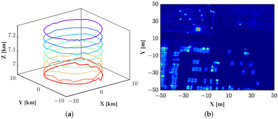
Figure 6.
Data of the experimental area. (a) Flight paths. (b) VV channel data of the selected area.
In this paper, the complete 360° azimuthal aperture is divided into every 5° subaperture without overlap. Each subaperture contains data of eight tracks in VV polarization. Phase error compensation and imaging of each subaperture are independent of each other. The specified target for imaging is a tractor, with its optical image shown in Figure 7. The length and width of the tractor are 4.73 m and 3.07 m, respectively.
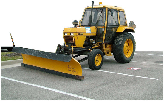
Figure 7.
Optical image of tractor.
4.2.2. The PSs Selection Processing
Under each subaperture, the back projection (BP) algorithm is employed to obtain 2-D SLC images. Subsequently, the registration and deramping are performed. Following the composite threshold method depicted in Section 3.1, PSs are selected from PSCs. The selection outcomes of the whole imaging scene are illustrated in Figure 8.
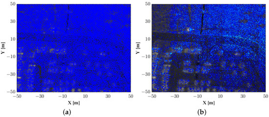
Figure 8.
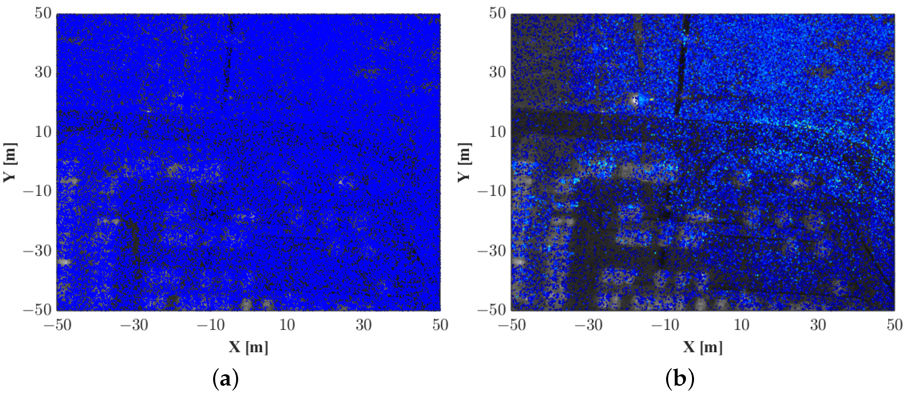
Selection results of PSs by different methods. (a) The ADI method. (b) The composite threshold method.
Based on the research of [39], the ADI threshold is determined to be 0.23. Additionally, the ambiguity threshold is established at 0.5. When only the ADI method is used, 246,499 PSs in the scene are selected (see Figure 8a). However, after applying the composite threshold method, a total of 181,868 PSs are identified (see Figure 8b). The higher the brightness of PSs in Figure 8b, the lower the ambiguity, and the more reliable the corresponding inversion results. In summary, the PSs screened through the composite threshold method more closely align with the distribution characteristics of scene targets, mainly concentrating in areas of strong scattering. This method can yield higher-quality PSs, laying the groundwork for subsequent phase calibration efforts.
4.2.3. Primary Phase Error Correction
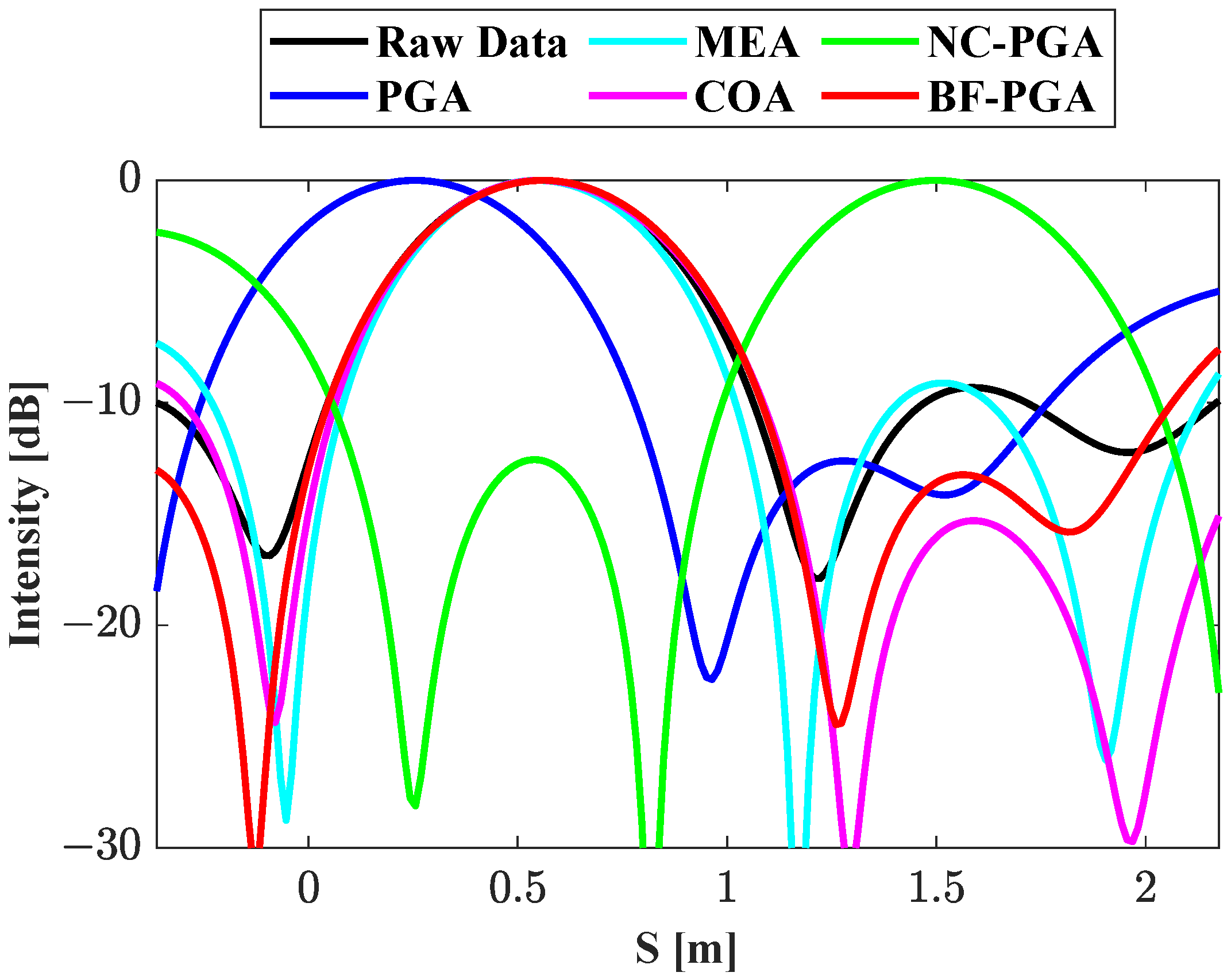
After selecting the PSs, the robust BF method is employed to estimate elevations of PSs. In this paper, an estimation window with the central pixel being the PS and a radius of 6 pixels was utilized to estimate the sample covariance matrix. Figure 9 illustrates one of the inversion tomograms of a selected PS. The black line in Figure 9 represents the inversion profile without phase error correction. It can be observed that most phase error correction methods are effective in suppressing sidelobes in the estimation results. However, the inversion results of the PGA and NC-PGA methods exhibit significant shifts, and the NC-PGA method even generates higher sidelobes than raw data. This indicates that the compensating phase obtained based on the assumption that the phase error is spatially invariant cannot guarantee a good compensation effect for every pixel.

Figure 9.
Inversion profiles of the selected pixel along elevation.
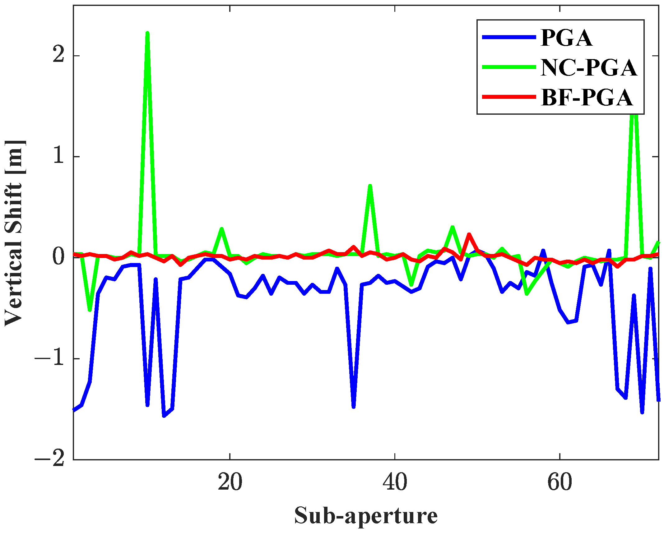
Figure 10 illustrates the vertical shifts of various subapertures relative to the reference after phase calibration by different PGA-based methods. The variances of vertical shift of PGA, NC-PGA, and the proposed method are 0.222, 0.134, and 0.020, respectively. It is evident from the graph that the PGA method exhibits the highest variance in vertical shift across subapertures, indicating highly unstable estimation results. Even after correction using the NC method, significant shifts still occur in some subapertures. The accuracy of the NC method is heavily reliant on the reference scatterer estimation. Bias in the elevation of reference scatterer can lead to cumulative height errors in PSs, as noted in [40]. In comparison to these two methods, the proposed BF-PGA method provides more accurate height estimates for PSs, thus better mitigating vertical shifts induced by linear phase errors.
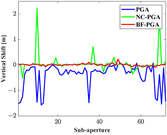
Figure 10.
The vertical shift of each subaperture.
4.2.4. Error Correction in Image Domain
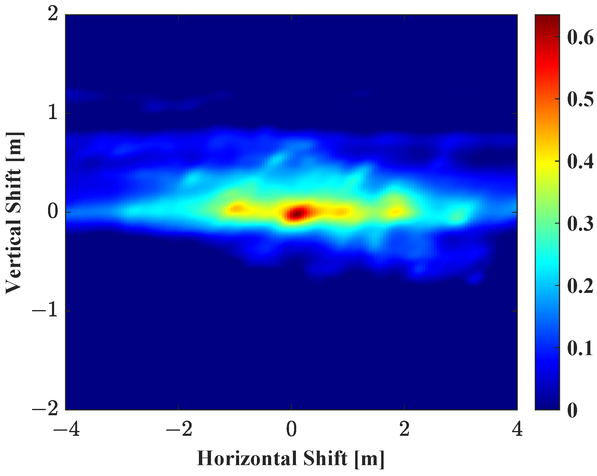
To compensate for the residual phase error among subapertures, the CIPR method proposed in Section 3.4 is employed. In this paper, the X-Z plane is selected as the projection plane because it contains abundant structural information about the target. Figure 11 illustrates the cross-correlation results between the second and first subaperture projection image in the X-Z plane, using 3-D imaging results compensated by the BF-PGA method. The coordinate of the maximum value in the 2-D cross-correlation matrix represent the shift of the image relative to the reference image. Based on the transformation relation in (4), the vertical shift can be corrected by adjusting the entire imaging result. The chain registration rule is employed to correct vertical shift subaperture by subaperture, which involves treating the current subaperture projection as the slave image and the projection of the previous subaperture as the master image.

Figure 11.
The 2-D cross-correlation matrix.
4.2.5. 3-D Imaging Result Analysis
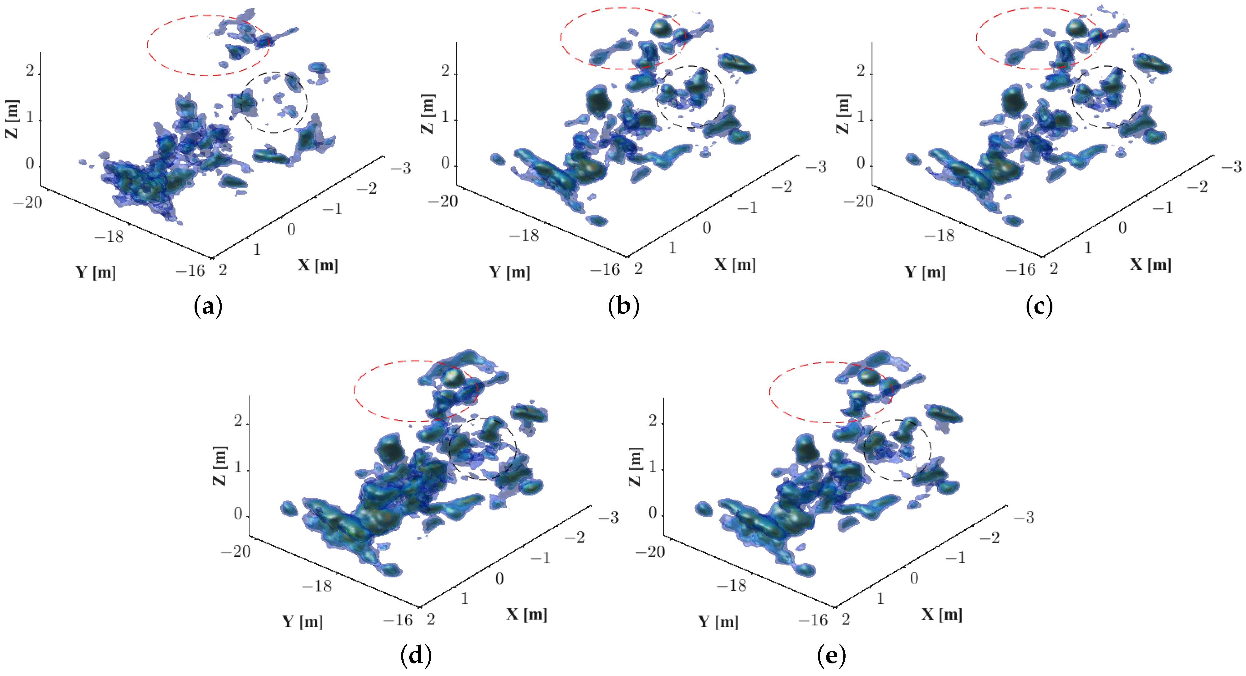
After noncoherent addition of the 3-D volume data of each subaperture, the holographic 3-D target images depicted in Figure 12 are obtained. Figure 12 utilizes a layered rendering technique to exhibit the surface of the imaging results within the intensity range of −25 dB to −15 dB. Additionally, Figure 13 illustrates the projection images across distinct planes.
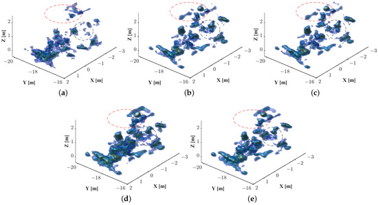
Figure 12.
The 3-D imaging results of tractor after phase error compensation by using the (a) PGA, (b) MEA, (c) COA, (d) NC-PGA, and (e) the proposed method, respectively.
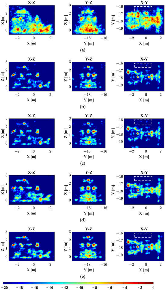
Figure 13.
Projection of imaging results on different planes. (a) PGA, (b) MEA, (c) COA, (d) NC-PGA, and (e) the proposed method, respectively. The images on the left, middle, and right correspond to the projection results along the X-Z, Y-X, and X-Y axes, respectively.
The imaging results of the PGA method are the poorest, as evidenced by the least reflected target structural information in the 3-D result (see Figure 12a) and severe blurring in the projected image (see Figure 13a). Both the MEA and COA methods show similar imaging results, with partial missing restoration of the top of the tractor and the presence of false targets within the imaging range (see red circles in Figure 12b,c). In Figure 12e, not only is the structure information of the tractor relatively complete, but the outliers in the black circle are also much less than those in other methods. From the white rectangle in Figure 13, noticeable outliers are apparent around the tractor imaging results obtained by the PGA, MEA, and COA methods. In contrast, the imaging results achieved with NC-PGA and the proposed method demonstrate clearer results. In order to evaluate the imaging quality more comprehensively, Table 1 compares the entropy and contrast values of different methods across the X-Z plane, Y-Z plane, X-Y plane, and 3-D images.

Table 1.
Comparison of image quality evaluation metrics.
The definition of image entropy is [41]
where is the intensity probability density of the selected pixel magnitude in the 3-D image. is donated as
where is the intensity of pixel. , , and are the size of 3-D image. The definition of image contrast is defined as
where represents the expectancy factor.
Observing Table 1, it is clear that the proposed method consistently achieves the lowest entropy values across all planes and the 3-D image. Its contrast levels are just below those of MEA and COA on the planes, but it ranks the highest in the 3-D image. Overall, the proposed method demonstrates superior performance compared to other methods, yielding clearer inversion results and less outliers.
5. Discussion
5.1. Principle and Applicability of CIPR in HoloSAR
In urban environments, the artificial targets are often anisotropic, exhibiting varying scattering characteristics at different observation angles. This anisotropy leads to distinct projection features for targets at different angles, thereby impacting the effectiveness of the CIPR method in registration. Therefore, it is crucial to establish registration criteria that are suitable for anisotropic targets. A related study [42] demonstrated that the strong scattering properties of the edges and angles of artificial objects tend to remain relatively stable within the rotation angular range of 10° to 20°. This implies that the imaging results and projections of each subaperture in this angular range exhibit similar structural characteristics.
In consideration of this feature, this paper employs a chain registration rule, using the current subaperture projection as the secondary image and the previous subaperture projection as the primary image. This approach guarantees that the two images exhibit similar target features during registration. Additionally, it is scalable to accommodate more subaperture projections, maintaining consistent target features to achieve precise registration.
The proposed CIPR method is a phase correction technique based on image domain, which can be integrated with any HoloSAR imaging method. It is important to note that the CIPR method performs optimally in small-scale scenarios, particularly when dealing with single targets. When multiple targets are present in the scene and their 2-D projections cannot be fully separated in any direction, there arises a situation where the scattering information of these targets overlaps in the projection image. As a result, the registration quality may decrease due to the complexity added by overlapped scattering information, thereby reducing the accuracy and robustness of the algorithm.
5.2. Computational Complexity Analysis
This section analyzes the computational complexity of the proposed method compared to MEA, COA, and NC-PGA methods.
5.2.1. The MEA and COA Methods
Ideally, the distribution peak of the target scattering coefficient along elevation is formed by the combination of several Dirichlet functions at the target positions. Influenced by phase errors, the imaging results can suffer from higher sidelobes, blurring, and reduced resolution, all of which can lead to a reduction in the sharpness of the inversion results. Overall, better focused imaging results are characterized by higher sharpness. It is therefore desirable to maximize the sharpness of the inversion results
where is the phase vector to be compensated for in the SLC images, is the backscatter intensity of the target at the elevation , and is the sharpness cost function. The MEA and COA methods use entropy and contrast, respectively, as criteria to evaluate the sharpness of inversion profiles. The solution space for Equation (18) is of dimension M. Since these methods do not rely on the phase error invariant assumption, each pixel requires M-dimensional numerical search to find the optimal solution, which results in significant computational burden.
5.2.2. The NC-PGA and Proposed BF-PGA Methods
One of the main differences between the proposed BF-PGA and NC-PGA lies in the method used to estimate the elevations of PSs, which also accounts for the disparity in computational load. Assuming a total of P PSs are selected, and a maximum network of U arcs is constructed, the NC-PGA method employs a least squares estimator to estimate the elevations of the selected PSs, which can be represented as
where is a dimensional vector representing the absolute heights of PSs, is a dimensional vector representing the relative heights of arcs calculated based on the Delaunay triangulation network, and is a dimensional diagonal weighted matrix. is a dimensional coefficient matrix reflecting the connectivity of PSs, i.e.,
where and 1 represent the end points and start points of the arcs, and each row contains only one start point and one end point, with all other elements being 0. The computational complexity of the NC-PGA method based on least squares can be expressed as
For the same number of PSs, the spectral estimation method BF requires spatial spectrum search by using Equation (13), with a computational complexity of
where L represents the number of samples along elevation. By comparison, it is evident that the complexity of the proposed method is linear with respect to P, the number of PSs, while the NC-PGA method has a cubic complexity. As the number of PSs increases, the advantages of the proposed method become more pronounced.
In the same computing environment, we use AMD Ryzen 7 5800h with Radeon graphics processor, running at 3.20 GHz. These components are sourced from Lenovo, based in Beijing, China. Equation (22) only takes 0.057 s to compute, while Equation (21) requires 0.266 s. In comparison, the MEA and COA method take considerably longer, with respective times of 254.766 s and 301.179 s. The efficiency of the proposed algorithm is 4.67 times that of NC-PGA method, far exceeding that of MEA and COA methods.
6. Conclusions
This paper proposes a phase calibration method for addressing the issue of vertical shift in HoloSAR subaperture. Initially, the proposed BF-PGA method employs the BF approach to estimate and compensate for the elevation phase of PSs, followed by the use of the PGA method to estimate the phase error term. The BF-PGA method effectively avoids introducing linear phase errors in PGA. Subsequently, the proposed CIPR method is used to estimate residual vertical shift by calculating cross-correlation of cumulative intensity projection images.
To validate the effectiveness of the proposed method, this paper conducts a comparative analysis with four existing mainstream phase error correction methods, performing a qualitative assessment of their imaging results on simulated data. Furthermore, the tractor from the GOTCHA dataset is chosen as the imaging target, allowing for a quantitative evaluation of the imaging results using metrics such as entropy and contrast. The findings indicate that the proposed method not only achieves higher computational efficiency but also yields clearer 3-D imaging results compared to the other methods.
Author Contributions
Conceptualization, F.H. and D.F.; formal analysis, F.H.; funding acquisition, F.H. and D.F.; investigation, F.H. and D.F.; methodology, F.H. and D.F.; resources, D.F. and X.H.; supervision, D.F., S.G., Y.H. and X.H.; validation, F.H. and J.H.; writing—review and editing, F.H. and J.H. All authors have read and agreed to the published version of the manuscript.
Funding
This work was supported in part by the National Natural Science Foundation of China under Grant 62101562.
Data Availability Statement
Restrictions apply to the availability of these data. Data were obtained from AFRL and are available at https://www.sdms.afrl.af.mil/main.php, accessed on 17 June 2024, with the permission of AFRL.
Conflicts of Interest
The authors declare no conflicts of interest.
References
- Brown, W.M.; Porcello, L.J. An introduction to synthetic-aperture radar. IEEE Spectr. 1969, 6, 52–62. [Google Scholar] [CrossRef]
- Wiley, C.A. Synthetic aperture radars. IEEE Trans. Aerosp. Electron. Syst. 1985, AES-21, 440–443. [Google Scholar] [CrossRef]
- Song, S.; Dai, Y.; Jin, T.; Wang, X.; Hua, Y.; Zhou, X. An Effective Image Reconstruction Enhancement Method with Convolutional Reweighting for Near-field SAR. In IEEE Antennas and Wireless Propagation Letters; IEEE: Piscataway, NJ, USA, 2024. [Google Scholar]
- Ge, S.; Feng, D.; Song, S.; Wang, J.; Huang, X. Sparse Logistic Regression Based One-Bit SAR Imaging. IEEE Trans. Geosci. Remote Sens. 2023, 61, 3322554. [Google Scholar] [CrossRef]
- Xie, Z.; Xu, Z.; Fan, C.; Han, S.; Huang, X. Robust radar waveform optimization under target interpulse fluctuation and practical constraints via sequential lagrange dual approximation. IEEE Trans. Aerosp. Electron. Syst. 2023, 59, 9711–9721. [Google Scholar] [CrossRef]
- Ge, S.; Song, S.; Feng, D.; Wang, J.; Chen, L.; Zhu, J.; Huang, X. Efficient near-field millimeter-wave sparse imaging technique utilizing one-bit measurements. IEEE Trans. Microw. Theory Tech. 2024; Early Access. [Google Scholar]
- Xie, Z.; Wu, L.; Zhu, J.; Lops, M.; Huang, X.; Shankar, B. RIS-Aided Radar for Target Detection: Clutter Region Analysis and Joint Active-Passive Design. IEEE Trans. Signal Process. 2024, 72, 1706–1723. [Google Scholar] [CrossRef]
- Song, S.; Dai, Y.; Sun, S.; Jin, T. Efficient Image Reconstruction Methods Based on Structured Sparsity for Short-Range Radar. IEEE Trans. Geosci. Remote Sens. 2024, 62, 5212615. [Google Scholar] [CrossRef]
- Ponce, O.; Prats-Iraola, P.; Scheiber, R.; Reigber, A.; Moreira, A.; Aguilera, E. Polarimetric 3-D reconstruction from multicircular SAR at P-band. IEEE Geosci. Remote Sens. Lett. 2013, 11, 803–807. [Google Scholar] [CrossRef]
- Ferrara, M.; Jackson, J.A.; Austin, C. Enhancement of multi-pass 3D circular SAR images using sparse reconstruction techniques. In Proceedings of the Algorithms for Synthetic Aperture Radar Imagery XVI, Online, 12–16 April 2009; Volume 7337, pp. 9–18. [Google Scholar]
- Ponce, O.; Prats, P.; Scheiber, R.; Reigber, A.; Moreira, A. Study of the 3-D impulse response function of holographic SAR tomography with multicircular acquisitions. In Proceedings of the EUSAR 2014; 10th European Conference on Synthetic Aperture Radar, Berlin, Germany, 3–5 June 2014; pp. 1–4. [Google Scholar]
- Moses, R.L.; Potter, L.C. Noncoherent 2D and 3D SAR reconstruction from wide-angle measurements. In Proceedings of the 13th Annual Adaptive Sensor Array Processing Workshop, MIT Lincoln Laboratory, Lexington, MA, USA, 7–8 June 2005. [Google Scholar]
- Ponce, O.; Prats-Iraola, P.; Scheiber, R.; Reigber, A.; Moreira, A. First airborne demonstration of holographic SAR tomography with fully polarimetric multicircular acquisitions at L-band. IEEE Trans. Geosci. Remote Sens. 2016, 54, 6170–6196. [Google Scholar] [CrossRef]
- Feng, D.; An, D.; Chen, L.; Huang, X. Holographic SAR tomography 3-D reconstruction based on iterative adaptive approach and generalized likelihood ratio test. IEEE Trans. Geosci. Remote Sens. 2020, 59, 305–315. [Google Scholar] [CrossRef]
- Zhu, X.X.; Bamler, R. Tomographic SAR inversion by L1-norm regularization—The compressive sensing approach. IEEE Trans. Geosci. Remote Sens. 2010, 48, 3839–3846. [Google Scholar] [CrossRef]
- Soumekh, M. Reconnaissance with slant plane circular SAR imaging. IEEE Trans. Image Process. 1996, 5, 1252–1265. [Google Scholar] [CrossRef]
- Ponce, O.; Prats, P.; Scheiber, R.; Reigber, A.; Moreira, A. Analysis and optimization of multi-circular SAR for fully polarimetric holographic tomography over forested areas. In Proceedings of the 2013 IEEE International Geoscience and Remote Sensing Symposium-IGARSS, Melbourne, Australia, 21–26 July 2013; pp. 2365–2368. [Google Scholar]
- Reigber, A.; Prats, P.; Mallorqui, J.J. Refined estimation of time-varying baseline errors in airborne SAR interferometry. IEEE Geosci. Remote Sens. Lett. 2006, 3, 145–149. [Google Scholar] [CrossRef]
- Tebaldini, S.; Guarnieri, A.M. On the role of phase stability in SAR multibaseline applications. IEEE Trans. Geosci. Remote Sens. 2010, 48, 2953–2966. [Google Scholar] [CrossRef]
- Ferretti, A.; Prati, C.; Rocca, F. Permanent scatterers in SAR interferometry. IEEE Trans. Geosci. Remote Sens. 2001, 39, 8–20. [Google Scholar] [CrossRef]
- Gatti, G.; Tebaldini, S.; d’Alessandro, M.M.; Rocca, F. ALGAE: A fast algebraic estimation of interferogram phase offsets in space-varying geometries. IEEE Trans. Geosci. Remote Sens. 2010, 49, 2343–2353. [Google Scholar] [CrossRef]
- Pardini, M.; Papathanassiou, K. A two-step phase calibration method for tomographic applications with airborne SAR data. In Proceedings of the EUSAR 2014; 10th European Conference on Synthetic Aperture Radar, Berlin, Germany, 3–5 June 2014; pp. 1–4. [Google Scholar]
- Tebaldini, S.; Rocca, F.; d’Alessandro, M.M.; Ferro-Famil, L. Phase calibration of airborne tomographic SAR data via phase center double localization. IEEE Trans. Geosci. Remote Sens. 2015, 54, 1775–1792. [Google Scholar] [CrossRef]
- Wang, D.; Zhang, F.; Chen, L.; Li, Z.; Yang, L. The Calibration Method of Multi-Channel Spatially Varying Amplitude-Phase Inconsistency Errors in Airborne Array TomoSAR. Remote Sens. 2023, 15, 3032. [Google Scholar] [CrossRef]
- Morrison, R.L.; Do, M.N.; Munson, D.C. SAR image autofocus by sharpness optimization: A theoretical study. IEEE Trans. Image Process. 2007, 16, 2309–2321. [Google Scholar] [CrossRef]
- Pardini, M.; Papathanassiou, K.; Bianco, V.; Iodice, A. Phase calibration of multibaseline SAR data based on a minimum entropy criterion. In Proceedings of the 2012 IEEE International Geoscience and Remote Sensing Symposium, Munich, Germany, 22–27 July 2012; pp. 5198–5201. [Google Scholar]
- Aghababaee, H.; Fornaro, G.; Schirinzi, G. Phase calibration based on phase derivative constrained optimization in multibaseline SAR tomography. IEEE Trans. Geosci. Remote Sens. 2018, 56, 6779–6791. [Google Scholar] [CrossRef]
- Dong, F. Research on Technologies of Multibaseline SAR Three Dimensional Imaging. Ph.D. Thesis, National University of Defense Technology, Changsha, China, 2020. [Google Scholar]
- Wahl, D.E.; Eichel, P.; Ghiglia, D.; Jakowatz, C. Phase gradient autofocus-a robust tool for high resolution SAR phase correction. IEEE Trans. Aerosp. Electron. Syst. 1994, 30, 827–835. [Google Scholar] [CrossRef]
- Sun, X. Research on SAR Tomography and Differential SAR Tomography Imaging Technology. Ph.D. Thesis, National University of Defense Technology, Changsha, China, 2012. [Google Scholar]
- Feng, D.; An, D.; Huang, X.; Li, Y. A phase calibration method based on phase gradient autofocus for airborne holographic SAR imaging. IEEE Geosci. Remote Sens. Lett. 2019, 16, 1864–1868. [Google Scholar] [CrossRef]
- Lu, H.; Zhang, H.; Fan, H.; Liu, D.; Wang, J.; Wan, X.; Zhao, L.; Deng, Y.; Zhao, F.; Wang, R. Forest height retrieval using P-band airborne multi-baseline SAR data: A novel phase compensation method. ISPRS J. Photogramm. Remote Sens. 2021, 175, 99–118. [Google Scholar] [CrossRef]
- Lu, H.; Sun, J.; Wang, J.; Wang, C. A Novel Phase Compensation Method for Urban 3D Reconstruction Using SAR Tomography. Remote Sens. 2022, 14, 4071. [Google Scholar] [CrossRef]
- Iribe, K.; Papathanassiou, K.; Hajnsek, I.; Sato, M.; Yokota, Y. Coherent scatterer in forest environment: Detection, properties and its applications. In Proceedings of the 2010 IEEE International Geoscience and Remote Sensing Symposium, Honolulu, HI, USA, 25–30 July 2010; pp. 3247–3250. [Google Scholar]
- Austin, C.D.; Ertin, E.; Moses, R.L. Sparse multipass 3D SAR imaging: Applications to the GOTCHA data set. In Proceedings of the Algorithms for Synthetic Aperture Radar Imagery XVI, Orlando, FL, USA, 16–17 April 2009; Volume 7337, pp. 19–30. [Google Scholar]
- Ertin, E.; Austin, C.D.; Sharma, S.; Moses, R.L.; Potter, L.C. GOTCHA experience report: Three-dimensional SAR imaging with complete circular apertures. In Proceedings of the Algorithms for Synthetic Aperture Radar Imagery XIV, Orlando, FL, USA, 10–11 April 2007; Volume 6568, pp. 9–20. [Google Scholar]
- Casteel, C.H., Jr.; Gorham, L.A.; Minardi, M.J.; Scarborough, S.M.; Naidu, K.D.; Majumder, U.K. A challenge problem for 2D/3D imaging of targets from a volumetric data set in an urban environment. In Proceedings of the Algorithms for Synthetic Aperture Radar Imagery XIV, Orlando, FL, USA, 10–11 April 2007; Volume 6568, pp. 97–103. [Google Scholar]
- Dungan, K.E.; Potter, L.C. 3-D imaging of vehicles using wide aperture radar. IEEE Trans. Aerosp. Electron. Syst. 2011, 47, 187–200. [Google Scholar] [CrossRef]
- Ma, P.; Lin, H. Robust detection of single and double persistent scatterers in urban built environments. IEEE Trans. Geosci. Remote Sens. 2015, 54, 2124–2139. [Google Scholar] [CrossRef]
- Wang, X.; Dong, Z.; Zhang, D.; Zhang, Q.; Zhao, B.; Gao, H. SAR Tomography With Small Data Stack by Refining the Reference Network. IEEE Geosci. Remote Sens. Lett. 2023, 20, 3326678. [Google Scholar] [CrossRef]
- Yang, W.; Zhu, D. Multi-circular SAR three-dimensional image formation via group sparsity in adjacent sub-apertures. Remote Sens. 2022, 14, 3945. [Google Scholar] [CrossRef]
- Teng, F.; Hong, W.; Lin, Y. Aspect entropy extraction using circular SAR data and scattering anisotropy analysis. Sensors 2019, 19, 346. [Google Scholar] [CrossRef]


Disclaimer/Publisher’s Note: The statements, opinions and data contained in all publications are solely those of the individual author(s) and contributor(s) and not of MDPI and/or the editor(s). MDPI and/or the editor(s) disclaim responsibility for any injury to people or property resulting from any ideas, methods, instructions or products referred to in the content. |
© 2024 by the authors. Licensee MDPI, Basel, Switzerland. This article is an open access article distributed under the terms and conditions of the Creative Commons Attribution (CC BY) license (https://creativecommons.org/licenses/by/4.0/).