Article

Improving the Gross Primary Productivity Estimation by Simulating the Maximum Carboxylation Rate of Maize Using Leaf Age

by
Xin Zhang
,
Shuai Wang
,
Weishu Wang
,
Yao Rong
,
Chenglong Zhang
,
Chaozi Wang
and
Zailin Huo
*
Center for Agricultural Water Research in China, China Agricultural University, Beijing 100083, China
*
Author to whom correspondence should be addressed.
Remote Sens. 2024, 16(15), 2747; https://doi.org/10.3390/rs16152747 (registering DOI)
Submission received: 1 June 2024 / Revised: 21 July 2024 / Accepted: 25 July 2024 / Published: 27 July 2024
(This article belongs to the Topic Advances in Crop Simulation Modelling)

Abstract

:
Although the maximum carboxylation rate (Vcmax) is an important parameter to calculate the photosynthesis rate for the terrestrial biosphere models (TBMs), current models could not satisfactorily estimate the Vcmax of a crop because the Vcmax is always changing during crop growth period. In this study, the Breathing Earth System Simulator (BESS) and light response curve (LRC) were combined to invert the time-continuous Vm25 (Vcmax normalized to 25 °C) using eddy covariance measurements and remote sensing data in five maize sites. Based on the inversion results, we propose a Two-stage linear model using leaf age to estimate crop Vm25. The leaf age can be readily calculated from the date of emergence, which is usually recorded or can be readily calculated from the leaf area index (LAI), which can be readily obtained from high spatiotemporal resolution remote sensing images. The Vm25 used to calibrate and validate our model was inversely solved by combining the BESS and LRC and using eddy covariance measurements and remote sensing data in five maize sites. Our Two-stage linear model (R2 = 0.71–0.88, RMSE = 5.40–7.54 μmol m−2 s−1) performed better than the original BESS (R2 = 0.01–0.67, RMSE = 13.25–18.93 μmol m−2 s−1) at capturing the seasonal variation in the Vm25 of all of the five maize sites. Our Two-stage linear model can also significantly improve the accuracy of maize gross primary productivity (GPP) at all of the five sites. The GPP estimated using our Two-stage linear model (underestimated by 0.85% on average) is significantly better than that estimated by the original BESS model (underestimated by 12.60% on average). Overall, our main contributions are as follows: (1) by using the BESS model instead of the BEPS model coupled with the LRC, the inversion of Vm25 took into account the photosynthesis process of C4 plants; (2) the maximum value of Vm25 (i.e., PeakVm25) during the growth and development of maize was calibrated; and (3) by using leaf age as a predictor of Vm25, we proposed a Two-stage linear model to calculate Vm25, which improved the estimation accuracy of GPP.

1. Introduction

Gross primary productivity (GPP) refers to the carbon dioxide fixed by plants through photosynthesis, constituting the largest carbon exchange between terrestrial ecosystems and the atmosphere [1]. GPP plays a crucial role in regulating the terrestrial carbon budget, thus exerting a significant impact on climate change [2,3,4,5]. Croplands exhibit high primary productivity during the growing season, underscoring the importance of accurately characterizing crop physiology throughout the growing seasons to predict carbon exchange in agricultural systems [6,7]. Process-based models, such as terrestrial biosphere models (TBMs), are widely employed for estimating GPP at both regional and global scales [8,9,10]. These models typically incorporate photosynthesis modules based on photosynthesis models [11,12]. Central to these photosynthesis models is the parameter known as the maximum carboxylation rate (Vcmax), which characterizes the potential photosynthetic capacity of leaves [11,13]. Consequently, the accurate estimation of the Vcmax is paramount for enhancing the accuracy and performance of TBMs [14].
Vcmax fluctuates abruptly during the crop growth period; thus, taking the variation in Vcmax into account is crucial for accurately calculating GPP in models [15,16,17]. However, Vcmax cannot be directly measured, and it must be inferred from leaf gas exchange measurement, which is time-consuming, resulting in limited data availability across a wide range of conditions [18]. In most TBMs, Vcmax is assumed to be a fixed value (normalized to 25 °C, Vm25) based on plant functional type, disregarding temporal and spatial variations in Vm25 [7,19,20,21,22]. This assumption inevitably introduces significant bias in simulated photosynthesis, particularly in regions characterized by substantial seasonal fluctuations [15,23]. To minimize the bias, temporal variations in Vm25 are modeled by establishing relationships between Vm25 and more readily available plant traits [18,24]. Some studies have inverted Vm25 using eddy covariance measurements and remote sensing data [25,26,27,28,29,30]. Yuan used the ensemble Kalman filter (EnKF) to obtain the temporal variation in the Vm25 of maize [17]. Zheng and Xie inverted the time series of Vm25 by coupling Boreal Ecosystem Productivity Simulator (BEPS) and light response curve (LRC) based on eddy covariance observations in flux sites [31,32]. The results indicated that this approach can effectively optimize Vm25, but it has only been applied to C3 plants, and its applicability to C4 plants has not been studied yet [31,32,33].
Despite technological advances in deriving Vm25, modeling Vm25 through plant traits remains challenging. Advances in remote sensing and hyperspectral imaging technology have proven useful for estimating photosynthetic capacity across large spatial and temporal scales [18,34,35,36,37,38]. The strong correlation between the leaf nitrogen content (NLeaf) and Vm25 has garnered significant attention [39,40,41]. However, obtaining accurate NLeaf through remote sensing data remains a challenge, which impedes the use of leaf nitrogen to parameterize Vm25 [8,24]. Chlorophyll plays a crucial role in photosynthesis by capturing photons and providing the biochemical energy necessary for carbon fixation reactions [42]. Since NLeaf includes both photosynthetic and non-photosynthetic components, some researchers argue that leaf chlorophyll content (Chll) is a more accurate indicator of Vm25 than NLeaf content [24,43]. Houborg summarized the semi-empirical relationship between Chll and Vm25 [19]. By parameterizing this relationship, it has been successfully applied to a variety of crops [18,44,45]. The practical limitation of using Chll to parameterize Vm25 at large spatial scales has been the lack of accurate remote sensing Chll products at regional or global scales. The Sentinel-2A satellite, launched in 2015, and the Sentinel-2B satellite, launched in 2017, carry multispectral imagers (MSIs) with red-edge bands sensitive to Chll and offer high temporal and spatial resolution. However, estimating Chll relies on complex models that typically require ground validation data for calibration [24,46]. The availability of the satellite observations of sun-induced fluorescence (SIF) offers a new perspective for monitoring crop Vm25 [19,20]. Chlorophyll fluorescence is widely regarded as a direct proxy for electron transport and, consequently, photosynthesis [47,48]. Studies have demonstrated a strong connection between SIF and Vm25, indicating that SIF could be helpful for improving the accuracy of Vm25 estimations at large spatial scales [42,49,50]. However, although SIF is effective and remote sensing products with 500–5000 m resolution are available, such as CSIF and GOSIF, the resolution of current SIF products is still relatively low compared to other vegetation parameter products, which can achieve a resolution of 30 m or higher [51]. The vegetation canopy structure directly influences various physical and biological processes, such as radiative transfer and photosynthesis [52]. Thus, in recent years, vegetation indices (VIs) have been employed to empirically estimate Vm25 [53]. Muraoka, et al. [54] divided the growth period into two stages and established distinct relationships between VIs and canopy-level Vm25 for each stage. However, Zhou highlighted that the relationship between traditional VIs and Vm25 was not universal across different sites [55]. LAI is a VI commonly used to characterize seasonal changes in Vm25 [56]. However, it is commonly observed that photosynthesis peaks earlier than the canopy structure indices [57].
Leaf age has been found to be well correlated with Vm25 and substantial evidence indicates biochemical differences between young and old leaves [58,59]. Recent studies have demonstrated that leaf age plays a crucial role in determining photosynthetic rates [60,61,62], with Vm25 exhibiting notable changes with the aging of leaves [8,16,63,64,65]. Generally, it is observed that the Vm25 of newly mature leaves tends to be higher compared to that of younger and older leaves [66]. As leaves undergo senescence, Rubisco gradually becomes inactivated, the electron transport rate decreases, and enzymes are deactivated. Consequently, both the rates of photosynthesis and respiration decline with leaf aging [58,59,67]. It is worth noting that most of the research on the relationship between Vm25 and leaf age has focused on trees [24,66], and there has been limited investigation into this relationship in crops [58,59,68]. Miner and Bauerle analyzed the seasonal changes in Vm25 for maize and sunflower through gas exchange experiments [6]. The study revealed that the Vm25 of maize decreases in a nearly linear trend from the mid-vegetative stage to the late senescence stage. For sunflowers, Vm25 remained relatively stable from the late vegetative stage to the early reproductive stage, then significantly decreased in the late reproductive stage. Li found that rice Vm25 exhibited a trend similar to leaf age under different experimental conditions and emphasized that a general formula for Vm25 changes with leaf age has not yet been established [65].
Despite the well-known, strong correlation between leaf age and Vm25 in crops, to our knowledge, this relationship has not yet been quantified. Therefore, the objectives of our study are (1) to derive time-continuous Vm25 for maize at five sites by considering the photosynthesis process of C4 plants; (2) to calibrate the maximum value of Vm25 (i.e., PeakVm25) during the growing season of maize based on the inverted Vm25; and (3) to propose a Two-stage linear model that leverages leaf age to improve the accuracy of Vm25 and GPP estimation.

2. Data Availability

2.1. Eddy Covariance Data

Hourly or half-hourly GPP data obtained by eddy covariance (EC) observations were used to estimate Vm25 in five flux sites located in maize fields in United States and in China (Table 1). The hourly GPP data for the US-Ne1, US-Ne2, and US-Ne3 were obtained from the FLUXNET2015 database [69]. The US-Ne1 site was always planted with maize, whereas the US-Ne2 and US-Ne3 sites were rotating, planted with maize and soybeans. The half-hourly GPP data for the Daman were acquired from the National Tibetan Plateau Data Center [70,71]. We obtained the half-hourly GPP data for the Fenzidi ourselves, from our own flux site in the Hetao Irrigation District, Inner Mongolia Autonomous Region, China. The air temperature (T), relative humidity (RH), wind speed (WS), atmosphere pressure (Pa), carbon dioxide concentration (Ca) and the incoming solar radiation (SR) were also provided by the five flux sites.

2.2. Remote Sensing Data

The moderate-resolution imaging spectroradiometer (MODIS) surface reflectance data were obtained from MCD43A4.061. The reflectance values across all bands served as the input for the BESS model and for the calculation of LAI. It is worth noting that MODIS LAI tends to significantly underestimate crop LAI [73]. Measured LAI values were provided for the Fenzidi and Daman sites, while LAI values for certain years at US-Ne2 and US-Ne3 were extracted from the literature [72]. To estimate LAI values for other years, a machine learning model (ExtraTreesRegressor) was employed, demonstrating strong simulation performance (R2 = 0.94) (Figure A1).
The clumping index (Ω) is another vegetation canopy structure index, quantifying the degree of deviation in leaf spatial distribution from a random pattern in BESS [74,75]. The Ω values were estimated using the MODIS BRDF product at a resolution of 500 m [76,77]. Ω values range from 0 to 1, where 1 indicates a randomly distributed canopy. Smaller Ω values indicate a more clustered canopy structure.

3. Method

Our approach is depicted in Figure 1. Firstly, the BESS model and LRC were combined to derive the time-continuous Vm25. The BESS model distinguishes the PAR absorbed by the sunlit leaves and shaded leaves. By integrating the BESS model and LRC, canopy GPP is separated into contributions from sunlit and shaded leaves. Vcmax is inverted utilizing Collatz’s model based on the GPP from sunlit leaves, and then normalized to Vm25 using a temperature function (Section 3.1). Next, the Two-stage linear model was employed to simulate Vm25 based on leaf age (Section 3.2). Finally, Vm25 was simulated using our Two-stage model and validated against the inverted Vm25, with further verification through GPP simulation results (Section 3.3).

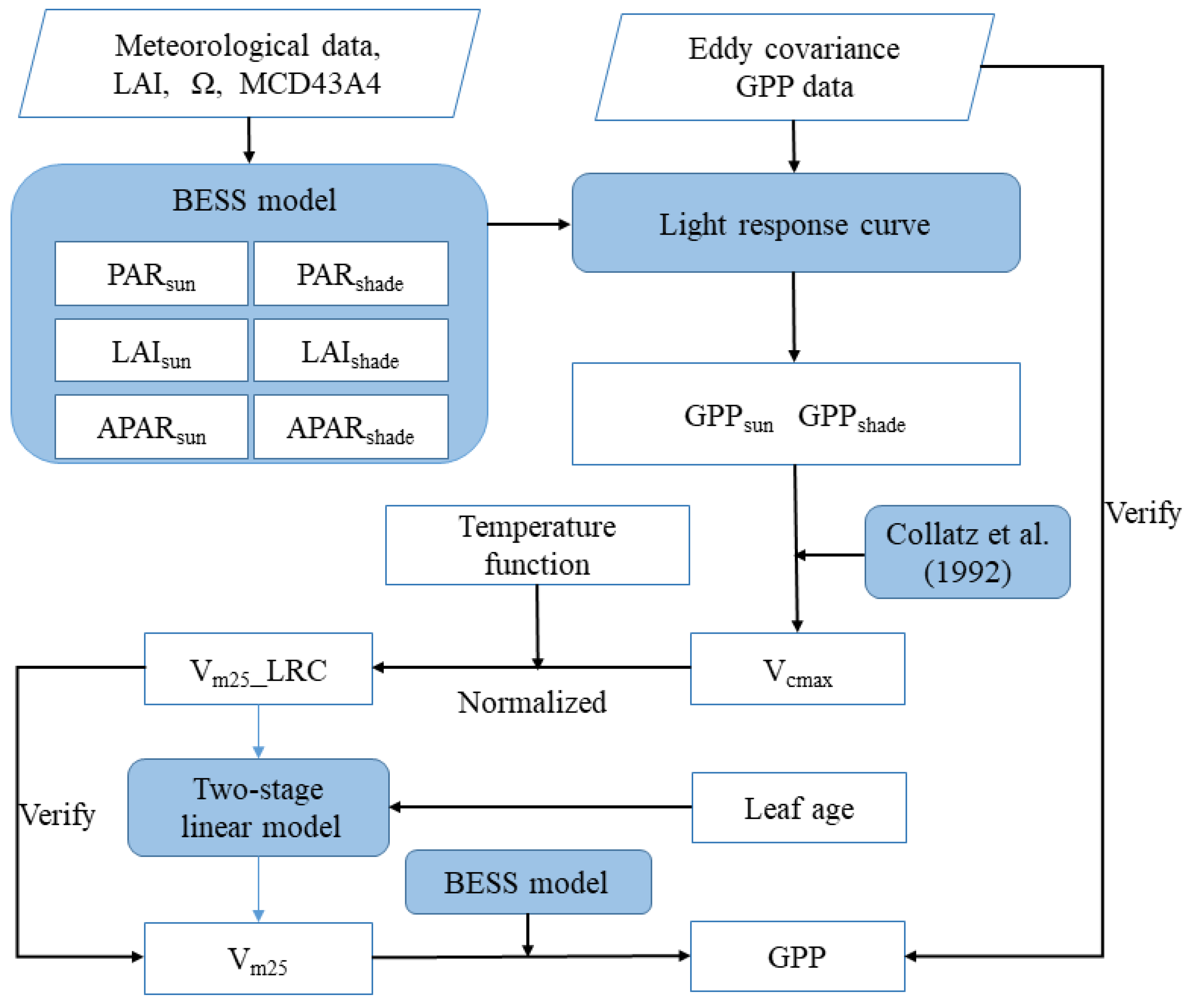
3.1. Inversely Solving Vm25 by Coupling the BESS and LRC

Zheng and Xie inverted the time series of Vm25 by coupling Boreal Ecosystem Productivity Simulator (BEPS) with light response curve (LRC), utilizing EC observations data and remote sensing data from flux sites [31,32]. This method effectively optimizes Vm25 by separating the contributions of sunlit leaves and shade leaves. However, the BEPS model does not account for the physiological process for C4 plants, such as maize [33]. What is more, BEPS employs a fixed Vm25 value. The Breathing Earth System Simulator (BESS) model not only differentiates between sunlit and shaded leaves [56], but also distinguishes between C3 and C4 plants. Additionally, BESS incorporates LAI to account for seasonal variation in Vm25. Therefore, we substituted the BEPS model with the BESS model.

3.1.1. The Separation of Sunlit and Shaded GPP by BESS

In the BESS model, the photosynthesis rate at leaf-level is calculated by Farquhar’s and Collatz’s model [11,12], while a “two-leaf” canopy model is employed to upscale the leaf-level photosynthesis rate to canopy GPP. The total GPP of the canopy is determined by summing the contributions from sunlit leaves and shaded leaves as follows:
G P P = G P P s u n + G P P s h a d e
where GPPsun and GPPshade are the GPP of sunlit and shaded leaves, respectively. GPP can be calculated from photosynthesis rate and the corresponding LAI; therefore, Equation (1) can be expressed as:
GPP = A s u n L A I s u n + A s h a d e L A I s h a d e
where Asun and Ashade are the photosynthesis rates per units of sunlit and shaded leaves, respectively; LAIsun and LAIshade are the LAI of sunlit and shaded leaves, which can be calculated by:
L A I s u n = 2 cos θ 1 e x p 0.5 Ω L A I cos θ
L A I s h a d e = L A I L A I s u n
where θ is solar zenith angle, Ω is the clumping index, and LAI is the leaf area index of the whole canopy.

3.1.2. Photosynthesis Rates of Sunlit and Shaded Leaves Estimated by LRC

Light response curve is a commonly utilized tool to depict the correlation between the photosynthetic rate and photosynthetically active radiation (PAR). The rectangular hyperbola is employed to characterize the shape of the light response curve [78]:
A = α I P α I + P
where A is the gross photosynthesis rate; α is the maximum light use efficiency (LUE) obtained by the initial slope of the curve; I is the absorbed photosynthetically active radiation (APAR) of the leaf per unit; P is the gross photosynthetic rate under saturated radiation.
The light response curves are employed to estimate Asun and Ashade, respectively [31,33]. Then, the total canopy GPP of Equation (2) can be expressed as:
G P P = L A I s u n α I s u n P s u n α I s u n + P s u n + L A I s h a d e α I s h a d e P s h a d e α I s h a d e + P s h a d e
where Isun and Ishade are PAR absorbed by sunlit leaves and shade leaves (APARSun and APARSh), respectively, and are calculated using the two-leaf canopy radiative transfer model in BESS (Appendix B); and Psun and Pshade are given by:
P s u n = P 0 k 1 e k L A I k n L A I k + k n × 1 e k L A I
P s h a d e = P 0 2 c o s θ k n k k n + k e k L A I e k L A I k k L A I 2 c o s θ k n 1 k k n k n 2 + k n k L A I 2 c o s θ 1 e k L A I
where P0 is P on the top of the canopy; kn describes the rate at which leaf nitrogen content decreases with increasing depth into the canopy, and is taken as 0.3 following the previous study [21].
k = 0.5 Ω c o s θ
Here, α and Po represent the two unknown parameters, both of which are contingent on the biological conditions of the leaves. During periods of low incoming radiation, such as in the morning or afternoon, the photosynthetic rate is presumed to be primarily influenced by radiation, leading to the maximum LUE at these times. To determine α for the day, GPP data are selected with incoming PAR less than 350 μmol m−2s−1 for regression analysis against APAR. The resulting slope of this regression is considered as α for the given day. The daily value of P0 is then obtained through the optimization of eddy covariance GPP data after determining α.

3.1.3. The Inversion of Vcmax from Sunlit GPP

According to Collatz’s model:
A = m i n A j , A c R d
where A is the gross photosynthesis; Aj represents the rate of photosynthesis limited by radiation and Ac represents the rate of photosynthesis restricted by Rubisco; Rd is the rate of dark respiration.
When estimating Vcmax through the reversal of Collatz’s method, it is essential that the photosynthetic rate is limited by Vcmax, rather than radiation. In shaded leaves, the photosynthetic rate is primarily regulated by radiation. Conversely, sunlit leaves receive more radiation than shaded leaves; thus, their photosynthetic rate is not controlled by radiation but by Vcmax when incident radiation levels are high. The separation of sunlit and shaded leaves enables the inversion of Vcmax from the GPP of sunlit leaves. For sunlit leaves, when incident radiation levels are low, such as in the early morning, the photosynthetic rate is dependent on radiation. However, as incident radiation increases, it gradually becomes limited by Rubisco. A threshold of 900 μmol m−2s−1 is utilized for radiation levels. When APAR exceeds this threshold, the photosynthetic rate is predominantly limited by Vcmax. Consequently, Vcmax is derived from the GPP of sunlit leaves under such conditions [31].
Once the GPP of sunlit leaves has been separated, the photosynthesis rate of sunlit leaves can be calculated as:
A c = G P P s u n L A I s u n
For C4 plants, according to Collatz’s model [12], when the CO2 fixation is controlled only by Rubisco, Vcmax is calculated as:
V c m a x = A c

3.1.4. Normalizing Vcmax to 25 °C

The inverted Vcmax can be normalized to 25 °C (Vm25) using the temperature function [79]:
V m 25 = V c m a x f T
f T = 1 + e x p 220,000 + 710 T + 273 R T + 273 1
where T is the leaf temperature; and R is the gas constant.

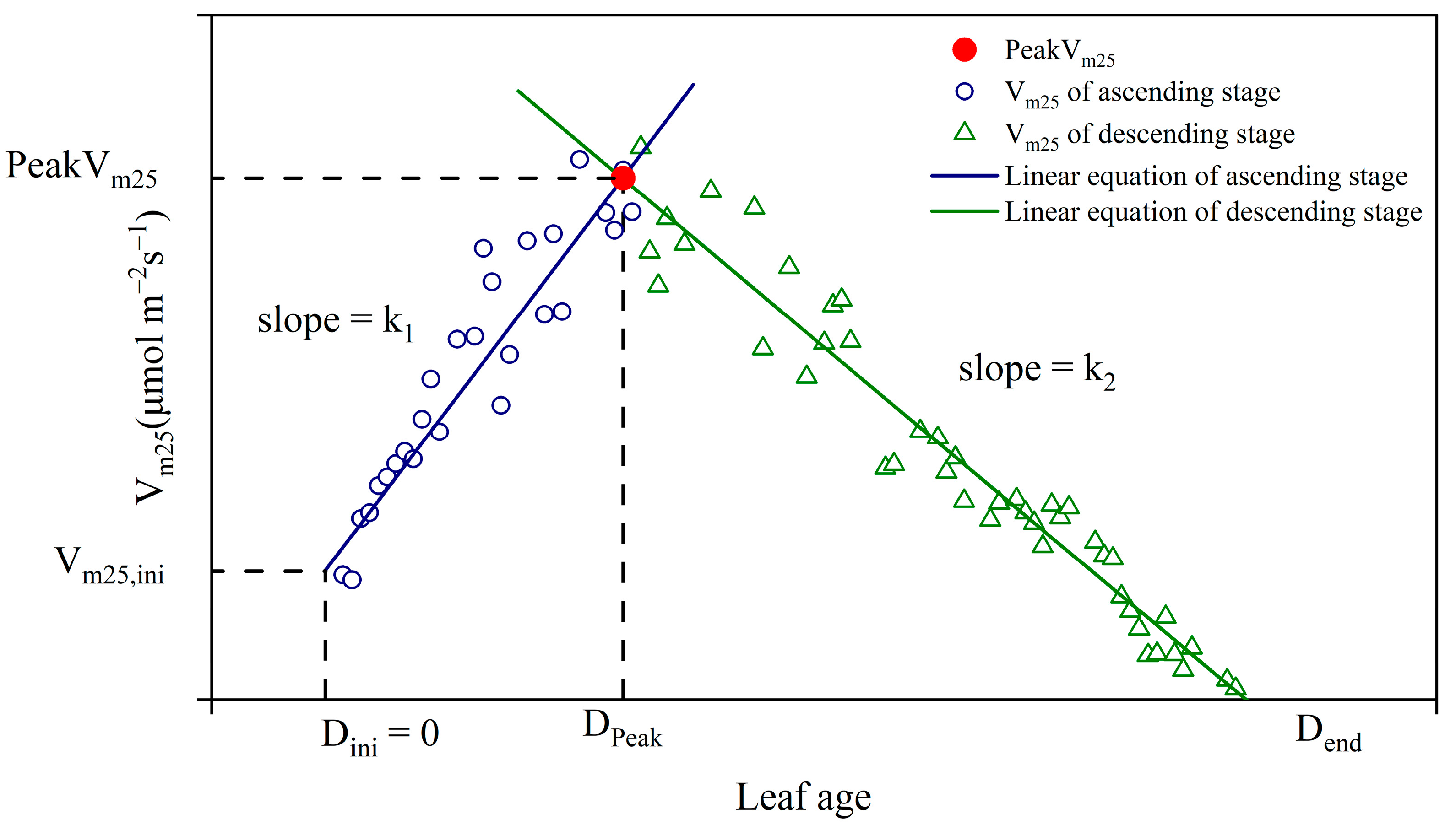
3.2. Two-Stage Linear Model

Crops typically experience rapid growth in the early stages, reaching a peak before gradually aging. Thus, we divided the crop growth period into an ascending phase and a descending phase (Figure 2). According to FAO56 guidelines [80], the rapid growth period of maize typically spans from 35 to 50 days, counting from the date of emergence. Therefore, within this date range, we identified the day with the smallest change in LAI as the cut-off point between the ascending phase and descending phase, denoted as DPeak. We discovered that Vm25 exhibits a stronger correlation with leaf age than with LAI, particularly during the descending phase (Figure 2).
Building upon this discovery, we proposed a Two-stage linear model that utilizes leaf age to simulate Vm25 (Figure 3). In this model, Vm25 is linearly fitted separately for the ascending and descending phases (Equations (16) and (17)). Our Two-stage linear model is as follow:
V m 25 = k 1 × D + V m 25 , i n i         ,             D i n i < D < D P e a k k 2 × D D P e a k         ,           D p e a k D < D e n d
where Dini represents the leaf age when the crop initiates rapid growth, recorded as 0; DPeak represents the leaf age when the Vm25 reaches maximum; Dend denotes the ending leaf age of the crop growth period, typically when the GPP value observed by the flux sites approaches 0; and D represents the current leaf age. k1 and k2 denote the slopes of the ascending and descending stages of crop development, respectively.
k 1 = P e a k V m 25 V m , i n i D P e a k
k 2 = P e a k V m 25 D e n d D P e a k
Leaf age is commonly used to describe the growth status and developmental stage of plants. Its specific definition and calculation methods can vary depending on the research objectives and plant species. In our study, leaf age refers to the physical age of the plant, meaning the actual time from emergence to the current leaf development stage, measured in days. The emergence dates for US-Ne1, US- Ne2, and US-Ne3 can be obtained from the literature. For the Daman and Fenzidi, the emergence dates can be inferred from the changing trends in LAI values.

3.3. Model Validation

3.3.1. Calibration and Validation of Vm25

Data from one-third of the years were utilized for calibrating the PeakVm25 (Section 3.2), while data from the remaining two-thirds of years were employed to validate the accuracy of the Two-stage linear model. It is worth mentioning that the estimation of Vm25 for leaves operating under low radiation conditions is typically less accurate. The cumulative effect of errors in various underlying assumptions can lead to a relatively low signal-to-noise ratio [81]. Thus, Vm25 values corresponding to low radiation were excluded.
The PeakVm25 was calculated for the three US sites (US-Ne1, US-Ne2, US-Ne3) and the two Chinese sites (Daman, Fenzidi) separately, to account for the difference in maize species. To determine the value of the PeakVm25, data from the first third of each year at each site were selected. Linear regression between Vm25 inverted by LRC and leaf age was performed for both the ascending phase and descending phase, respectively. The average PeakVm25 value for the first third years of the three US sites and the two Chinese sites are 65 and 38 μmol m−2s−1 (rounded to an integer), respectively. Note that Vm25,ini is difficult to estimate when the GPP is close to zero or negative at the beginning of the growth period. Thus, the Vm25 at the beginning of the growth period is set as 10 μmol m−2s−1, the median of the LRC inverted Vm25 during this period (5–15 μmol m−2s−1).

3.3.2. Comparison with the Vm25 Obtained by BESS

In the BESS model, seasonal variation in Vm25 is taken into account [56,82]. It is assumed that the seasonal pattern of Vm25 followed the seasonal pattern of LAI [83]. Vm25 experiences a rapid increase during leaf development, reaching its peak in early leaf maturity, followed by a decline during senescence, irrespective of species. The date corresponding to the peak LAI value is identified, and the Vm25 for that date was quantified (PeakVm25). Subsequently, Vm25 over the season is calculated as:
V m 25 = V m 25 , m i n + L A I L A I m a x × P e a k V m 25 V m 25 , m i n
where LAImax and LAI represent the maximum and current leaf area index, respectively, throughout the growing period. In the original BESS model, the PeakVm25 value of C4 crops was uniformly set as 33 μmol m−2s−1, without distinction among crop types. Vm25,min = 0.3 × PeakVm25.
In the original BESS model (Equation (18)), the PeakVm25 value of C4 crops was uniformly set at 33 μmol m−2s−1, without differentiation among crop species. In our model, the calibrated PeakVm25 value was substituted into the original BESS model to calculate Vm25 (hereafter referred to as “BESS_P”), and then the performances of the original BESS, BESS_P and our Two-stage linear model in simulating Vm25 were compared against the Vm25 inversely solved by coupling the BESS and LRC using EC data.

3.3.3. Comparison with the GPP Obtained by BESS

Then, the original BESS model, BESS_P model, and the BESS model coupled with the Two-stage linear model (hereinafter referred to as “BESS_TL”) were used to calculate GPP. These simulated GPP values were then compared with the GPP values measured at the flux sites to evaluate the performance of each model. This comparison helps in assessing the accuracy and reliability of each method in simulating GPP.

4. Results

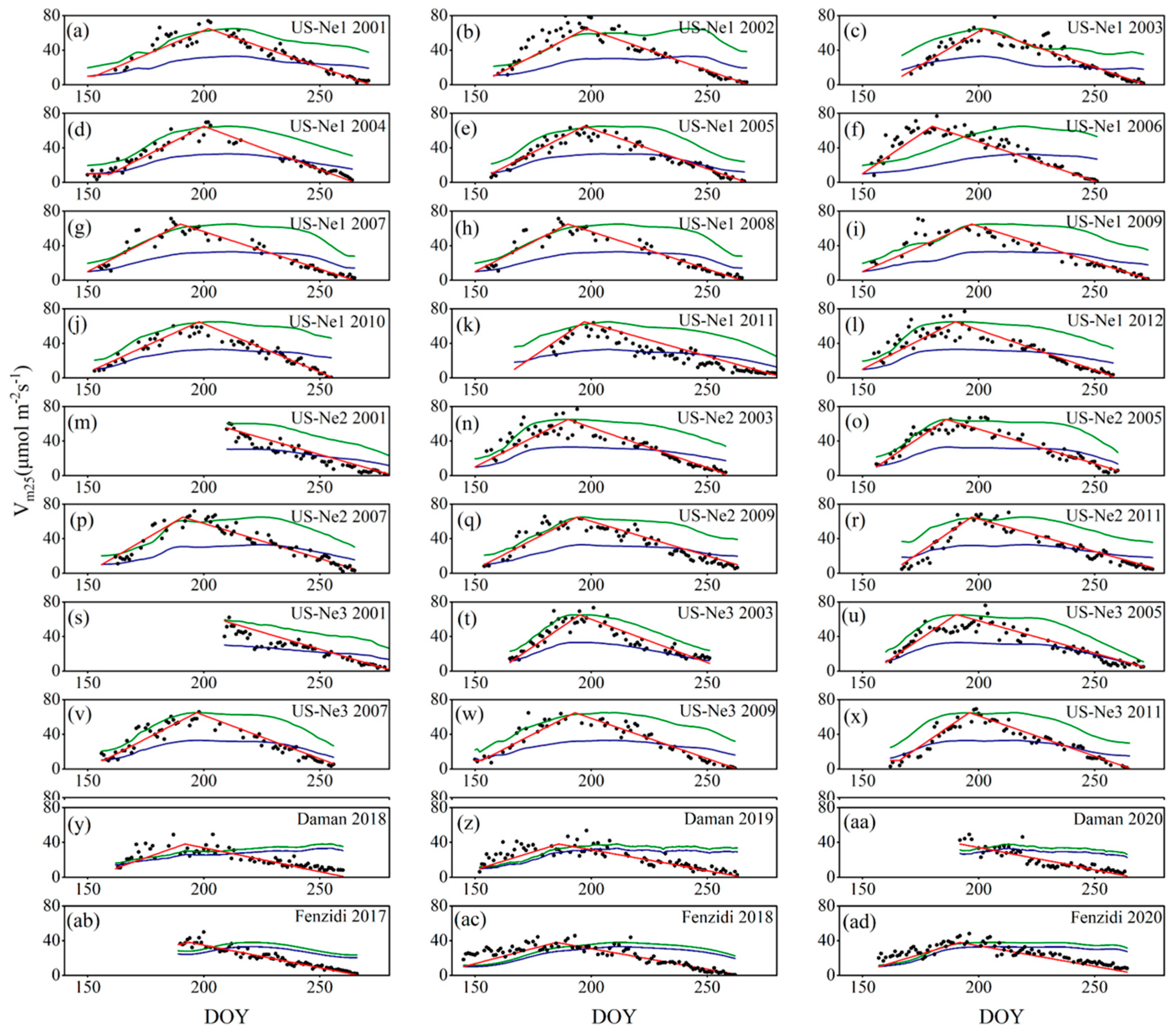
4.1. Calibration and Validation of Vm25

To assess the performance of the Two-stage linear model (Equation (15)), the simulated Vm25 was compared with the Vm25 inversely solved by coupling the BESS and LRC using EC data (Figure 4, Table 2). Notably, the simulated Vm25 aligns closely with that from LRC for both the calibration and validation samples at each site (Figure 4, Table 2). The performance of the Two-stage linear model was exceptional for the US-Ne2 and US-Ne3 sites, yielding R2 values of 0.88 and 0.87, RMSE values of 6.82 μmol m−2s−1 for both, whereas the performance was not as good for Daman (R2 = 0.71; RMSE = 6.44 μmol m−2s−1), due to the pronounced fluctuation in Vm25 during the early stages of the growth period at Daman (Figure 5y, z).

4.2. Comparison with the Vm25 Obtained by BESS

The Vm25 calculated by BESS, BESS_P and our Two-stage linear model were compared in simulating the time series of Vm25 inversely solved by coupling the BESS and LRC using EC data at the five flux sites (Figure 5). Unfortunately, the flux data for Daman in 2020 and Fenzidi in 2017 are incomplete; and due to the partial lack of remote sensing and meteorological data, the Vm25 inverted by LRC for US-Ne1 and US-Ne2 sites in 2001 is also incomplete. The BESS model consistently underestimates Vm25 throughout the growth period due to the fixed low PeakVm25 value, with the discrepancy becoming particularly noticeable during the middle stages of the growth period. Conversely, towards the end of the growth period when Vm25 values are low, BESS tends to overestimate Vm25. BESS_P, which employs the same modeling approach as BESS but adjusts the PeakVm25 parameter, exhibiting a somewhat improved performance in estimating the trend of Vm25 during the early growth phase. However, during the declining stage of Vm25, BESS_P tends to significantly overestimate the values. Due to the same formula structure, the R2 between the calculated Vm25 of both methods and the verified values remains consistent, ranging from 0.01 to 0.67 (Table 2). The RMSE of the BESS model ranges from 13.25 to 18.93 μmol m−2s−1 and the RMSE of the BESS_P ranges from 15.30 to 25.07 μmol m−2s−1. Despite the adjustment in PeakVm25, both BESS and BESS_P demonstrate poor performance in fitting the trend in Vm25 across all sites. The observations reveal a distinct pattern of Vm25 initially rising before declining, and our Two-stage linear model effectively captures this seasonal variation in Vm25, with R2 ranges from 0.71 to 0.88 and RMSE ranges from 5.40 to 7.54 μmol m−2s−1. During the early stages of crop growth, Vm25 generally exhibits an upward trajectory, albeit with significant diurnal fluctuations. Conversely, in the descending phase, Vm25 tends to display a more linear decline with reduced fluctuation.

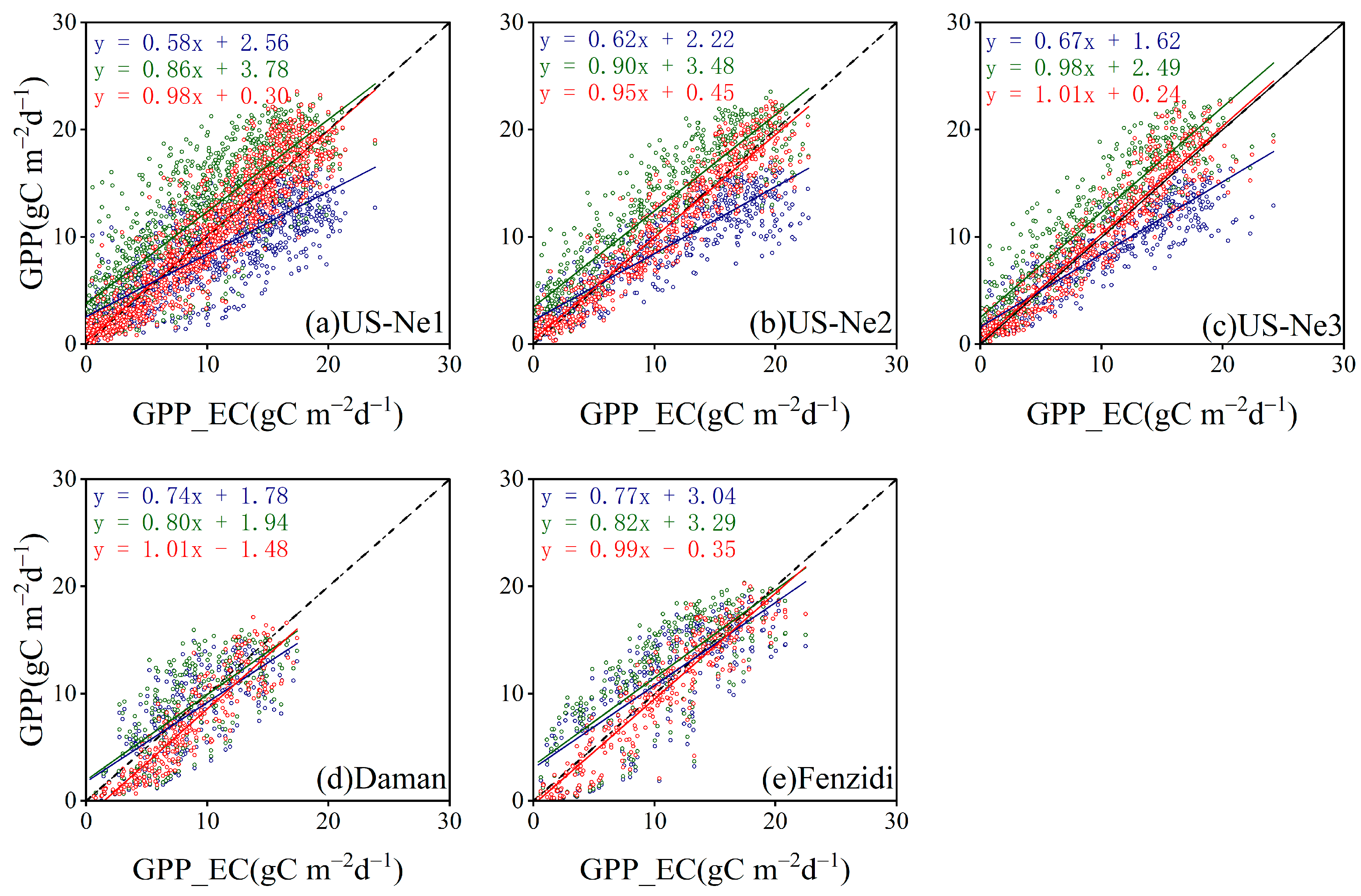
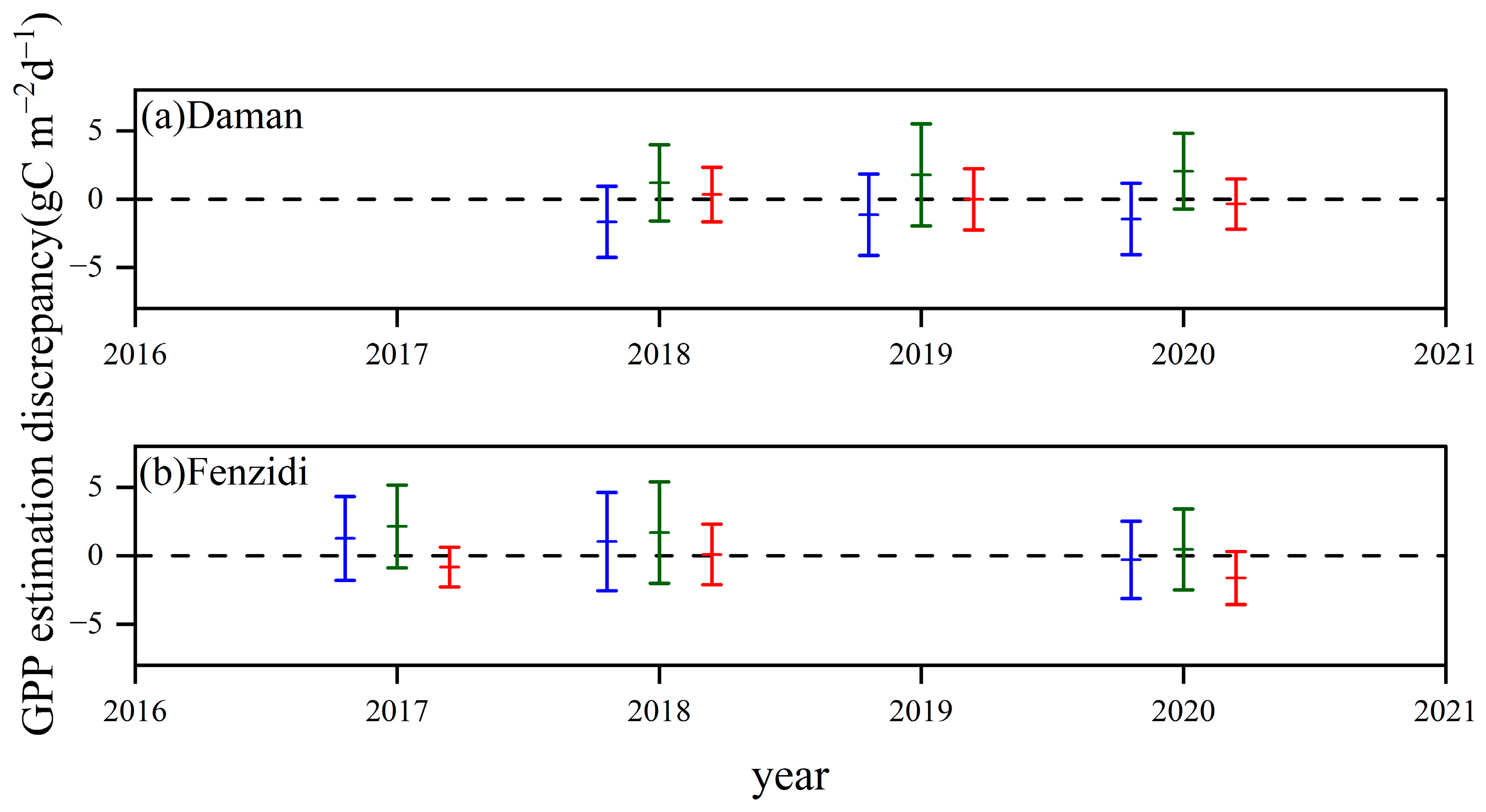
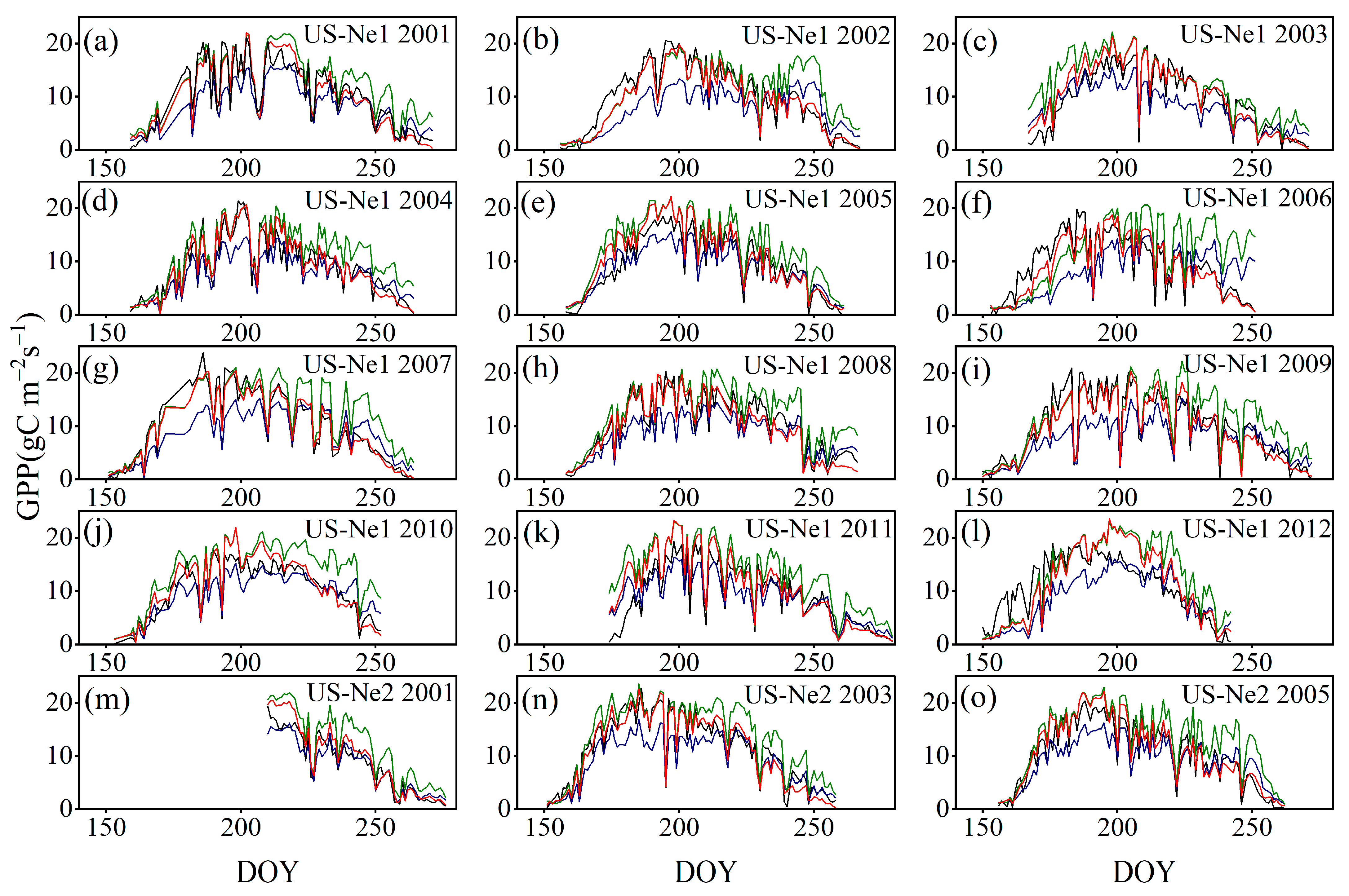
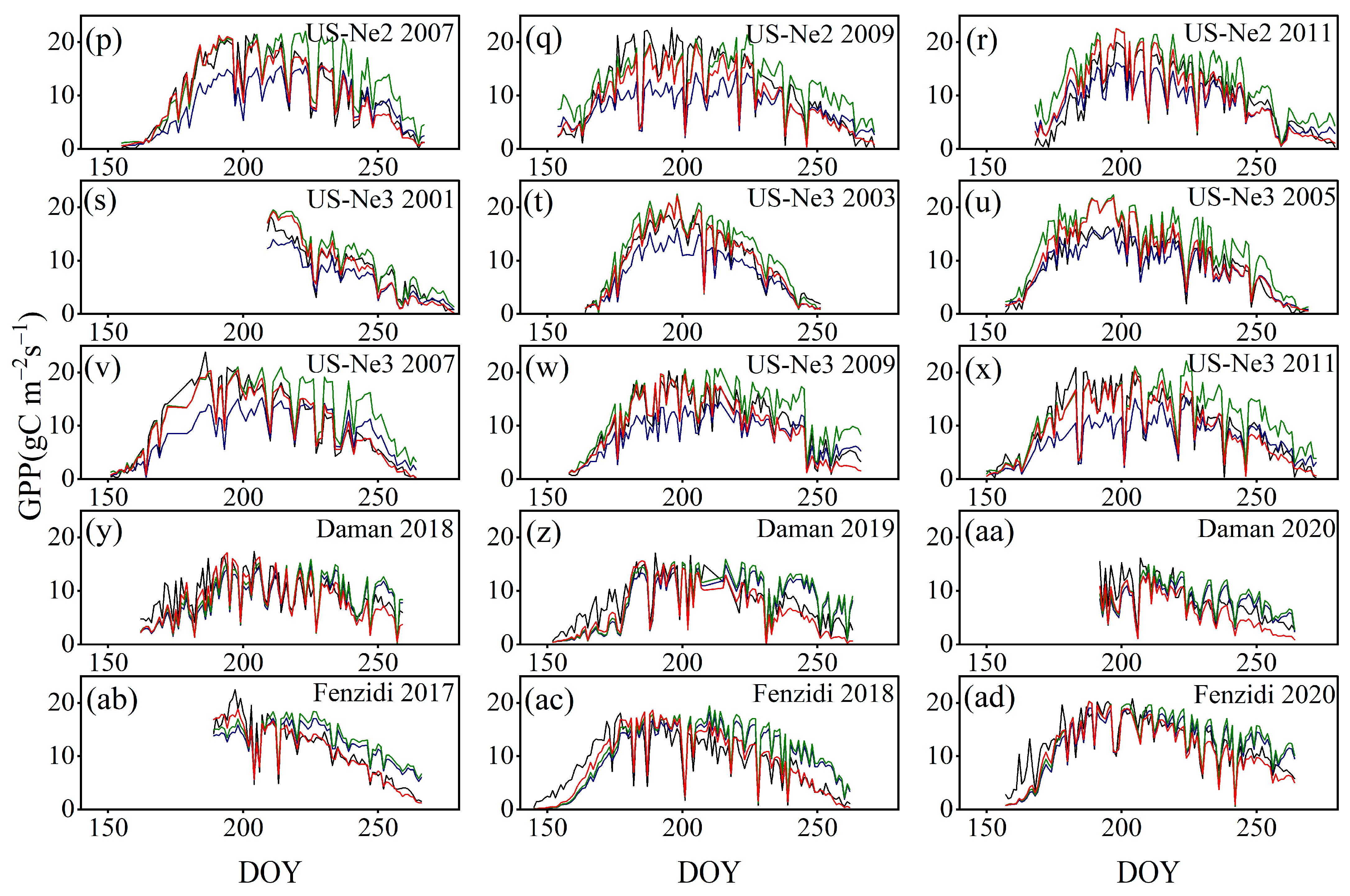
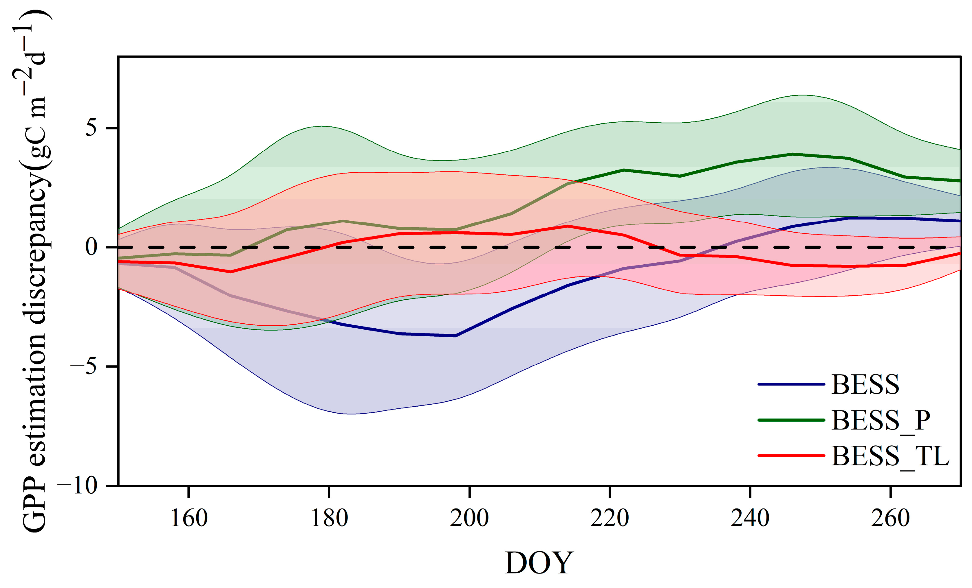
4.3. Comparison with the GPP Obtained by BESS

To evaluate the role of the Two-stage linear model in improving GPP simulation, we compared the GPP simulation results using BESS, BESS_P and our Two-stage linear model for calculating Vm25, and validated them with flux site GPP data (Figure 6, Table 3). The results indicate that the original BESS model consistently underestimates GPP across all five sites. On average, GPP is underestimated by 12.60%, with the most significant underestimation observed at US-Ne2 (16.29%). Similarly, BESS_P generally overestimates GPP, averaging 20.73% across all sites, with the most significant overestimation recorded at US-Ne1 (24.05%). In contrast, the GPP simulated by BESS incorporating our Two-stage linear model exhibits a strong correlation with the flux site’s observed GPP data, with RMSE ranging from 2.03 to 2.32 gC m−2d−1 and R2 ranging from 0.82 to 0.90. On average, GPP is only underestimated by 0.85% across all sites. The most substantial underestimation occurs at Daman (16.38%), while the most significant overestimation is at Fenzidi (4.60%). The simulation result of BESS_TL significantly outperform the BESS and BESS_P in GPP estimation.
To better reveal the role of the Two-stage linear model in improving GPP simulation, the discrepancy of the annual GPP estimation by BESS, BESS_P and BESS_TL were compared (Figure 7 and Figure 8). The mean GPP estimation discrepancy by BESS, BESS_P and BESS_TL are −1.56, 2.39 and 0.12 gC m−2d−1 in US-Ne1, respectively, with the corresponding standard deviations of 3.35, 3.30 and 2.29 gC m−2d−1 (Table 4). Except for the Daman site, the means and standard deviations of GPP discrepancy of BESS_TL estimation are closer to 0 for most years compared to the BESS and BESS_P estimation (Table 4). At the Daman site, although the absolute value of the mean GPP estimation discrepancy of BESS_TL is greater than that of BESS, the standard deviation of BESS_TL GPP estimation discrepancy remains the smallest. Thus, it can be concluded that BESS_TL effectively enhances the simulation accuracy of GPP.
To provide a clearer view of the simulation results of the three methods, the seasonal variation in the GPP difference between the simulated GPP and EC observations is represented in Figure 9 and Figure 10. Figure 9 displays the annual simulation results for each site, while Figure 10 presents the multi-year average simulation outcomes across all sites. Significant seasonal differences are evident in the simulation outputs of all three methods. The original BESS model tends to slightly overestimate GPP towards the end of the growth period and underestimates during other times, particularly in the mid-growth period, where the underestimation is pronounced. Conversely, BESS_P demonstrates satisfactory simulations only during the early growth period, followed by a gradual overestimation of GPP. BESS_TL outperforms the other two methods in capturing seasonal shifts in GPP. The discrepancy between the simulated GPP and EC values remains relatively close to zero. GPP is slightly underestimated during the early and late growth stages and slightly overestimated during the mid-growth stage. Overall, BESS_TL demonstrates a more balanced performance across different growth stages compared to BESS and BESS_P.

5. Discussion

5.1. Foundation of Vm25 Estimation

This study highlights the importance of considering seasonal changes in the photosynthetic capacity of crops. However, estimating the temporal changes in Vm25 remains challenging. The method to inverting the time series of Vm25 by coupling the BEPS model and LRC has already been proposed. However, the BEPS model does not account for C4 plants [31,32]. In our research, we addressed this challenge by inverting Vm25 for five maize sites through the coupling of the BESS model with LRC. This approach enabled us to estimate Vm25 without relying on extensive gas exchange experiments. To achieve this, we utilized field measurements of EC data and remote sensing data. The BESS model, which replaces the original BEPS model, incorporates specific considerations for the photosynthesis of C4 plants like maize [56]. After removing the data from periods of low radiation, Vm25 exhibited a significant trend of initially increasing and then decreasing (Figure 5). Furthermore, Vm25 showed a strong correlation with leaf age when the growing period was divided into two phases (Figure 2). This relationship provides the basis for our research.

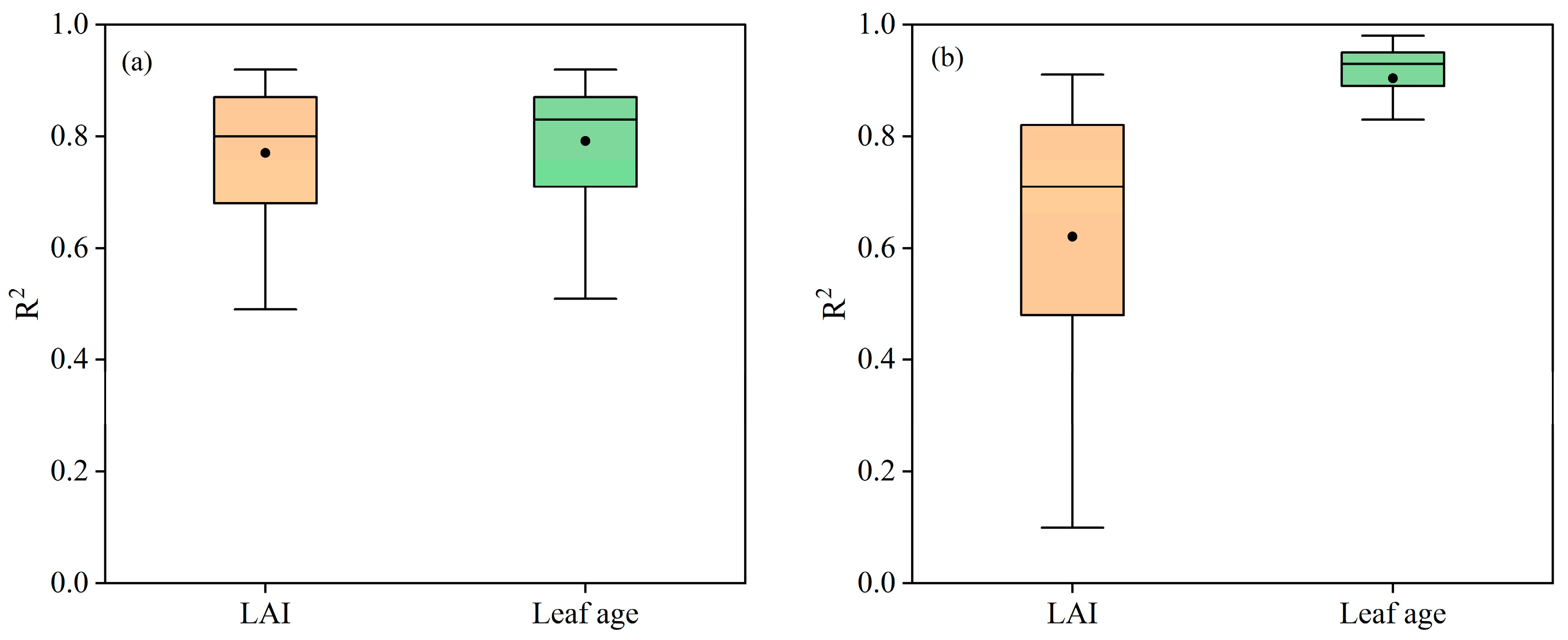
5.2. The Advantages of Leaf Age as a Vm25 Predictor

Annual plants complete their entire life cycle within one growing season. Starting from seeds, they progress through stages of germination, growth, flowering, fruiting, and ultimately die, all within a single year. In contrast, perennials continue to grow and reproduce for several years or more. Compared to perennial plants, using annual plants as research subjects eliminates the need to consider interannual influences and allows for easier identification of their developmental stages. This simplification makes it more straightforward to study the relationship between leaf age and Vm25.
Our Two-stage linear model takes the advantage of leaf age and effectively captures the Vm25 seasonal variation with the crop growth processes. Maize, being annual plants, undergo significant changes in photosynthetic capacity throughout their growth cycle due to various physiological characteristics. Typically, Vm25 exhibits only one peak value during the entire crop growth period [33]. This uniqueness of the crop is the basis for our proposed model. In our model, the basic assumption is that the photosynthetic capacity increases during leaf development, reaching a maximum in spring or early summer, stabilizing or gradually decreasing in summer, and further decreasing during senescence [6,84]. Comparably, our model, in which Vm25 is quantified with leaf age, can perform well due to the strong correlation between Vm25 and leaf age (Figure 2). Now, it is understandable that the performance of the existing empirical relationships established between Vm25 and other variables, such as NLeaf, Chll, and photoperiod, is basically determined by the similarity of that variable to the leaf age [7,8,40,85]. Also, the photosynthetic capacity and environmental factors are often mismatched [57].
For the estimation of Vm25, our Two-stage linear model outperforms both the original BESS model and BESS_P. The main difference between the original BESS model and BESS_P is the PeakVm25: PeakVm25 in the original BESS model is fixed, whereas the PeakVm25 in the BESS_P is the same as the PeakVm25 in our Two-stage linear model. Thus, solely improving the PeakVm25 cannot solve the problem. In the original BESS model and BESS_P, LAI is used to seasonalize Vm25 [56]. However, it is proven that the correlation between Vm25 and LAI is not as strong as leaf age in the later half stage of crop growth (Figure 2) because the leaves turn yellow and senesce with the senescence of crops, but the change in LAI is not significant. Furthermore, the BESS model coupled with the Two-stage linear model (BESS_TL) has significantly improved the simulation of GPP. Across the five maize sites, BESS_TL only underestimated GPP by an average of 0.85%. In contrast, the original BESS model underestimated GPP by an average of 12.60%, and the BESS_P model overestimated GPP by an average of 20.73%. The superior performance of our Two-stage linear model underscores the importance of considering PeakVm25 and leaf age in accurately modeling Vm25.

5.3. Readily Available Leaf Age

Leaf age, an important indicator of crop physiological characteristics, is usually relatively easy to obtain. The emergence date can be directly observed in the field, allowing for straightforward counting to determine leaf age [62]. Additionally, remote sensing technologies offer a powerful tool for estimating leaf age across large areas of farmland [86,87]. By calculating vegetation indices from remote sensing images, we can indirectly assess the growth stage of leaves. These indices exhibit specific patterns of change as the leaves progress from young to mature and eventually to senescent stages. By analyzing these patterns, we can accurately infer leaf age.

5.4. Model Limitations

Due to data availability, our Two-stage linear model was only validated with maize data from five flux sites. Its applicability to other sites relies on the quality of their own flux data. Also, our Two-stage linear model is derived from maize sites, and its applicability to other vegetation types requires further validation. While other vegetation types have also demonstrated a close correlation between Vm25 and leaf age [8,58,63,64], extending this method to other vegetation types, such as perennial plants, presents additional challenges. Perennials often have canopies that consist of leaves at various stages of development, ranging from young and fully functional to older and senescent leaves [63]. This variation necessitates a more nuanced approach to modeling Vm25 in perennials, one that can account for the complex age structure of their canopies [58].

6. Conclusions

As numerous studies have highlighted, Vm25 is a crucial parameter for calculating the photosynthesis rate. The accurate estimation of Vm25 is essential for the regional and global modeling of ecological systems. Although various indicators have been developed to characterize Vm25, accurately quantifying its dynamic changes remains challenging.
(1) 
Vm25 inversion: Considering the special photosynthetic process of C4 plants, we replaced the BEPS model with the BESS model coupled with the LRC to invert Vm25 at five maize sites. This method allowed us to obtain continuous Vm25 values throughout the growth period, enabling a detailed study of Vm25 variation trends.
(2) 
Two-Stage Linear Model Development: We developed a new Two-stage linear model to determine the dynamics changes in maize Vm25. This method divides Vm25 into two stages during the growth process and uses leaf age as the key variable in the simulation, effectively capturing the seasonal variation characteristics of Vm25. Additionally, compared to using a fixed value, this method allows for the calibration of the PeakVm25 value, thereby enhancing model accuracy.
(3) 
Model Performance and Comparison: The Two-stage linear method more accurately simulated the variation trend of Vm25 compared to the Vm25 of the original BESS model. Furthermore, implementing this method significantly improved the simulation results of GPP. BESS_TL outperforms the other two methods in this study, showing higher R2 and lower RMSE at each site. The GPP simulated by BESS_TL at both interannual and seasonal levels deviated less from the EC GPP. Overall, the developed Vm25 estimation method enhances the accuracy of farmland GPP simulation.

Author Contributions

Conceptualization, X.Z. and Z.H.; methodology, X.Z. and S.W.; validation, X.Z. and S.W.; data curation, W.W. and Y.R.; writing—original draft preparation, X.Z.; writing—review and editing, C.W. and Z.H.; supervision, C.Z.; project administration, C.Z. and Z.H.; funding acquisition, Z.H. All authors have read and agreed to the published version of the manuscript.

Funding

This research was funded by the National Natural Science Foundation of China (Grant Numbers: 52130902 and 52279050), and the National Key Research and Development Program of China (Grant Number: 2021YFD1900603). Research project of Inner Mongolia (NMKJXM202208).

Data Availability Statement

The original contributions presented in the study are included in the article further inquiries can be directed to the corresponding author.

Acknowledgments

We are grateful to the data providers at US-Ne1, US-Ne2, US-Ne3, and Daman sites. The dataset of Daman is provided by National Tibetan Plateau Data Center (http://data.tpdc.ac.cn (accessed on 1 March 2023)). The dataset of US-Ne1, US-Ne2 and US-Ne3 is provided by FLUXNET2015 (FLUXNET). The authors would like to thank the Editor and all reviewers whose insightful suggestions have significantly improved this paper.

Conflicts of Interest

The authors declare no conflicts of interest.

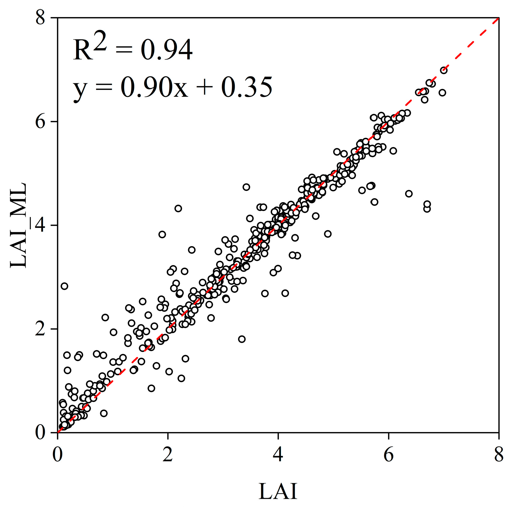
Appendix A. Result of Machine Learning Simulation of LAI

Figure A1. Machine learning training result for LAI using ExtraTreesRegressor.
Remotesensing 16 02747 g0a1

Appendix B. Two-Leaf Canopy Radiative Transfer Model in BESS

A two-leaf canopy radiative transfer model is used to calculate PAR absorbed by sunlit leaves and shade leaves [56]. This method modified the PAR penetration model [88] by incorporating foliar clumping and reflected PAR from the soil.
The total absorbed incoming PAR by the canopy is
Q P = 1 ρ c b P I P b 0 1 e x p k P b L c Ω + 1 ρ c d P I P d 0 1 e x p k P d L c Ω
where I P b 0 and I P d 0 are direct beam and diffuse PAR at the top of the canopy, respectively. L c indicates the leaf area index. ρ c b P and ρ c d P are canopy reflectance for beam and diffuse PAR, respectively. k P b and k P d are the extinction coefficient for beam and scattered beam PAR, and for diffuse and scattered diffuse PAR, respectively.
The absorbed incoming beam PAR by sunlit leaves is
Q P b S u n = I P b 0 1 σ P A R 1 e x p k b L c Ω
where σ P A R is the leaf scattering coefficient for PAR. k b is the extinction coefficient for black leaves.
The absorbed incoming diffuse PAR by sunlit leaves is
Q P d S u n = I P d 0 1 ρ c d P 1 e x p k P d + k b L c Ω k P d k P d + k b
The absorbed incoming scattered PAR by sunlit leaves is
Q P s S u n = I P b 0 1 ρ c b P 1 e x p k P b + k b L c Ω k P b k P b + k b 1 σ P A R 1 e x p 2 k b L c Ω 2
The total absorbed incoming PAR by sunlit leaves is
Q P S u n = Q P b S u n + Q P d S u n + Q P s S u n
The total absorbed incoming PAR by shade leaves is
Q P S h = Q P Q P S u n
A portion of the incoming PAR passes through the canopy to the soil surface and is reflected upward into the canopy, which may be important in an open canopy with bright background. The PAR absorbed by sunlit leaves due to soil reflection is
Q P S u n = 1 ρ c b P I P b 0 + 1 ρ c d P I P d 0 Q P S u n + Q P S h × ρ s P × exp k P d L c Ω
where ρ s P is the soil reflectance for PAR.
The PAR absorbed by shade leaves due to soil reflection is
Q P S h = 1 ρ c b P I P b 0 + 1 ρ c d P I P d 0 Q P S u n + Q P S h × ρ s P × 1 e x p k P d L c Ω
The total PAR absorbed by sunlit and shade leaves is
A P A R S u n = Q P S u n + Q P S u n
A P A R S h = Q P S h + Q P S h

References

  1. Beer, C.; Reichstein, M.; Tomelleri, E.; Ciais, P.; Jung, M.; Carvalhais, N.; Rodenbeck, C.; Arain, M.A.; Baldocchi, D.; Bonan, G.B.; et al. Terrestrial gross carbon dioxide uptake: Global distribution and covariation with climate. Science 2010, 329, 834–838. [Google Scholar] [CrossRef] [PubMed]
  2. Li, X.L.; Liang, S.L.; Yu, G.R.; Yuan, W.P.; Cheng, X.; Xia, J.Z.; Zhao, T.B.; Feng, J.M.; Ma, Z.G.; Ma, M.G.; et al. Estimation of gross primary production over the terrestrial ecosystems in China. Ecol. Model. 2013, 261, 80–92. [Google Scholar] [CrossRef]
  3. Yuan, W.P.; Liu, S.G.; Yu, G.R.; Bonnefond, J.M.; Chen, J.Q.; Davis, K.; Desai, A.R.; Goldstein, A.H.; Gianelle, D.; Rossi, F.; et al. Global estimates of evapotranspiration and gross primary production based on MODIS and global meteorology data. Remote Sens. Environ. 2010, 114, 1416–1431. [Google Scholar] [CrossRef]
  4. Smith, N.G.; Keenan, T.F.; Colin Prentice, I.; Wang, H.; Wright, I.J.; Niinemets, Ü.; Crous, K.Y.; Domingues, T.F.; Guerrieri, R.; Ishida, F.Y.; et al. Global photosynthetic capacity is optimized to the environment. Ecol. Lett. 2019, 22, 506–517. [Google Scholar] [CrossRef] [PubMed]
  5. Zhu, X.J.; Yu, G.R.; Wang, Q.F.; Gao, Y.N.; He, H.L.; Zheng, H.; Chen, Z.; Shi, P.L.; Zhao, L.; Li, Y.N.; et al. Approaches of climate factors affecting the spatial variation of annual gross primary productivity among terrestrial ecosystems in China. Ecol. Indic. 2016, 62, 174–181. [Google Scholar] [CrossRef]
  6. Miner, G.L.; Bauerle, W.L. Seasonal responses of photosynthetic parameters in maize and sunflower and their relationship with leaf functional traits. Plant Cell Environ. 2019, 42, 1561–1574. [Google Scholar] [CrossRef]
  7. Rogers, A.; Medlyn, B.E.; Dukes, J.S.; Bonan, G.; von Caemmerer, S.; Dietze, M.C.; Kattge, J.; Leakey, A.D.; Mercado, L.M.; Niinemets, U.; et al. A roadmap for improving the representation of photosynthesis in Earth system models. New Phytol. 2017, 213, 22–42. [Google Scholar] [CrossRef] [PubMed]
  8. Wang, S.Q.; Li, Y.; Ju, W.M.; Chen, B.; Chen, J.H.; Croft, H.; Mickler, R.A.; Yang, F.T. Estimation of Leaf Photosynthetic Capacity From Leaf Chlorophyll Content and Leaf Age in a Subtropical Evergreen Coniferous Plantation. J. Geophys. Res. Biogeosci. 2020, 125, e2019JG005020. [Google Scholar] [CrossRef]
  9. Zhang, Y.Q.; Kong, D.D.; Gan, R.; Chiew, F.H.S.; McVicar, T.R.; Zhang, Q.; Yang, Y.T. Coupled estimation of 500 m and 8-day resolution global evapotranspiration and gross primary production in 2002-2017. Remote Sens. Environ. 2019, 222, 165–182. [Google Scholar] [CrossRef]
  10. Liu, J.; Chen, J.M.; Cihlar, J. Mapping evapotranspiration based on remote sensing: An application to Canada’s landmass. Water Resources Res. 2003, 39, 1189. [Google Scholar] [CrossRef]
  11. Farquhar, G.D.; Caemmerer, S.V.; Berry, J.A. A biochemical model of photosynthetic assimilation in leaves of C3 species. Planta 1980, 149, 67–90. [Google Scholar] [CrossRef]
  12. Collatz, G.J.; Ribas-Carbo, M.; Berry, J.A. Coupled Photosynthesis-Stomatal Conductance Model for Leaves of C4 Plants. Aust. J. Plant Physiol. 1992, 19, 519–538. [Google Scholar] [CrossRef]
  13. Lebauer, D.S.; Wang, D.; Richter, K.T.; Davidson, C.C.; Dietze, M.C. Facilitating feedbacks between field measurements and ecosystem models. Ecol. Monogr. 2013, 83, 133–154. [Google Scholar] [CrossRef]
  14. Bonan, G.B.; Lawrence, P.J.; Oleson, K.W.; Levis, S.; Jung, M.; Reichstein, M.; Lawrence, D.M.; Swenson, S.C. Improving canopy processes in the Community Land Model version 4 (CLM4) using global flux fields empirically inferred from FLUXNET data. J. Geophys. Res. Biogeosci. 2011, 116, G02014. [Google Scholar] [CrossRef]
  15. Medvigy, D.; Jeong, S.J.; Clark, K.L.; Skowronski, N.S.; Schafer, K.V.R. Effects of seasonal variation of photosynthetic capacity on the carbon fluxes of a temperate deciduous forest. J. Geophys. Res. Biogeosci. 2013, 118, 1703–1714. [Google Scholar] [CrossRef]
  16. Grassi, G.; Vicinelli, E.; Ponti, F.; Cantoni, L.; Magnani, F. Seasonal and interannual variability of photosynthetic capacity in relation to leaf nitrogen in a deciduous forest plantation in northern Italy. Tree Physiol. 2005, 25, 349–360. [Google Scholar] [CrossRef] [PubMed]
  17. Yuan, D.K.; Zhang, S.; Li, H.J.; Zhang, J.H.; Yang, S.S.; Bai, Y. Improving the Gross Primary Productivity Estimate by Simulating the Maximum Carboxylation Rate of the Crop Using Machine Learning Algorithms. IEEE Trans. Geosci. Remote Sens. 2022, 60, 4413115. [Google Scholar] [CrossRef]
  18. Qian, X.J.; Liu, L.Y.; Chen, X.D.; Zarco-Tejada, P. Assessment of Satellite Chlorophyll-Based Leaf Maximum Carboxylation Rate (Vcmax) Using Flux Observations at Crop and Grass Sites. IEEE J. Sel. Top. Appl. Earth Obs. Remote Sens. 2021, 14, 5352–5360. [Google Scholar] [CrossRef]
  19. Houborg, R.; Cescatti, A.; Migliavacca, M.; Kustas, W.P. Satellite retrievals of leaf chlorophyll and photosynthetic capacity for improved modeling of GPP. Agric. For. Meteorol. 2013, 177, 10–23. [Google Scholar] [CrossRef]
  20. Zhang, Y.; Guanter, L.; Berry, J.A.; Joiner, J.; van der Tol, C.; Huete, A.; Gitelson, A.; Voigt, M.; Kohler, P. Estimation of vegetation photosynthetic capacity from space-based measurements of chlorophyll fluorescence for terrestrial biosphere models. Glob. Chang. Biol. 2014, 20, 3727–3742. [Google Scholar] [CrossRef]
  21. Chen, J.M.; Mo, G.; Pisek, J.; Liu, J.; Deng, F.; Ishizawa, M.; Chan, D. Effects of foliage clumping on the estimation of global terrestrial gross primary productivity. Glob. Biogeochem. Cycles 2012, 26, GB1019. [Google Scholar] [CrossRef]
  22. Gan, R.; Zhang, Y.Q.; Shi, H.; Yang, Y.T.; Eamus, D.; Cheng, L.; Chiew, F.H.S.; Yu, Q. Use of satellite leaf area index estimating evapotranspiration and gross assimilation for Australian ecosystems. Ecohydrology 2018, 11, e1974. [Google Scholar] [CrossRef]
  23. Dillen, S.Y.; Op de Beeck, M.; Hufkens, K.; Buonanduci, M.; Phillips, N.G. Seasonal patterns of foliar reflectance in relation to photosynthetic capacity and color index in two co-occurring tree species, Quercus rubra and Betula papyrifera. Agric. For. Meteorol. 2012, 160, 60–68. [Google Scholar] [CrossRef]
  24. Croft, H.; Chen, J.M.; Luo, X.; Bartlett, P.; Chen, B.; Staebler, R.M. Leaf chlorophyll content as a proxy for leaf photosynthetic capacity. Glob. Chang. Biol. 2017, 23, 3513–3524. [Google Scholar] [CrossRef] [PubMed]
  25. Jiang, C.; Ryu, Y.; Wang, H.; Keenan, T.F. An optimality-based model explains seasonal variation in C3 plant photosynthetic capacity. Glob. Chang. Biol. 2020, 26, 6493–6510. [Google Scholar] [CrossRef] [PubMed]
  26. Bloomfield, K.J.; Prentice, I.C.; Cernusak, L.A.; Eamus, D.; Medlyn, B.E.; Rumman, R.; Wright, I.J.; Boer, M.M.; Cale, P.; Cleverly, J.; et al. The validity of optimal leaf traits modelled on environmental conditions. New Phytol. 2019, 221, 1409–1423. [Google Scholar] [CrossRef] [PubMed]
  27. Wang, H.; Atkin, O.K.; Keenan, T.F.; Smith, N.G.; Wright, I.J.; Bloomfield, K.J.; Kattge, J.; Reich, P.B.; Prentice, I.C. Acclimation of leaf respiration consistent with optimal photosynthetic capacity. Glob. Chang. Biol. 2020, 26, 2573–2583. [Google Scholar] [CrossRef] [PubMed]
  28. Chen, B.; Wang, P.Y.; Wang, S.Q.; Ju, W.M.; Liu, Z.H.; Zhang, Y.H. Simulating canopy carbonyl sulfide uptake of two forest stands through an improved ecosystem model and parameter optimization using an ensemble Kalman filter. Ecol. Model. 2023, 475, 110212. [Google Scholar] [CrossRef]
  29. Mo, X.G.; Chen, J.M.; Ju, W.M.; Black, T.A. Optimization of ecosystem model parameters through assimilating eddy covariance flux data with an ensemble Kalman filter. Ecol. Model. 2008, 217, 157–173. [Google Scholar] [CrossRef]
  30. Xu, T.R.; Chen, F.; He, X.L.; Barlage, M.; Zhang, Z.; Liu, S.M.; He, X.P. Improve the Performance of the Noah-MP-Crop Model by Jointly Assimilating Soil Moisture and Vegetation Phenology Data. J. Adv. Model. Earth Syst. 2021, 13, e2020MS002394. [Google Scholar] [CrossRef]
  31. Zheng, T.; Chen, J.; He, L.M.; Arain, M.A.; Thomas, S.C.; Murphy, J.G.; Geddes, J.A.; Black, T.A. Inverting the maximum carboxylation rate (V-cmax) from the sunlit leaf photosynthesis rate derived from measured light response curves at tower flux sites. Agric. For. Meteorol. 2017, 236, 48–66. [Google Scholar] [CrossRef]
  32. Xie, X.Y.; Li, A.N.; Jin, H.A.; Yin, G.F.; Nan, X. Derivation of temporally continuous leaf maximum carboxylation rate (V-cmax) from the sunlit leaf gross photosynthesis productivity through combining BEPS model with light response curve at tower flux sites. Agric. For. Meteorol. 2018, 259, 82–94. [Google Scholar] [CrossRef]
  33. Wang, X.P.; Chen, J.M.; Ju, W.M.; Zhang, Y.G. Seasonal Variations in Leaf Maximum Photosynthetic Capacity and Its Dependence on Climate Factors Across Global FLUXNET Sites. J. Geophys. Res. Biogeosci. 2022, 127, e2021JG006709. [Google Scholar] [CrossRef]
  34. Gamon, J.A.; Field, C.B.; Goulden, M.L.; Griffin, K.L.; Hartley, A.E.; Joel, G.; Penuelas, J.; Valentini, R. Relationships between Ndvi, Canopy Structure, and Photosynthesis in 3 Californian Vegetation Types. Ecol. Appl. 1995, 5, 28–41. [Google Scholar] [CrossRef]
  35. Alton, P.B. Retrieval of seasonal Rubisco-limited photosynthetic capacity at global FLUXNET sites from hyperspectral satellite remote sensing: Impact on carbon modelling. Agric. For. Meteorol. 2017, 232, 74–88. [Google Scholar] [CrossRef]
  36. Ryu, Y.; Berry, J.A.; Baldocchi, D.D. What is global photosynthesis? History, uncertainties and opportunities. Remote Sens. Environ. 2019, 223, 95–114. [Google Scholar] [CrossRef]
  37. Jin, J.; Pratama, B.A.; Wang, Q. Tracing Leaf Photosynthetic Parameters Using Hyperspectral Indices in an Alpine Deciduous Forest. Remote Sens. 2020, 12, 1124. [Google Scholar] [CrossRef]
  38. Serbin, S.P.; Singh, A.; Desai, A.R.; Dubois, S.G.; Jablonsld, A.D.; Kingdon, C.C.; Kruger, E.L.; Townsend, P.A. Remotely estimating photosynthetic capacity, and its response to temperature, in vegetation canopies using imaging spectroscopy. Remote Sens. Environ. 2015, 167, 78–87. [Google Scholar] [CrossRef]
  39. Kattge, J.; Knorr, W.; Raddatz, T.; Wirth, C. Quantifying photosynthetic capacity and its relationship to leaf nitrogen content for global-scale terrestrial biosphere models. Glob. Chang. Biol. 2009, 15, 976–991. [Google Scholar] [CrossRef]
  40. Archontoulis, S.V.; Yin, X.; Vos, J.; Danalatos, N.G.; Struik, P.C. Leaf photosynthesis and respiration of three bioenergy crops in relation to temperature and leaf nitrogen: How conserved are biochemical model parameters among crop species? J. Exp. Bot. 2012, 63, 895–911. [Google Scholar] [CrossRef]
  41. Yamori, W.; Nagai, T.; Makino, A. The rate-limiting step for CO2 assimilation at different temperatures is influenced by the leaf nitrogen content in several C3 crop species. Plant Cell Environ. 2011, 34, 764–777. [Google Scholar] [CrossRef] [PubMed]
  42. Zhang, Y.G.; Guanter, L.; Joiner, J.; Song, L.; Guan, K.Y. Spatially-explicit monitoring of crop photosynthetic capacity through the use of space-based chlorophyll fluorescence data. Remote Sens. Environ. 2018, 210, 362–374. [Google Scholar] [CrossRef]
  43. Luo, X.; Croft, H.; Chen, J.M.; He, L.; Keenan, T.F. Improved estimates of global terrestrial photosynthesis using information on leaf chlorophyll content. Glob. Chang. Biol. 2019, 25, 2499–2514. [Google Scholar] [CrossRef] [PubMed]
  44. Houborg, R.; McCabe, M.F.; Cescatti, A.; Gitelson, A.A. Leaf chlorophyll constraint on model simulated gross primary productivity in agricultural systems. Int. J. Appl. Earth Obs. Geoinf. 2015, 43, 160–176. [Google Scholar] [CrossRef]
  45. Qian, X.; Liu, L.; Croft, H.; Chen, J. Relationship Between Leaf Maximum Carboxylation Rate and Chlorophyll Content Preserved Across 13 Species. J. Geophys. Res. Biogeosci. 2021, 126, e2020JG006076. [Google Scholar] [CrossRef]
  46. Qian, B.X.; Ye, H.C.; Huang, W.J.; Xie, Q.Y.; Pan, Y.H.; Xing, N.C.; Ren, Y.; Guo, A.T.; Jiao, Q.J.; Lan, Y.B. A sentinel-2-based triangular vegetation index for chlorophyll content estimation. Agric. For. Meteorol. 2022, 322, 109000. [Google Scholar] [CrossRef]
  47. Genty, B.; Briantais, J.M.; Baker, N.R. The Relationship between the Quantum Yield of Photosynthetic Electron-Transport and Quenching of Chlorophyll Fluorescence. Biochim. Et Biophys. Acta (BBA)-Gen. Subj. 1989, 990, 87–92. [Google Scholar] [CrossRef]
  48. Yang, X.; Tang, J.W.; Mustard, J.F.; Lee, J.E.; Rossini, M.; Joiner, J.; Munger, J.W.; Kornfeld, A.; Richardson, A.D. Solar-induced chlorophyll fluorescence that correlates with canopy photosynthesis on diurnal and seasonal scales in a temperate deciduous forest. Geophys. Res. Lett. 2015, 42, 2977–2987. [Google Scholar] [CrossRef]
  49. He, L.; Chen, J.M.; Liu, J.; Zheng, T.; Wang, R.; Joiner, J.; Chou, S.; Chen, B.; Liu, Y.; Liu, R.; et al. Diverse photosynthetic capacity of global ecosystems mapped by satellite chlorophyll fluorescence measurements. Remote Sens. Environ. 2019, 232, 111344. [Google Scholar] [CrossRef]
  50. Camino, C.; Gonzalez-Dugo, V.; Hernandez, P.; Zarco-Tejada, P.J. Radiative transfer Vcmax estimation from hyperspectral imagery and SIF retrievals to assess photosynthetic performance in rainfed and irrigated plant phenotyping trials. Remote Sens. Environ. 2019, 231, 111186. [Google Scholar] [CrossRef]
  51. Chen, R.A.; Liu, L.Y.; Liu, X.J. Leaf chlorophyll contents dominates the seasonal dynamics of SIF/GPP ratio: Evidence from continuous measurements in a maize field. Agric. For. Meteorol. 2022, 323, 109070. [Google Scholar] [CrossRef]
  52. Jin, P.B.; Wang, Q.; Iio, A.; Tenhunen, J. Retrieval of seasonal variation in photosynthetic capacity from multi-source vegetation indices. Ecol. Inform. 2012, 7, 7–18. [Google Scholar] [CrossRef]
  53. Zhou, Y.L.; Ju, W.M.; Sun, X.M.; Hu, Z.M.; Han, S.J.; Black, T.A.; Jassal, R.S.; Wu, X.C. Close relationship between spectral vegetation indices and V-cmax in deciduous and mixed forests. Tellus B Chem. Phys. Meteorol. 2014, 66, 23279. [Google Scholar] [CrossRef]
  54. Muraoka, H.; Noda, H.M.; Nagai, S.; Motohka, T.; Saitoh, T.M.; Nasahara, K.N.; Saigusa, N. Spectral vegetation indices as the indicator of canopy photosynthetic productivity in a deciduous broadleaf forest. J. Plant Ecol. 2013, 6, 393–407. [Google Scholar] [CrossRef]
  55. Wang, R.; Chen, J.M.; Luo, X.Z.; Black, A.; Arain, A. Seasonality of leaf area index and photosynthetic capacity for better estimation of carbon and water fluxes in evergreen conifer forests. Agric. For. Meteorol. 2019, 279, 107708. [Google Scholar] [CrossRef]
  56. Ryu, Y.; Baldocchi, D.D.; Kobayashi, H.; van Ingen, C.; Li, J.; Black, T.A.; Beringer, J.; van Gorsel, E.; Knohl, A.; Law, B.E.; et al. Integration of MODIS land and atmosphere products with a coupled-process model to estimate gross primary productivity and evapotranspiration from 1 km to global scales. Glob. Biogeochem. Cycles 2011, 25, GB4017. [Google Scholar] [CrossRef]
  57. Zhao, Q.; Zhu, Z.; Zeng, H.; Myneni, R.B.; Zhang, Y.; Penuelas, J.; Piao, S. Seasonal peak photosynthesis is hindered by late canopy development in northern ecosystems. Nat. Plants 2022, 8, 1484–1492. [Google Scholar] [CrossRef] [PubMed]
  58. Zhou, H.; Xu, M.; Pan, H.; Yu, X. Leaf-age effects on temperature responses of photosynthesis and respiration of an alpine oak, Quercus aquifolioides, in southwestern China. Tree Physiol. 2015, 35, 1236–1248. [Google Scholar] [CrossRef] [PubMed]
  59. Locke, A.M.; Ort, D.R. Leaf hydraulic conductance declines in coordination with photosynthesis, transpiration and leaf water status as soybean leaves age regardless of soil moisture. J. Exp. Bot. 2014, 65, 6617–6627. [Google Scholar] [CrossRef]
  60. Reich, P.B.; Walters, M.B.; Ellsworth, D.S. Leaf Age and Season Influence the Relationships between Leaf Nitrogen, Leaf Mass Per Area and Photosynthesis in Maple and Oak Trees. Plant Cell Environ. 1991, 14, 251–259. [Google Scholar] [CrossRef]
  61. Richardson, A.D.; Anderson, R.S.; Arain, M.A.; Barr, A.G.; Bohrer, G.; Chen, G.S.; Chen, J.M.; Ciais, P.; Davis, K.J.; Desai, A.R.; et al. Terrestrial biosphere models need better representation of vegetation phenology: Results from the North American Carbon Program Site Synthesis. Glob. Chang. Biol. 2012, 18, 566–584. [Google Scholar] [CrossRef]
  62. Nguy-Robertson, A.; Suyker, A.; Xiao, X.M. Modeling gross primary production of maize and soybean croplands using light quality, temperature, water stress, and phenology. Agric. For. Meteorol. 2015, 213, 160–172. [Google Scholar] [CrossRef]
  63. Wu, Q.L.; Song, C.H.; Song, J.L.; Wang, J.D.; Chen, S.Y.; Yang, L.; Xiang, W.H.; Zhao, Z.H.; Jiang, J. Effects of leaf age and canopy structure on gross ecosystem production in a subtropical evergreen Chinese fir forest. Agric. For. Meteorol. 2021, 310, 108618. [Google Scholar] [CrossRef]
  64. Meijide, A.; Roll, A.; Fan, Y.C.; Herbst, M.; Niu, F.R.; Tiedemann, F.; June, T.; Rauf, A.; Holoscher, D.; Knohl, A. Controls of water and energy fluxes in oil palm plantations: Environmental variables and oil palm age. Agric. For. Meteorol. 2017, 239, 71–85. [Google Scholar] [CrossRef]
  65. Li, S.; Fleisher, D.H.; Wang, Z.; Barnaby, J.; Timlin, D.; Reddy, V.R. Application of a coupled model of photosynthesis, stomatal conductance and transpiration for rice leaves and canopy. Comput. Electron. Agric. 2021, 182, 106047. [Google Scholar] [CrossRef]
  66. Wu, J.; Albert, L.P.; Lopes, A.P.; Restrepo-Coupe, N.; Hayek, M.; Wiedemann, K.T.; Guan, K.; Stark, S.C.; Christoffersen, B.; Prohaska, N.; et al. Leaf development and demography explain photosynthetic seasonality in Amazon evergreen forests. Science 2016, 351, 972–976. [Google Scholar] [CrossRef] [PubMed]
  67. Kositsup, B.; Kasemsap, P.; Thanisawanyangkura, S.; Chairungsee, N.; Satakhun, D.; Teerawatanasuk, K.; Ameglio, T.; Thaler, P. Effect of leaf age and position on light-saturated CO2 assimilation rate, photosynthetic capacity, and stomatal conductance in rubber trees. Photosynthetica 2010, 48, 67–78. [Google Scholar] [CrossRef]
  68. Lu, X.H.; Ju, W.M.; Li, J.; Croft, H.; Chen, J.M.; Luo, Y.Q.; Yu, H.; Hu, H.J. Maximum Carboxylation Rate Estimation With Chlorophyll Content as a Proxy of Rubisco Content. J. Geophys. Res. Biogeosci. 2020, 125, e2020JG005748. [Google Scholar] [CrossRef]
  69. Pastorello, G.; Trotta, C.; Canfora, E.; Chu, H.S.; Christianson, D.; Cheah, Y.W.; Poindexter, C.; Chen, J.Q.; Elbashandy, A.; Humphrey, M.; et al. The FLUXNET2015 dataset and the ONEFlux processing pipeline for eddy covariance data. Sci. Data 2020, 7, 225. [Google Scholar] [CrossRef]
  70. Liu, S.M.; Xu, Z.W.; Wang, W.Z.; Jia, Z.Z.; Zhu, M.J.; Bai, J.; Wang, J.M. A comparison of eddy-covariance and large aperture scintillometer measurements with respect to the energy balance closure problem. Hydrol. Earth Syst. Sci. 2011, 15, 1291–1306. [Google Scholar] [CrossRef]
  71. Liu, S.M.; Li, X.; Xu, Z.W.; Che, T.; Xiao, Q.; Ma, M.G.; Liu, Q.H.; Jin, R.; Guo, J.W.; Wang, L.X.; et al. The Heihe Integrated Observatory Network: A Basin-Scale Land Surface Processes Observatory in China. Vadose Zone J. 2018, 17, 180072. [Google Scholar] [CrossRef]
  72. Suyker, A.E.; Verma, S.B. Gross primary production and ecosystem respiration of irrigated and rainfed maize-soybean cropping systems over 8 years. Agric. For. Meteorol. 2012, 165, 12–24. [Google Scholar] [CrossRef]
  73. Bai, Y.; Zhang, J.H.; Zhang, S.; Yao, F.M.; Magliulo, V. A remote sensing-based two-leaf canopy conductance model: Global optimization and applications in modeling gross primary productivity and evapotranspiration of crops. Remote Sens. Environ. 2018, 215, 411–437. [Google Scholar] [CrossRef]
  74. Chen, J.M.; Menges, C.H.; Leblanc, S.G. Global mapping of foliage clumping index using multi-angular satellite data. Remote Sens. Environ. 2005, 97, 447–457. [Google Scholar] [CrossRef]
  75. Chen, J.M.; Black, T.A. Foliage area and architecture of plant canopies from sunfleck size distributions. Agric. For. Meteorol. 1992, 60, 249–266. [Google Scholar] [CrossRef]
  76. He, L.M.; Chen, J.M.; Pisek, J.; Schaaf, C.; Strahler, A.H.; IEEE. Global clumping index map derived from modis BRDF products. In Proceedings of the 2011 IEEE International Geoscience and Remote Sensing Symposium, Vancouver, BC, Canada, 24–29 July 2011; pp. 1255–1258. [Google Scholar] [CrossRef]
  77. He, L.M.; Chen, J.M.; Pisek, J.; Schaaf, C.B.; Strahler, A.H. Global clumping index map derived from the MODIS BRDF product. Remote Sens. Environ. 2012, 119, 118–130. [Google Scholar] [CrossRef]
  78. Lasslop, G.; Reichstein, M.; Papale, D.; Richardson, A.D.; Arneth, A.; Barr, A.; Stoy, P.; Wohlfahrt, G. Separation of net ecosystem exchange into assimilation and respiration using a light response curve approach: Critical issues and global evaluation. Glob. Chang. Biol. 2010, 16, 187–208. [Google Scholar] [CrossRef]
  79. Chen, J.M.; Liu, J.; Cihlar, J.; Goulden, M.L. Daily canopy photosynthesis model through temporal and spatial scaling for remote sensing applications. Ecol. Model. 1999, 124, 99–119. [Google Scholar] [CrossRef]
  80. Allen, R.G.; Pereira, L.S.; Raes, D.; Smith, M. FAO Irrigation and drainage paper No. 56. Rome Food Agric. Organ. United Nations 1998, 56, e156. [Google Scholar]
  81. De Kauwe, M.G.; Lin, Y.S.; Wright, I.J.; Medlyn, B.E.; Crous, K.Y.; Ellsworth, D.S.; Maire, V.; Prentice, I.C.; Atkin, O.K.; Rogers, A.; et al. A test of the ‘one-point method’ for estimating maximum carboxylation capacity from field-measured, light-saturated photosynthesis. New Phytol. 2016, 210, 1130–1144. [Google Scholar] [CrossRef]
  82. Jiang, C.; Ryu, Y. Multi-scale evaluation of global gross primary productivity and evapotranspiration products derived from Breathing Earth System Simulator (BESS). Remote Sens. Environ. 2016, 186, 528–547. [Google Scholar] [CrossRef]
  83. Houborg, R.; Anderson, M.C.; Norman, J.M.; Wilson, T.; Meyers, T. Intercomparison of a ‘bottom-up’ and ‘top-down’ modeling paradigm for estimating carbon and energy fluxes over a variety of vegetative regimes across the U.S. Agric. For. Meteorol. 2009, 149, 1875–1895. [Google Scholar] [CrossRef]
  84. Bauerle, W.L.; Oren, R.; Way, D.A.; Qian, S.S.; Stoy, P.C.; Thornton, P.E.; Bowden, J.D.; Hoffman, F.M.; Reynolds, R.F. Photoperiodic regulation of the seasonal pattern of photosynthetic capacity and the implications for carbon cycling. Proc. Natl. Acad. Sci. USA 2012, 109, 8612–8617. [Google Scholar] [CrossRef] [PubMed]
  85. Stinziano, J.R.; Huner, N.P.; Way, D.A. Warming delays autumn declines in photosynthetic capacity in a boreal conifer, Norway spruce (Picea abies). Tree Physiol. 2015, 35, 1303–1313. [Google Scholar] [CrossRef] [PubMed]
  86. Bai, Y.; Shi, L.S.; Zha, Y.Y.; Liu, S.B.; Nie, C.W.; Xu, H.G.; Yang, H.Y.; Shao, M.C.; Yu, X.; Cheng, M.H.; et al. Estimating leaf age of maize seedlings using UAV-based RGB and multispectral images. Comput. Electron. Agric. 2023, 215, 108349. [Google Scholar] [CrossRef]
  87. Adams, M.L.; Norvell, W.A.; Peverly, J.H.; Philpot, W.D. Fluorescence and reflectance characteristics of manganese deficient soybean leaves: Effects of leaf age and choice of leaflet. Plant Soil 1993, 155–156, 235–238. [Google Scholar] [CrossRef]
  88. De Pury, D.G.G.; Farquhar, G.D. Simple scaling of photosynthesis from leaves to canopies without the errors of big-leaf models. Plant Cell Environ. 1997, 20, 537–557. [Google Scholar] [CrossRef]
Figure 1. The process of inverting Vm25 through coupling BESS and LRC with eddy covariance measurements and remotely sensed data, and the validation of the proposed Two-stage linear model [12].
Remotesensing 16 02747 g001
Figure 2. R2 between Vm25 and LAI, DOY during (a) the ascending stage and (b) the descending stage. QR indicate quartiles. The top and bottom boundaries of boxes indicate the values of the 25% percentile (QR1) and 75% percentile (QR3) values, respectively. The lines at both ends represent the maximum range (QR3 + 1.5 IQR) and the minimum range (QR1–1.5 IQR). The lines in the middle of the box represent the median, and the black diamonds represent the mean.
Remotesensing 16 02747 g002
Figure 3. Schematic diagram of the Two-stage linear model.
Remotesensing 16 02747 g003
Figure 4. Comparing the Vm25 simulated by the Two-stage linear model (Simulated_Vm25) and the Vm25 inversely solved by coupling the BESS and LRC using EC data (Inverted_Vm25) at (a) US-Ne1, (b) US-Ne2, (c) US-Ne3, (d) Daman, (e) Fenzidi. Black dots represent values for the calibration data, red dots for the validation data.
Remotesensing 16 02747 g004
Figure 5. Comparison of Vm25 calculated by BESS (blue lines), BESS_P (green lines) and our Two-stage linear model (red lines) in simulating the time series of Vm25 inversely solved by coupling the BESS and LRC using EC data at the five flux sites: (al) show the verification results for US-Ne1; (mr) show the verification results for US-Ne2; (sx) show the verification results for US-Ne3; (yaa) show the verification results for Daman; (abad) show the verification results for Fenzidi.
Remotesensing 16 02747 g005
Figure 6. The GPP calculated by BESS (blue dots and trend lines), BESS_P (green dots and trend lines), and BESS_TL (red dots and trend lines) vs. flux site observed GPP (GPP_EC) at (a) US-Ne1, (b) US-Ne2, (c) US-Ne3, (d) Daman, (e) Fenzidi.
Remotesensing 16 02747 g006
Figure 7. The annual GPP estimation discrepancy of the BESS (blue lines), BESS_P (green lines) and BESS_TL (red lines) at (a) US-Ne1, (b) US-Ne2, (c) US-Ne3.
Remotesensing 16 02747 g007
Figure 8. The annual GPP estimation discrepancy of the BESS (blue lines), BESS_P (green lines) and BESS_TL (red lines) at (a) Daman, (b) Fenzidi.
Remotesensing 16 02747 g008
Figure 9. The estimation of daily GPP provided by BESS (blue lines), BESS_P (green lines) and BESS_TL (red lines) compared to observation by flux sites (black lines).
Remotesensing 16 02747 g009aRemotesensing 16 02747 g009b
Figure 10. The daily GPP estimation discrepancy of BESS (blue lines), BESS_P (green lines) and BESS_TL (red lines). The center lines are the multi-year averages, and the edges of the shadow area are mean ± standard deviation.
Remotesensing 16 02747 g010
Table 1. Summary of flux sites information.
SiteLatitudeLongitudeCrop TypeYearLAI
US-Ne141.165°N96.477°WMaize2001–2012
US-Ne241.165°N96.470°WMaize–Soybean2001–2012Literature *
US-Ne341.180°N96.440°WMaize–Soybean2001–2012Literature *
Daman38.853°N100.376°EMaize2018, 2019, 2021measured
Fenzidi41.153°N107.653°EMaize2017, 2018, 2020measured
* the LAI data for the site were partially obtained from the literature [72].
Table 2. The performance of the original BESS, BESS_P and our Two-stage linear model at simulating the Vm25 inversely solved by coupling the BESS and LRC using EC data at the five flux sites.
SiteBESSBESS_PBESS_TL
RMSER2RMSER2RMSER2
US-Ne118.93 0.23 25.070.237.540.85
US-Ne216.58 0.52 22.670.526.820.88
US-Ne314.70 0.67 19.460.676.820.87
Daman14.55 0.02 16.990.026.440.71
Fenzidi13.25 0.01 15.300.015.400.82
Table 3. The performance of the original BESS, BESS_P and BESS_TL in estimating observed GPP at the five flux sites.
SiteBESSBESS_PBESS_TL
RMSER2RMSER2RMSER2
US-Ne13.690.664.070.702.290.86
US-Ne23.480.803.530.832.030.90
US-Ne32.990.833.320.852.040.89
Daman2.960.533.020.532.320.82
Fenzidi3.350.633.640.632.060.87
Table 4. Mean and standard deviation of the GPP results by the three methods in each site (gC m−2d−1).
SiteBESSBESS_PBESS_TL
MeanStdMeanStdMeanStd
US-Ne1−1.563.352.393.300.122.29
US-Ne2−1.693.032.402.59−0.022.03
US-Ne3−1.562.562.313.320.292.02
Daman−0.432.920.223.01−1.421.82
Fenzidi−0.063.29−0.133.490.052.00
Disclaimer/Publisher’s Note: The statements, opinions and data contained in all publications are solely those of the individual author(s) and contributor(s) and not of MDPI and/or the editor(s). MDPI and/or the editor(s) disclaim responsibility for any injury to people or property resulting from any ideas, methods, instructions or products referred to in the content.

