Abstract
Water stress on crops can severely disrupt crop growth and reduce yields, requiring the accurate and prompt diagnosis of crop water stress, especially in semiarid regions. Infrared thermal imaging cameras are effective tools to monitor the spatial distribution of canopy temperature (Tc), which is the basis of the daily water stress index (DWSI) calculation. This research aimed to evaluate the variability of plant water stress under different soil cover conditions through geostatistical techniques, using detailed thermographic images of Neem canopies in the Brazilian northeastern semiarid region. Two experimental plots were established with Neem cropped under mulch and bare soil conditions. Thermal images of the leaves were taken with a portable thermographic camera and processed using Python language and the OpenCV database. The application of the geostatistical technique enabled stress indicator mapping at the leaf scale, with the spherical and exponential models providing the best fit for both soil cover conditions. The results showed that the highest levels of water stress were observed during the months with the highest air temperatures and no rainfall, especially at the apex of the leaf and close to the central veins, due to a negative water balance. Even under extreme drought conditions, mulching reduced Neem physiological water stress, leading to lower plant water stress, associated with a higher soil moisture content and a negative skewness of temperature distribution. Regarding the mapping of the stress index, the sequential Gaussian simulation method reduced the temperature uncertainty and the variation on the leaf surface. Our findings highlight that mapping the Water Stress Index offers a robust framework to precisely detect stress for agricultural management, as well as soil cover management in semiarid regions. These findings underscore the impact of meteorological and planting conditions on leaf temperature and baseline water stress, which can be valuable for regional water resource managers in diagnosing crop water status more accurately.
1. Introduction
The Neem tree (Azadirachta indica) has a wide range of economic applications and environmental benefits. A native of India belonging to the Meliceae family, this tree has been used for centuries for various purposes, notably for its secondary metabolites with biological activity, which are effective as a natural insecticide [1,2]. This potential use as a crop insecticide has been gaining prominence in family farming, reducing the use of pesticides and the cost of pest management [3]. Additionally, Neem cultivation is becoming increasingly common in the Brazilian semiarid region due to the species’ adaptation to the climatic conditions, soil characteristics, and high resilience, being efficient in degraded area reclamation [4].
Climatic conditions in semiarid areas are often characterized by droughts, which are an inherent part of the environment’s natural cycle and can significantly affect the availability of water for various uses [5,6]. Predictions indicate a decrease in rainy days in the coming decades, increasing environmental vulnerability and desertification risks [7]. High evaporation rates combined with low and infrequent precipitation create a negative water balance, further exacerbated by soil degradation from improper agricultural practices and deforestation [8]. Drought severely impacts developing countries, where local communities are highly dependent on agriculture for their livelihoods. Frequent drought episodes lead to significant economic disruptions, which in turn cause political and social turmoil with far-reaching implications [9]. Improving water use efficiency is critical for sustainable agricultural and economic development [10]. Recent studies have explored efficient water use technologies for semiarid areas and have shown that the use of mulch as soil cover has been an efficient approach to increase rainfed agricultural production. According to Li et al. [11], mulching with plant residues is a simple, easy-to-manage, ecological, and low-cost technique that plays a positive role in soil moisture conservation and can reduce plant water stress. In their studies involving the use of low-cost conservation practices, Montenegro et al. [12] highlighted the potential of mulch in reducing runoff and soil loss, and in increasing soil moisture content, thus promoting a higher water availability. Additionally, mulch prevents air circulation, allowing water vapor, due to high temperatures, to remain in contact with plants, thereby moisturizing them; and organic matter covers prevent overheating in actual live plants, reducing evapotranspiration.
Understanding the physiological and biochemical processes before implementing deficit irrigation is essential to prevent significant yield reductions and high irrigation equipment costs [13]. Methods to monitor crop water stress include measuring soil moisture, photosynthetic rate, and crop characteristics such as height and leaf area index [14,15,16]. However, these methods are often time-consuming, laborious, expensive, and sometimes destructive [17]. Remote sensing, incorporated in precision agriculture, refers to obtaining data without physical contact with the object of study [18]. This technological alternative, coupled with improvements in computational capacity, enables the collection of data and the extraction of vital information for crop management [19]. The utilization of images in this realm has yielded promising outcomes in monitoring various factors, including nitrogen status, water stress, and incidences of pests and diseases [20,21]. Canopy temperature (Tc) has long been recognized as an indicator of plant water status. With the advancement of remote sensing technology, measuring canopy temperature remotely to diagnose crop water deficits offers more promising applications than many other methods [22,23].
In order to assess the impact of different management and water conditions on plants, some studies [24,25,26] suggested that the temperature of the vegetation canopy can act as an indicator of biotic and abiotic symptoms of the plants, having a direct influence on their metabolisms and indicating water stress. According to Pineda et al. [14], thermography is an efficient tool to investigate the interaction between plants, climate conditions, and management, as long as environmental and measuring conditions are correlated with thermography information, allowing for a proper interpretation. Thermography is a non-destructive, low-cost, and effective technique for studying canopy characteristics related to water stress, covering areas of various sizes and providing spatial information on water stress variability [27,28]. Thermal imaging cameras measure the infrared radiation emitted by plant canopies, which is directly related to their temperature [21]. When plants experience water stress, they close their stomata to reduce water loss, which, in various plants, generates an increase in leaf temperature [29]. By analyzing thermal images, indices like the daily water stress index (DWSI) and the crop water stress index (CWSI) can be calculated, with higher values indicating more severe water stress [10,24].
In addition to the mentioned advances, Liu et al. [27] highlight the importance of extracting thermal infrared canopy data from critical crop regions, significantly impacting canopy temperature studies. To address this, expert systems using computer vision algorithms are increasingly integrated into agricultural management. Computer vision, leveraging cameras and computers, identifies and measures targets, with significant applications and benefits when linked with thermal images [20,30]. Hence, the use of thermal cameras to spatially map temperatures has become increasingly feasible with the aid of geostatistical tools. Using geostatistical techniques allows for the interpretation of these results based on their spatial structure and variability. By modeling the spatial dependence of variables through a semivariogram model, these tools allow highly precise interpolation [31]. Recent research has demonstrated the applicability of geostatistical techniques to investigate the environmental thermal comfort of a roof slab before and after the installation of a green roof [32] and to investigate the environmental water stress in a basin, using a novel environmental water stress index (EWSI) derived based on stochastic modeling [33]. Geostatistics recognizes that the values of a given variable are correlated to their spatial arrangement, meaning that observations taken in closer proximity are more similar than those taken further apart [34]. Additionally, the Gaussian simulation can be employed to generate realistic spatial distributions of canopy temperature and the water stress index from thermal imagery. This allows for the characterization of spatial variability in crop water requirements, which is crucial for precision irrigation scheduling [35,36].
Despite the large number of research addressing water stresses in crops using thermographic cameras as presented, for instance, by [14], studies taking into account temperature spatial variability extracted by those cameras adopting geostatistical approaches, particularly based on Gaussian simulations, and under a precision computational approach, have not yet been fully developed.
This study explores how mapping the spatial variability of DWSI (daily water stress index) in leaves contributes to the non-destructive evaluation of plant water status in a semiarid environment. The research objectives were threefold: (i) to process thermographic images of the plant canopy using a computer vision algorithm, identifying leaves with well-defined edges that accurately represent the canopy; (ii) to determine the spatial variability of DWSI within the designated leaves, considering two soil cover conditions: bare soil and mulch cover; and (iii) to mitigate crop temperature mapping uncertainty through sequential Gaussian simulation techniques. By achieving these objectives, the study aims to provide insights into the temperature spatial distribution for plants under water stress, offering valuable information for optimizing water management strategies in semiarid regions.
2. Materials and Methods
2.1. Characterization of the Study Area
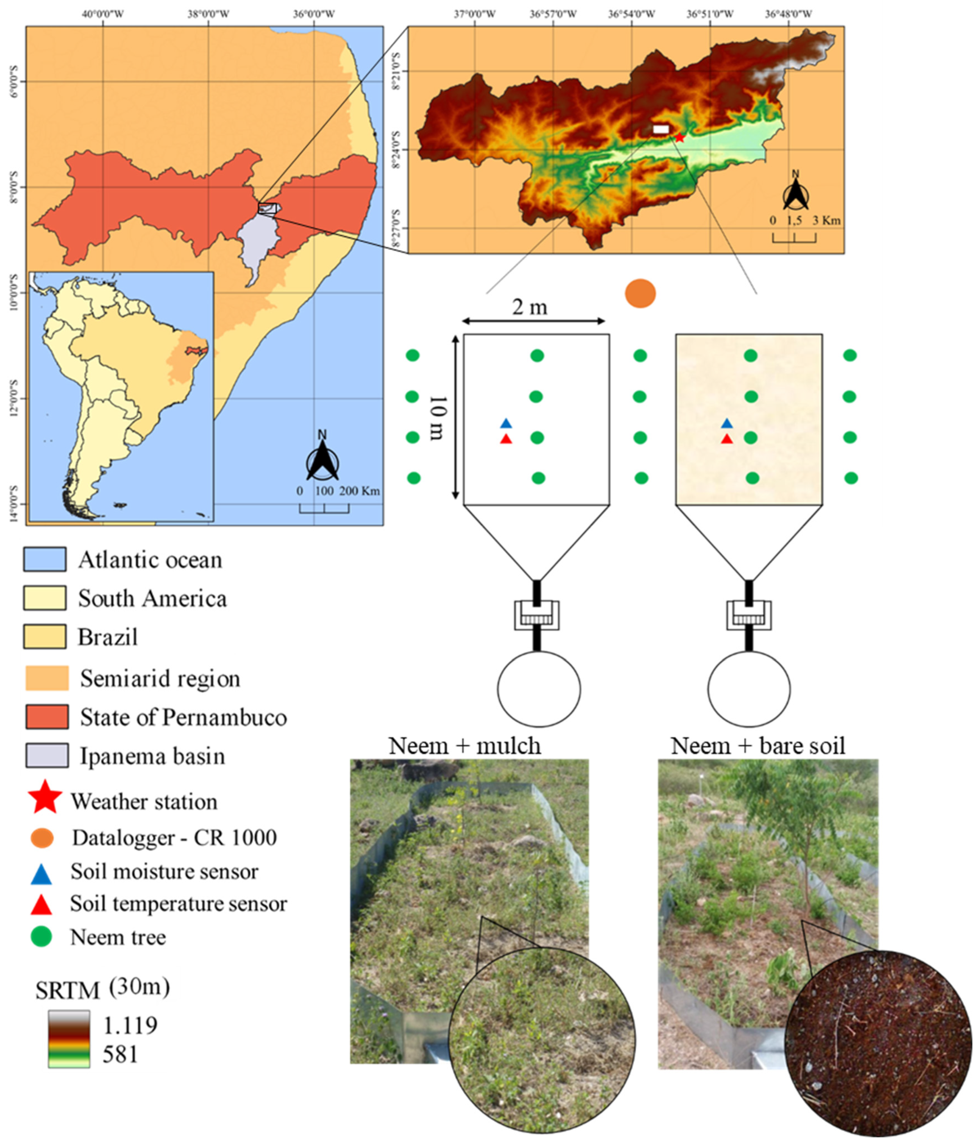
The research was conducted at the hillslope of the Mimoso Catchment, which is part of the Alto Ipanema Catchment in the Brazilian semiarid region of Pernambuco State, as seen in Figure 1. Two erosion plots, each measuring 20 m2 (2 × 10 m) with the longest side running along the slope, were installed in an area of 0.7 hectares.

Figure 1.
Location of the experimental area in the Alto Ipanema basin in the state of Pernambuco, Brazil, and Shuttle Radar Topography Mission (SRTM) with the hypsometry; sketches and photographs of two erosion plots and treatments in the studied area: Neem + mulch and Neem + bare soil.
The plots were placed on a longitudinal slope of 10%, and the following treatments were applied to each of them: BS—non-conventional perennial oilseed Neem (Azadirachta indica A. Juss) cultivated under bare soil conditions; M—Neem cultivated with coconut powder (Cocos nucifera L.), with a cover density of 8 t ha−1 (Figure 1). The transplantation of Neem species took place in May 2015, with plants spaced 6 m from each other. One and a half years after transplanting, the morphological characteristics of the species were monitored monthly, as follows: plant height (PH in m), obtained by measuring between the base of the stem and its apex, using a measuring tape, and the diameter of the stem (DC in mm), determined at the base of the plant at a height of 0.15 m, using a digital caliper. At the downstream end of each plot, 500 l reservoirs were installed to collect runoff and sediment transport (data not included in the scope of this study).
The soil in the study area, as described in detail in [4], was classified as a Regolith Neosol, with a relatively shallow depth of ~0.85 m and a sandy loam texture. According to the Köppen classification, the climate of the region is BSh (hot semiarid), with an average annual precipitation of ~686 mm, a reference potential evapotranspiration of approximately 2000 mm, and a mean temperature of ~23 °C [4]. Natural vegetation (Caatinga Biome) has been suppressed with time, and erosion processes have occurred at the hillslopes, thus requiring the adoption of conservation techniques to control overland flow and sedimentation down the alluvial valley. More information about the downslope valley can be found in Lima et al. [8].
The experiment was conducted from January 1st to December 31st, 2017. The meteorological data for the duration of the experiment was obtained from an automated weather station (Campbell Scientific) located nearby, providing records of air temperature, relative humidity, global solar radiation, atmospheric pressure, wind speed and direction, and rainfall. The minimum and maximum temperatures and relative humidity were used to calculate the reference evapotranspiration (ET0) [37]. The Climatological Water Balance was calculated using the methodology proposed by Thornthwaite and Mather [38]. Campbell CS-616 soil moisture probes were installed in the vertical position at 0.10–0.20 m, and temperature probes were inserted at 0.20 m soil depth and connected to the CR1000 datalogger for the detailed monitoring of wetting and drying processes in the soil profile for each treatment.
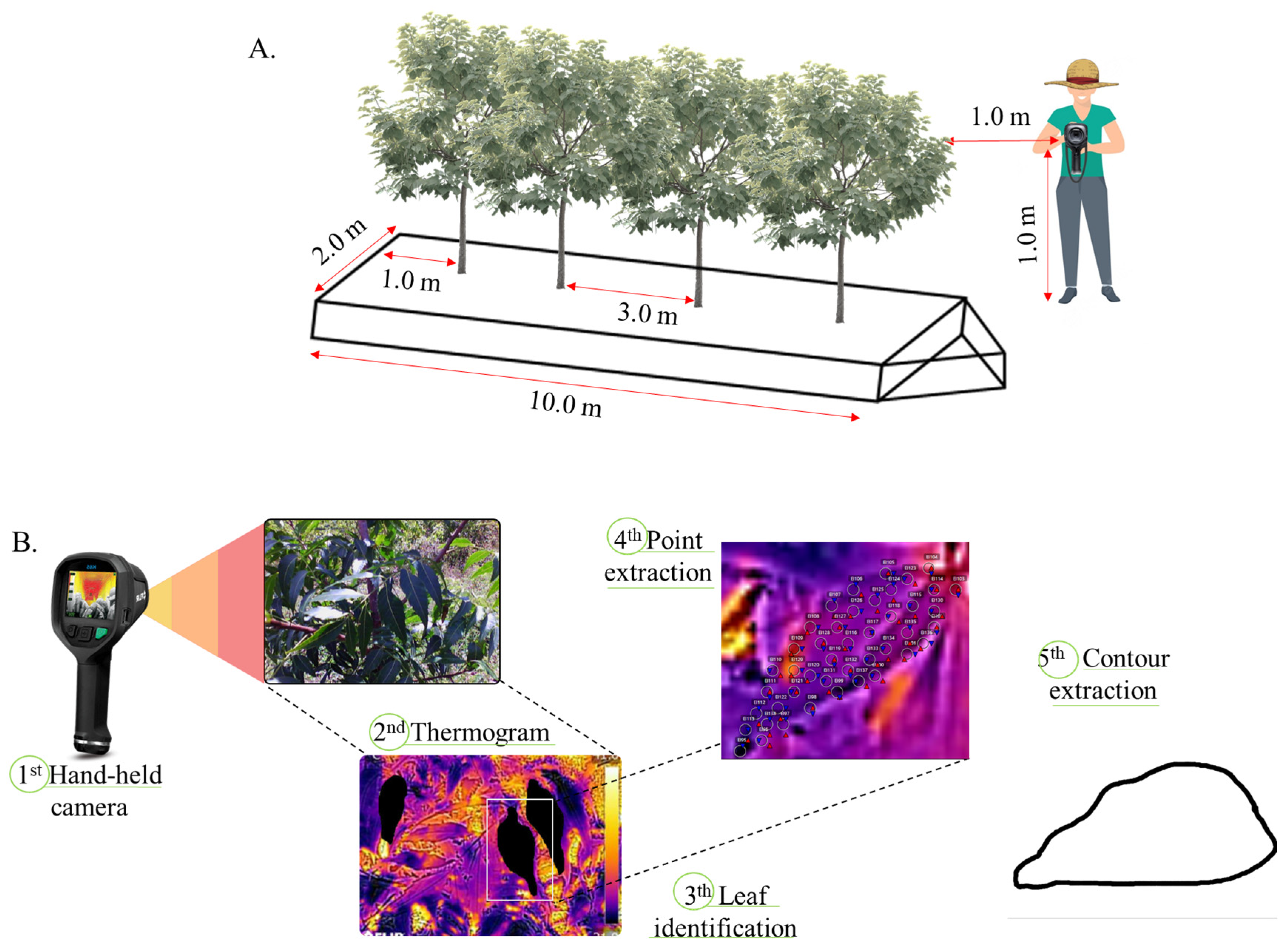
2.2. Image Acquisition and Analysis
Forty-eight thermal images of Neem leaves were obtained using a portable hand-held infrared camera (Model E6 from Flir Systems) with an IR pixel resolution of 19,200 (160 × 120), a field of view of 45° × 34° and a thermal sensitivity of <0.06 °C. The images were always recorded at 10:00 am, with the camera positioned at 1.0 m height from soil surface and 1.0 from the plant, as can been seen in Figure 2. Images were taken for the twelve months of 2017 for each treatment condition, and to develop the thermal image processing algorithm, we used Python with the OpenCV library, through the PyCharm interface. The purpose was to enhance canopy visibility and extract leaf contours. Filtering and thresholding techniques were applied to reduce noise and emphasize the canopy. The cv2.findContours() function identified leaf edges, and approxPolyDP extracted key points for further analysis (Figure 2B). For the detection of leaf thermal behavior, a script in Python language was elaborated for the detection and extraction of points and the contour of leaves representative of the canopy (e.g., less wind influence, absence of shading, and ease of liming by the algorithm), for each treatment.

Figure 2.
Sketch of the procedure of capturing thermograms (A); processing images and extracting representative grids and contour from sampled leaves (B).
2.3. Water Stress Indicator
The canopy surface temperature data at the pixel scale obtained from thermal images were used together with the air temperature to calculate the daily water stress index, according to the equation proposed by Jackson et al. [39] (Equation (1)):
where: DWSI—daily water stress index (°C); TL—leaf surface temperature collected by the thermal camera (°C); TA—air temperature measured by the meteorological station at the time when the photos were taken (°C).
2.4. Statistical and Geostatistical Analysis
A statistical analysis was conducted to assess the significance of the variation in water status under different soil cover conditions. Spearman’s correlation coefficients among air temperature, DWSI, leaf temperature, rainfall, and soil moisture were calculated over the studied period. Multivariate principal component analysis (PCA) was applied to identify the most important variables related to water stress, soil moisture, air temperature, and soil temperature variability.
The data were submitted to descriptive statistical analysis. The coefficient of variation (CV) was categorized according to Warrick and Nielsen [40] criteria, with values below 12% classified as low, values between 12% and 24% classified as medium, and values above 24% classified as high. The Kolmogorov–Smirnov (KS) normality test (p ≤ 0.01) was also applied to verify whether the data had a normal distribution. Trend analysis was performed by estimating the trend surface using a quadratic polynomial function and examining the coefficients of determination obtained. Trends were considered to exist for R2 values greater than or equal to 0.7. In such cases, residual values from the detrended data were adopted for the spatial analysis.
For the geostatistical analysis, the GEOEAS software version 1.2.1 [41] was utilized to detect patterns of the spatiotemporal variability and spatial correlation of DWSI for separate leaves for each plant evaluated, under two different soil cover conditions, for the months of March, May, and September, considering the significant variations in climatic conditions. The geostatistical analysis was conducted by calculating the classical semivariance (Equation (2)), which estimates the structure and spatial association between pairs of observations, at the pixel scale.
where is the estimated value of the experimental semivariance of the data; and are the observed values of the regionalized variable; and is the number of pairs of measured values, separated by a distance h.
Semivariance theoretical fits were tested for the Gaussian, Spherical, and Exponential models, and the parameters (nugget effect), (sill), and a (the range of spatial dependence) were estimated.
The degree of spatial dependence (DSD) was assessed based on the methodology proposed by Cambardella et al. [42], which uses the relationship between the nugget effect and the sill of the adjusted semivariogram, classifying the spatial dependence as strong, moderate, or weak, as observed in Equation (3). Values below 25% are characterized by strong spatial dependence, values between 25% and 75% are considered moderate, while values above 75% indicate weak spatial dependence.
The best models were selected by analyzing the coefficient of determination (R2) and performing cross-validation using leave-one-out cross-validation [43], assuming a mean error close to zero and a standard deviation close to one.
After modeling the semivariograms, the values were interpolated at non-sampled sites using kriging (K). This technique uses both correlation with auxiliary maps and spatial correlation, where the drift (or trend) is modeled as a function of coordinates. The sequential Gaussian simulation (SGS) algorithm randomly selects a simulated value at each location from an estimated conditional cumulative distribution function. The distribution function is determined by the mean and variance of the kriging calculated from neighborhood information. Running the SGS requires transforming the original data into a Gaussian distribution, which is accomplished by transforming the normal score into (Equation (4)).
The cumulative density function is characterized by the mean and covariance, assuming a random Gaussian field. Repeating these sequential steps with different random paths can provide various runs of the spatial distribution. In this study, to obtain an accurate probability calculation, the SGS algorithm was conducted for one hundred runs using the GS+ software version 7.1, following Sousa et al.’s [44] recommendation.
After modeling the semivariograms, the values were interpolated using ordinary kriging, to characterize the leaf surface of the plants studied, in three different months. The SURFER version 9 software was used to make the kriging maps [45].
3. Results
3.1. Changes in Soil Moisture and Climatic Conditions
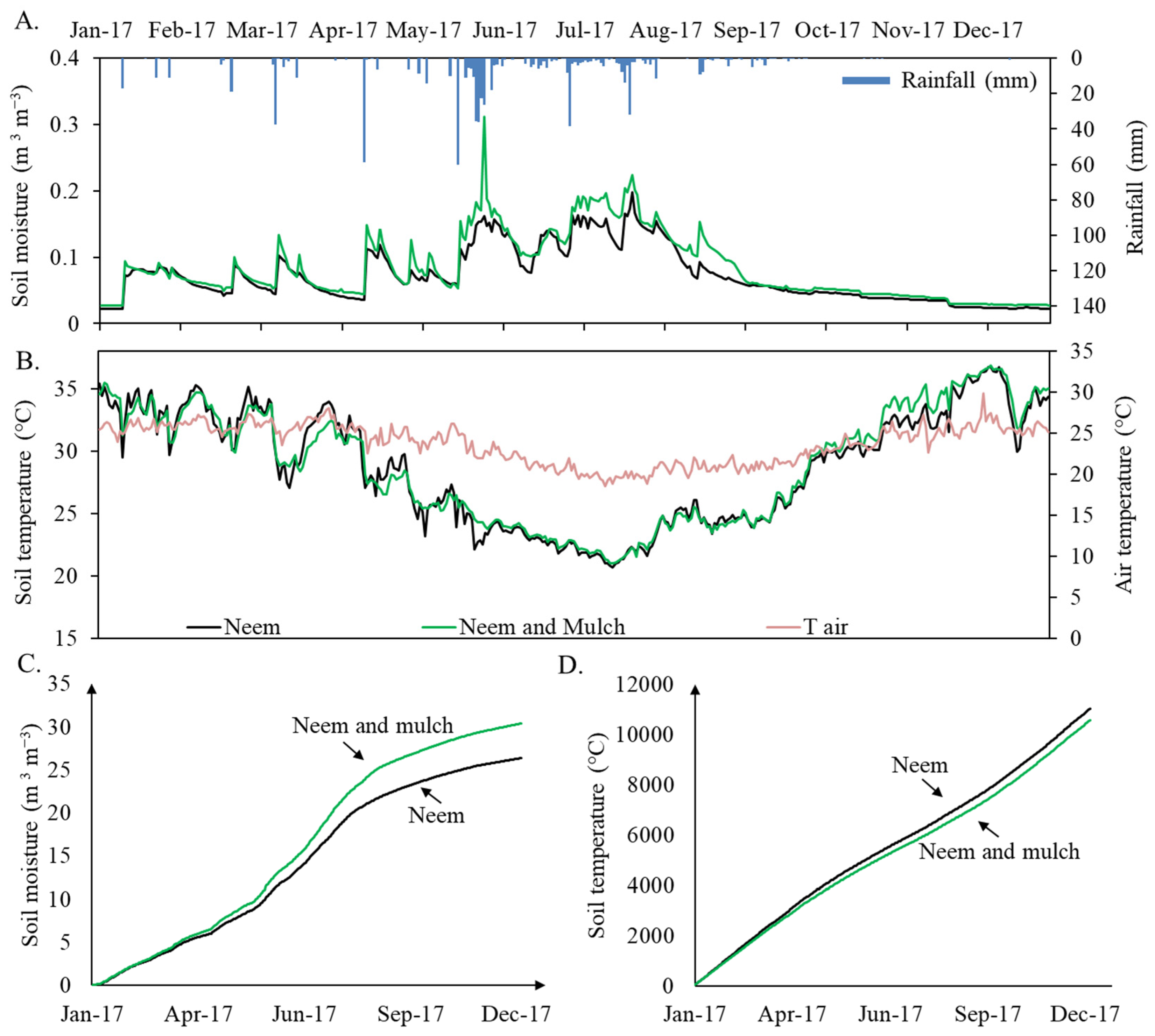
Soil surface temperature and moisture, for the bare soil and mulch treatments, including air temperature and rainfall variations in time are plotted in Figure 3. In general, 2017 could be classified as water-scarce, with a total of 50 rainfall events throughout the year. The highest precipitation depth was recorded in May with 266 mm, which constituted 35% of the total annual rainfall. The single highest rainfall event of that month was 60 mm. The months of April, June, and July presented rainfall amounts higher than 90 mm, while February, March, September, October, and December all had less than 30 mm. No rainfall was recorded in November.
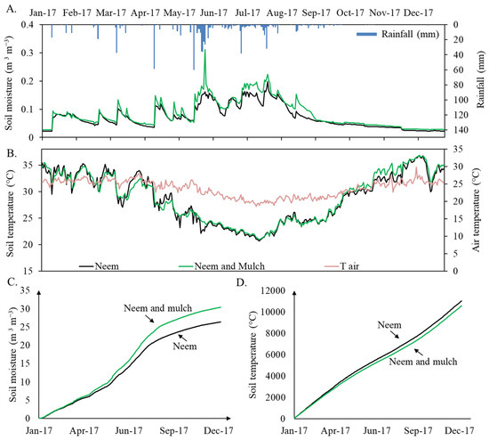
Figure 3.
Daily time series of soil moisture and rainfall (A), air and soil temperature (B), accumulated soil moisture (C), and accumulated soil temperature (D) at the two plots in 2017: Neem (bare soil in black) and Neem with mulch cover (in green).
During the period evaluated, the average air temperature was 23.70 °C ± 2.37, with a maximum of 29.84 °C Day−1 and a minimum of 18.54 °C Day−1. Regarding soil temperature, a temporal variation was observed among the seasons, with higher values in December (bare soil condition: 35.58 ± 1.89 °C; mulch soil condition: 35.13 ± 1.49 °C) and lower values in May (bare soil condition: 25.43 ± 1.41 °C; mulch soil condition: 24.97 ± 0.79 °C), with a maximum of 36 °C and a minimum of 20.1 °C for the treatment with mulch, and 37.80 °C and 21.50 °C for the treatment without mulch. In general, the use of the cover reduced the maximum temperature by 1.8 degrees and the variation by 0.4 °C. Additionally, when analyzing the seasonal changes in soil moisture levels between the two soil cover treatments, higher soil moisture was observed during the rainy season (May to August) for the treatment with mulch (0.14 ± 0.02), which contributed to retain water, reducing evaporation and thus increasing soil moisture in 18%. In general, the cumulative evolution of soil moisture (Figure 3C) and temperature (Figure 3D) shows significant differences when comparing the two treatments. For the bare soil condition, a decrease of 5% in cumulative soil moisture and an increase of ~5% in temperature in comparison to the mulch application plot were observed in the course of 2017.
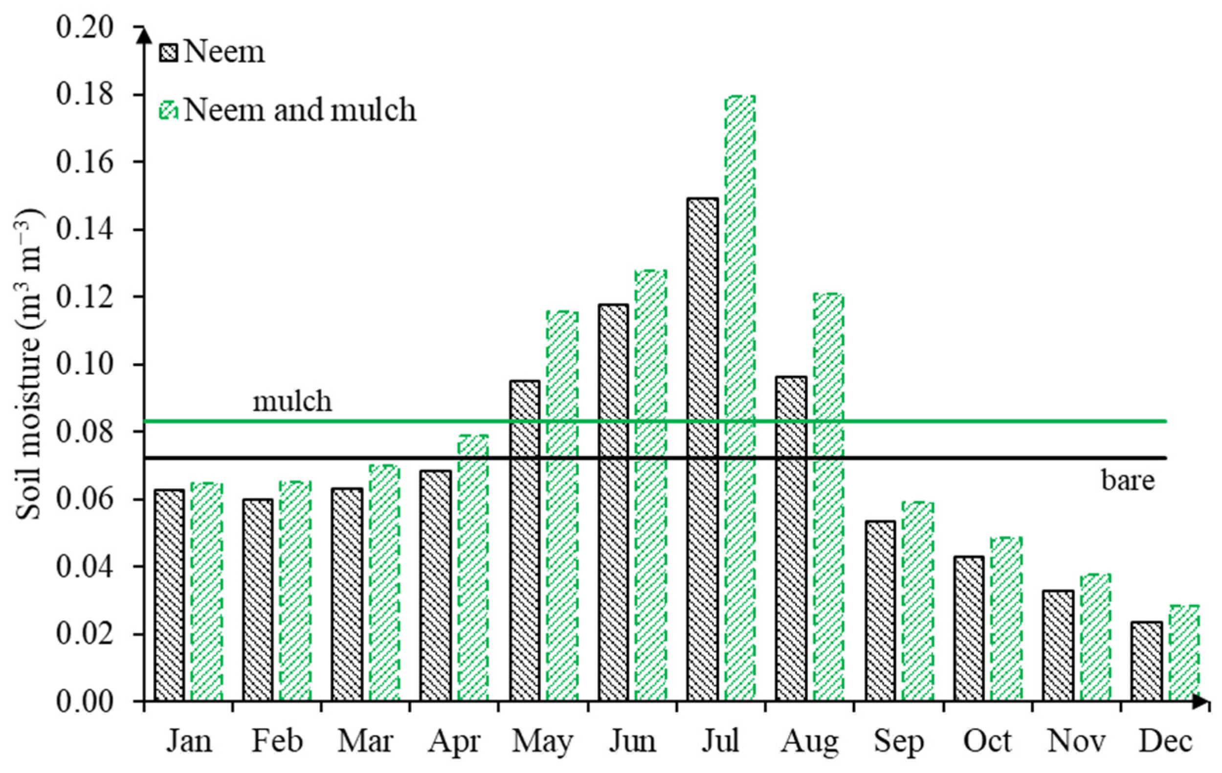
Figure 4 compares the monthly variation of soil moisture in the course of the whole year for both soil cover conditions. Higher soil moisture contents along hillslopes not only contribute to crop development, but also control overland flow and enhance subsurface flow, which is of the upmost relevance for semiarid areas [46]. Furthermore, soil moisture also has a direct influence on soil microbiology, mineralization, and the emissions of gasses into the atmosphere (e.g., carbon dioxide CO2 and Nitrogen N2 that are influenced by soil humidity and temperature, for example), among others.
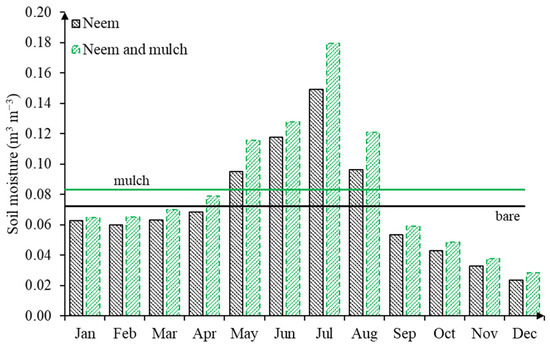
Figure 4.
Monthly soil moisture variation for both soil cover conditions (bare in black and mulch in green), in the course of 2017.
Studies have suggested that the mulch cover was efficient in soil water retention compared to uncovered soils, especially for the wet period when moisture levels ranging from 0.13 to 0.15 m3 m−3 were observed, with humidity in the dry months being 17% higher than the humidity in the bare soil treatment. For the period between April and August, the average of soil moisture exceeds the annual mean of 0.083 ± 0.02 m3 m−3 for the mulch soil cover condition and 0.07 ± 0.04 m3 m−3 for bare soil, as a result of rainfall events. In the absence of precipitation, the mulch cover works as an alternative soil protection technique.
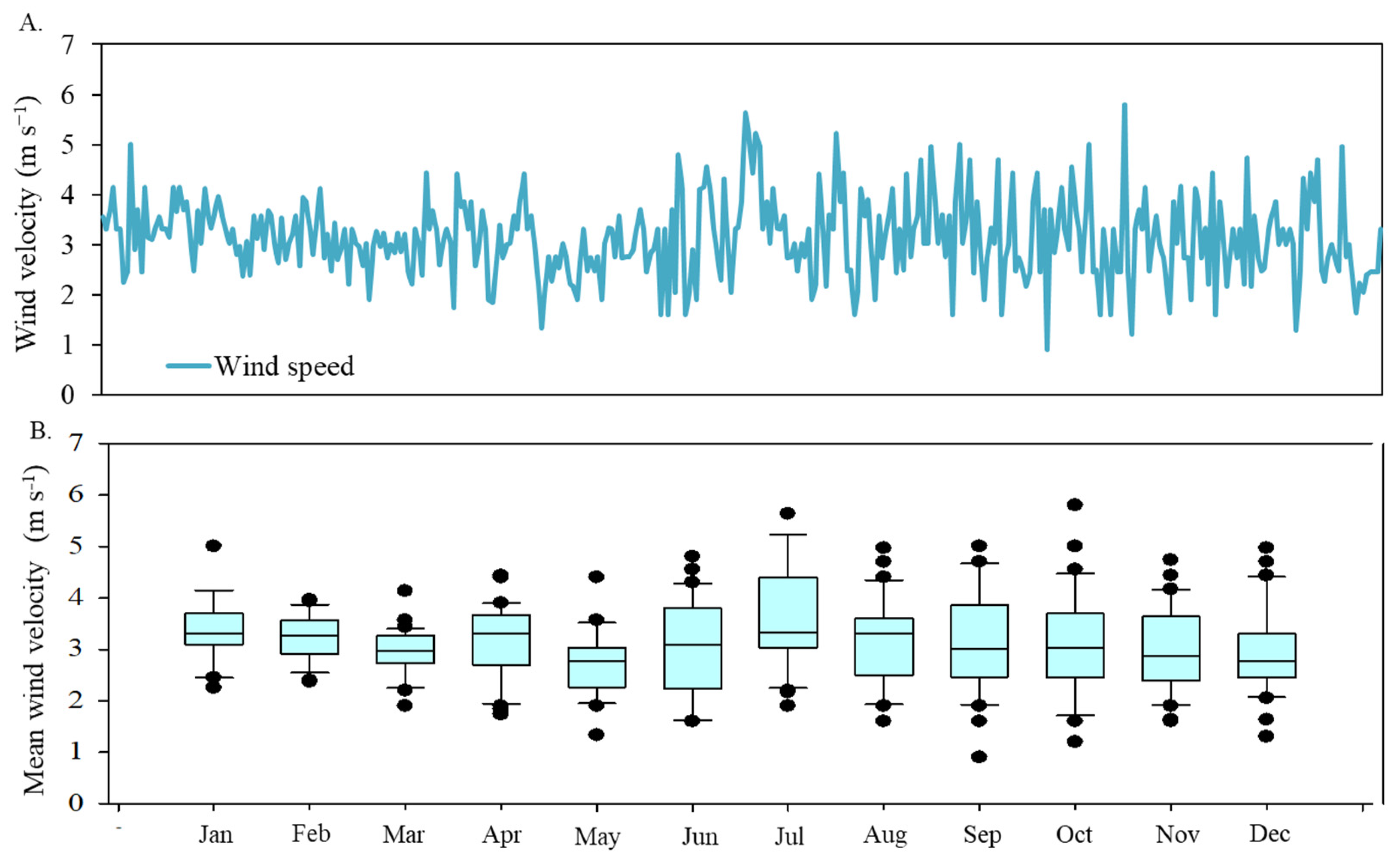
Wind velocity is another critical factor influencing plant water stress. Figure 5 illustrates the diary fluctuation of mean wind velocity from January to December 2017. The wind velocity values exhibited an average of 3.13 m s−1, with a standard deviation of 0.80 m s−1.
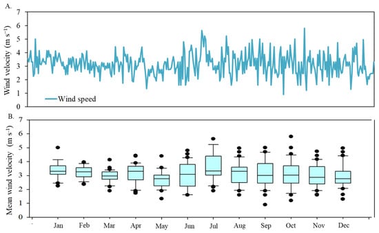
Figure 5.
Temporal distribution of mean wind velocity (A), in meters per second, in 2017 and box plot of monthly values (B).
The average wind speeds ranged from 2.94 m s−1 in December to 3.60 m s−1 in July. The period from June to November experienced the highest variability. Lower temperature periods, typically during or immediately after rainy months, also correspond to higher wind speeds.
3.2. Daily Water Stress Index
Table 1 presents the accumulated rainfall of 15 days before the monitoring date, and daily values for rainfall, evapotranspiration, wind speed, and temperature corresponding to the day of the field measurement. It also includes a mean leaf temperature measured by a thermal camera and the mean daily water stress index, measured at 40 pixels. The capture of thermal images and data in January, April, May, and July occurred on rainy days with an accumulated rainfall of 11.2, 2.6, 8.6, and 0.4 mm, respectively.

Table 1.
Daily values of rainfall, evapotranspiration, air and leaf temperature, and stress index for 2017, where BS—bare soil conditions and M—mulch soil cover conditions.
The minimal daily air temperature for the monitored days was 20.1 °C (in July) and the maximum 26.4 °C (in November). Regarding daily leaf temperature, the minimum value was recorded in July (25.36 °C) and the maximum in January (47.35 °C) for bare soil conditions, presenting a reduction of 1.91 °C (7.5%) in July and 2.56 °C (5.4%) in January for mulch soil cover conditions. A significant difference in crop status between bare soil and mulch cover was observed, with the exception of January, March, and April. Such a result highlights the effectiveness of mulch in maintaining soil moisture from previous rainfall events, as is also shown in Figure 3. Generally, the highest levels of water stress were recorded in January and December 2017 due to high evapotranspiration rates and low antecedent rainfall.
The influence of daily evapotranspiration is observed, as a response to air temperature, together with the absence or presence of rain in the daily water status dynamics. Plant height, stalk diameter, leaf temperature, daily water stress, and water balance measured during the experimental time can be observed in Figure 6.
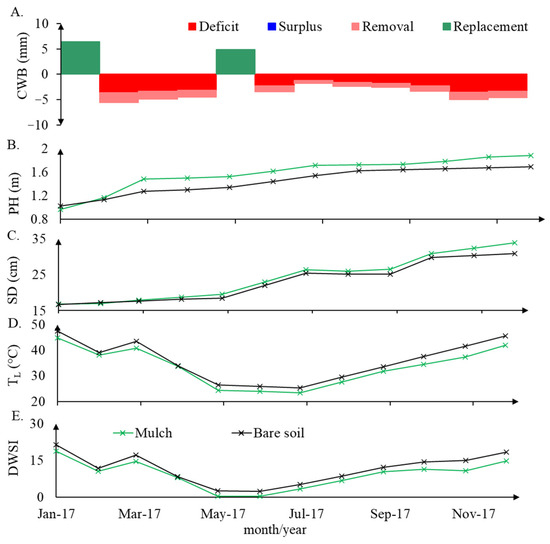
Figure 6.
Monthly water balance (CWB) (A), monthly average plant height (PH) (B), stem diameter (SD) (C), leaf temperature (TL) (D), and DWSI (E) under bare soil and mulch soil cover conditions.
A long water deficit period was observed from February to April and from June to December, when the reference evapotranspiration was higher than rainfall. For January and May, when there was no water surplus, rainfall was higher than the reference evapotranspiration; however, there was still available soil water content because of rainfall antecedent conditions. There is a statistically significant difference in the height of plants and stem diameter between January and December 2017, demonstrating the growth that resulted from the water replenishment events in January and May.
3.3. Relationships between Thermal Indices and Meteorological Parameters
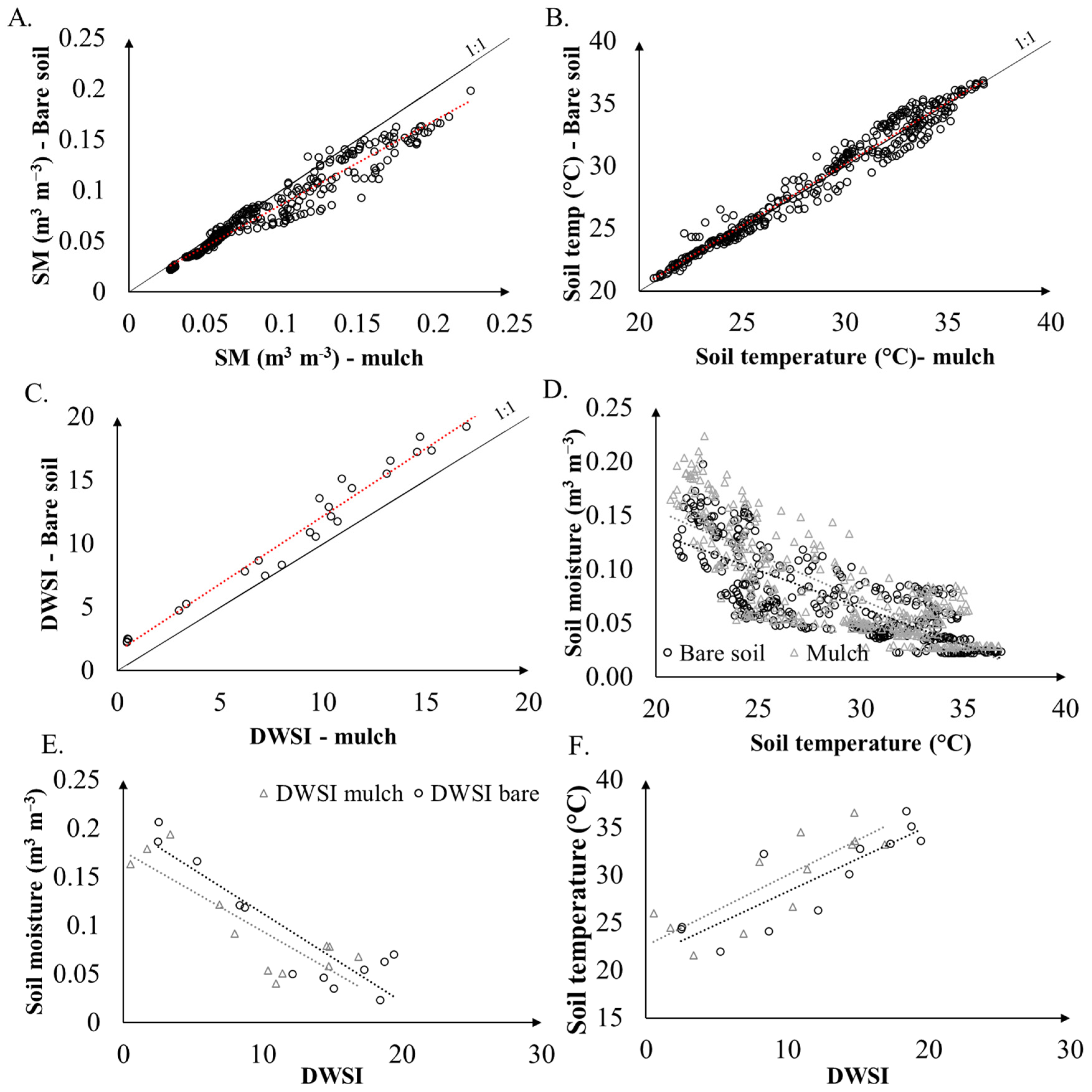
Figure 7A–C exhibits the relationship between soil moisture, soil temperature, and daily water status, for bare and mulch cover conditions. The lowest data dispersions and strong correlations between soil treatments occurred for values smaller than 0.1 m3 m−3, since the higher the soil moisture, the lower the daily thermal amplitude, given the high specific heat of water [4]. Besides that, some differences in soil moisture occurred at the beginning of the rain season, or after periods of intermittency [47]. According to Figure 7, a strong relation is observed between both conditions of soil temperature, with slopes close to 1.
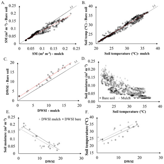
Figure 7.
Plots of soil moisture (A), soil temperature (B), DWSI (C), soil moisture and soil temperature (D), soil moisture and DWSI (E), and soil temperature and DWSI (F), for mulch and bare soil cover conditions. Dashed lines represent regression lines. The full line represents the 1:1 line.
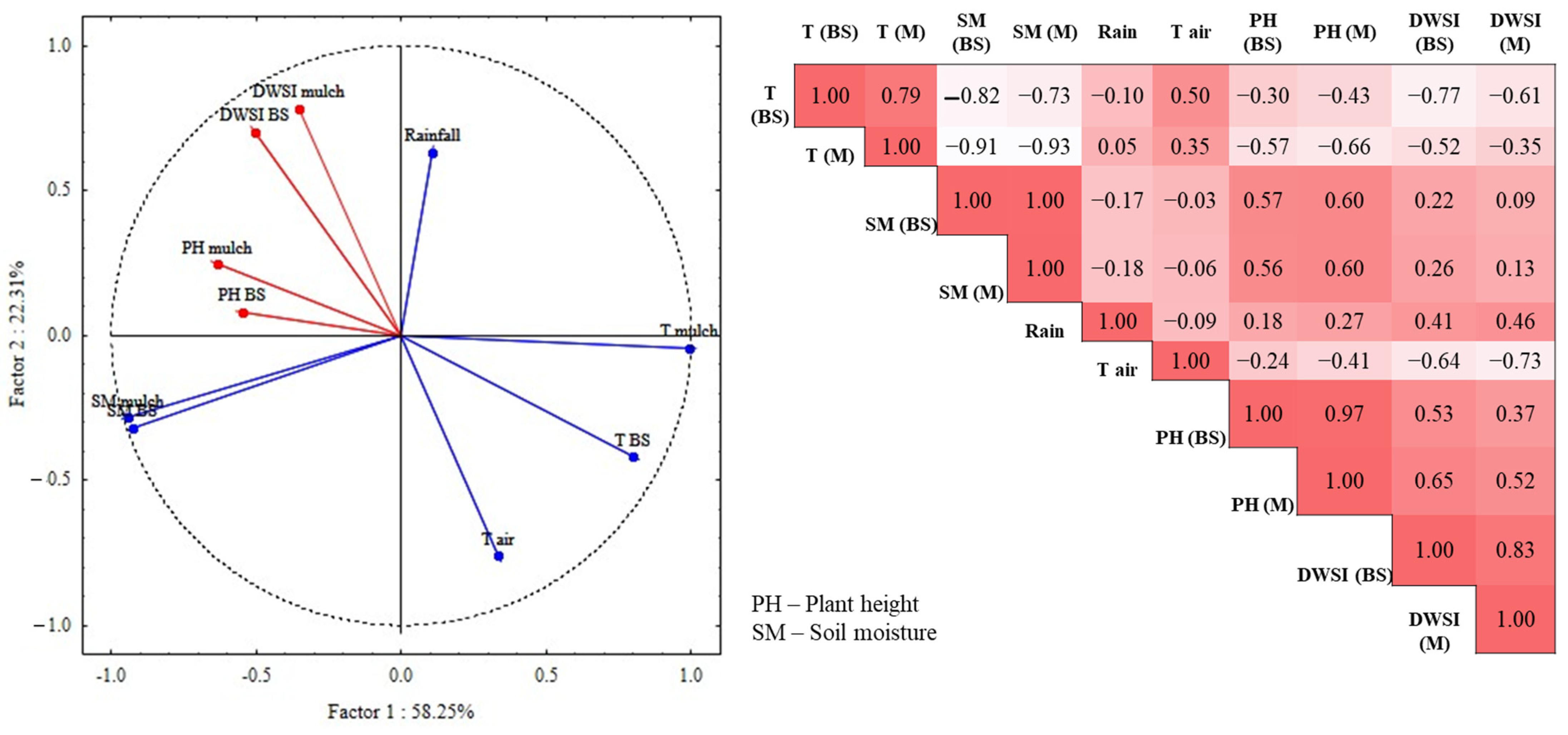
The correlation analysis of DWSI under bare and mulch soil conditions with soil moisture and soil temperature show that the plots managed under a conservation method presented a reduction in the water stress index as they showed a higher moisture content, and, additionally, a lower soil temperature. The plants that were grown with mulch cover showed better development than those without soil cover. To validate the previous results and to evaluate the effects of temperature and soil moisture on plant development, principal component analysis (PCA) was applied to the original matrix of temperature and soil moisture, with plant height and DWSI as supplementary variables. The plot of the PCA for the soil parameters and plant conditions is shown in Figure 8.
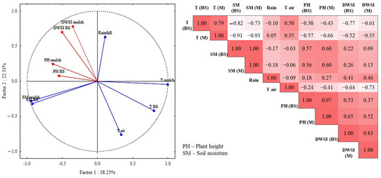
Figure 8.
Principal component analysis, plotting of scores of the first two principal components, and Spearman’s correlation matrix.
The main components, Factor1 and Factor2, explained 74.56% of the total variance, with Factor1 notably explaining 58.25% of the total data variance. In this PCA, it is possible to observed that the variables related to the temperature of soil under mulch and bare soil conditions, and air temperature were grouped and presented loads of 0.79, 0.99, and 0.33, respectively, denoting a strong negative correlation inversely influenced by soil moisture and rainfall. The stress indicator and the plant height showed a negative correlation with temperature for both soil cover conditions. In the correlation matrix, plant height (PH) and DWSI showed strong correlations (p < 0.001) for mulch treatment (0.85) and bare soil.
3.4. Plant Canopy Status Mapping
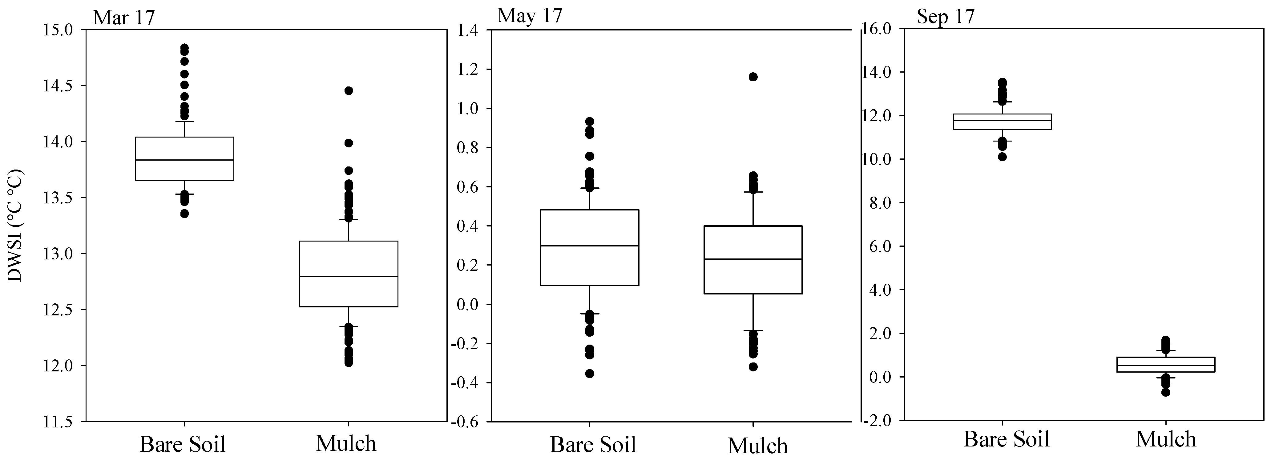
After obtaining the reference temperatures necessary for calculating the DWSI, a spatial representation of the index was created across six representative leaves. The months of March, May, and September were chosen according to the quality of images, weather conditions on the day of monitoring, and the significance of results for leaf comparison between treatments. The choice of leaves was made considering the best-defined contours within the canopy. Figure 9 shows the box plot of the stress index recorded for both conditions of soil cover, for March, May, and September. The water stress for March ranged between 11 and 15 for bare soil, and between 11.3 and 11.9 for mulch cover conditions. In May, the lowest stress values were identified, with a minimum of −0.4 and −0.3 and a maximum of 1.2 and 1.6, for bare soil and mulch, respectively. Although low DWSI values were detected for the bare soil condition, a more asymmetric distribution with a smaller presence of extreme values was detected in the mulch soil cover condition. In September, the contrast between treatments is evident, with minimum values of 10 and −1.6 and maximum values of 14 and 2, respectively, for the bare soil and mulch treatments. An asymmetry in the data distribution is also observed for the bare soil condition.

Figure 9.
Box plot of daily water stress index for March, May, and September, of mulching treatment and bare soil, for three different leaves.
The DWSI for May presented a smaller variation, with the coefficient of variation (CV < 15%) indicating low variability, according to Warrick and Nielsen [40], and lower standard deviation values, followed by September and March. All plant samples presented normality at 5% probability, allowing the researchers to obtain the parameters of theoretical semivariograms from the experimental data (Table 2). The minimum number of pairs for the experimental semivariograms was 40, based on pixel meshes comprising at least 32 elements.
Table 2.
Parameters of the theoretical models for the semivariance of the DWSI in each leaf sampled in March, May, and September.
The DWSI showed spatial dependence which was best described by a Gaussian model for both treatments in all months evaluated. The stress index presented different ranges of spatial dependence for both treatments, with a minimum value of 43 mm and a maximum of 92 mm, referring to March, for both soil conditions, 43 and 185 mm, referring to May, and 46 and 133, referring to September, respectively.
The relationship between the nugget effect and the sill ranged from 0.7% (May–mulch) to 33% (May–bare soil), indicating a strong and medium spatial dependence for the analyzed months, according to the classification of Cambardella et al. [42]. In general, the plants cultivated under the mulch soil cover condition present a strong spatial dependence. The coefficients of determination (R2) for the fitted models were moderate to high, with a minimum of 0.8 and a maximum of 1, and all the semivariograms were cross-validated based on leave-one-out cross-validation [43], yielding residues with averages between −0.001 and 0.013, and standard deviations between 1.004 and 1.006.
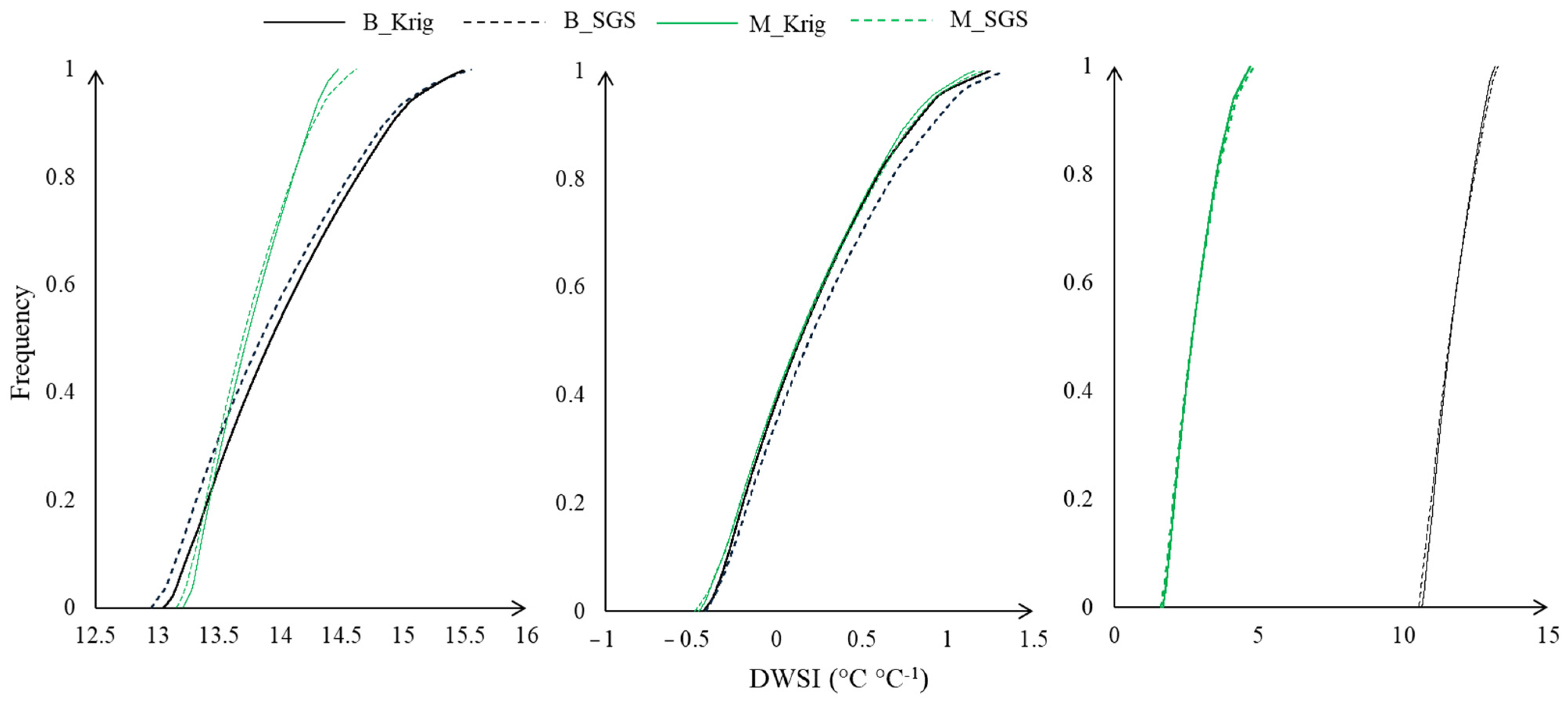
The fitted models were used for mapping, employing both ordinary kriging (OK) and sequential Gaussian simulation (SGS) techniques, and their respective standard deviations of the estimates/leaf water status maps from plants grown for the moths March, May, and September cultivated under bare soil and mulch soil cover conditions (Figure 10). By employing the sequential Gaussian simulation (SGS) technique, the fitted models were also used to produce maps of the DWSI with 300 realizations, as shown in Figure 10. The scale of DWSI for March, May, and September varied from 12 to 16 °C, −1 to 2 °C, and −1 to 15 °C, respectively. The SGS provided an accurate reproduction of the spatial variability pattern compared to kriging.
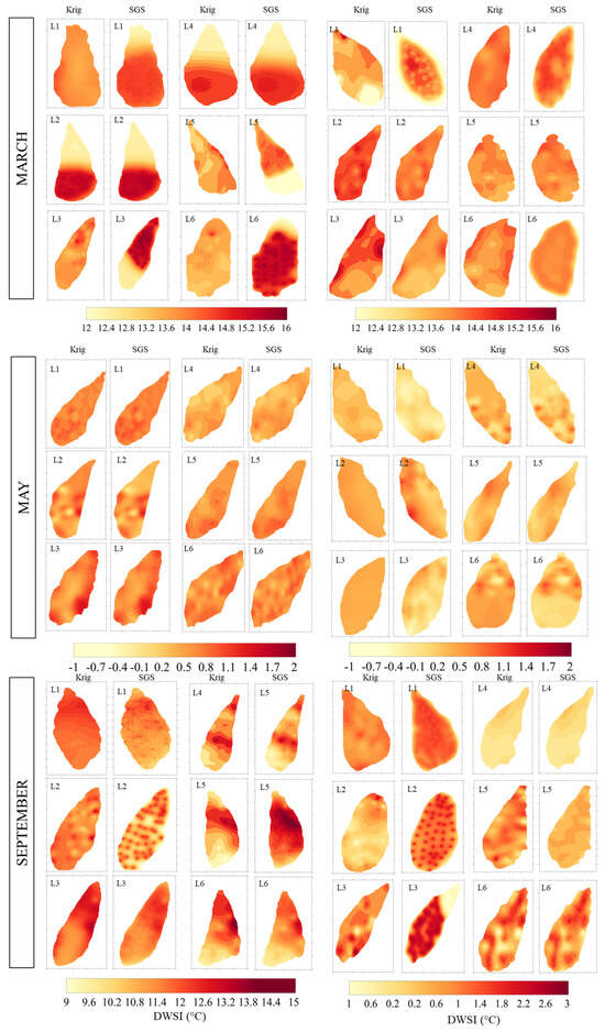
Figure 10.
Kriging maps for surface temperature referring to representative leaves for March, May, and September, considering bare soil and mulch cover conditions.
A distinction can be seen between maps, with higher occurrences of red areas representing higher stress due to temperature and climatic effects, indicating lower water status. Some negative values were also found, indicating that the plants were not under any water stress in any part of their leaves, especially in May due to the rainfall and in September due to the mulch condition, showing that mulch facilitates a more even distribution of water and mitigates external effects on the leaf surface, such as wind speed.
We generated cumulative frequency curves based on temperatures extracted from thermal images and air temperature using the kriging and SGS methods (Figure 11). Overall, the curves exhibited similar trends across treatments. However, the DWSI ranges varied according to soil moisture levels and rainfall availability. In March, the DWSI ranged from 12.5 to 16, while in May, it ranged from −1 to 1.5. The most significant variation occurred in September, ranging from −2 to 15. This wide range in September can be attributed to the effective use of mulch cover, which mitigates climatic effects on plants and reduces stress. Specifically, the mulch condition produced a DWSI distribution between −2 and 4, whereas the DWSI of the bare soil condition ranged between 10 and 13.
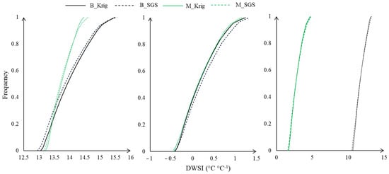
Figure 11.
The canopy DWSI cumulative frequency curves for plants evaluated in the respective months (March, May, and September) under bare soil and mulch conditions.
When evaluating the average DWSI across months and soil cover conditions (Table 3), a notable difference emerges compared to the previously presented values (Table 1). It is important to note that the earlier values were calculated based on a single plant sample point, whereas the extraction of leaf temperatures represents the plant’s actual temperature more critically and rigorously. Additionally, it is observed that mulch application effectively contributed to reduce water stress and intrafoliar temperature variation, indicating a more uniform stomatal behavior.
Table 3.
Parameters of the theoretical models for the semivariance of the DWSI in each leaf sampled in March, May, and September.
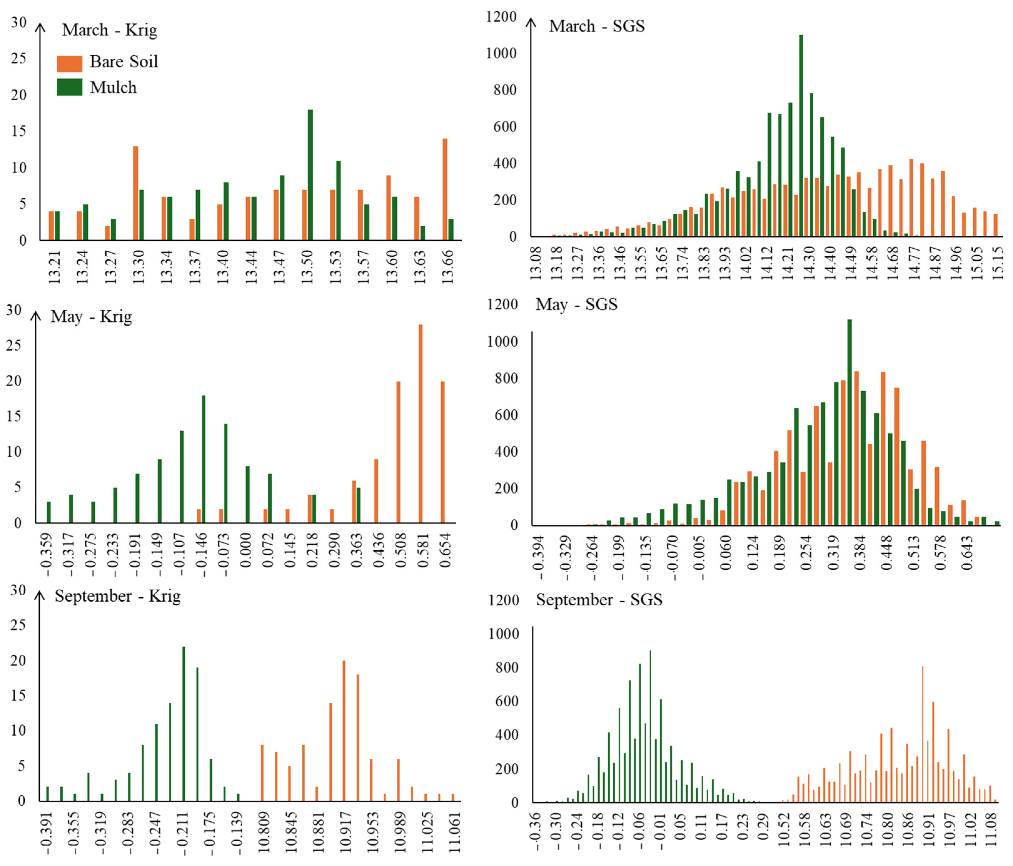
Figure 12 presents the histogram of the DWSI distribution of the kriging (Krig) and sequential Gaussian simulation (SGS) methods. When comparing the histograms of Krig and SGS results, it is notably that the SGS realization histogram is similar to the histogram of the Krig results. However, SGS provides additional information about the uncertainty in the spatial distribution, which is not captured by a smoothed Krig estimate.

Figure 12.
Histograms of the distribution of DWSI for the months of March, May, and September, under mulch and bare soil conditions, following mapping via kriging and SGS techniques.
By analyzing the histograms, it is possible to detect greater symmetry in the distribution of DWSI in plants with lower stress levels, as it is an indicator of plant water comfort. The plants that received conservation management exhibited more symmetrical distributions, indicating better adaptation and a more balanced state of health.
4. Discussion
It can be observed that air temperature followed the climatic seasonality of the semiarid region (Figure 3), with higher values in the dry season and lower values in the rainy season, consistent with the temperature dynamics observed by Lima et al. [8] while assessing climatic trends in the same alluvial valley as the present study. In general, leaf temperatures were lower during periods with lower air temperatures, consequently showing lower levels of water stress, in line with the findings of King et al. [48]. The authors highlight that canopy temperature increases when solar radiation is absorbed and decreases when water evaporates (transpiration) within the leaf structure. A plant canopy experiencing water stress will reduce transpiration and exhibit a higher temperature compared to a canopy without stress.
Wind speed patterns also exhibited a distribution of monthly variation sensitive to the presence of rain events (Figure 5). As highlighted by Miri et al. [49], wind speed is a significant factor contributing to plant water stress by increasing transpiration and water loss from leaves. Higher wind speeds lead to greater wind stress and water loss from plants. The sensitivity of plant water stress to meteorological factors was also observed by de Andrade et al. [35], where the authors highlighted the monthly variation in air temperature and canopy temperature patterns between the rainy and dry periods, mainly in the nocturnal period, corroborating the DWSI variations found (Table 1).
Although canopy temperature and the DWSI are closely related to meteorological conditions and cumulative water balance (Figure 6), Bo et al. [10] emphasize that the soil cover condition also influences canopy temperature and consequently water stress. The authors evaluated, in a two-year field experiment, the cultivation of corn under different mulching conditions in northwest China and found positive effects of plastic mulching on canopy temperature and the crop water stress index (CWSI), consistent with the results found in the present study. As seen in the soil moisture temporal dynamics in Figure 3 and Figure 4, mulching proved to be an efficient alternative for soil protection. Moreover, the correlations between soil moisture and temperature, and the daily water stress index, for mulch and bare soil conditions (Figure 7A–C) demonstrate that the higher the soil moisture, the lower the thermal amplitude. This reduction in thermal amplitudes was also explained by de Lima et al. [50] in their study on the effects of mulching on soil temperature and moisture also in the Brazilian semiarid region, where mulching reduces soil surface temperature, acting as a buffer zone and dampening soil surface temperature fluctuations.
Positive correlations between soil moisture and the DWSI, as well as negative correlations between soil temperature and the DWSI, can be observed in Figure 7E,F. Akthar et al. [51] also reported significantly increased moisture retention and decreased soil temperature during warm periods with the application of wheat straw mulch in Northwest China, creating favorable conditions for soybean growth compared to non-mulch treatments. Additionally, Lopes et al. [52] monitored soil and water dynamics in twelve experimental plots across the same hydrological area with varying coverage treatments. They found that runoff behavior differed; natural cover produced the smallest runoff depth, while bare soil conditions resulted in the highest runoff.
The value of the DWSI (Table 1 and Table 3 and Figure 6) reflects the physiological characteristics of the plants in relation to the environment [24]. Hence, plant water status controls many physiological processes and crop productivity, associating a crop’s higher water stress with greater daily evapotranspiration, thus reflecting the biometric crop development [53]. Brunini and Turco [24] observed a decrease in productivity for sugarcane species as values exceeded 1.5. The greater water availability from intense rainfall events was found to be a mitigating factor of stress along the leaf surfaces. In Figure 8, it is possible to observe that plants with lower stress indices, promoted by the mulch condition, exhibited better growth in terms of both plant height and stem diameter. The changes in stem diameter have been closely linked to variations in the overall water content of the plant [53]. For this reason, several researchers have observed that leaf turgidity (LT) values can be a useful indicator of stress when soil water content is not severely depleted, and increases in LT have been observed to correlate with decreases in water potential. As plant growth is controlled by cell division, an insufficient amount of water reduces the division coefficient cell and the expansion of all cells, thereby preventing the proper vegetative growth of plants [22,54,55].
In order to effectively measure plant temperature and identify water stress conditions, Paulo et al. [56] emphasize that leaf temperature maps are validated by thermal images as an effective and practical alternative. In the DWSI distribution maps (Figure 10), higher values are observed at the leaf apex and outer areas, primarily affected by wind, as discussed earlier. These results demonstrate that using average leaf temperature data or considering only the highest marginal values or including very low marginal values may result in biased and unrealistic DWSI values and may not accurately reflect the plant’s water status. Therefore, the choice of TL statistics for DWSI calculation is relevant [15,22,28].
Moreover, Luan et al. [15] emphasize that the information of leaf temperature distribution can reflect the water status of the crop. The curves presented in Figure 11, depicting the DWSI calculated from the temperature distribution, exhibited similar trends among treatments; however, the ranges of leaf DWSI varied under different soil moisture conditions. Furthermore, conservation management proved effective in maintaining soil moisture and reducing water stress, as evidenced by the detailed analysis of the histograms (Figure 12). The coefficient of variation (Table 3) of the data was reduced by sequential Gaussian simulation compared to kriging, demonstrating the improvement of mapping through scenario repetition and lower uncertainty for the spatial distribution, as well as for representative leaves of the conservation treatment. This pattern was consistently observed across different monitoring periods, reinforcing the importance of sustainable agricultural practices for the resilience of crops in semiarid environments.
Additionally, SGS exhibited a class distribution five times larger than that of kriging mapping. This finding confirms the results of Bai et al. [57], who suggest that kriging can lead to a smoothing effect, resulting in an overestimation of small values and an underestimation of large values, thereby restricting its applicability to assess uncertainties in certain situations and lower scales.
Our results demonstrate the high potential of thermographic data to produce distributed crop water stress indices, which allowed for estimating and interpreting the plant’s water status, reducing associated errors through leaf geostatistical mapping. By identifying patterns of variation that reflect higher or lower stress indices, this method provides a non-destructive and quicker means of detection and monitoring of crop temperature variability.
5. Conclusions
We investigated the water stress on crops, which can severely disrupt crop growth and reduce yields, especially in semiarid regions. An accurate and prompt diagnosis of crop water stress is crucial. Infrared thermal imaging cameras were utilized to monitor the spatial distribution of canopy temperature (Tc), forming the basis of the daily water stress index (DWSI) calculation. The application of geostatistical techniques enabled stress indicator mapping at the leaf scale, with spherical and exponential models providing the best fit for both soil cover conditions.
In conclusion, the DWSI reflects changes in biometric indices, demonstrating high potential as an indicator of the relationship between plant and climatic variables measured on a daily basis. The results indicated that the highest levels of water stress were observed during the months with the highest air temperatures and no rainfall, especially at the apex of the leaf and close to the central veins, due to a negative water balance. Even under extreme drought conditions, mulching reduced Neem physiological water stress, leading to lower plant water stress, higher soil moisture content, and a negative skewness of temperature distribution.
Furthermore, the daily water stress index (DWSI) differs according to soil cover condition, evapotranspiration, and the sequence of rainfall events. The mulching effect during long dry periods, typical of semiarid regions, was essential for preserving soil moisture and promoting plant growth. Even in extreme cases of water scarcity, mulching reduced the physiological water stress of Neem, leading to decreased water stress and a reduced recession of soil moisture content, resulting in better biometric parameters.
Regarding the mapping of the stress index, the sequential Gaussian simulation method reduced temperature uncertainty and variation on the leaf surface. Our findings highlight that mapping the water stress index offers a robust framework for precise stress detection in agricultural and soil cover management in semiarid regions. Coupling thermography with geostatistical tools enabled a precise assessment of water stress index mean and variability for a resilient crop in semiarid Brazil. These findings underscore the impact of meteorological and planting conditions on leaf temperature and baseline water stress, which can be valuable for regional water resource managers in diagnosing crop water status more accurately.
Author Contributions
Conceptualization, T.A.B.A., A.A.A.M. and J.L.M.P.d.L.; methodology, T.A.B.A., J.L.M.P.d.L., J.R.L.d.S. and R.A.B.d.S.; software, T.A.B.A., R.A.B.d.S. and A.A.d.C.; validation, T.A.B.A., R.A.B.d.S. and A.A.d.C.; formal analysis T.A.B.A., A.A.A.M. and A.A.d.C.; investigation, T.A.B.A., A.A.A.M., J.R.L.d.S. and A.A.d.C.; resources, A.A.A.M.; data curation, T.A.B.A., J.L.M.P.d.L. and A.A.A.M.; writing—original draft preparation, T.A.B.A.; writing—review and editing, T.A.B.A., A.A.A.M. and J.L.M.P.d.L.; visualization, T.A.B.A., A.A.A.M. and J.L.M.P.d.L.; supervision, A.A.A.M. and J.L.M.P.d.L.; project administration, A.A.A.M. and J.L.M.P.d.L.; funding acquisition, A.A.A.M. and J.L.M.P.d.L. All authors have read and agreed to the published version of the manuscript.
Funding
The National Council for Scientific and Technological Development—CNPq (151969/2020-5, and 311.588/2023-9); The Brazilian Funding Authority for Studies and Projects—FINEP; the Foundation of Science and Technology Support for Pernambuco State—FACEPE (“Tecnologias Hídricas para o semiárido” Project—Grant APQ 0300-5.03/17, and IBPG-1155-5.03/20); the Coordination for the Improvement of Higher Education Personnel (the CAPES/PrInt–UFRPE Program for internationalization), and also the Federal Rural University Postgraduate Program in Agricultural Engineering. This study had also the support of Portuguese funds through the Fundação para a Ciência e Tecnologia, I. P (FCT), under the projects UIDB/04292/2020, UIDP/04292/2020, granted to MARE, and LA/P/0069/2020, granted to the Associate Laboratory ARNET.
Data Availability Statement
The data presented in this study are available upon request from the corresponding author.
Acknowledgments
We thank the Postgraduate Program in Agricultural Engineering (PGEA) of the Federal Rural University of Pernambuco (UFRPE) for supporting the development of this research.
Conflicts of Interest
The authors declare no conflicts of interest.
References
- da Silva, É.S.; Cruz, J.D.; Resende, J.J.; Campos, N.N.; Pinheiro, T.A. Alternative Control of Insects of Agricultural Importance Using Plant Extracts of Azadirachta Indica (Nim), in Feira De Santana, Bahia, Brazil. Braz. J. Dev. 2021, 7, 6579–6586. [Google Scholar] [CrossRef]
- de Brito, W.A.; Siquieroli, A.C.S.; Andaló, V.; Duarte, J.G.; de Sousa, R.M.F.; Felisbino, J.K.R.P.; da Silva, G.C. Botanical insecticide formulation with neem oil and D-limonene for coffee borer control. Pesqui. Agropecuária Bras. 2021, 56, e02000. [Google Scholar] [CrossRef]
- Albiero, B.; Freiberger, G.; Moraes, R.P.; Vanin, A.B. Potencial inseticida dos óleos essenciais de endro (anethum graveolens) e de nim (azadirachta indica) no controle de sitophilus zeamais. Braz. J. Dev. 2019, 5, 21443–21448. [Google Scholar] [CrossRef]
- de Lima, C.A.; Montenegro, A.A.d.A.; de Lima, J.L.M.P.; Almeida, T.A.B.; Dos Santos, J.C.N. Use of alternative soil covers for the control of soil loss in semiarid regions. Eng. Sanit. e Ambient. 2020, 25, 531–542. [Google Scholar] [CrossRef]
- Inocêncio, T.d.M.; Ribeiro Neto, A.; Oertel, M.; Meza, F.J.; Scott, C.A. Linking drought propagation with episodes of climate-Induced water insecurity in Pernambuco state—Northeast Brazil. J. Arid Environ. 2021, 193, 104593. [Google Scholar] [CrossRef]
- Nogueira, D.B.; da Silva, A.O.; Giroldo, A.B.; da Silva, A.P.N.; Costa, B.R.S. Dry spells in a semiarid region of Brazil and their influence on maize productivity. J. Arid Environ. 2023, 209, 104892. [Google Scholar] [CrossRef]
- Carvalho, A.A.; Abelardo, A.A.; da Silva, H.P.; Lopes, I.; de Morais, J.E.F.; da Silva, T.G.F. Trends of rainfall and temperature in Northeast Brazil. Rev. Bras. Eng. Agric. e Ambient. 2020, 24, 15–23. [Google Scholar] [CrossRef]
- Almeida, T.A.B.; Montenegro, A.A.d.A.; Mackay, R.; Montenegro, S.M.G.L.; Coelho, V.H.R.; de Carvalho, A.A.; da Silva, T.G.F. Hydrogeological trends in an alluvial valley in the Brazilian semiarid: Impacts of observed climate variables change and exploitation on groundwater availability and salinity. J. Hydrol. Reg. Stud. 2024, 53, 101784. [Google Scholar] [CrossRef]
- Oroud, I.M.; Balling, R.C. The utility of combining optical and thermal images in monitoring agricultural drought in semiarid mediterranean environments. J. Arid. Environ. 2021, 189, 104499. [Google Scholar] [CrossRef]
- Bo, L.; Guan, H.; Mao, X. Diagnosing crop water status based on canopy temperature as a function of film mulching and deficit irrigation. Field Crops Res. 2023, 304, 109154. [Google Scholar] [CrossRef]
- Li, R.; Chai, S.; Chai, Y.; Li, Y.; Lan, X.; Ma, J.; Cheng, H.; Chang, L. Mulching optimizes water consumption characteristics and improves crop water productivity on the semiarid Loess Plateau of China. Agric. Water Manag. 2021, 254, 106965. [Google Scholar] [CrossRef]
- Montenegro, A.A.A.; Almeida, T.A.B.; de Lima, C.A.; Abrantes, J.R.C.B.; de Lima, J.L.M.P. Evaluating mulch cover with coir dust and cover crop with Palma cactus as soil and water conservation techniques for semiarid environments: Laboratory soil flume study under simulated rainfall. Hydrology 2020, 7, 61. [Google Scholar] [CrossRef]
- Bazrgar, G.; Nabavi Kalat, S.M.; Khorasani, S.K.; Ghasemi, M.; Kelidari, A. Effect of deficit irrigation on physiological, biochemical, and yield characteristics in three baby corn cultivars (Zea mays L.). Heliyon 2023, 9, e15477. [Google Scholar] [CrossRef] [PubMed]
- Pineda, M.; Barón, M.; Pérez-Bueno, M.L. Thermal imaging for plant stress detection and phenotyping. Remote Sens. 2021, 13, 68. [Google Scholar] [CrossRef]
- Luan, Y.; Xu, J.; Lv, Y.; Liu, X.; Wang, H.; Liu, S. Improving the performance in crop water deficit diagnosis with canopy temperature spatial distribution information measured by thermal imaging. Agric. Water Manag. 2020, 246, 106699. [Google Scholar] [CrossRef]
- Ihuoma, S.O.; Madramootoo, C.A. Recent advances in crop water stress detection. In Computers and Electronics in Agriculture; Elsevier B.V.: Amsterdam, The Netherlands, 2017; Volume 141, pp. 267–275. [Google Scholar] [CrossRef]
- Debangshi, U.; Sadhukhan, A. Crop water stress monitoring through precision technologies: A review. Pharma Innov. 2023, 12, 803–808. [Google Scholar] [CrossRef]
- Shanmugapriya, P.; Rathika, S.; Ramesh, T.; Janaki, P. Applications of Remote Sensing in Agriculture—A Review. Int. J. Curr. Microbiol. Appl. Sci. 2019, 8, 2270–2283. [Google Scholar] [CrossRef]
- Sishodia, R.P.; Ray, R.L.; Singh, S.K. Applications of remote sensing in precision agriculture: A review. Remote Sens. 2020, 12, 3136. [Google Scholar] [CrossRef]
- Singh, V.; Sharma, N.; Singh, S. A review of imaging techniques for plant disease detection. Artif. Intell. Agric. 2020, 4, 229–242. [Google Scholar] [CrossRef]
- Menegassi, L.C.; Benassi, V.C.; Trevisan, L.R.; Rossi, F.; Gomes, T.M. Thermal imaging for stress assessment in rice cultivation drip-irrigated with saline water. Eng. Agric. 2022, 42, e20220043. [Google Scholar] [CrossRef]
- Liu, L.; Gao, X.; Ren, C.; Cheng, X.; Zhou, Y.; Huang, H.; Zhang, J.; Ba, Y. Applicability of the crop water stress index based on canopy–air temperature differences for monitoring water status in a cork oak plantation, northern China. Agric. For. Meteorol. 2022, 327, 109226. [Google Scholar] [CrossRef]
- Feiziasl, V.; Jafarzadeh, J.; Sadeghzadeh, B.; Mousavi Shalmani, M.A. Water deficit index to evaluate water stress status and drought tolerance of rainfed barley genotypes in cold semiarid area of Iran. Agric. Water Manag. 2021, 262, 107395. [Google Scholar] [CrossRef]
- Brunini, R.G.; Turco, J.E.P. Water stress indices for the sugarcane crop on different irrigated surfaces|Índices de estresse hídrico para a cultura de cana-de-açúcar em diferentes superfícies irrigadas. Rev. Bras. Eng. Agric. e Ambient. 2016, 20, 925–929. [Google Scholar] [CrossRef]
- Huo, H.; Li, Z.-L.; Xing, Z. Temperature/emissivity separation using hyperspectral thermal infrared imagery and its potential for detecting the water content of plants. Int. J. Remote Sens. 2018, 40, 1672–1692. [Google Scholar] [CrossRef]
- Valín, M.I.; Araújo-Paredes, C.A.; Rodrigues, A.S.; Alonso, J.; Mendes, S. Utilização de técnicas de termografia para a avaliação do estado hídrico da vitis vinífera cv Loureiro. In Proceedings of the X Congreso Ibérico de Agroingeniería, Huesca, Spain, 3–6 September 2019; pp. 899–905. [Google Scholar] [CrossRef]
- Liu, M.; Guan, H.; Ma, X.; Yu, S.; Liu, G. Recognition method of thermal infrared images of plant canopies based on the characteristic registration of heterogeneous images. Comput. Electron. Agric. 2020, 177, 105678. [Google Scholar] [CrossRef]
- Silva, A.d.N.; Ramos, M.L.G.; Ribeiro Junior, W.Q.; da Silva, P.C.; Soares, G.F.; Casari, R.A.d.C.N.; de Sousa, C.A.F.; de Lima, C.A.; Santana, C.C.; Silva, A.M.M.; et al. Use of Thermography to Evaluate Alternative Crops for Off-Season in the Cerrado Region. Plants 2023, 12, 2081. [Google Scholar] [CrossRef]
- Savvides, A.M.; Velez-Ramirez, A.I.; Fotopoulos, V. Challenging the water stress index concept: Thermographic assessment of Arabidopsis transpiration. Physiol. Plant. 2022, 174, e13762. [Google Scholar] [CrossRef] [PubMed]
- Tian, H.; Wang, T.; Liu, Y.; Qiao, X.; Li, Y. Computer vision technology in agricultural automation—A review. Inf. Process. Agric. 2020, 7, 1–19. [Google Scholar] [CrossRef]
- da Silva, M.V.; Pandorfi, H.; de Almeida, G.L.P.; da Silva, R.A.B.; Morales, K.R.M.; Guiselini, C.; Santana, T.C.; de Cangela, G.L.C.; Filho, J.A.D.B.; Moraes, A.S.; et al. Spatial modeling via geostatistics and infrared thermography of the skin temperature of dairy cows in a compost barn system in the Brazilian semiarid region. Smart Agric. Technol. 2023, 3, 100078. [Google Scholar] [CrossRef]
- Santana, T.C.; Guiselini, C.; Montenegro, A.A.d.A.; Pandorfi, H.; da Silva, R.A.B.; da Silva e Silva, R.; Batista, P.H.D.; Cavalcanti, S.D.L.; Gomes, N.F.; da Silva, M.V.; et al. Green roofs are effective in cooling and mitigating urban heat islands to improve human thermal comfort. Model. Earth Syst. Environ. 2023, 9, 3985–3998. [Google Scholar] [CrossRef]
- Kimwatu, D.M.; Mundia, C.N.; Makokha, G.O. Monitoring environmental water stress in the Upper Ewaso Ngiro river basin, Kenya. J. Arid. Environ. 2021, 191, 104533. [Google Scholar] [CrossRef]
- Landim, P.M.B. Análise Estatística de Dados Geológicos, 2nd ed.; Edunesp: Rio Claro, Brazil, 2003; ISBN 9788571395046. [Google Scholar]
- de Andrade, M.D.; Delgado, R.C.; da Costa de Menezes, S.J.M.; de Ávila Rodrigues, R.; Teodoro, P.E.; da Silva Junior, C.A.; Pereira, M.G. Evaluation of the MOD11A2 product for canopy temperature monitoring in the Brazilian Atlantic Forest. Environ. Monit. Assess. 2021, 193, 45. [Google Scholar] [CrossRef]
- Araújo-Paredes, C.; Portela, F.; Mendes, S.; Valín, M.I. Using Aerial Thermal Imagery to Evaluate Water Status in Vitis vinifera cv. Loureiro. Sensors 2022, 22, 8056. [Google Scholar] [CrossRef] [PubMed]
- Allen, R.G.; Pereira, L.S.; Raes, D.; Smith, M. Crop evapotranspiration—Guidelines for computing crop water requirements. In FAO Irrigation and Drainage Paper 56, 1st ed.; FAO: Rome, Italy, 1998; pp. 1–297. [Google Scholar]
- Thornthwaite, C.W.; Mather, J.R. The Water Balance; Drexel Institute of Technology—Laboratory of Climatology, Publications in Climatology: Centerton, AR, USA, 1955; 104p. [Google Scholar]
- Jackson, R.D.; Reginato, R.J.; Idso, S.B. Wheat canopy temperature: A practical tool for evaluating water requirements. Water Resour. Res. 1977, 13, 651–656. [Google Scholar] [CrossRef]
- Warrick, A.W.; Nielsen, D.R. Spatial variability of soil physical properties in the field. In Applications of Soil Physics; Hillel, D., Ed.; Cap. 2; Academic Press: New York, NY, USA, 1980; pp. 319–344. [Google Scholar]
- Ziegel, E.R.; Deutsch, C.V.; Journel, A.G. Geostatistical Software Library and User’s Guide, 2nd ed.; Oxford University Press: New York, NY, USA, 1998; 369p. [Google Scholar]
- Cambardella, C.A.; Moorman, T.B.; Novak, J.M.; Parkin, T.B.; Karlen, D.L.; Turco, R.F.; Konopka, A.E. Field-Scale Variability of Soil Properties in Central Iowa Soils. Soil Sci. Soc. Am. J. 1994, 58, 1501–1511. [Google Scholar] [CrossRef]
- Webster, R.; Oliver, M. Geostatistics for Environmental Scientists, 2nd ed.; Wiley: Chichester, UK, 2007. [Google Scholar]
- Sousa, L.B.; de Assunção Montenegro, A.A.; da Silva, M.V.; Almeida, T.A.B.; de Carvalho, A.A.; da Silva, T.G.F.; de Lima, J.L.M.P. Spatiotemporal Analysis of Rainfall and Droughts in a Semiarid Basin of Brazil: Land Use and Land Cover Dynamics. Remote Sens. 2023, 15, 2550. [Google Scholar] [CrossRef]
- Golden Software. Surfer for Windows Version 9.0; Golden Software: Golden, CO, USA, 2010; 66p. [Google Scholar]
- Hewlett, J.D. Principles of Forest Hydrology; The University of Georgia Press: Athens, GA, USA, 1982. [Google Scholar]
- Montenegro, A.A.A.; Montenegro, S.M.G.L. Variabilidade espacial de classes de textura, salinidade e condutividade hidráulica de solos em planície aluvial. Rev. Bras. Eng. Agrícola e Ambient. 2006, 10, 30–37. [Google Scholar] [CrossRef]
- King, B.A.; Shellie, K.C. A crop water stress index based internet of things decision support system for precision irrigation of wine grape. Smart Agric. Technol. 2023, 4, 100202. [Google Scholar] [CrossRef]
- Miri, A.; Webb, N. Characterizing the spatial variations of wind velocity and turbulence intensity around a single Tamarix tree. Geomorphology 2022, 414, 108382. [Google Scholar] [CrossRef]
- de Lima, J.L.M.P.; da Silva, J.R.L.; Montenegro, A.A.A.; Silva, V.P.; Abrantes, J.R.C.B. The effect of vegetal mulching on soil surface temperature in semiarid Brazil. Bodenkultur 2020, 71, 185–195. [Google Scholar] [CrossRef]
- Akhtar, K.; Wang, W.; Khan, A.; Ren, G.; Afridi, M.Z.; Feng, Y.; Yang, G. Wheat straw mulching offset soil moisture deficient for improving physiological and growth performance of summer sown soybean. Agric. Water Manag. 2019, 211, 16–25. [Google Scholar] [CrossRef]
- Lopes, I.; Montenegro, A.A.A.; de Lima, J.L.M.P. Performance of conservation techniques for semiarid environments: Field observations with caatinga, Mulch, and Cactus Forage Palma. Water 2019, 11, 792. [Google Scholar] [CrossRef]
- Galindo, A.; Rodríguez, P.; Mellisho, C.D.; Torrecillas, E.; Moriana, A.; Cruz, Z.N.; Conejero, W.; Moreno, F.; Torrecillas, A. Assessment of discretely measured indicators and maximum daily trunk shrinkage for detecting water stress in pomegranate trees. Agric. For. Meteorol. 2013, 180, 58–65. [Google Scholar] [CrossRef]
- Rico-Fernández, M.P.; Rios-Cabrera, R.; Castelán, M.; Guerrero-Reyes, H.I.; Juarez-Maldonado, A. A contextualized approach for segmentation of foliage in different crop species. Comput. Electron. Agric. 2019, 156, 378–386. [Google Scholar] [CrossRef]
- Camoglu, G.; Demirel, K.; Kahriman, F.; Akcal, A.; Nar, H. Plant-based monitoring techniques to detect yield and physiological responses in water-stressed pepper. Agric. Water Manag. 2024, 291, 108628. [Google Scholar] [CrossRef]
- De Paulo, R.L.; Garcia, A.P.; Umezu, C.K.; Camargo, A.P.D.; Soares, F.T.; Albiero, D. Water Stress Index Detection Using a Low-Cost Infrared Sensor and Excess Green Image Processing. Sensors 2023, 23, 1318. [Google Scholar] [CrossRef]
- Bai, T.; Tahmasebi, P. Sequential Gaussian Simulation for Geosystems Modeling: A Machine Learning Approach. Geosci. Front. 2022, 13, 101258. [Google Scholar] [CrossRef]


Disclaimer/Publisher’s Note: The statements, opinions and data contained in all publications are solely those of the individual author(s) and contributor(s) and not of MDPI and/or the editor(s). MDPI and/or the editor(s) disclaim responsibility for any injury to people or property resulting from any ideas, methods, instructions or products referred to in the content. |
© 2024 by the authors. Licensee MDPI, Basel, Switzerland. This article is an open access article distributed under the terms and conditions of the Creative Commons Attribution (CC BY) license (https://creativecommons.org/licenses/by/4.0/).