Satellite-Based PT-SinRH Evapotranspiration Model: Development and Validation from AmeriFlux Data

Abstract

The Priestley–Taylor model of the Jet Propulsion Laboratory (PT-JPL) evapotranspiration (ET) model is relatively simple and has been widely used based on meteorological and satellite data. However, soil moisture (SM) constraints include a vapor pressure deficit (VPD) that causes large uncertainty. In this study, we proposed a PT-SinRH model by introducing a sine function of air relative humidity (RH) to replace RH^VPD to characterize SM constraints, which can improve the accuracy of ET estimations. The PT-SinRH model is validated by eddy covariance (EC) data from 2000–2020. These data were collected by AmeriFlux at 28 sites on the conterminous United States (CONUS), and the land cover types of the sites vary from croplands to wetlands, grasslands, shrub lands and forests. The validation results from daily scale-based on-site and satellite data inputs showed that the PT-SinRH model estimates fit the observations with a coefficient of determination (R²) of 0.55, root-mean-square error (RMSE) of 17.5 W/m², bias of −1.2 W/m² and Kling–Gupta efficiency (KGE) of 0.70. Additionally, the PT-SinRH model based on reanalysis and satellite data inputs has an R² of 0.49, an RMSE of 20.3 W/m², a bias of −8.6 W/m² and a KGE of 0.55. The PT-SinRH model showed better accuracy when using the site-measured meteorological data than when using reanalysis meteorological data as inputs. Additionally, compared with the PT-JPL model, the results demonstrate that our approach, i.e., PT-SinRH, improved ET estimates, increasing the R² and KGE by 0.02 and decreasing the RMSE by about 0.6 W/m². This simple but accurate method permits us to investigate the decadal variation in regional ET over the land.

1. Introduction

Terrestrial evapotranspiration (ET)—the sum of soil evaporation, water evaporation and plant transpiration—is critical for understanding energy budgets, hydrological cycles and earth system science [1,2]. Regarding energy budgets, over half of the solar energy absorbed by land surfaces is used by ET [3]. Regarding the water cycle, approximately more than 60% of precipitation is returned to the atmosphere by ET [4]. Accurate ET estimation plays an important role in understanding the characteristics of water cycle evolution and its climate, resource and environmental effects and optimal resource allocation under the background of global warming and intensified human activities [5,6,7,8].

Consequently, well-known flux models have been developed by using surface observations (e.g., FLUXNET, AmeriFlux) and satellite data from fields to regional scales [3,9,10]. Generally, three categories can be used to categorize the various methods that have been offered up to estimate ET: (1) Physical models with satellite data, such as land surface temperature-derived surface energy balance models [11,12,13], including Penman–Monteith (PM), based on surface conductance [14,15,16], and the Priestley–Taylor (PT) method [7,17,18]; (2) machine learning methods that build a relationship between eddy covariance (EC)-observed ET and remote sensing (RS)-based key biophysical variables [19,20]; and (3) data assimilation methods that assimilate RS-based variables into the models [21,22]. However, each model has different merits and disadvantages, and the spatiotemporal dynamics of ET estimation appear highly inconsistent [23,24]. Additionally, there are discrepancies and uncertainties of up to 50% in these ET models based on different data sources [25,26]. Therefore, exploring ET estimation is still needed.

Recently, the Priestley–Taylor model of the Jet Propulsion Laboratory (PT-JPL) has been widely used, derived from RS retrieval, and many studies have shown that the PT-JPL model is relatively simple and has proven to be remarkably accurate and theoretically robust for estimates of ET compared to other models [17,25,27]. Despite reliable performance in the abovementioned research, the PT-JPL model is restricted by soil moisture (SM) control, depending especially on a combination of atmospheric conditions and vegetation characteristics to represent surface conditions [28]. SM in the PT-JPL model is highly consistent with the vapor pressure deficit (VPD), whereas the VPD has errors comparing temperature and relative humidity (RH) [28]. These limitations become especially evident in regions where the VPD deviates from the underlying surface soil water availability at fine temporal frequencies in areas with highly heterogeneous land covers [28]. Thus, improving SM estimation has the potential to address these limitations and improve regional ET estimates, but there are many challenges to overcome.

In this study, we proposed a PT-SinRH model by introducing a sine function of air relative humidity (RH) to replace RH^VPD to characterize SM constraints, which can improve the accuracy of ET estimation across seven different land-cover types. Our objectives here were to (1) validate the PT-SinRH model to optimize the accuracy of ET estimation based on satellite data combining site-measured inputs and Modern-Era Retrospective Analysis for Research and Applications, Version 2 (MERRA2) observations, respectively; (2) compare the accuracy of the PT-SinRH model and PT-JPL model using 28 flux tower EC sites from AmeriFlux measurements; and (3) generate PT-SinRH-based average annual ET (2003–2005) over the CONUS with a 0.05° spatial resolution driven by GLASS vegetation and surface net radiation (R_n) datasets and Modern-Era Retrospective Analysis for Research and Applications, Version 2 (MERRA2) datasets.

2. Methods

2.1. PT-JPL Model

Priestley and Taylor [18] proposed a general framework for the PT-JPL model, which has proven to be remarkably accurate and theoretically robust for estimating potential evapotranspiration. Taking advantage of recent advances in eco-physiological theory, which allows detection of multiple stresses on plant function using biophysical remote sensing metrics, Fisher et al. [17] developed the simplified version of the PT-JPL model using a bio-meteorological method. The PT-JPL model is applied per-pixel and requires no ground measurements for the calculation of aerodynamic and surface resistance and uses no site calibration [17].

In the PT-JPL, the soil moisture constraint (f_sm) has been determined as follows:

$${\mathrm{f}}_{\mathrm{s}\mathrm{m}}={\mathrm{R}\mathrm{H}}^{\mathrm{V}\mathrm{P}\mathrm{D}/\mathsf{\beta }}$$

(1)

where RH is relative humidity, VPD is vapor pressure deficit and β = 1.0 kPa.

We used input variables to produce the daily PT-JPL ET, including vapor pressure I, average temperature (T_a), maximum air temperature (T_max), RH, soil heat flux (G), net radiation (R_n) and wind speed (WS) from the MERRA2 dataset, and Leaf Area Index (LAI), normalized difference vegetation index (NDVI) and FPAR from the Global Land Surface Satellite (GLASS) datasets.

2.2. PT-SinRH Model

Similar to the PT-JPL model, the PT-SinRH model of ET is partitioned into three components (ET_c, ET_s and ET_i), and the total ET is expressed as

$$\mathrm{E}\mathrm{T}={\mathrm{E}\mathrm{T}}_{\mathrm{c}}+{\mathrm{E}\mathrm{T}}_{\mathrm{s}}+{\mathrm{E}\mathrm{T}}_{\mathrm{i}}$$

(2)

where ET_c, ET_s and ET_i are canopy transpiration, soil evaporation and interception evaporation, respectively.

In the PT-SinRH model, we introduced a sine function of air relative humidity (RH) and Pi (π) to calculate the SM constraint (f_sm), namely,

$${\mathrm{f}}_{\mathrm{s}\mathrm{m}}=\mathrm{R}\mathrm{H}-\mathrm{s}\mathrm{i}\mathrm{n}(2\mathsf{\pi }\mathrm{R}\mathrm{H})/(2\mathsf{\pi })$$

(3)

Table 1. PT-SinRH model parameters and formulas [17]. R_n is net radiation, R_nc is net radiation to the canopy (R_n − R_ns), R_ns is net radiation to the soil (R_nexp(−kR_nLAI)), LAI is total (green + non-green) leaf area index (−ln(1 − f_c)/kPAR), f_wet is the fraction of time when the surface is wet, G is ground heat flux, T_max is maximum air temperature, RH is relative humidity, f_APAR is the green fraction of the land surface, f_APARmax is maximum f_APAR, f_IPAR is the vegetated fraction of the land surface, VPD is saturation vapor pressure deficit, Δ is slope of saturation-to-vapor pressure curve, and γ is the psychrometric constant (~0.066 kPa °C⁻¹). α = 1.26, β = 1.0 kPa, kR_n = 0.6, kPAR = 0.5, m₁ = 1.2 × 1.136, b₁ = 1.2 × (−0.04), m₂ = 1.0, b₂ = −0.05 (assumes 0.05 < NDVI < 1.0 and 0 < f_IPAR < 0.95), λ = T_opt, and T_opt is an optimum T_max.

Parameter	Description	Formula
$\mathrm{E}\mathrm{T}$	Evapotranspiration	${\mathrm{E}\mathrm{T}}_{\mathrm{s}}+{\mathrm{E}\mathrm{T}}_{\mathrm{c}}+{\mathrm{E}\mathrm{T}}_{\mathrm{i}}$
${\mathrm{E}\mathrm{T}}_{\mathrm{c}}$	Canopy transpiration	$(1-{\mathrm{f}}_{\mathrm{w}\mathrm{e}\mathrm{t}})\mathsf{\alpha }{\mathrm{f}}_{\mathrm{g}}{\mathrm{f}}_{\mathrm{M}}{\mathrm{f}}_{\mathrm{T}}{\displaystyle \frac{\Delta }{\Delta +\mathsf{\gamma }}}{\mathrm{R}}_{\mathrm{n}\mathrm{c}}$
${\mathrm{E}\mathrm{T}}_{\mathrm{s}}$	Soil evaporation	$({\mathrm{f}}_{\mathrm{w}\mathrm{e}\mathrm{t}}+{\mathrm{f}}_{\mathrm{S}\mathrm{M}}(1-{\mathrm{f}}_{\mathrm{w}\mathrm{e}\mathrm{t}}))\mathsf{\alpha }{\displaystyle \frac{\Delta }{\Delta +\mathsf{\gamma }}}({\mathrm{R}}_{\mathrm{n}\mathrm{s}}-\mathrm{G})$
${\mathrm{E}\mathrm{T}}_{\mathrm{i}}$	Interception evaporation	${\mathrm{f}}_{\mathrm{w}\mathrm{e}\mathrm{t}}\mathsf{\alpha }{\displaystyle \frac{\Delta }{\Delta +\mathsf{\gamma }}}{\mathrm{R}}_{\mathrm{n}\mathrm{c}}$
${\mathrm{f}}_{\mathrm{w}\mathrm{e}\mathrm{t}}$	Relative surface wetness	${(\mathrm{R}\mathrm{H})}^4$
${\mathrm{f}}_{\mathrm{g}}$	Green canopy fraction	${\displaystyle \frac{{\mathrm{f}}_{\mathrm{A}\mathrm{P}\mathrm{A}\mathrm{R}}}{{\mathrm{f}}_{\mathrm{I}\mathrm{P}\mathrm{A}\mathrm{R}}}}$
${\mathrm{f}}_{\mathrm{T}}$	Plant temperature constraint	$\exp [-{({\displaystyle \frac{{\mathrm{T}}_{\mathrm{m}\mathrm{a}\mathrm{x}}-{\mathrm{T}}_{\mathrm{o}\mathrm{p}\mathrm{t}}}{\mathsf{\lambda }}})}^2]$
${\mathrm{f}}_{\mathrm{M}}$	Plant moisture constraint	${\displaystyle \frac{{\mathrm{f}}_{\mathrm{A}\mathrm{P}\mathrm{A}\mathrm{R}}}{{\mathrm{f}}_{{\mathrm{A}\mathrm{P}\mathrm{A}\mathrm{R}}_{\mathrm{m}\mathrm{a}\mathrm{x}}}}}$
${\mathrm{f}}_{\mathrm{S}\mathrm{M}}$	Soil moisture constraint	$\mathrm{R}\mathrm{H}-\mathrm{s}\mathrm{i}\mathrm{n}(2\mathsf{\pi }\mathrm{R}\mathrm{H})/(2\mathsf{\pi })$
${\mathrm{f}}_{\mathrm{A}\mathrm{P}\mathrm{A}\mathrm{R}}$	Fraction of PAR absorbed by green vegetation cover	${\mathrm{m}}_1\mathrm{S}\mathrm{A}\mathrm{V}\mathrm{I}+{\mathrm{b}}_1$
${\mathrm{f}}_{\mathrm{I}\mathrm{P}\mathrm{A}\mathrm{R}}$	Fraction of PAR intercepted by total vegetation cover	${\mathrm{m}}_2\mathrm{N}\mathrm{D}\mathrm{V}\mathrm{I}+{\mathrm{b}}_2$
${\mathrm{f}}_{\mathrm{c}}$	Fractional total vegetation cover	${\mathrm{f}}_{\mathrm{I}\mathrm{P}\mathrm{A}\mathrm{R}}$
${\mathrm{T}}_{\mathrm{o}\mathrm{p}\mathrm{t}}$	Optimum plant growth temperature	${\mathrm{T}}_{\mathrm{m}\mathrm{a}\mathrm{x}}\mathrm{a}\mathrm{t} \mathrm{m}\mathrm{a}\mathrm{x}\{\mathrm{P}\mathrm{A}\mathrm{R}{\mathrm{f}}_{\mathrm{A}\mathrm{P}\mathrm{A}\mathrm{R}}{\mathrm{T}}_{\mathrm{m}\mathrm{a}\mathrm{x}}/\mathrm{V}\mathrm{P}\mathrm{D}\}$

presents the extended PT-SinRH model controlled by eco-physiological constraints.

3. Study Domain and Data

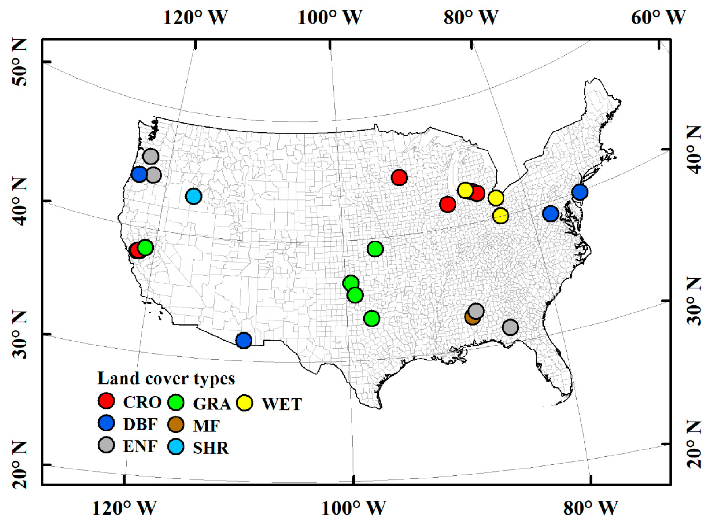
3.1. Study Domain

The conterminous United States (CONUS) encompasses a vast range of climates, landscapes and ecosystems and is chosen as the study domain to assess the performance of the PT-SinRH model. The study domain, the CONUS, is located between 70 and 130°W and 25 and 49°N (Figure 1). As the topography changes, the climate of the CONUS ranges from the humid subtropics of the southeast to the arid deserts of the southwest and the temperate forests of the Pacific Northwest to the polar climate of Alaska.

The CONUS has diverse land-cover types, including coniferous forests, broadleaf forests, grasslands, deserts and semi-arid areas, wetlands and montane vegetation. These ecosystems are distributed in different geographical and climatic regions, such as northern, western, eastern and central-western regions, which provide various effects on climate and ET. In addition, the CONUS boasts an extensive network, the AmeriFlux (https://ameriflux.lbl.gov, accessed on 1 May 2024), which offers high-quality observations of key variables relevant to ET estimation. We selected 28 flux stations evenly distributed in the study area. These flux tower sites cover seven major International Geosphere-Biosphere Programme (IGBP) land-cover types: cropland (CRO; seven sites), deciduous broadleaf forest (DBF; four sites), evergreen needleleaf forest (ENF; four sites), grass (GRA; six sites), mixed forest (MF; one site), shrubland (SHR; two sites), and wetland (WET; four sites). Details of these flux sites are shown in

Table 2. Information for the 28 EC flux tower sites over the CONUS, including the Identity (ID), site name, latitude (Lat), longitude (Lon), and International Geosphere-Biosphere Programme (IGBP) land-cover types.

ID	Site Name	Lat (N), Long (E)	IGBP	ID	Site Name	Lat (N), Long (E)	IGBP
1	US-AR1	36.4267, −99.4200	GRA	15	US-Snf	38.0402, −121.7272	GRA
2	US-Bi1	38.0992, −121.4993	CRO	16	US-Ton	38.4309, −120.9660	SHR
3	US-CMW	31.6637, −110.1777	DBF	17	US-Tw3	38.1152, −121.6469	CRO
4	US-IB1	41.8593, −88.2227	CRO	18	US-Var	38.4133, −120.9508	GRA
5	US-KL1	42.4847, −85.4422	CRO	19	US-Wpp	44.1369, −123.1824	DBF
6	US-KM1	42.4376, −85.3287	CRO	20	US-WPT	41.4646, −82.9962	WET
7	US-Me6	44.3233, −121.6078	ENF	21	US-xAB	45.7624, −122.3303	ENF
8	US-MWA	42.2143, −84.8539	CRO	22	US-xAE	35.4106, −99.0588	GRA
9	US-MWW	42.6689, −86.0229	WET	23	US-xBL	39.0603, −78.0716	DBF
10	US-Myb	38.0503, −121.7652	WET	24	US-xCL	33.4012, −97.5700	GRA
11	US-ORv	40.0201, −83.0183	WET	25	US-xDL	32.5417, −87.8039	MF
12	US-Ro6	44.6946, −93.0578	CRO	26	US-xJE	31.1948, −84.4686	ENF
13	US-Rws	43.1675, −116.7132	SHR	27	US-xKA	39.1104, −96.6129	GRA
14	US-Slt	39.9138, −74.5960	DBF	28	US-xTA	32.9505, −87.3933	ENF

.

3.2. Data

3.2.1. Eddy Covariance Measurements

We used the ET measurements from the ground-measured EC flux tower to validate the performance of the PT-SinRH model. The data were collected by 28 flux tower sites from AmeriFlux. The locations of these flux sites are evenly spread over diverse terrain across the CONUS, so the climate varies from snowy to dry. These datasets were combined with half-hourly or hourly ground-measured meteorological data, including T_a, T_max, RH, G, R_n and ET. To present a consistent temporal resolution of ET, the observation of daily ET was combined with half-hourly observations by using the approach developed by Reichstein et al. [29]. If the percentage of missing data in the daily data exceeded twenty-five percent, the data were considered missing. The energy closure imbalance [30] of the EC measurements was corrected using the Bowen ratio closure approach.

3.2.2. Satellite and Reanalysis Data

The satellite data we used were the NDVI and LAI products of the GLASS with a spatial resolution of 0.05° and a temporal resolution of 8 days. The GLASS products [31] employed the deep neural network (DNN) method from advanced very high-resolution radiometer (AVHRR) data (denoted as GLASS-AVHRR).

We also used T_a, T_max, RH, G and R_n from the MERRA2, which is generated by NASA’s Global Modelling and Assimilation Office (GMAO), utilizing atmospheric reanalysis from the satellite. This sophisticated atmospheric reanalysis dataset incorporates vast satellite data, encompassing novel observation categories like aerosols, microwaves, and hyperspectral radiation. To make better use of the data, we synthesized hourly data from MERRA2 into daily data, which were extracted from the pixels covering the EC sites with a spatial resolution of 1/2° × 2/3°.

4. Model Evaluation

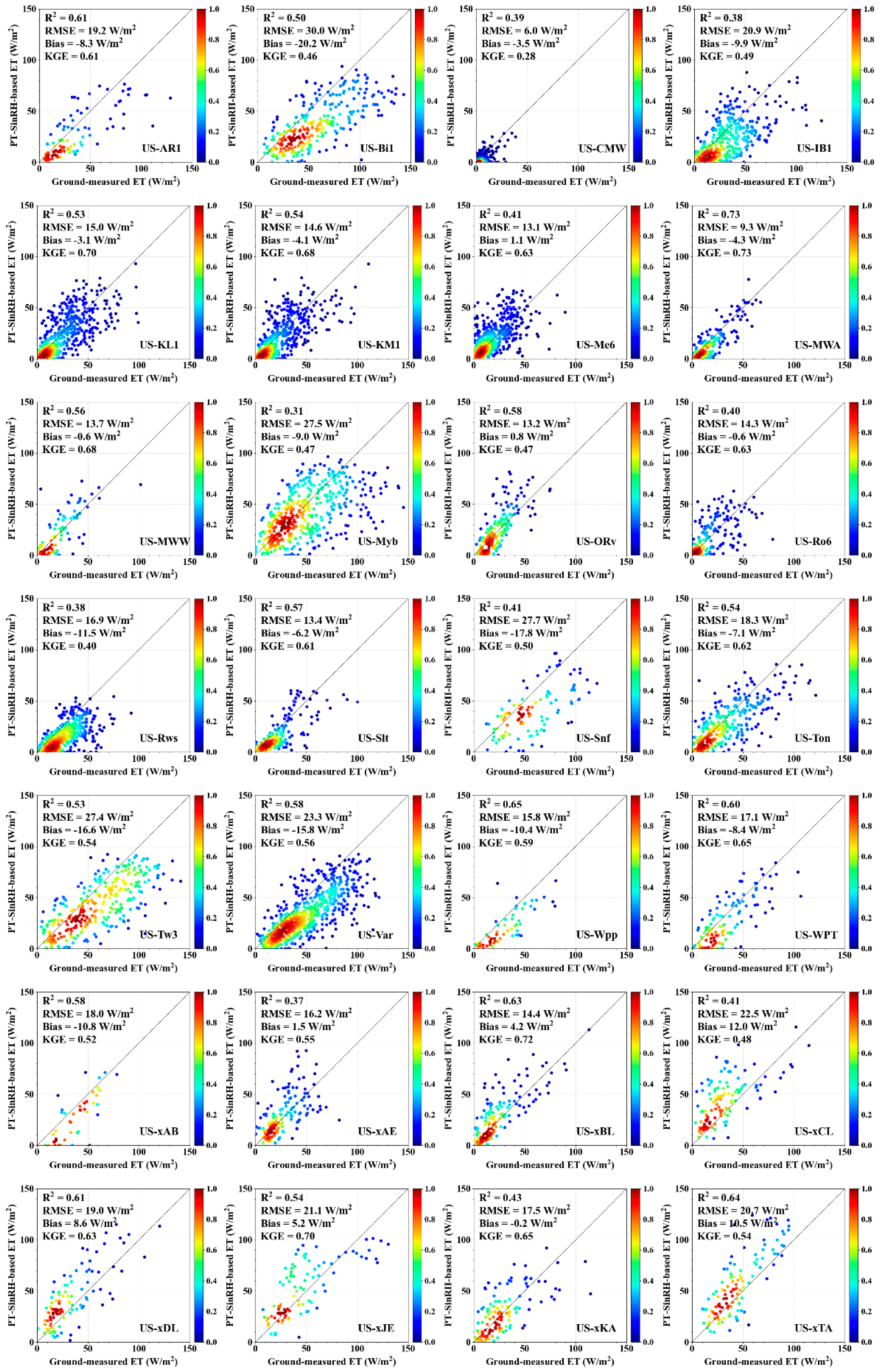
4.1. Model Validation Based on Site-Measured and Satellite Data Inputs

To assess the simulation performance of the PT-SinRH model, we conducted temporal validation as well as site validation. Compared with ET observations, estimated ET captures the variations of the observations on daily, seasonal, and annual scales (Figure 2). The validation results on the daily scale show that the PT-SinRH estimates fit the observations with an R² of 0.55, an RMSE of 17.5 W/m², a bias of −1.2 W/m² and a KGE of 0.70. The accuracy of seasonal estimates of PT-SinRH (R² = 0.71, RMSE = 13.3 W/m², bias = −4.5 W/m², KGE = 0.78) seems better than that of daily estimates. Our PT-SinRH model can capture the interannual variation, and the KGE and R² of the estimated annual anomalies are 0.43 and 0.44, and the RMSE and bias are 5.1 and 0.01 W/m², respectively. At the same time, PT-SinRH estimates fit the among-site variations. The KGE and R² of site average estimates are 0.71 and 0.61, and the RMSE and bias are 9.1 and −3.4 W/m², respectively.

To evaluate the PT-SinRH model, we validated the ET estimates against the observations at all 28 AmeriFlux sites (Figure 3). The R² and KGE range from 0.31 to 0.73 and from 0.40 to 0.73, respectively. The RMSE and bias range from 5.7 to 30.0 W/m², and from −20.2 to 12.0 W/m², respectively. Among all the sites, PT-SinRH performs best at the US-MWA site with an R² of 0.73, KGE of 0.73, RMSE of 9.3 W/m² and bias of −4.3 W/m². Simultaneously, the model has the lowest accuracy at the US-Rws site (R² = 0.38, RMSE = 16.9 W/m², bias = −11.5 W/m² and KGE = 0.40). The PT-SinRH model demonstrates different performances for various vegetation types. The model has an optimal performance in MF, with an average R² of 0.61, RMSE of 19.0 W/m², bias of 8.6 W/m² and KGE of 0.63, followed by DBF (average R² = 0.51, RMSE = 12.6 W/m², bias = −1.7 W/m² and KGE = 0.63). PT-SinRH performs worst in SHR, with as average R² of 0.46, RMSE of 17.6 W/m², bias of −9.3 W/m² and KGE of 0.51. The KGE descending order of all vegetation types is MF (0.63), DBF (0.63), ENF (0.62), CRO (0.60), WET (0.60), GRA (0.56) and SHR (0.51).

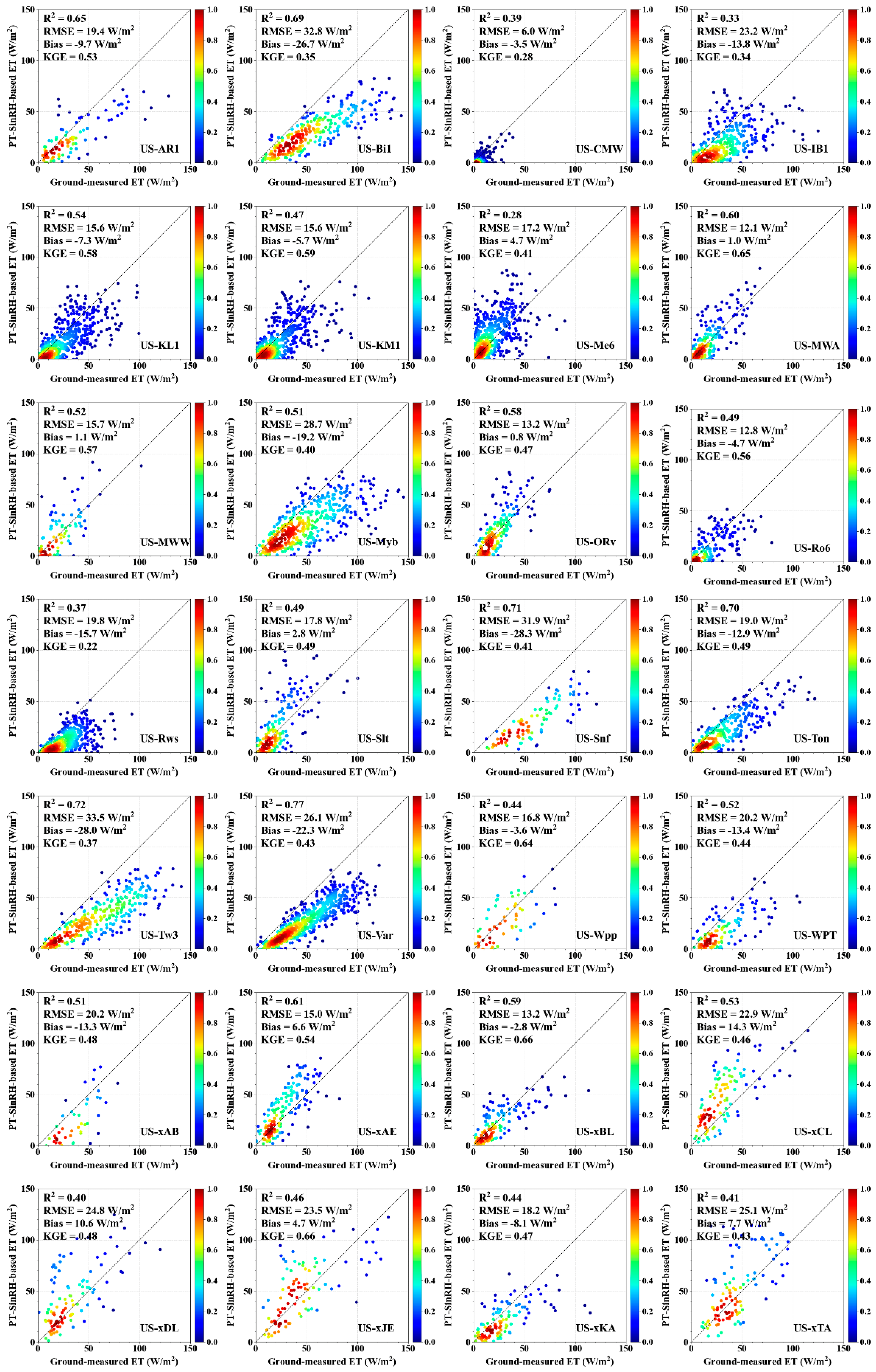
4.2. Model Validation Based on Reanalysis and Satellite Data Inputs

To evaluate the model based on reanalysis and satellite data inputs, we compared ground-measured and estimated ET across days, seasons, sites and years at all 28 sites (Figure 4). Figure 4 shows that the model has relatively accurate estimations for daily and seasonal ET. For daily ET estimates, the PT-SinRH model based on reanalysis and satellite data inputs has a KGE of 0.55, R² of 0.49, RMSE of 20.3 W/m² and bias of −8.6 W/m². The PT-SinRH based on reanalysis and satellite data inputs has the best performance in predicting seasonal variation ET, with the highest KGE value of 0.61, R² of 0.63 and RMSE and bias of 17.0 W/m² and −9.5 W/m², respectively. In forecasting the variability among sites, the PT-SinRH model exhibits a commendable performance. Its KGE is 0.54, and R², RMSE and bias values are 0.39, 13.4 W/m², and −7.5 W/m², respectively. Meanwhile, the PT-SinRH model can reproduce the interannual variation. Compared with the ground measurements, the KGE, R², RMSE and bias of the annual anomalies estimated by PT-SinRH are 0.36, 0.38, 5.0 W/m² and 0.01 W/m², correspondingly.

We contrast the corresponding ET estimates derived from PT-SinRH based on reanalysis and satellite data inputs with daily ET observations from all 28 sites (Figure 5). For the 28 sites, the estimated values range from 0.22 to 0.66 for the KGE of daily ground-measured ET, R² ranges from 0.28 to 0.77, RMSE ranges from 6.0 to 33.5 W/m² and bias ranges from −28.3 to 14.3 W/m². From the 28 sites, PT-SinRH based on reanalysis and satellite data inputs at the US-MWA site has excellent simulation accuracy, with a KGE performance of 0.65, R² of 0.6, RMSE of 12.1 W/m² and bias of 1.0 W/m². However, the estimation performance of ET of PT-SinRH at the US-Rws site is poor, with the lowest KGE of 0.22, R² of 0.37, RMSE of 19.8 W/m² and bias of −15.7 W/m². In addition, Figure 5 reflects the accuracy of the PT-SinRH model based on reanalysis and satellite data inputs for daily ET estimation under different land-cover types. The PT-SinRH model performs best in ENF, with an average KGE of 0.52, R² of 0.42, and RMSE of 20.3 W/m² and bias of −1.3 W/m². However, PT-SinRH performed the worst in CRO, with an average KGE of 0.33, R² of 0.55, RMSE of 20.8 W/m² and bias of −12.17 W/m². The KGE of the seven land-cover types was ranked in the following order: ENF (0.52) > DBF (0.51) > MF (0.48) > WET (0.47) = GRA (0.47) > SHR (0.36) > CRO (0.33).

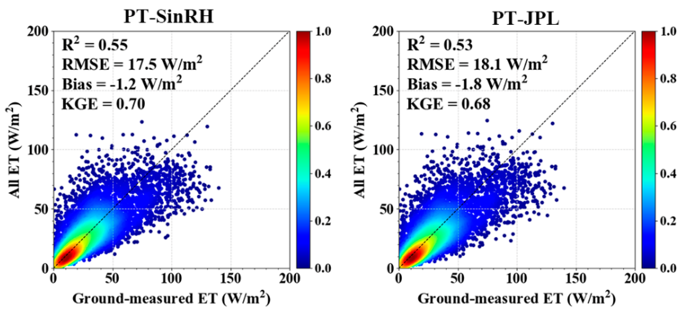
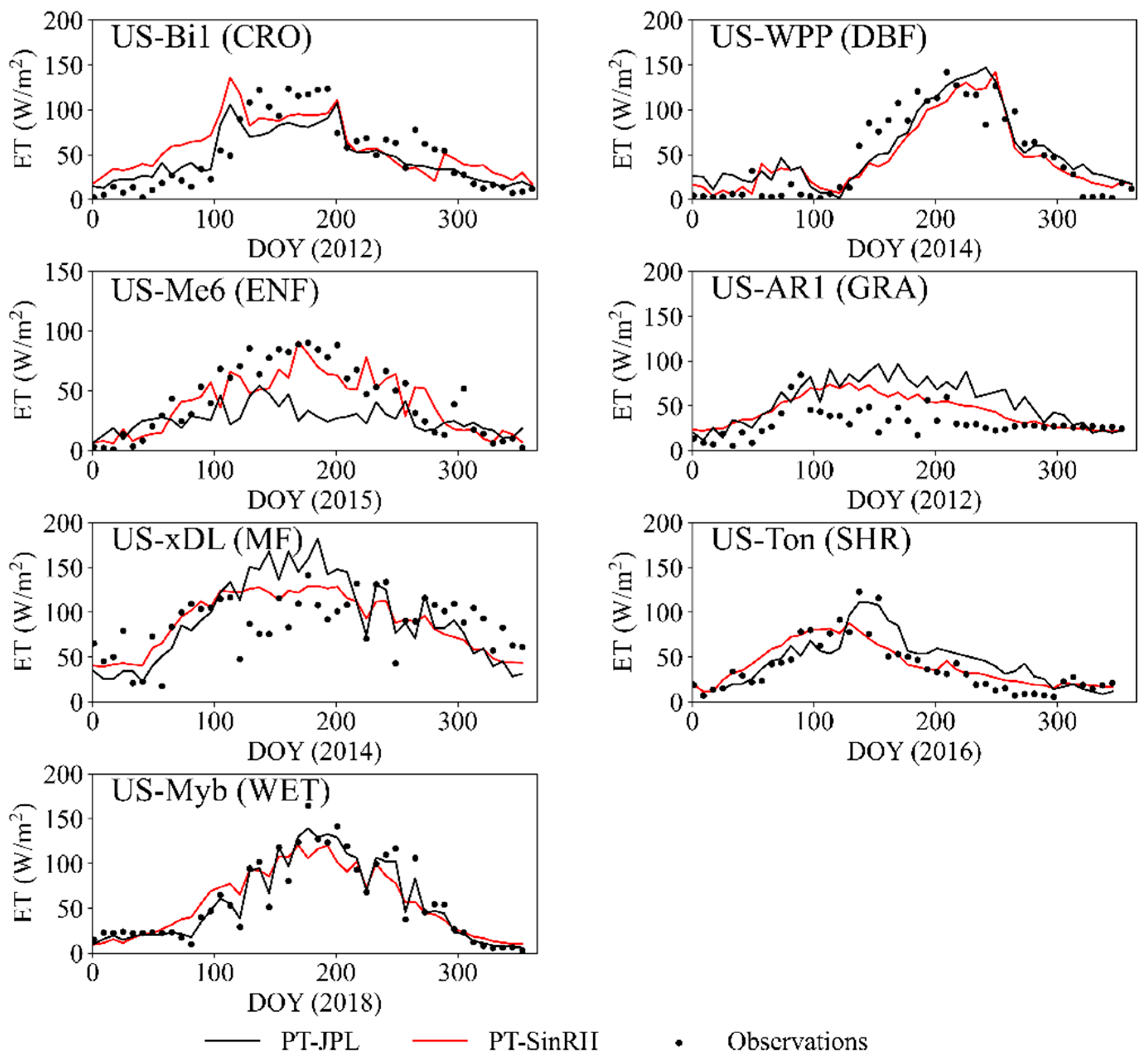
4.3. Comparison with the PT-JPL Model

We compared daily ET observations at all 28 sites and ET estimates for the different models driven by tower-specific data inputs (Figure 6). The results demonstrate that our approach improved ET estimates, increasing the KGE and R² by 0.02 and decreasing the RMSE by 0.6 W/m² (3.4%). Specifically, for daily ET estimates, the KGE of PT-SinRH is 0.70, whereas that of PT-JPL is 0.68. Furthermore, the R² for PT-SinRH is 0.55 (p < 0.01), with a corresponding bias of −1.2 W/m² and RMSE of 17.5 W/m². For PT-JPL, the R² is 0.53 (p < 0.01), accompanied by a bias of −1.8 W/m² and RMSE of 18.1 W/m². Notably, the results of PT-JPL have more outliers than the other.

The 8-day ET observations and estimates of PT-SinRH, as well as PT-JPL, for all vegetation types demonstrate similar seasonal variations during the year (Figure 7). However, they also have differences. Seasonal ET variations and magnitudes of both models are comparable. Both ET models have abilities to capture ET seasonal variations for all vegetation types.

Consistent with the preceding findings, PT-SinRH demonstrates enhanced efficacy in estimating daily ET driven by reanalysis and satellite data inputs (Figure 8). The outcome shows that our approach yields improved ET estimates, with an increase both in KGE and R² of 0.02, and a reduction in RMSE of 0.6 W/m² (2.9%). For daily ET estimation, the KGE of the PT-SinRH model is 0.55, slightly higher than the KGE of the PT-JPL model at 0.53. Furthermore, PT-SinRH exhibits an R² of 0.49 (p < 0.01), with a bias and RMSE of −8.6 W/m² and 20.3 W/m², respectively. In contrast, PT-JPL yields an R² of 0.47 (p < 0.01), with a bias and RMSE of −9.1 W/m² and 20.9 W/m², respectively. Overall, the improved model performs better than PT-JPL.

The 8-day ET time series example as ground-observed and estimated using PT-SinRH and PT-JPL models based on reanalysis and satellite data inputs showed similar and clear seasonal trends at seven sites with different land-cover types (Figure 9). However, despite the similar seasonal patterns, the specific values of ET for each land-cover type may vary throughout the year. Both the PT-SinRH and PT-JPL models are capable of capturing the seasonal changes of ET in the seven vegetation types.

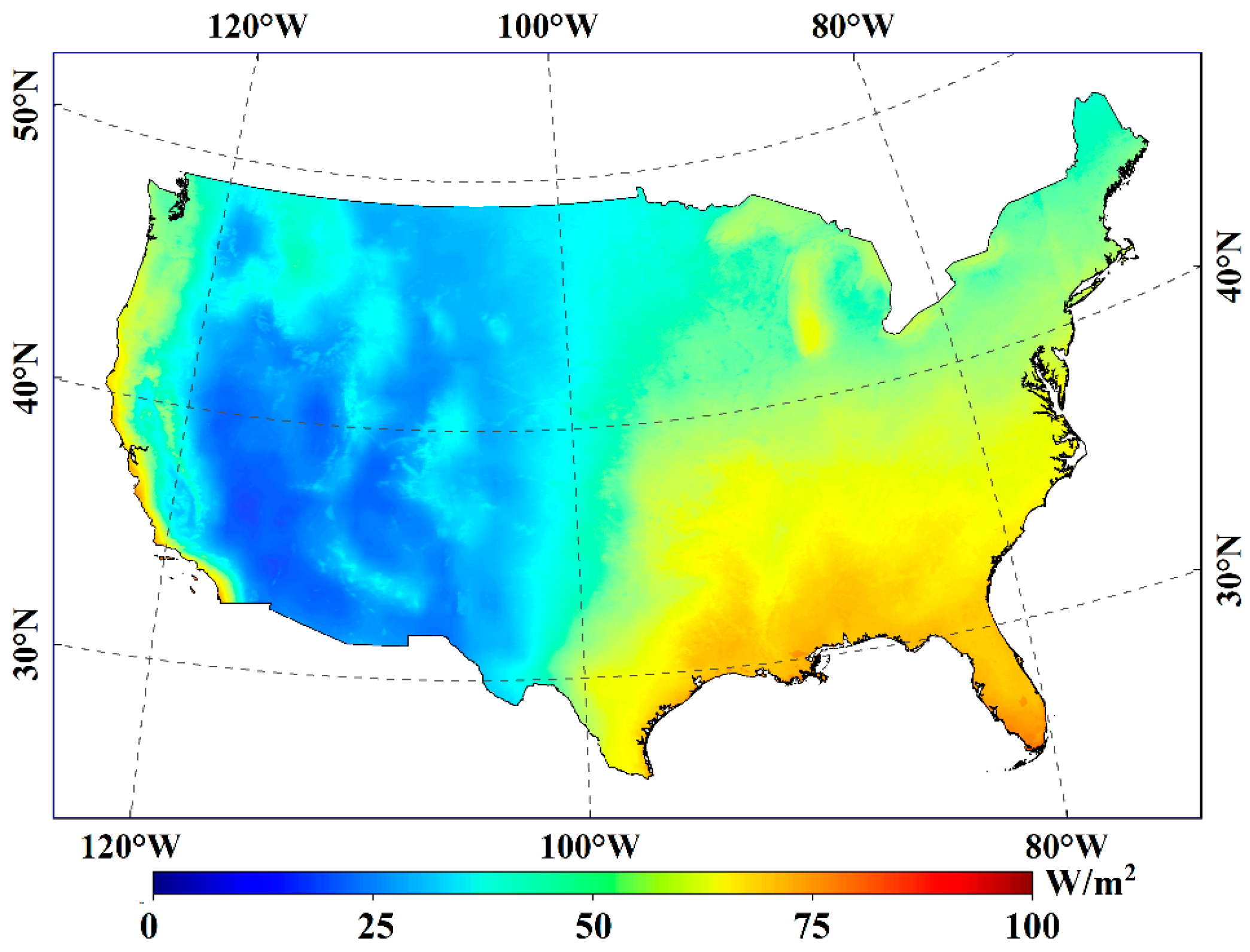
4.4. Mapping of PT-SinRH-Based Terrestrial ET Over CONUS

Figure 10 displays the spatial distribution of the average annual ET over a multiyear period (2003–2005). In the CONUS, the PT-SinRH model’s estimation of the annual mean ET from 2003 to 2005 is 41.81 W/m². Specifically, the region with lower ET is primarily found in the western United States, from 100°W to the west, where grasslands and shrublands make up the majority of the land-use type. Additionally, we discovered that the eastern CONUS, from 100°W eastward, was where the majority of the regions with higher ET were found. This region was also home to densely populated forests and croplands. More significantly, there was also a fair amount of precipitation in this area, which may have an impact on the moisture content of the surface soil and further regulate ET in this area.

5. Discussion

5.1. Model Performance

5.1.1. Ability of the PT-SinRH Model to Simulate ET

Based on the improved strategy of sinusoidal RH, the PT-SinRH model not only raised the accuracy of ET simulation but also yielded more robust estimates on the timescale, capturing especially well the seasonal variations of ET for all seven land-cover types. The model validation for all 28 sites showed that PT-SinRH could obtain higher R² and KGE and lower RMSE and bias, whether based on site-measured or reanalysis and satellite data inputs. Thus, PT-SinRH provided a better modeled system than the original PT-JPL model in the simulation of ET.

The PT-SinRH model has different abilities to simulate ET for sites with different land-cover types. ET estimations are more accurate at ENF and DBF sites, with the bias values between −10.8 W/m² and 5.2 W/m² based on site-measured inputs, and the seasonal variances of ET were also captured well, with consistent curves with ground measurements, which might result from less water stress of the energy-driven ET for high-latitude coniferous forests due to slower vegetation transpiration [32]. However, the performance of the PT-SinRH model trends to be worse for CRO sites (e.g., US-Bi1, US-IB1 and US-KM1) with a negative bias and lower R², which can be explained by the actual high ET resulting from agricultural activities such as irrigation [33]. On the other hand, the underestimation at GRA sites is probably attributable to the fact that the high SM and low vegetation cover on the grassland lead to reduced vegetation transpiration but also enhanced soil evaporation [34].

The soil moisture constraint is one of the variables that contributed most to the uncertainty of the PT-JPL model in ET estimations [35]. According the hypothesis of Bouchet [36], SM can be reflected by atmospheric humidity near the surface. The introduction of VPD in the equation is meant to quantify the evaporation response, and the relative sensitivity of SM to VPD is defined by the β parameter [17]. However, the acquisition of VPD data, whether through the measurements derived from flux towers or retrieval derived from remote sensing products, presents a large error [37]. Additionally, the relationship between SM, RH and soil evaporation follows a distinctive pattern. Initially, soil evaporation increases rapidly with the rise in SM and RH. This is followed by a phase where the increase in soil evaporation becomes linear with the continued rise in SM and relative humidity [17]. Eventually, the increase in soil evaporation slows down, becoming more gradual as SM and RH continue to rise. Consequently, the relationship between soil evaporation and the changes in SM and RH can be described by an S-shaped function. We have successfully captured the relationship between soil evaporation and RH using Equation 3, which enables us to accurately estimate soil evaporation. Undoubtedly, the PT-SinRH model has improved the accuracy of ET estimations compared with the original PT-JPL model.

In addition, due to the mismatch of spatial scales, the model based on site measurements can estimate ET more reliably than those based on reanalysis data [38]. Comparing the evaluation metrics in Figure 8, the PT-JPL and PT-SinRH validated by daily ET observations for all 28 sites in Figure 6 yield a better performance, with KGR increased by 0.15 and RMSE decreased by 2.8 W/m². Further comparison of model performance based on different inputs at each site revealed a consistent result, with the largest KGE increase (0.22) at the US-Me6 site and the largest decrease in RMSE (6.1 W/m²) at the US-Tw3 site.

5.1.2. Uncertainty in the PT-SinRH Estimates

PT-SinRH still has considerable uncertainty in the estimation of ET, although the parameters of the model have been improved. These uncertainties are mainly caused by three aspects: data sources, scaling effects and model structure.

The uncertainties caused by data sources are attributed to EC measurements derived from in situ sites and meteorological variables derived from reanalysis data. EC measurements suffer from various errors and an ambiguous interpretation of flux values, although they are relatively accurate in general [39]. When it comes to energy imbalance, the measurement errors of the energy balance equation’s component parts typically range from 5% to 20% [30]. The method of Bowen ratio correcting EC flux [40] was applied in the study to achieve energy balance closure, but there still remains at least a 10% error in measured ET [41]. Furthermore, the absence of ground-measured data also affects the stability of the model and accuracy of time series analysis. At the 28 AmeriFlux tower sites, these otherwise available measurements were lost due to the interference of anomalies in sensor status or weather conditions. In addition, a large deviation of meteorological reanalysis data from in situ measurements and the inaccurate estimation of surface energy budgets also make the PT-SinRH model inherit more uncertainty through the input of datasets [42,43,44].

Scaling effects are the second problem introducing uncertainty, caused by the mismatched spatial scale between the in situ sites and the grid of reanalysis and satellite data [45]. The size and shape of the footprint of flux towers is generally only a few hundred meters, depending on different facilities and environmental conditions [46]. Due to the limited spatial representation of in situ measurements, it is difficult to accurately evaluate EC estimates at the pixel scale of remote sensing products, especially over heterogeneous landscapes and vegetation covers [13]. The scaling effects can produce relative errors of 5–25% in model validation based on EC measurements [47].

PT-JPL is considered as a simplified version of the Penman equation [17]. We improved the characterization of soil water constraints in PT-SinRH, but the new model retained certain limitations in ET estimations. In fact, the PT-SinRH model keeps constant parameters for all land-cover types, although some are space-varying, which could reduce the reliability of the model over complex underlying surfaces [48]. Meanwhile, the PT-SinRH model does not consider aerodynamic and surface resistance, which avoids the propagation of uncertainties but may be error prone in areas with strong winds and low surface roughness [49]. In terms of canopy transpiration, the uncertainty of vegetation characteristics (e.g., height and density) is also not considered, resulting in more errors in ET estimations [50].

5.2. Merits and Limitations of the PT-SinRH Model

The PT-SinRH model has two advantages compared to PT-JPL. Firstly, PT-SinRH is based on RH rather than VPD to characterize soil moisture constraints, which can improve the estimation accuracy of ET because RH is easier to obtain and more accurate than VPD. A strong correlation between VPD and near-surface air temperature has been confirmed [51,52]. Near-surface air temperature and RH are two key parameters for calculating VPD, and their accuracy will determine the estimation accuracy of VPD [37]. At the same time, the model characterizes the nonlinear effect of RH on ET by introducing a sine function, which further improves the accuracy of remote sensing models. Therefore, the model has higher reliability and robustness. Secondly, the model greatly enhances the feasibility of estimating ET because PT-SinRH introduces RH to characterize soil moisture constraints, which requires only RH rather than SM data. At present, reliable SM datasets in many models are unavailable [53]. Therefore, the model only needs four input variables: T_a, R_n, RH and NDVI, which is highly operable and can be widely used in ET estimation.

Nonetheless, the PT-SinRH model also has distinct limitations. Firstly, although the new model has a strong performance, PT-SinRH uses RH to reflect SM constraints, while the actual SM is not considered in our model. Purdy et al. [28] showed that RMSE and bias could be reduced by 22.7% and 29.9%, respectively, when SM was considered in soil evaporation. Therefore, the model has certain limitations in estimating the contribution of accurate soil evaporation to ET. Secondly, the PT-SinRH model does not consider the changes in the Priestley–Taylor coefficient α during the vegetation growth season on the underlying surface. Several studies have shown that the Priestley–Taylor coefficient α varies both diurnally and seasonally [54] and is related to the underlying surface and vegetation growth [55]. Therefore, there may be certain limitations in the application of the model, and the determination of α is particularly important. Thirdly, the influence of aerodynamic roughness length on ET is not considered in PT-SinRH. Several studies have shown that aerodynamic roughness length is very sensitive to remote sensing calculation of ET, and its accuracy directly affects the accuracy of surface flux calculation [56,57,58]. Therefore, the model still has certain limitations.

6. Conclusions

The purpose of this study was to improve the PT-JPL method to obtain more accurate ET estimates. The method (PT-SinRH) was developed by making use of RH instead of VPD in the calculation of soil moisture constraints. We collected 28 EC sites from 2000 to 2020 to validate PT-SinRH by using site and MERRA2 meteorological data as input. Additionally, we compared PT-SinRH with the PT-JPL model. The main conclusions in the study are as follows:

(1) The validation results showed that PT-SinRH ET estimates have a suitable accuracy based on ground-measurements across days, seasons, sites and years at all 28 sites.

(2) The validation results of PT-SinRH that were based on site-measured and satellite data inputs outperformed those which were based on reanalysis and satellite data inputs.

(3) The PT-SinRH method outperformed the PT-JPL method, both based on reanalysis and combing site-measured satellite data inputs, and both methods could capture the trend variation in different land-cover types.

References

1. Wang, K.; Dickinson, R.E. A review of global terrestrial evapotranspiration: Observation, modeling, climatology, and climatic variability. Rev. Geophys. 2012, 50. [Google Scholar] [CrossRef]
2. Allen, R.G.; Pereira, L.S.; Howell, T.A.; Jensen, M.E. Evapotranspiration information reporting: I. Factors governing measurement accuracy. Agric. Water Manag. 2011, 98, 899–920. [Google Scholar] [CrossRef]
3. Mu, Q.; Heinsch, F.A.; Zhao, M.; Running, S.W. Development of a global evapotranspiration algorithm based on MODIS and global meteorology data. Remote Sens. Environ. 2007, 111, 519–536. [Google Scholar] [CrossRef]
4. Liang, S.L.; Wang, K.C.; Zhang, X.T.; Wild, M. Review on estimation of land surface radiation and energy budgets from ground measurement, remote sensing and model simulations. IEEE J. Sel. Top. Appl. Earth Obs. Remote Sens. 2010, 3, 225–240. [Google Scholar] [CrossRef]
5. Xu, Z.W.; Liu, S.M.; Zhu, Z.L.; Zhou, J.; Shi, W.J.; Xu, T.R.; Yang, X.F.; Zhang, Y.; He, X.L. Exploring evapotranspiration changes in a typical endorheic basin through the integrated observatory network. Agric. For. Meteorol. 2020, 290, 108010. [Google Scholar] [CrossRef]
6. Fisher, J.B.; Melton, F.; Middleton, E.; Hain, C.; Anderson, M.; Allen, R.; McCabe, M.F.; Hook, S.; Baldocchi, D.; Townsend, P.A.; et al. The future of evapotranspiration: Global requirements for ecosystem functioning, carbon and climate feedbacks, agricultural management, and water resources. Water Resour. Res. 2017, 53, 2618–2626. [Google Scholar] [CrossRef]
7. Yao, Y.J.; Liang, S.L.; Li, X.L.; Chen, J.Q.; Wang, K.C.; Jia, K.; Cheng, J.; Jiang, B.; Fisher, J.B.; Mu, Q.Z.; et al. A satellite-based hybrid algorithm to determine the Priestley-Taylor parameter for global terrestrial latent heat flux estimation across multiple biomes. Remote Sens. Environ. 2015, 165, 216. [Google Scholar] [CrossRef]
8. Condon, L.E.; Atchley, A.L.; Maxwell, R.M. Evapotranspiration depletes groundwater under warming over the contiguous United States. Nat. Commun. 2020, 11, 873. [Google Scholar] [CrossRef] [PubMed]
9. Fisher, J.B.; Lee, B.; Purdy, A.J.; Halverson, G.H.; Dohlen, M.B.; Cawse-Nicholson, K.; Wang, A.; Anderson, R.G.; Aragon, B.; Arain, M.A.; et al. ECOSTRESS: NASA’s next generation mission to measure evapotranspiration from the International Space Station. Water Resour. Res. 2020, 56, e2019WR026058. [Google Scholar] [CrossRef]
10. Brust, C.; Kimball, J.S.; Maneta, M.P.; Jencso, K.; He, M.Z.; Reichle, R.H. Using SMAP Level-4 soil moisture to constrain MOD16 evapotranspiration over the contiguous USA. Remote Sens. Environ. 2021, 255, 112277. [Google Scholar] [CrossRef]
11. Su, Z. The Surface Energy Balance System (SEBS) for estimation of turbulent heat fluxes. Hydrol. Earth Syst. Sci. 2002, 6, 85–99. [Google Scholar] [CrossRef]
12. Yao, Y.J.; Liang, S.L.; Yu, J.; Chen, J.Q.; Liu, S.M.; Lin, Y.; Fisher, J.B.; McVicar, T.R.; Cheng, J.; Jia, K.; et al. A simple temperature domain two-source model for estimating agricultural field surface energy fluxes from Landsat images. J. Geophys. Res.-Atmos. 2017, 122, 5211–5236. [Google Scholar] [CrossRef]
13. Kalma, J.D.; McVicar, T.R.; McCabe, M.F. Estimating Land Surface Evaporation: A Review of Methods Using Remotely Sensed Surface Temperature Data. Surv. Geophys. 2008, 29, 421–469. [Google Scholar] [CrossRef]
14. Mu, Q.Z.; Zhao, M.S.; Running, S.W. Improvements to a MODIS global terrestrial evapotranspiration algorithm. Remote Sens. Environ. 2011, 115, 1781–1800. [Google Scholar] [CrossRef]
15. Shuttleworth, W.J.; Wallace, J.S. Evaporation from Sparse Crops—An Energy Combination Theory. Q. J. R. Meteor. Soc. 1985, 111, 839–855. [Google Scholar] [CrossRef]
16. Monteith, J.I.L. Evaporation and Environment. Symp. Soc. Exp. Biol. 1965, 19, 205–234. [Google Scholar]
17. Fisher, J.B.; Tu, K.P.; Baldocchi, D.D. Global estimates of the land–atmosphere water flux based on monthly AVHRR and ISLSCP-II data, validated at 16 FLUXNET sites. Remote Sens. Environ. 2008, 112, 901–919. [Google Scholar] [CrossRef]
18. Priestley, C.H.B.; Taylor, R.J. On the Assessment of Surface Heat Flux and Evaporation Using Large Scale Parameters. Mon. Weather Rev. 1972, 100, 81–92. [Google Scholar] [CrossRef]
19. Jung, M.; Koirala, S.; Weber, U.; Ichii, K.; Gans, F.; Camps-Valls, G.; Papale, D.; Schwalm, C.; Tramontana, G.; Reichstein, M. The FLUXCOM ensemble of global land-atmosphere energy fluxes. Sci. Data 2019, 6, 74. [Google Scholar] [CrossRef]
20. Li, X.; Liu, S.M.; Li, H.X.; Ma, Y.F.; Wang, J.H.; Zhang, Y.; Xu, Z.W.; Xu, T.R.; Song, L.S.; Yang, X.F.; et al. Intercomparison of Six Upscaling Evapotranspiration Methods: From Site to the Satellite Pixel. J. Geophys. Res.-Atmos. 2018, 123, 6777–6803. [Google Scholar] [CrossRef]
21. Bateni, S.M.; Entekhabi, D.; Jeng, D.S. Variational assimilation of land surface temperature and the estimation of surface energy balance components. J. Hydrol. 2013, 481, 143–156. [Google Scholar] [CrossRef]
22. Pipunic, R.C.; Walker, J.P.; Western, A. Assimilation of remotely sensed data for improved latent and sensible heat flux prediction: A comparative synthetic study. Remote Sens. Environ. 2008, 112, 1295–1305. [Google Scholar] [CrossRef]
23. Mao, J.F.; Fu, W.T.; Shi, X.Y.; Ricciuto, D.M.; Fisher, J.B.; Dickinson, R.E.; Wei, Y.X.; Shem, W.; Piao, S.L.; Wang, K.C.; et al. Disentangling climatic and anthropogenic controls on global terrestrial evapotranspiration trends. Environ. Res. Lett. 2015, 10, 094008. [Google Scholar] [CrossRef]
24. Talsma, C.J.; Good, S.P.; Jimenez, C.; Martens, B.; Fisher, J.B.; Miralles, D.G.; McCabe, M.F.; Purdy, A.J. Partitioning of evapotranspiration in remote sensing-based models. Agric. For. Meteorol. 2018, 260, 131–143. [Google Scholar] [CrossRef]
25. Ershadi, A.; McCabe, M.F.; Evans, J.P.; Chaney, N.W.; Wood, E.F. Multi-site evaluation of terrestrial evaporation models using FLUXNET data. Agric. For. Meteorol. 2014, 187, 46–61. [Google Scholar] [CrossRef]
26. Anderson, M.C.; Yang, Y.; Xue, J.; Knipper, K.R.; Yang, Y.; Gao, F.; Hain, C.R.; Kustas, W.P.; Cawse-Nicholson, K.; Hulley, G.; et al. Interoperability of ECOSTRESS and Landsat for mapping evapotranspiration time series at sub-field scales. Remote Sens. Environ. 2021, 252, 112189. [Google Scholar] [CrossRef]
27. Vinukollu, R.K.; Wood, E.F.; Ferguson, C.R.; Fisher, J.B. Global estimates of evapotranspiration for climate studies using multi-sensor remote sensing data: Evaluation of three process-based approaches. Remote Sens. Environ. 2011, 115, 801–823. [Google Scholar] [CrossRef]
28. Purdy, A.J.; Fisher, J.B.; Goulden, M.L.; Colliander, A.; Halverson, G.; Tu, K.; Farniglietti, J.S. SMAP soil moisture improves global evapotranspiration. Remote Sens. Environ. 2018, 219, 1–14. [Google Scholar] [CrossRef]
29. Reichstein, M.; Falge, E.; Baldocchi, D.; Papale, D.; Aubinet, M.; Berbigier, P.; Bernhofer, C.; Buchmann, N.; Gilmanov, T.; Granier, A.; et al. On the separation of net ecosystem exchange into assimilation and ecosystem respiration: Review and improved algorithm. Glob. Chang. Biol. 2005, 11, 1424–1439. [Google Scholar] [CrossRef]
30. Foken, T. The energy balance closure problem: An overview. Ecol. Appl. 2008, 18, 1351–1367. [Google Scholar] [CrossRef]
31. Xie, Z.J.; Yao, Y.J.; Zhang, X.T.; Liang, S.L.; Fisher, J.B.; Chen, J.Q.; Jia, K.; Shang, K.; Yang, J.M.; Yu, R.Y.; et al. The Global LAnd Surface Satellite (GLASS) evapotranspiration product Version 5.0: Algorithm development and preliminary validation. J. Hydrol. 2022, 610, 127990. [Google Scholar] [CrossRef]
32. Yao, Y.; Zhang, Y.; Zhao, S.; Li, X.; Jia, K. Evaluation of three satellite-based latent heat flux algorithms over forest ecosystems using eddy covariance data. Environ. Monit. Assess. 2015, 187, 382. [Google Scholar] [CrossRef] [PubMed]
33. Bai, P. Comparison of remote sensing evapotranspiration models: Consistency, merits, and pitfalls. J. Hydrol. 2023, 617, 128856. [Google Scholar] [CrossRef]
34. Yao, Y.; Liang, S.; Cheng, J.; Liu, S.; Fisher, J.B.; Zhang, X.; Jia, K.; Zhao, X.; Qin, Q.; Zhao, B. MODIS-driven estimation of terrestrial latent heat flux in China based on a modified Priestley–Taylor algorithm. Agric. For. Meteorol. 2013, 171, 187–202. [Google Scholar] [CrossRef]
35. García, M.; Sandholt, I.; Ceccato, P.; Ridler, M.; Mougin, E.; Kergoat, L.; Morillas, L.; Timouk, F.; Fensholt, R.; Domingo, F. Actual evapotranspiration in drylands derived from in-situ and satellite data: Assessing biophysical constraints. Remote Sens. Environ. 2013, 131, 103–118. [Google Scholar] [CrossRef]
36. Bouchet, R. Evapotranspiration reelle at potentielle, signification climatique. Int. Assoc. Sci. Hydro. Pub. 1963, 62, 134–142. [Google Scholar]
37. Zhang, H.; Wu, B.; Yan, N. Remote sensing estimates of vapor pressure deficit: An overview. Adv. Earth Sci. 2014, 29, 559. [Google Scholar]
38. Zhang, L.; Marshall, M.; Nelson, A.; Vrieling, A. A global assessment of PT-JPL soil evaporation in agroecosystems with optical, thermal, and microwave satellite data. Agric. For. Meteorol. 2021, 306, 108455. [Google Scholar] [CrossRef]
39. Mahrt, L. Computing turbulent fluxes near the surface: Needed improvements. Agric. For. Meteorol. 2010, 150, 501–509. [Google Scholar] [CrossRef]
40. Twine, T.E.; Kustas, W.; Norman, J.; Cook, D.; Houser, P.; Meyers, T.; Prueger, J.; Starks, P.; Wesely, M. Correcting eddy-covariance flux underestimates over a grassland. Agric. For. Meteorol. 2000, 103, 279–300. [Google Scholar] [CrossRef]
41. Finnigan, J.J.; Clement, R.; Malhi, Y.; Leuning, R.; Cleugh, H. A re-evaluation of long-term flux measurement techniques part I: Averaging and coordinate rotation. Bound.-Layer Meteorol. 2003, 107, 1–48. [Google Scholar] [CrossRef]
42. Badgley, G.; Fisher, J.B.; Jiménez, C.; Tu, K.P.; Vinukollu, R. On uncertainty in global terrestrial evapotranspiration estimates from choice of input forcing datasets. J. Hydrometeorol. 2015, 16, 1449–1455. [Google Scholar] [CrossRef]
43. Rienecker, M.M.; Suarez, M.J.; Gelaro, R.; Todling, R.; Bacmeister, J.; Liu, E.; Bosilovich, M.G.; Schubert, S.D.; Takacs, L.; Kim, G.-K. MERRA: NASA’s modern-era retrospective analysis for research and applications. J. Clim. 2011, 24, 3624–3648. [Google Scholar] [CrossRef]
44. Zhao, M.; Running, S.W.; Nemani, R.R. Sensitivity of Moderate Resolution Imaging Spectroradiometer (MODIS) terrestrial primary production to the accuracy of meteorological reanalyses. J. Geophys. Res. Biogeosci. 2006, 111. [Google Scholar] [CrossRef]
45. Yao, Y.; Liang, S.; Li, X.; Zhang, Y.; Chen, J.; Jia, K.; Zhang, X.; Fisher, J.B.; Wang, X.; Zhang, L. Estimation of high-resolution terrestrial evapotranspiration from Landsat data using a simple Taylor skill fusion method. J. Hydrol. 2017, 553, 508–526. [Google Scholar] [CrossRef]
46. Turner, D.P.; Ritts, W.D.; Cohen, W.B.; Gower, S.T.; Zhao, M.; Running, S.W.; Wofsy, S.C.; Urbanski, S.; Dunn, A.L.; Munger, J. Scaling gross primary production (GPP) over boreal and deciduous forest landscapes in support of MODIS GPP product validation. Remote Sens. Environ. 2003, 88, 256–270. [Google Scholar] [CrossRef]
47. Li, Z.-L.; Tang, R.; Wan, Z.; Bi, Y.; Zhou, C.; Tang, B.; Yan, G.; Zhang, X. A review of current methodologies for regional evapotranspiration estimation from remotely sensed data. Sensors 2009, 9, 3801–3853. [Google Scholar] [CrossRef]
48. Bai, P.; Cai, C. Applicability evaluation of soil moisture constraint algorithms in remote sensing evapotranspiration models. J. Hydrol. 2023, 623, 129870. [Google Scholar] [CrossRef]
49. Marshall, M.; Tu, K.; Andreo, V. On parameterizing soil evaporation in a direct remote sensing model of ET: PT-JPL. Water Resour. Res. 2020, 56, e2019WR026290. [Google Scholar] [CrossRef]
50. Schenk, H.J.; Jackson, R.B. Rooting depths, lateral root spreads and below-ground/above-ground allometries of plants in water-limited ecosystems. J. Ecol. 2002, 90, 480–494. [Google Scholar] [CrossRef]
51. Benali, A.; Carvalho, A.C.; Nunes, J.P.; Carvalhais, N.; Santos, A. Estimating air surface temperature in Portugal using MODIS LST data. Remote Sens. Environ. 2012, 124, 108–121. [Google Scholar] [CrossRef]
52. Hashimoto, H.; Dungan, J.L.; White, M.A.; Yang, F.; Michaelis, A.R.; Running, S.W.; Nemani, R.R. Satellite-based estimation of surface vapor pressure deficits using MODIS land surface temperature data. Remote Sens. Environ. 2008, 112, 142–155. [Google Scholar] [CrossRef]
53. Mallick, K.; Bhattacharya, B.K.; Patel, N.K. Estimating volumetric surface moisture content for cropped soils using a soil wetness index based on surface temperature and NDVI. Agric. For. Meteorol. 2009, 149, 1327–1342. [Google Scholar] [CrossRef]
54. McNaughton, K.; Spriggs, T.W. An evaluation of the Priestley and Taylor equation and the complementary relationship using results from a mixed-layer model of the convective boundary layer. Estim. Areal Evapotranspiration 1989, 177, 89–104. [Google Scholar]
55. Brutsaert, W. A generalized complementary principle with physical constraints for land-surface evaporation. Water Resour. Res. 2015, 51, 8087–8093. [Google Scholar] [CrossRef]
56. Kustas, W.P.; Moran, M.S.; Humes, K.S.; Stannard, D.I.; Pinter, P.J.; Hipps, L.E.; Swiatek, E.; Goodrich, D.C. Surface-Energy Balance Estimates at Local and Regional Scales Using Optical Remote-Sensing from an Aircraft Platform and Atmospheric Data Collected over Semiarid Rangelands. Water Resour. Res. 1994, 30, 1241–1259. [Google Scholar] [CrossRef]
57. Pitman, A.J. Assessing the Sensitivity of a Land-Surface Scheme to the Parameter Values Using a Single-Column Model. J. Clim. 1994, 7, 1856–1869. [Google Scholar] [CrossRef]
58. Zhou, Y.L.; Sun, X.M.; Zhu, Z.L.; Zhang, R.H.; Tian, J.; Liu, Y.F.; Guan, D.X.; Yuan, G.F. Surface roughness length dynamic over several different surfaces and its effects on modeling fluxes. Sci. China Ser. D 2006, 49, 262–272. [Google Scholar] [CrossRef]
Figure 1. Locations of the 28 sites used in this study.
Remotesensing 16 02783 g001
Figure 2. The estimated ET (vertical axis) versus the ground-measured ET (horizontal axis) based on site-measured and satellite data inputs for all ET, seasonal ET, among-site ET variability and annual ET anomalies.
Remotesensing 16 02783 g002
Figure 3. Comparison of the daily ET observations for all 28 sites and the corresponding ET estimations from PT-SinRH based on site-measured and satellite data inputs.
Remotesensing 16 02783 g003
Figure 4. The estimated ET (vertical axis) versus the ground-measured ET (horizontal axis) based on reanalysis and satellite data inputs for all ET, seasonal ET, among-site ET variability and annual ET anomalies.
Remotesensing 16 02783 g004
Figure 5. Comparison of the daily ET observations for all 28 sites and the corresponding ET estimations from PT-SinRH based on reanalysis and satellite data inputs.
Remotesensing 16 02783 g005
Figure 6. Comparison of the daily ET observations for all 28 sites and the corresponding ET estimations from PT-sinRH (left) and PT-JPL (right) based on site-measured and satellite data inputs.
Remotesensing 16 02783 g006
Figure 7. Time series example of 8-day ET as ground-measured and estimated using PT-sinRH and PT-JPL models based on site-measured and satellite data inputs at seven validation sites.
Remotesensing 16 02783 g007
Figure 8. Comparison of the daily ET observations for all 28 sites and the corresponding ET estimations from PT-sinRH (left) and PT-JPL (right) based on reanalysis and satellite data inputs.
Remotesensing 16 02783 g008
Figure 9. Eight-day ET time series example as ground-observed and estimated using PT-SinRH and PT-JPL models based on reanalysis and satellite data inputs.
Remotesensing 16 02783 g009
Figure 10. Maps of the annual CONUS ET averaged for 2003–2005 using the PT-SinRH model.
Remotesensing 16 02783 g010