Parcel-Based Sugarcane Mapping Using Smoothed Sentinel-1 Time Series Data

Abstract

The timely and accurate mapping of sugarcane cultivation is significant to ensure the sustainability of the sugarcane industry, including sugarcane production, rural society, sugar futures, and crop insurance. Synthetic aperture radar (SAR), due to its all-weather and all-time imaging capability, plays an important role in mapping sugarcane cultivation in cloudy areas. However, the inherent speckle noise of SAR data worsens the “salt and pepper” effect in the sugarcane map. Therefore, in previous studies, an additional land cover map or optical image was still required. This study proposes a new application paradigm of time series SAR data for sugarcane mapping to tackle this limitation. First, the locally estimated scatterplot smoothing (LOESS) smoothing technique was exploited to reconstruct time series SAR data and reduce SAR noise in the time domain. Second, temporal importance was evaluated using RF MDA ranking, and basic parcel units were obtained only based on multi-temporal SAR images with high importance values. Lastly, the parcel-based classification method, combining time series smoothing SAR data, RF classifier, and basic parcel units, was used to generate a sugarcane extent map without unreasonable sugarcane spots. The proposed paradigm was applied to map sugarcane cultivation in Suixi County, China. Results showed that the proposed paradigm was able to produce an accurate sugarcane cultivation map with an overall accuracy of 96.09% and a Kappa coefficient of 0.91. Compared with the pixel-based classification result with original time series SAR data, the new paradigm performed much better in reducing the “salt and pepper” spots and improving the completeness of the sugarcane plots. In particular, the unreasonable non-vegetation spots in the sugarcane map were eliminated. The results demonstrated the efficacy of the new paradigm for mapping sugarcane cultivation. Unlike traditional methods that rely on optical remote sensing data, the new paradigm offers a high level of practicality for mapping sugarcane in large regions. This is particularly beneficial in cloudy areas where optical remote sensing data is frequently unavailable.

1. Introduction

Sugarcane (Saccharum spp.) is a species of tall perennial grass. It is the major raw material source of manufactured sugar and is also used as a bioenergy feedstock for ethanol production [1,2,3,4]. Due to the increasing demand for sugar consumption and the economic impact on sustainable energy production, global sugarcane cultivation has increased significantly from 1994 to 2018 [5,6,7,8]. Sugarcane is native to warm temperate to tropical regions in Southeast Asia and New Guinea and is currently mainly produced in tropical and subtropical regions of the world, as it requires high temperatures, sufficient sunlight, and large amounts of water [7,9]. In 2020, the largest sugarcane-producing countries were Brazil (40.49%), India (19.82%), China (5.78%), Pakistan (4.33%), and Thailand (4.01%) [10]. The expansion of sugarcane cultivation occupied land for other crops, pastures, and forests [11,12,13,14], increasing the demand for freshwater and energy resources, and may cause concerns about water security, regional climate, and carbon cycle [15,16,17,18,19]. Timely and accurate knowledge of the spatial extent of sugarcane cultivation is significant to ensure the sustainability of the sugarcane industry, including sugarcane production, rural society, sugar futures, and crop insurance.

Compared to traditional ground-based survey methods, the satellite remote sensing approach has the advantage of saving time and labor. It has played a vital role in mapping sugarcane at local and regional scales [6,20] and addressed a part of the information requirement of the global sugar industry [6,21]. Optical and synthetic aperture radar (SAR) are the two primary data sources for sugarcane mapping. As the spectral properties from optical data are related to vegetation photosynthetic parameters, such as the leaf area index or gross primary productivity, optical data can better capture the grown state of sugarcane [22,23,24]. Multiple optical remote sensing data have been used for sugarcane mapping, including the Moderate Resolution Imaging Spectroradiometer (MODIS) [25,26], Landsat series data [27,28], Chinese HJ-1 CCD [29,30], and Sentinel-2 [13,20,31,32] among others. However, frequent cloudy weather in the sugarcane cultivation area hinders the acquisition of optical data, especially during the critical growth period. In contrast to optical data, SAR can penetrate clouds and it works in all weather conditions. In addition, SAR signals are sensitive to target physical properties, such as crop geometric structures and soil roughness. Therefore, SAR data are more suitable for sugarcane monitoring in cloudy areas.

Many experimental activities have been carried out to monitor sugarcane crops using SAR data [6]. Lin et al. [33] used C-band ENVISAT Advanced SAR (ASAR) alternating polarization HH/VV data to map sugarcane growing area and monitor sugarcane growth. Baghdadi et al. [34] explored the potential of multi-source SAR sensors (X-band TerraSAR, C-band ENVISAT ASAR, and L-band PALSAR-1) for characterizing sugarcane fields and monitoring sugarcane harvest. Baghdadi et al. [35] also investigated the potential of multi-temporal TerraSAR data in monitoring sugarcane growth. The TerraSAR data were acquired at various incidence angles and polarizations. Li et al. [36] used polarization features from quad-polarization TerraSAR-X data (scattering angle and polarization entropy) to analyze sugarcane temporal behavior in the tillering period. Li et al. [37] also explored the capability of C-band RADARSAT-2 data for monitoring sugarcane lodging.

Recently, the Sentinel-1 constellation has provided a new open-access SAR data source for sugarcane cultivation area mapping [20,27,31,38,39,40]. The sugarcane mapping techniques include machine learning [27,38], deep learning [39,40], and phenology-based methods [31]. For example, Jiang et al. [38] used the random forest and Extreme Gradient Boosting classifiers for early season mapping of sugarcane using time series of Sentinel-1 data. Sreedhar et al. [39] employed a long short-term memory neural network to achieve high accuracy in classifying sugarcane and non-sugarcane classes. Zheng et al. [31] developed a phenology-based technique by incorporating the time-weighted dynamic time warping method into the sugarcane cultivation area mapping.

There are two main issues that affect the results of sugarcane mapping using Sentinel-1 data. (1) Optical remote sensing data still played an important role in previous studies. Indeed, most of the previous studies were based on a combination of Sentinel-1 and optical data (such as Sentinel-2 and Landsat-8). For example, Jiang et al. [38] used time series Sentinel-2 data to generate an annual NDVI maximum composite, which was then employed to extract a non-vegetation mask and exclude misclassified sugarcane. Zheng et al. [31] derived the phenology curve of sugarcane based on Landsat 7/8 and Sentinel-2 data; Sentinel-1 VH data were only used to separate bananas from sugarcane. Sreedhar et al. [39] used the Sentinel-1 VH and Sentinel-2 NDVI time series datasets and crop phenology information to develop a neural network capable of identifying sugarcane crops. However, the Sentinel-1 data played a secondary role. Therefore, these methods were still limited by the acquisition of cloud-free optical data. The capability of Sentinel-1 data for mapping sugarcane has not been fully explored. (2) The “salt and pepper” effects in sugarcane maps resulted from SAR speckle noise. As SAR imaging is based on the coherent superposition of radar echoes reflected by a large amount of randomly distributed scattering, it is inevitable that multiplicative random speckle noise appears in SAR images [41,42]. It has been shown that speckle noise of SAR data will seriously affect the accuracy of crop classification results [43,44,45]. The multi-channel filter [46] has been applied in wheat or rice mapping to suppress the speckle noise in SAR images [47,48,49]. This filter assumes that the spatial pixels remain unchanged over time, which makes it simply suitable for short-term multi-date images with homogeneous areas [41]. However, as the sugarcane condition varies greatly during the growing season, and the sugarcane cultivation areas, especially in China, are with complex and fragmented landscapes [20], the suitability of this filter for sugarcane mapping is greatly reduced.

Time series reconstruction techniques have been exploited to smooth optical NDVI or EVI time series data by removing the outliers occurring due to cloud contamination, atmospheric perturbations, variable illumination, and viewing geometry [50,51,52]. For SAR data, these techniques have been used to smooth Sentinel-1 time series data in order to monitor vegetation phenology [47,53,54]. To date, however, there have been few studies that have utilized these techniques for crop mapping. They have great potential to suppress SAR speckle noise and improve classification accuracy.

Compared to pixel-based classification, parcel-based classification can suppress the speckle noise to a greater extent, especially for high-resolution images with rich spatial structure and texture features [55]. Currently, parcel-based classification has been widely applied in SAR-based crop type identification [45,49,55,56,57]. However, in these studies, the parcel boundaries were from the national land (or crop) parcel database [45,49,57] or extracted from optical remote sensing data based on multi-resolution segmentation [55]. There have been few studies that have utilized SAR time-series data to obtain basic land parcel units.

To overcome the above limitations in SAR-based sugarcane mapping, we propose a new application paradigm of time series SAR data for sugarcane mapping in this study. The proposed paradigm consists of three main procedures: (1) SAR speckle filtering based on the time series smoothing technique; (2) extracting basic parcel units based on multi-temporal SAR images; and (3) using a parcel-based classification method to generate sugarcane extent maps. The paradigm was tested in Suixi County, China using time series Sentinel-1A data. Specifically, the following questions were addressed: (1) What is the key period of using Sentinel-1 images for sugarcane identification? (2) How do the time series reconstruction techniques (i.e., smoothing, phenological, or monthly composition) improve classification accuracy? (3) What is the proper date for early season sugarcane identification using time series Sentinel-1 data?

The remainder of this article is organized as follows. In Section 2, the study area, data, and methodology are introduced. In Section 3, the experimental results and analyses are presented. Section 4 discusses the results. Finally, conclusions are drawn in Section 5.

2. Materials and Methods

2.1. Study Site

The study area is located in the Suixi County, Guangdong Province, China (109°40′E–110°25′E, 21°00′N–20°31′N), as shown in Figure 1. Suixi is located on the southern coast of mainland China, with a total area of 2131.63 km². Suixi is characterized by a subtropical monsoon climate, with short, mild, overcast winters and long, very hot, humid summers. The annual average precipitation is about 1400–1700 mm. The rainy season is from June to September, and the dry season is from November to the next March. The study site has a flat terrain with an altitude ranging from 60 to 233 m.

Sugarcane is one of the main cash crops in Suixi County. Suixi County ranks first in China in terms of sugarcane cultivation area, sugarcane yield per unit area, and annual sugarcane production, and it is known as the “No.1 Sweet County in China”. In addition to sugarcane, there are a variety of tropical cash crops and economic tree species in Suixi County, such as banana, pineapple, mango, paddy rice, eucalyptus, dragon fruit, litchi, and longan.

Sugarcane Calendar

Sugarcane is an annual irrigated crop with five major growth periods in the life cycle: germination, seedling growth, tillering, grand growth, and mature period [33,36]. In Suixi County, for most sugarcanes, the germination and seedling growth periods are between late February and early April. The tillering period starts usually in early April and lasts until late May. Sugarcane starts to elongate its stem and grow rapidly between June and October in the grand growth period [37]. The mature period lasts from October to early December, and the harvest begins in late December and lasts until March of the following year [38]. Details of the five growth periods are shown in Figure 2.

2.2. Datasets

2.2.1. Sentinel 1 Data and Preprocessing

The Sentinel-1 mission is based on a constellation of two identical SAR satellites, Sentinel-1A and Sentinel-1B. They perform C-band SAR imaging at 5.6 GHz (5.4 cm wavelength), with an effective revisit time of 12 days. The main operational mode feature is interferometric wide swath mode (IW) with a 5-by-20 m spatial resolution and a swath width of 250 km. In this study, the time series Sentinel-1A IW mode data were used for sugarcane mapping. We collected the Level 1 GRD (ground range detected) images in double (VH and VV) polarization covering the study site in 2018. The study site was completely covered by a Sentinel-1A granule with a relative orbit number of 157 and slice number of 2. The Sentinel-1A GRD products with a pixel spacing of 10 m × 10 m were provided by the Google Earth Engine (GEE).

The Sentinel-1A GRD products were pre-processed using the Sentinel Application Platform (SNAP 8.0) software released by the ESA “https://step.esa.int/main/download/snap-download/previous-versions/ (accessed on 4 August 2023). Preprocessing included applying orbit file, thermal noise removal, radiation calibration, terrain correction, and conversion to a backscattering coefficient (${\delta }^{\mathsf{0}}$) in decibels (dB).

2.2.2. Field Survey

The field surveys over the study site were carried out in the growing season of sugarcane in 2018. During field surveys, field locations were marked using the Global Positioning System (GPS) and Google Earth. The Google Earth high-resolution images in 2018 were used to replenish the samples by visual interpretation.

Using Google Earth images and field investigation, reference samples were selected according to the rule that samples should be located at the center of homogeneous patches. Finally, the selected samples were separated into sugarcane samples (553 pixels in total) and non-sugarcane samples (1067 pixels in total). The non-sugarcane samples included artificial land, wetland, and other vegetation covers. The samples were split into training (70%) and validation (30%) samples for crop characteristics analysis and classification accuracy validation, respectively. The locations of the samples are shown in Figure 1c.

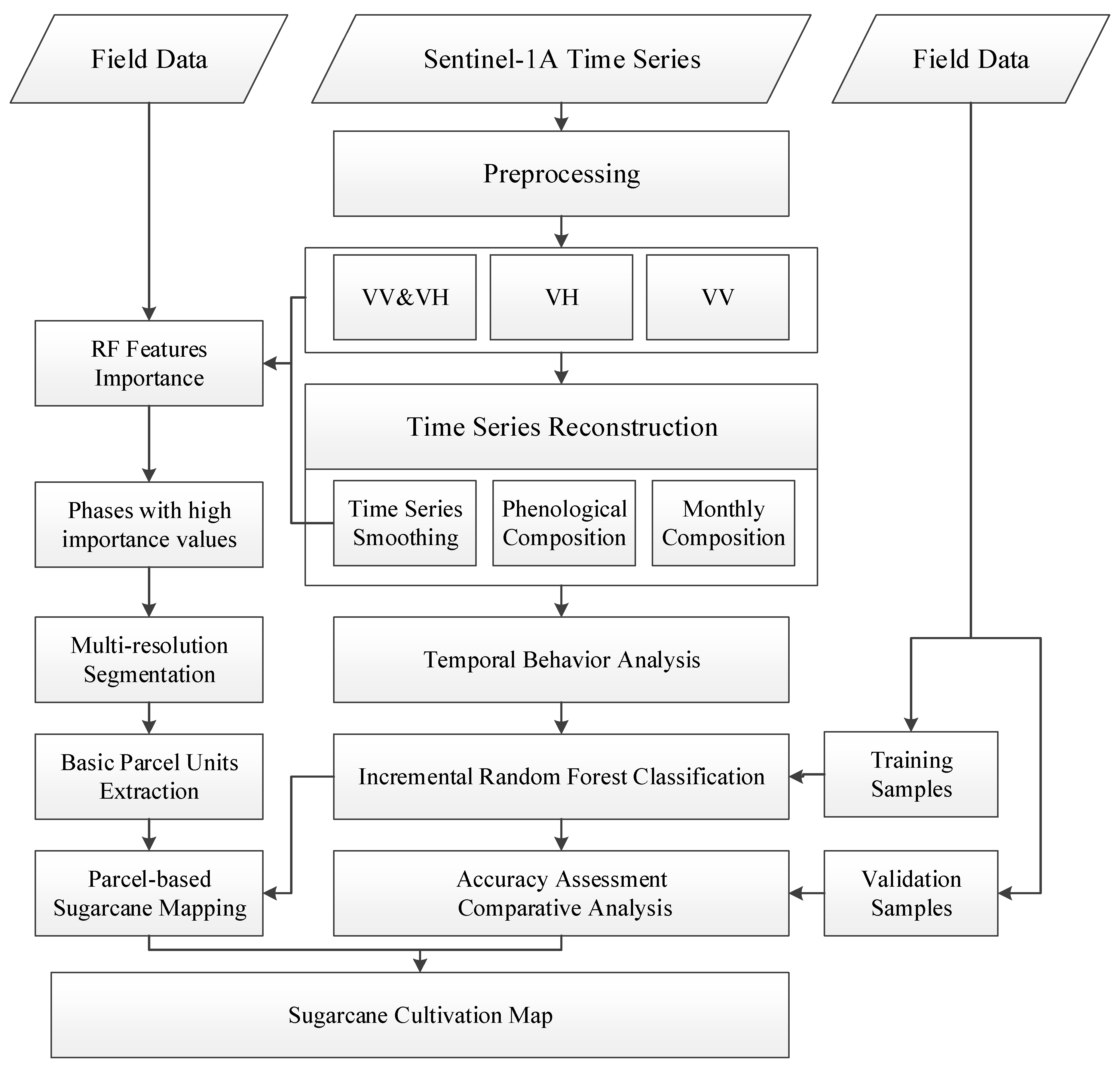
2.3. Experimental Design

In this study, we propose a new application paradigm for sugarcane mapping using only time series SAR data. A comprehensive overview of this study is shown in Figure 3.

First, the time-series smoothing technique and phenology/month-based image compositing approaches were utilized to reconstruct the time-series Sentinel-1A data, based on which the temporal behaviors of sugarcane and other vegetation types were analyzed. Next, using the incremental random forest classifier, the performance of the time-series Sentinel-1A data in sugarcane mapping was assessed for different reconstruction techniques, polarizations, and time ranges. Then, the mean decrease in accuracy (MDA) was used to evaluate the feature importance of each time phase and each polarization mode for sugarcane cultivation discrimination. After that, the phases with high-importance values were selected, and basic parcel units were extracted based on multi-resolution segmentation. At last, the parcel-based classification method, combining time series smoothing SAR data, RF classifier, and basic parcel units, was used to generate a sugarcane extent map.

2.4. Methods

2.4.1. Reconstruction of Time Series Sentinel-1A Data

Speckle noise is the main factor that reduces the quality of SAR images and prevents their efficient agricultural application. In past studies [47,48,49], a multi-channel spatial filter [46] was applied to decrease speckle noise. However, the spatial filter is not capable of preserving the edges of crop parcels. For this reason, we adopted time-series smoothing and multi-temporal compositing techniques to reconstruct the time-series Sentinel-1A data.

To deal with image noise in time-series remote sensing data, many data smoothing techniques have been developed [51,58,59]. In this study, the locally estimated scatterplot smoothing (LOESS) method was applied to the 30 S1 images to mitigate the speckle noise. For LOESS, local polynomial regression was fitted with the weighted least squares method to smooth time-series data [60,61]. It is known that the Savitzky–Golay filtering [62] is very good for filtering time-series data with prominent sharp peaks, while the LOESS filter is very effective when broad signal bands need to be analyzed with robustness [58]. The LOESS filter has two design parameters: polynomial order and window size. Generally, the polynomial order was set to 2–4, and the lower the order is, the smoother the reconstructed time-series data are [50]. Therefore, in this study, the order of the polynomial was set to 2. The size of the filtering window determines the degree of smoothing. In this study, the window size was set to 40 days (covering three phases), and the neighbors were weighted according to their date difference to the fitted value as follows:

$$\omega ={\left(1-{\left({\displaystyle \frac{d}{r}}\right)}^3\right)}^3$$

(1)

where $\omega$ is the tri-cubic weight function, $r$ is the window size of 40 days, and $d$ is the date difference between a given value and the fitted value.

Image compositing is an approach to reduce a series of images into a single image [63]. Multi-temporal compositing was usually used for reducing the influences of clouds and aerosols on optical remote sensing images. Recently, it has been used for Sentinel-1 data to reduce speckle noise [44,64,65]. In this study, we adopted the technique of mean compositing to generate monthly and phenology-based Sentinel-1 composites, respectively. For phenology-based composites, the temporal intervals in the compositing process were set following the timing of the corresponding growth periods, as shown in Section 2.1.

2.4.2. Incremental Classification

To evaluate the effectiveness of the time-series reconstruction technique on sugarcane identification, an incremental classification procedure was used. It has been applied to identify different crop types before the end of the cropping season [38,40,66,67]. This procedure starts with the supervised classification of the first acquired image. In this study, given the diverse planting stage of sugarcane in the test site, we set the acquisition date of the first Sentinel-1A data (4 January 2018) as the start time. Then, a new Sentinel-1A image is stacked to the time series of the previous step, and a new classification is triggered. This process is repeated until all the Sentinel-1A data in 2018 are included.

The supervised classifier used in the incremental classification is the random forest (RF) classifier. RF is a supervised machine learning algorithm for classification and regression. It is an ensemble of decision trees, which are constructed based on the bootstrap aggregated sampling (bagging). RF takes the majority vote of the decision trees for classification. In this study, the randomForest package in the software R 4.4.1 was employed to build the RF model [68]. To evaluate the performance of different polarization modes, the RF-based incremental classification was processed for VH, VV, and VH&VV, respectively.

2.4.3. Feature Importance Assessment

The mean decrease in accuracy (MDA) was used to assess and rank the feature importance for sugarcane discrimination. MDA, also known as permutation importance, is a default output of RF classifier that utilizes permuting out-of-bag samples to estimate the error when excluding a predictor variable from the RF model [69]. An MDA value of zero indicates that there is no connection between the predictor and the response feature, whereas the larger the positive of the MDA value, the more important the feature is for the classification [70].

For this research, MDA was computed in the process of incremental classification when all 30 Sentinel-1A imageries were involved. The testing feature importance score helps to understand which dates and polarization channels are the most important for the discrimination of sugarcane from time-series SAR data.

2.4.4. Parcel-Based Classification Using Multi-Resolution Segmentation

Parcel-based classification can effectively reduce the “salt and pepper” effect following crop classification, especially for time-series SAR images. We used multi-resolution algorithms [71] in eCognition Developer 9.0 [72] to segment images and create homogeneous objects, which is the premise of parcel-based classification [55]. The algorithm is a top-bottom method, achieving image segmentation based on the region of merging technology under the precondition of ensuring minimum average heterogeneity among objects and maximum homogeneity among the internal pixels of the objects [72]. It is regarded as one of the most successful methods to produce meaningful image objects [73].

As Sentinel-1A data with adjacent dates have a strong similarity, in this study, we selected three images with nonadjacent phases as the input of multi-resolution segmentation. The phases (12 March, 29 April, and 4 June) were selected in terms of the feature importance shown in Section 3.2. The parameters of scale, shape, and compactness influence the segmentation effect. In this paper, the identification of homogeneous sugarcane parcels was carried out through a supervised iterative process by tuning the three parameters. The optimum segmentation effect was identified with a scale of 50, compactness 0.6, and shape 0.6.

The pixel-wise classification results were integrated with the multi-resolution segmentation results. For each segmented polygon parcel unit, the pixel numbers of sugarcane and non-sugarcane were recorded as $m$ and $n$, respectively. If $m\ge n$, the parcel polygon was labeled as sugarcane field, otherwise, non-sugarcane field.

2.4.5. Accuracy Assessment

To assess the performance of time-series Sentinel-1 images on sugarcane cultivation mapping, the confusion matrix was calculated based on the 484 validation samples for each classification result in Section 2.4.2. Four indicators were calculated by the confusion matrix, including overall accuracy (OA), kappa coefficient (Kappa), user’s accuracy (UA), and producer’s accuracy (PA). These four indicators together provide a comprehensive classification validation framework, allowing for the evaluation of classification model performance from different perspectives to ensure the reliability and accuracy of the classification results.

3. Results

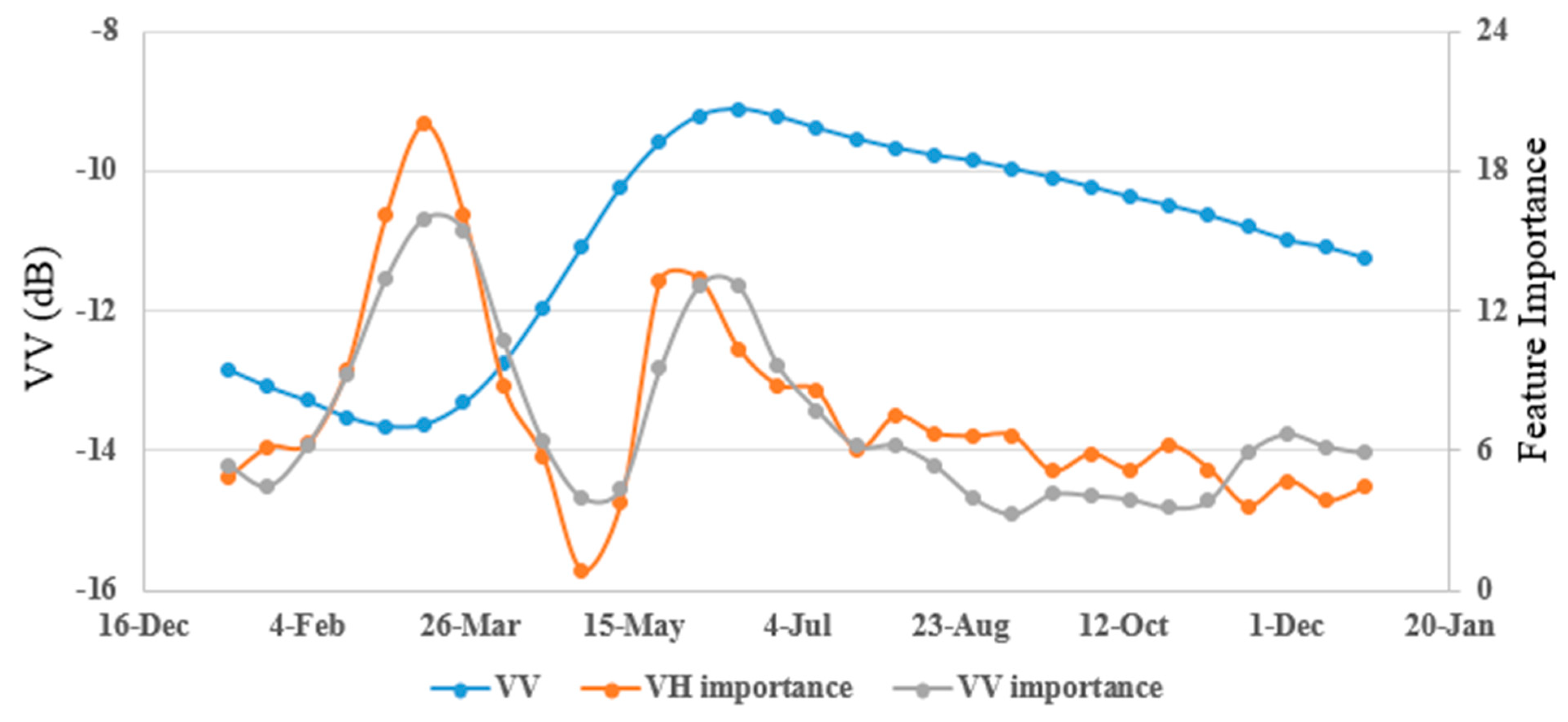
3.1. Temporal Behavior of SAR Backscattering over Vegetation

The temporal profiles of sugarcane and other 11 typical vegetations were plotted based on the Sentinel-1A backscattering coefficient (${\sigma }^0$ in dB), as shown in Figure 4. The blue and orange curves represent the VV and VH polarization, respectively. The 11 typical vegetations included banana, paddy rice, pineapple, papaw, sweet potato, dragon fruit, mango, eucalyptus, sisal, longan, and litchi. It should be noted that the curves in Figure 4 were based on the LOESS filter of Sentinel-1A data rather than the original data.

As shown in Figure 4a, for sugarcane, the temporal profile of VV and VH polarization had similar changing characteristics. The characteristics were related to sugarcane growth periods: (1) the minimum backscatter coefficients occurred during the sugarcane seedling period (late March to early April). The minimum values of VV and VH polarization were about −14 db and −21 db, respectively; (2) during the tillering period (from early April to late May), the backscatter coefficients increased sharply. The maximum values of VV and VH polarization (−9 db and −15 db) occurred in the late tillering period; (3) during the grand growth period (from June to October), the backscatter coefficients decreased slowly; (4) during the mature period (after October), the backscatter coefficients remained basically unchanged.

Significant differences can be observed between sugarcane and other vegetation: (1) for dragon fruit, eucalyptus, sisal, longan, and litchi, the backscatter coefficients fluctuated, rising and falling slightly throughout the year; (2) for paddy rice, pineapple, papaw, sweet potato, and mango, the periods of sharp changes were different from sugarcane; (3) for banana, the backscatter coefficients were much higher than sugarcane.

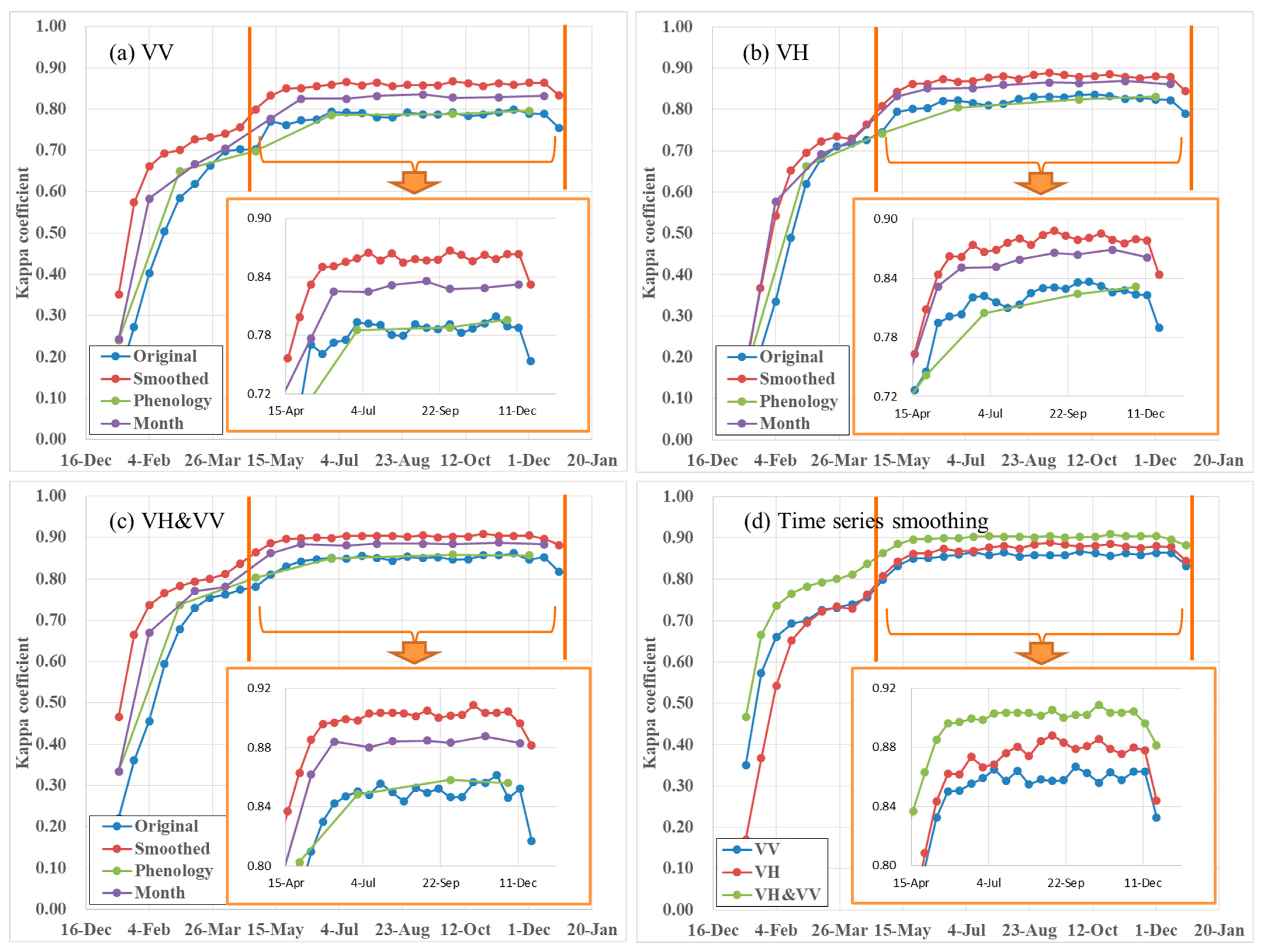
3.2. Performance of Time Series Smoothing

Figure 5 shows the comparison of the time series of smoothed data based on the LOESS filter (blue curve) and the original data (red curve). The mean and standard deviation were calculated based on the 1134 training samples. The effect of time series smoothing can be observed as follows: (1) For the mean value of VV (or VH) polarization as shown in Figure 5a,c, the LOESS-smoothed data was much smoother than the original data. The blue curves were almost unaffected by speckle noise, and they can be regarded as standard curves of sugarcane samples; (2) for the standard deviation of VV (or VH) polarization as shown in Figure 5b,d, the LOESS-smoothed data was smaller than the original data, and the difference was about 1 dB. It should be noted that the higher standard deviation at the beginning (from January to February) and end (from November to December) of the year was from when the harvest period of sugarcane began in late October and lasted until March of the following year, and the specific harvest time was arranged according to the sugarcane mill’s plan.

3.3. Feature Importance

Figure 6 shows the feature importance for the sugarcane discrimination that employed both VV and VH polarizations. The blue curve was the standard sugarcane temporal profile of the LOESS-smoothed VV polarization in Figure 5a. The orange and gray curves demonstrated the feature importance of each temporal for VH and VV polarizations, respectively. The temporal feature importance of the VH and VV polarizations were similar. There was no significant difference between VV and VH polarizations. Their correlation coefficient was as high as 0.89. Although the VH polarization on 12 March obtained the highest importance score, it was hard to draw a conclusion about which polarization was better for sugarcane identification. The most important phase was on 12 March. For VH and VV polarizations, the feature importance was 20.04 and 15.97, respectively. The second most important phase was on 4 June. For VH and VV polarizations, the feature importance was 13.39 and 13.05, respectively. The tillering period (from late March to late May) and grand growth period (from June to October) showed low importance values.

3.4. Comparison of Classification Accuracy

Figure 7 shows the sugarcane mapping Kappa coefficient with the incremental image acquisition date based on VV polarization (Figure 7a), VH polarization (Figure 7b), and VH&VV (Figure 7c), respectively. In these three sub-figures, four kinds of time series reconstruction methods were compared: (1) original time series data (blue); (2) smoothed time series data with LOESS filter (red); (3) phenology-based compositing data (green); and (4) monthly based compositing data (purple). Figure 7d shows the comparison of different polarization modes based on smoothed time series data. To clearly show the difference between them, the data between April and December were enlarged at the lower right corner of each sub-figure.

As shown in Figure 7a–c, for all three polarization modes, the smoothed time series data with LOESS filter performed best, followed by the monthly based compositing data and the original time series data, and the phenology-based compositing data ranked last. Compared to the original time series data, the LOESS time series filter can improve the Kappa coefficient by about 0.06.

Among the three polarization modes in Figure 7d, the VH&VV polarization performed best, followed by the VH polarization, and the VV polarization ranked last. The VH&VV polarization outperformed VH polarization by about 0.05 (Kappa coefficient). Before May, the performance of VH and VV polarization was not much different; however, during May and October, VH polarization gradually performed better than VV polarization, and the maximum difference (0.06) was in mid-September.

In terms of temporal behaviors, before mid-April, the Kappa coefficient was lower than 0.80; then, during mid-April and early-July, the Kappa coefficient gradually increased to the highest level. After July, the Kappa coefficient profiles exhibited no further improvement and fluctuated at high levels.

Table 1. Confusion matrix for the classification accuracy assessment of sugarcane.

	Pixel-Based					Parcel-Based
VV		Sugarcane	Other	Total	UA		Sugarcane	Other	Total	UA
	Sugarcane	152	13	165	92.12%	Sugarcane	157	11	168	93.45%
	Other	18	303	321	94.39%	Other	13	305	318	95.91%
	Total	170	316	486		Total	170	316	486
	PA	89.41%	95.89%			PA	92.35%	97.52%
	OA: 93.62%		Kappa: 0.86			OA: 95.06%		Kappa: 0.89
VH		Sugarcane	Other	Total	UA		Sugarcane	Other	Total	UA
	Sugarcane	155	11	166	93.37%	Sugarcane	158	9	167	94.61%
	Other	15	305	320	95.31%	Other	12	307	319	96.24%
	Total	170	316	486		Total	170	316	486
	PA	91.18%	96.52%			PA	92.94%	97.15%
	OA: 94.65%		Kappa: 0.88			OA: 95.68%		Kappa: 0.90
VV & VH		Sugarcane	Other	Total	UA		Sugarcane	Other	Total	UA
	Sugarcane	158	10	168	94.05%	Sugarcane	159	8	167	95.21%
	Other	12	306	318	96.23%	Other	11	308	319	96.55%
	Total	170	316	486		Total	170	316	486
	PA	92.94%	96.84%			PA	93.53%	97.47%
	OA: 95.47%		Kappa: 0.90			OA: 96.09%		Kappa: 0.91

shows the confusion matrix for the sugarcane classification accuracy assessment. The classification results were based on the smoothed time series data of VV, VH, and VH&VV polarization modes, respectively. The left column was for the pixel-based classification, and the right column was for the parcel-based classification.

As shown in Table 1, for the three polarization modes, compared with the pixel-based classification method, the parcel-based method can effectively improve the classification accuracy. Take VV polarization for example, the OA changed from 93.62% to 95.06%, and the Kappa coefficient changed from 0.86 to 0.89. When the VH&VV polarization mode was combined with the parcel-based classification method, the classification accuracy reached the highest with the OA of 96.09% and the Kappa coefficient of 0.91.

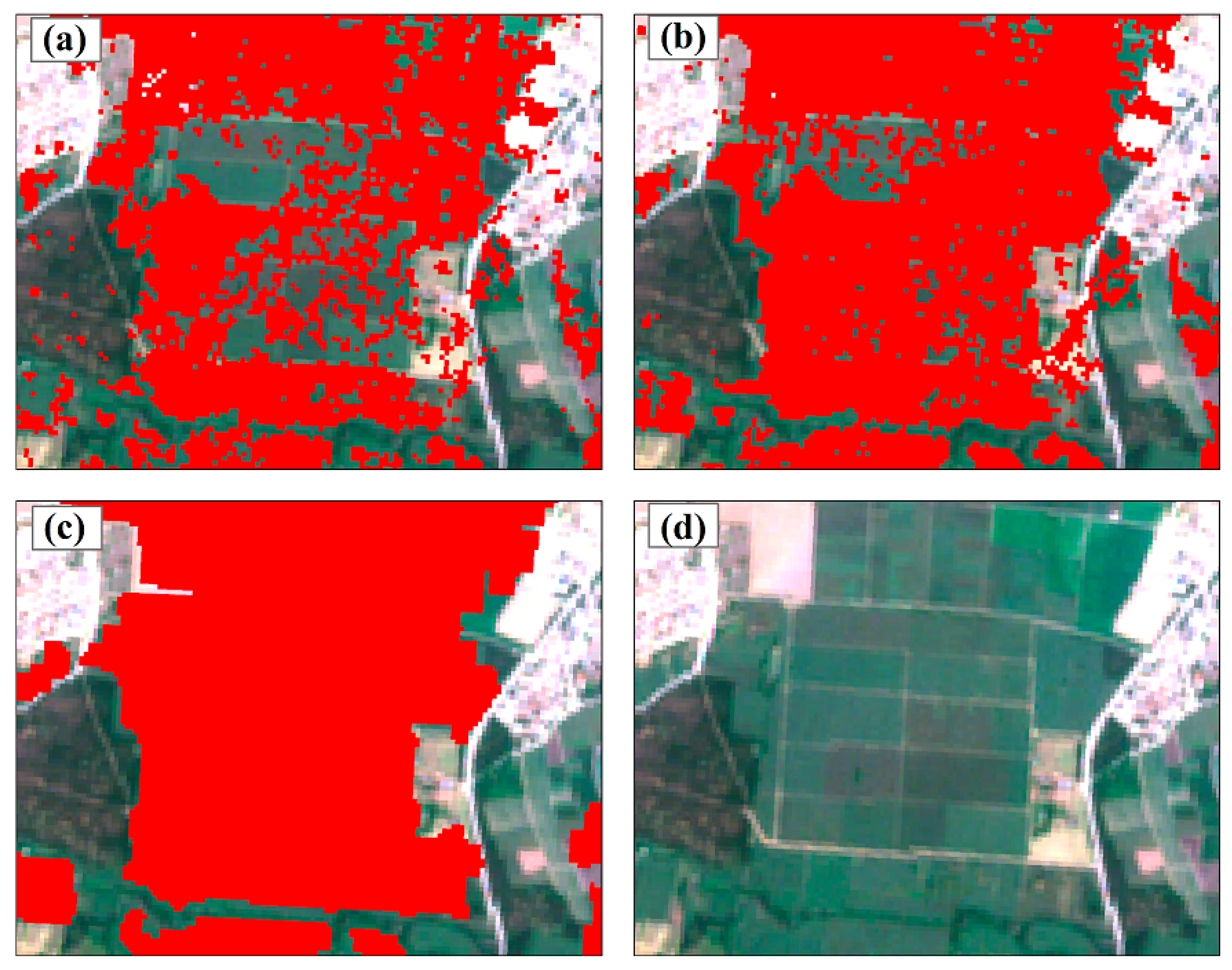
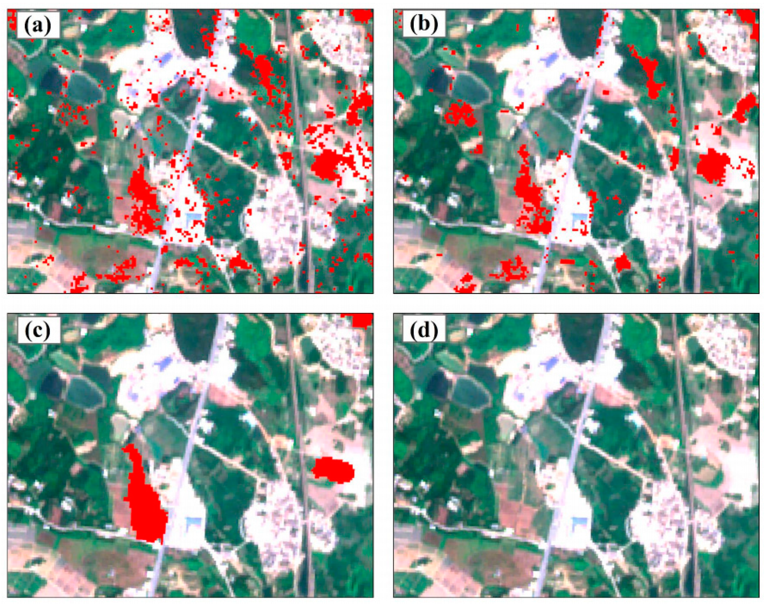
3.5. Sugarcane Mapping Results

Figure 8 shows the sugarcane mapping results in Suixi County using different methods. Comparing the three subfigures, the sugarcane extent maps showed similar spatial distribution characteristics. The sugarcane was mainly planted in central Suixi, while in the southwest and northeast, sugarcane was planted sporadically and was less distributed. However, obvious “salt and pepper” noise can be seen in Figure 8a,b. In Figure 8c, the “salt and pepper” noise in the sugarcane extent map had been significantly improved. To better show the effect of the parcel-based method on noise removal, three ROIs (in Figure 8c) were enlarged in Figure 9, Figure 10 and Figure 11. The base map was a Sentinel-2 RGB composite image acquired on 3 January 2018.

In Figure 9, Figure 10 and Figure 11, comparing sub-figures (a)–(c), it can be seen that there were many small spots in the pixel-based results using the original data. When the smoothed time series data was used, these small spots were significantly reduced, and after parcel-based classification, these spots were almost completely eliminated. Obviously, most of these spots were incorrectly classified into sugarcane class, as their areas and distributions were very inconsistent with the actual planting pattern of sugarcane. In particular, in sub-figure (c), all non-vegetation spots, such as roads, built-up areas, and water bodies, were removed.

In addition, the completeness of the sugarcane plot was gradually improved. In sub-figure (a), the interior of the sugarcane plot was relatively rough, and nearly half of the pixels were incorrectly classified into non-sugarcane class. When the smoothed data were used, more than 80% of the pixels in the sugarcane plot were correctly classified, and after parcel-based classification, the sugarcane plots could be completely identified.

4. Discussion

4.1. New Application Paradigm of Time Series SAR Data for Sugarcane Mapping

The all-weather observation capability of SAR combined with time series data held great potential in sugarcane mapping. However, the “salt and pepper” effects in sugarcane maps caused by the inherent speckle noise of SAR images greatly reduced their application potential. To overcome the effect of SAR speckle noise, this study explored a new application paradigm of time series SAR data for sugarcane mapping. First, the time series smoothing technique was exploited to reduce SAR noise in the time domain. Then, basic parcel units were obtained only based on multi-temporal SAR images. Finally, the parcel-based classification method was used to eliminate unreasonable spots in the spatial domain.

Briefly, the application paradigm proposed in this paper benefited in two ways. First, the process of time series smoothing was not only helpful in suppressing noise in the time dimension (Figure 5a,c) but also enhanced the compactness of sugarcane samples in the space dimension (Figure 5b,d). The enhanced compactness indicated a smaller intra-class distance and an improved capacity for accurate classification [74]. Results in Figure 7 showed that compared to the original data, the smoothed time series data can improve the Kappa coefficient by about 0.06, and this improvement in accuracy occurred throughout all phases of the year. Classification maps in Figure 8, Figure 9, Figure 10 and Figure 11 showed that the smoothing process can dramatically reduce the “salt and pepper” spots and improve the rationality of sugarcane mapping. In this study, we also tried some other reconstruction techniques of time series data, such as multi-time composition and phenology-based aggregation, which have been used to reduce SAR speckle noise [65,75]. However, their performance was worse than the smoothing technique in terms of classification accuracy, and the phenology-based aggregation data was only equivalent to the original data. In recent years, time series smoothing techniques have been applied to SAR data in sunflower monitoring and paddy rice mapping [76,77], and we believe that time series smoothing will be a necessary preprocessing step in time series SAR agricultural monitoring in the future. Second, the proposed paradigm was based only on SAR data without any additional cropland (or urban and water) map or optical data, which is different from the existing methods using SAR images for sugarcane mapping [20,38,39,78,79]. Although the parcel-based method showed a limited performance in improving classification accuracy, it eliminated the non-vegetation spots and filled the hollow spots within large sugarcane patches in sugarcane mapping results completely, which is more in line with the actual distribution characteristics of sugarcane (Figure 9, Figure 10 and Figure 11). In this study, the RF classifier was exploited at the pixel level, and the parcel units were used to determine whether the parcel unit was dominated by sugarcane. In this manner, there is no need to calculate the mean value of each parcel for every phase, and it was suitable for single-crop type mapping [55]. Different from the previous studies [45,49,55,57], we obtained the basic parcel units based on SAR data. To avoid the impact of too much temporal data on the size of parcel units, only three temporal SAR data were selected, which were based on the temporal importance in RF MDA ranking.

4.2. Temporal Importance and Early Season Mapping

The temporal importance of time series Sentinel-1 data for sugarcane mapping partly agreed with previous studies [36,38]. In our study, as shown in Figure 6, the image acquisition dates with high feature importance were 12 March and 4 June. In a previous study [38], the image acquisition dates with high importance value were 10 March, 3 April, 2 June, 1 August, and 21 February. Among the five dates, 10 March and 2 June were approximately to the 12 March and 4 June in our study. The date 12 March was during the sugarcane germination period when sugarcane had just been planted or was about to be planted, and the predominant land cover type was bare soil. The date 4 June was at the end of the tillering period and the beginning of the grand growth period, when the height of the sugarcane stem was about 140 cm, the number of leaves increased to about 13, and the leaves basically covered the ground [33,36]. For the other three dates (3 April, 1 August, and 21 February), there was no corresponding date in our study. This was mainly due to the difference in the classification system. In the previous study [38], the classification system included five local vegetation types: sugarcane, eucalyptus, paddy rice, banana, and pineapple. In our study, the non-sugarcane samples included artificial, wetland, and other 11 vegetation types.

In [36], the middle tillering period (late April) was regarded as suitable and might be optimal for sugarcane mapping. However, in our study, the tillering period (from late March to late May) showed low importance values. There are two reasons for this difference. First, the different features for sugarcane mapping. In [36], the sugarcane mapping was based on polarimetric parameters (scattering angle $\alpha$ and polarization entropy $H$) of X-band TerraSAR data, while this study used the backscattering coefficient ${\delta }^{\mathsf{0}}$ of C-band Sentinel-1A data. Second, the different phases of image acquisition. In [36], three TerraSAR-X images were collected in the early, middle, and late tillering periods, while in this study, 30 Sentinel-1A images were acquired throughout the entire growing period of sugarcane.

Early season identification of sugarcane is crucial for sugar yield estimation and the future market. Combining the temporal importance in Figure 6 and the incremental classification accuracy in Figure 7, the appropriate time for early-season sugarcane identification was mid-June. After this time, any date showed low importance values, and for the VV, VH, and VH&VV polarization modes, a longer time series provided no further improvement in classification performance. The date of mid-June in our study was one and a half months earlier than the result in [2], which was three months before sugarcane harvest. We believe that this difference was generated due to the time-series smoothing of Sentinel-1A data, that is, the process of time-series smoothing can advance the date of early season sugarcane identification.

4.3. Limitations and Prospects

Although the new paradigm in this study was free from the influence of the cloudy and rainy weather, it still cannot avoid the influence of the diversity of sugarcane cultivation patterns. As stated in [36], the sugarcane cultivations in the study area might be in different planting stages or growing periods. Thus, the status of the sugarcane was not necessarily specific. Moreover, the diversity of sugarcane-planting row directions and sugarcane plot radar incidence angles in the Sentinel-1A coordinate system can increase the variability of the scattering coefficient in each time phase. The effect of sugarcane-planting row directions on ALOS/PALSAR satellite images has been investigated in [80], while the effect of sugarcane plot radar incidence angle has not yet been mentioned. We found the same sugarcane plot showed different backscattering coefficients ${\delta }^{\mathsf{0}}$ in adjacent granules (with relative orbit number/slice numbers of 157/2 and 84/2, respectively) throughout the whole sugarcane growth cycle. For VV polarization, ${\delta }^{\mathsf{0}}$ values with a low incidence angle (about 30°) were 2~4 dB higher than those with a high incidence angle (about 45°).

These factors reduced the regional transferability of the sugarcane identification model. We applied the sugarcane identification model to the entirety of Zhanjiang City, which was the superior administrative district of Suixi County, and the overall accuracy was reduced by about 10%. Therefore, although the new paradigm in this study can be used in large cloudy and rainy areas to map sugarcane cultivation due to its capability of eliminating the impact of SAR noise, to achieve high accuracy of sugarcane mapping in large areas, a large number of samples are still needed to drive the classification model and eliminate the influence of sugarcane planting patterns, radar incidence angle, and other factors.

In the future, the paradigm can be further used to extract the sugarcane growth cycle and estimate phenology periods. On this basis, we will try to establish a SAR-based sugarcane index similar to the paddy rice index in [81] and introduce deep learning models as in [82,83] to improve regional transferability.

Additionally, we will compare various time-series smoothing methods to determine the most suitable time-series filtering method for Sentinel-1 data in sugarcane identification. This will be applied to monitor different phenological stages of sugarcane, similar to the experiments conducted on MODIS NDVI data in [58].

5. Conclusions

Knowledge of the spatial extent of sugarcane cultivation is significant to ensure the sustainability of the sugarcane industry. In this study, we proposed a new paradigm for sugarcane cultivation mapping based on time series SAR data. Unlike previous studies, the proposed paradigm was based only on SAR data without any additional map or optical data. The LOESS smoothing technique was exploited to reduce SAR noise in the time domain, and the parcel-based classification method was used to remove the “pepper and salt” effect in the space domain.

The results indicate that the new paradigm was successful in generating a highly precise sugarcane map, with an overall accuracy of 96.09% and a Kappa coefficient of 0.91. The new paradigm of parcel-based sugarcane mapping using smoothed time series SAR data has several advantages: (1) it does not need any land cover map or optical data; (2) it can enhance the compactness of sugarcane samples; (3) it eliminates the non-vegetation spots in sugarcane maps completely; (4) it can improve the completeness of sugarcane plots; and (5) it advances the date for early season sugarcane identification by about one and a half months. Therefore, the proposed new paradigm offers a high level of practicality for mapping sugarcane in large areas, particularly in cloudy areas where optical remote sensing data is frequently unavailable.

References

1. Sindhu, R.; Gnansounou, E.; Binod, P.; Pandey, A. Bioconversion of sugarcane crop residue for value added products—An overview. Renew. Energy 2016, 98, 203–215. [Google Scholar] [CrossRef]
2. Cardona, C.A.; Quintero, J.A.; Paz, I.C. Production of bioethanol from sugarcane bagasse: Status and perspectives. Bioresour. Technol. 2010, 101, 4754–4766. [Google Scholar] [CrossRef]
3. Pan, S.; Zabed, H.M.; Wei, Y.; Qi, X. Technoeconomic and environmental perspectives of biofuel production from sugarcane bagasse: Current status, challenges and future outlook. Ind. Crops Prod. 2022, 188, 115684. [Google Scholar] [CrossRef]
4. OECD-FAO. OECD-FAO Agricultural Outlook 2022–2031; Food & Agriculture Org.: Rome, Italy, 2022. [Google Scholar]
5. Cheavegatti-Gianotto, A.; de Abreu, H.M.; Arruda, P.; Bespalhok Filho, J.C.; Burnquist, W.L.; Creste, S.; di Ciero, L.; Ferro, J.A.; de Oliveira Figueira, A.V.; de Sousa Filgueiras, T.; et al. Sugarcane (Saccharum x officinarum): A reference study for the regulation of genetically modified cultivars in brazil. Trop. Plant Biol. 2011, 4, 62–89. [Google Scholar] [CrossRef]
6. Som-ard, J.; Atzberger, C.; Izquierdo-Verdiguier, E.; Vuolo, F.; Immitzer, M. Remote sensing applications in sugarcane cultivation: A review. Remote Sens. 2021, 13, 4040. [Google Scholar] [CrossRef]
7. El Chami, D.; Daccache, A.; El Moujabber, M. What are the impacts of sugarcane production on ecosystem services and human well-being? A review. Ann. Agric. Sci. 2020, 65, 188–199. [Google Scholar] [CrossRef]
8. Dinesh Babu, K.S.; Janakiraman, V.; Palaniswamy, H.; Kasirajan, L.; Gomathi, R.; Ramkumar, T.R. A short review on sugarcane: Its domestication, molecular manipulations and future perspectives. Genet. Resour. Crop. Evol. 2022, 69, 2623–2643. [Google Scholar] [CrossRef] [PubMed]
9. Cock, J. Sugarcane growth and development. Int. Sugar J. 2003, 105, 540–552. [Google Scholar]
10. FAOSTAT. Sugarcane Production in 2020, Crops/Regions/World List/Production Quantity (Pick Lists); FAOSTAT: Rome, Italy, 2022. [Google Scholar]
11. Defante, L.R.; Vilpoux, O.F.; Sauer, L. Rapid expansion of sugarcane crop for biofuels and influence on food production in the first producing region of brazil. Food Policy 2018, 79, 121–131. [Google Scholar] [CrossRef]
12. Adami, M.; Rudorff, B.F.T.; Freitas, R.M.; Aguiar, D.A.; Sugawara, L.M.; Mello, M.P. Remote sensing time series to evaluate direct land use change of recent expanded sugarcane crop in brazil. Sustainability 2012, 4, 574–585. [Google Scholar] [CrossRef]
13. Zheng, Y.; dos Santos Luciano, A.C.; Dong, J.; Yuan, W. High-resolution map of sugarcane cultivation in brazil using a phenology-based method. Earth Syst. Sci. Data 2022, 14, 2065–2080. [Google Scholar] [CrossRef]
14. Cherubin, M.R.; Carvalho, J.L.; Cerri, C.E.; Nogueira, L.A.; Souza, G.M.; Cantarella, H. Land use and management effects on sustainable sugarcane-derived bioenergy. Land 2021, 10, 72. [Google Scholar] [CrossRef]
15. Silalertruksa, T.; Gheewala, S.H. Land-water-energy nexus of sugarcane production in thailand. J. Clean. Prod. 2018, 182, 521–528. [Google Scholar] [CrossRef]
16. Jaiswal, D.; De Souza, A.P.; Larsen, S.; LeBauer, D.S.; Miguez, F.E.; Sparovek, G.; Bollero, G.; Buckeridge, M.S.; Long, S.P. Brazilian sugarcane ethanol as an expandable green alternative to crude oil use. Nat. Clim. Chang. 2017, 7, 788–792. [Google Scholar] [CrossRef]
17. Zhang, H.; Anderson, R.G.; Wang, D. Satellite-based crop coefficient and regional water use estimates for hawaiian sugarcane. Field Crops Res. 2015, 180, 143–154. [Google Scholar] [CrossRef]
18. Mello, F.F.C.; Cerri, C.E.P.; Davies, C.A.; Holbrook, N.M.; Paustian, K.; Maia, S.M.F.; Galdos, M.V.; Bernoux, M.; Cerri, C.C. Payback time for soil carbon and sugar-cane ethanol. Nat. Clim. Chang. 2014, 4, 605–609. [Google Scholar] [CrossRef]
19. Loarie, S.R.; Lobell, D.B.; Asner, G.P.; Mu, Q.; Field, C.B. Direct impacts on local climate of sugar-cane expansion in Brazil. Nat. Clim. Chang. 2011, 1, 105–109. [Google Scholar] [CrossRef]
20. Wang, J.; Xiao, X.; Liu, L.; Wu, X.; Qin, Y.; Steiner, J.L.; Dong, J. Mapping sugarcane plantation dynamics in Guangxi, China, by time series sentinel-1, sentinel-2 and landsat images. Remote Sens. Environ. 2020, 247, 111951. [Google Scholar] [CrossRef]
21. Abdel-Rahman, E.M.; Ahmed, F.B. The application of remote sensing techniques to sugarcane (Saccharum spp. Hybrid) production: A review of the literature. Int. J. Remote Sens. 2008, 29, 3753–3767. [Google Scholar] [CrossRef]
22. Zhan, P.; Zhu, W.; Li, N. An automated rice mapping method based on flooding signals in synthetic aperture radar time series. Remote Sens. Environ. 2021, 252, 112112. [Google Scholar] [CrossRef]
23. Mateo-Sanchis, A.; Piles, M.; Muñoz-Marí, J.; Adsuara, J.E.; Pérez-Suay, A.; Camps-Valls, G. Synergistic integration of optical and microwave satellite data for crop yield estimation. Remote Sens. Environ. 2019, 234, 111460. [Google Scholar] [CrossRef] [PubMed]
24. Joshi, N.; Baumann, M.; Ehammer, A.; Fensholt, R.; Grogan, K.; Hostert, P.; Jepsen, M.R.; Kuemmerle, T.; Meyfroidt, P.; Mitchard, E.T.A.; et al. A review of the application of optical and radar remote sensing data fusion to land use mapping and monitoring. Remote Sens. 2016, 8, 70. [Google Scholar] [CrossRef]
25. de Souza, C.H.W.; Cervi, W.R.; Brown, J.C.; Rocha, J.V.; Lamparelli, R.A.C. Mapping and evaluating sugarcane expansion in Brazil’s savanna using modis and intensity analysis: A case-study from the state of tocantins. J. Land Use Sci. 2017, 12, 457–476. [Google Scholar] [CrossRef]
26. Xavier, A.C.; Rudorff, B.F.T.; Shimabukuro, Y.E.; Berka, L.M.S.; Moreira, M.A. Multi-temporal analysis of modis data to classify sugarcane crop. Int. J. Remote Sens. 2006, 27, 755–768. [Google Scholar] [CrossRef]
27. Singh, R.; Patel, N.R.; Danodia, A. Deriving phenological metrics from landsat-oli for sugarcane crop type mapping: A case study in North India. J. Indian Soc. Remote Sens. 2022, 50, 1021–1030. [Google Scholar] [CrossRef]
28. dos Luciano, A.C.; Picoli, M.C.A.; Rocha, J.V.; Duft, D.G.; Lamparelli, R.A.C.; Leal, M.R.L.V.; Le Maire, G. A generalized space-time obia classification scheme to map sugarcane areas at regional scale, using landsat images time-series and the random forest algorithm. Int. J. Appl. Earth Obs. Geoinf. 2019, 80, 127–136. [Google Scholar] [CrossRef]
29. Zhou, Z.; Huang, J.; Wang, J.; Zhang, K.; Kuang, Z.; Zhong, S.; Song, X. Object-oriented classification of sugarcane using time-series middle-resolution remote sensing data based on adaboost. PLoS ONE 2015, 10, e0142069. [Google Scholar] [CrossRef]
30. Wang, J.; Huang, J.; Wang, L.; Hu, Y.; Han, P.; Huang, W. Identification of sugarcane based on object-oriented analysis using time-series HJ CCD data. Trans. Chin. Soc. Agric. Eng. 2014, 30, 145–151. [Google Scholar]
31. Zheng, Y.; Li, Z.; Pan, B.; Lin, S.; Dong, J.; Li, X.; Yuan, W. Development of a phenology-based method for identifying sugarcane plantation areas in china using high-resolution satellite datasets. Remote Sens. 2022, 14, 1274. [Google Scholar] [CrossRef]
32. Wang, M.; Liu, Z.; Ali Baig, M.H.; Wang, Y.; Li, Y.; Chen, Y. Mapping sugarcane in complex landscapes by integrating multi-temporal sentinel-2 images and machine learning algorithms. Land Use Policy 2019, 88, 104190. [Google Scholar] [CrossRef]
33. Lin, H.; Chen, J.; Pei, Z.; Zhang, S.; Hu, X. Monitoring sugarcane growth using envisat asar data. IEEE Trans. Geosci. Remote Sens. 2009, 47, 2572–2580. [Google Scholar] [CrossRef]
34. Baghdadi, N.; Boyer, N.; Todoroff, P.; El Hajj, M.; Bégué, A. Potential of sar sensors TerraSAR-X, ASAR/ENVISAT and PALSAR/ALOS for monitoring sugarcane crops on reunion island. Remote Sens. Environ. 2009, 113, 1724–1738. [Google Scholar] [CrossRef]
35. Baghdadi, N.; Cresson, R.; Todoroff, P.; Moinet, S. Multitemporal observations of sugarcane by TerraSAR-X images. Sensors 2010, 10, 8899–8919. [Google Scholar] [CrossRef]
36. Li, H.; Chen, J.; Liang, S.; Li, Q. Sugarcane mapping in tillering period by quad-polarization TerraSAR-X data. IEEE Geosci. Remote Sens. Lett. 2015, 12, 993–997. [Google Scholar]
37. Li, H.; Han, Y.; Chen, J. Capability of multidate RADARSAT-2 data to identify sugarcane lodging. J. Appl. Remote Sens. 2019, 13, 044514. [Google Scholar] [CrossRef]
38. Jiang, H.; Li, D.; Jing, W.; Xu, J.; Huang, J.; Yang, J.; Chen, S. Early season mapping of sugarcane by applying machine learning algorithms to sentinel-1a/2 time series data: A case study in Zhanjiang city, China. Remote Sens. 2019, 11, 861. [Google Scholar] [CrossRef]
39. Sreedhar, R.; Varshney, A.; Dhanya, M. Sugarcane crop classification using time series analysis of optical and sar sentinel images: A deep learning approach. Remote Sens. Lett. 2022, 13, 812–821. [Google Scholar] [CrossRef]
40. Zhao, H.; Chen, Z.; Jiang, H.; Jing, W.; Sun, L.; Feng, M. Evaluation of three deep learning models for early crop classification using sentinel-1a imagery time series—A case study in Zhanjiang, China. Remote Sens. 2019, 11, 2673. [Google Scholar] [CrossRef]
41. Yuan, J.; Lv, X.; Li, R. A speckle filtering method based on hypothesis testing for time-series sar images. Remote Sens. 2018, 10, 1383. [Google Scholar] [CrossRef]
42. Jong-Sen, L. Speckle suppression and analysis for synthetic aperture radar images. Opt. Eng. 1986, 25, 255636. [Google Scholar]
43. Satalino, G.; Balenzano, A.; Mattia, F.; Davidson, M.W.J. C-band sar data for mapping crops dominated by surface or volume scattering. IEEE Geosci. Remote Sens. Lett. 2014, 11, 384–388. [Google Scholar] [CrossRef]
44. Luo, C.; Qi, B.; Liu, H.; Guo, D.; Lu, L.; Fu, Q.; Shao, Y. Using time series sentinel-1 images for object-oriented crop classification in google earth engine. Remote Sens. 2021, 13, 561. [Google Scholar] [CrossRef]
45. Beriaux, E.; Jago, A.; Lucau-Danila, C.; Planchon, V.; Defourny, P. Sentinel-1 time series for crop identification in the framework of the future cap monitoring. Remote Sens. 2021, 13, 2785. [Google Scholar] [CrossRef]
46. Quegan, S.; Yu, J.J. Filtering of multichannel sar images. IEEE Trans. Geosci. Remote Sens. 2001, 39, 2373–2379. [Google Scholar] [CrossRef]
47. Schlund, M.; Erasmi, S. Sentinel-1 time series data for monitoring the phenology of winter wheat. Remote Sens. Environ. 2020, 246, 111814. [Google Scholar] [CrossRef]
48. Nasrallah, A.; Baghdadi, N.; El Hajj, M.; Darwish, T.; Belhouchette, H.; Faour, G.; Darwich, S.; Mhawej, M. Sentinel-1 data for winter wheat phenology monitoring and mapping. Remote Sens. 2019, 11, 2228. [Google Scholar] [CrossRef]
49. Bazzi, H. Mapping paddy rice using sentinel-1 sar time series in Camargue, France. Remote Sens. 2019, 11, 887. [Google Scholar] [CrossRef]
50. Li, S.; Xu, L.; Jing, Y.; Yin, H.; Li, X.; Guan, X. High-quality vegetation index product generation: A review of NDVI time series reconstruction techniques. Int. J. Appl. Earth Obs. Geoinf. 2021, 105, 102640. [Google Scholar] [CrossRef]
51. Geng, L.; Ma, M.; Wang, X.; Yu, W.; Jia, S.; Wang, H. Comparison of eight techniques for reconstructing multi-satellite sensor time-series NDVI data sets in the Heihe River Basin, China. Remote Sens. 2014, 6, 2024–2049. [Google Scholar] [CrossRef]
52. Malhi, R.K.M.; Kiran, G.S.; Shah, M.N.; Mistry, N.V.; Bhavsar, V.H.; Singh, C.P.; Bhattarcharya, B.K.; Townsend, P.A.; Mohan, S. Applicability of smoothing techniques in generation of phenological metrics of Tectona grandis L. Using NDVI time series data. Remote Sens. 2021, 13, 3343. [Google Scholar] [CrossRef]
53. Soudani, K.; Delpierre, N.; Berveiller, D.; Hmimina, G.; Vincent, G.; Morfin, A.; Dufrêne, É. Potential of c-band synthetic aperture radar sentinel-1 time-series for the monitoring of phenological cycles in a deciduous forest. Int. J. Appl. Earth Obs. Geoinf. 2021, 104, 102505. [Google Scholar] [CrossRef]
54. Stendardi, L.; Karlsen, S.R.; Niedrist, G.; Gerdol, R.; Zebisch, M.; Rossi, M.; Notarnicola, C. Exploiting time series of sentinel-1 and sentinel-2 imagery to detect meadow phenology in mountain regions. Remote Sens. 2019, 11, 542. [Google Scholar] [CrossRef]
55. Wang, Y.; Fang, S.; Zhao, L.; Huang, X.; Jiang, X. Parcel-based summer maize mapping and phenology estimation combined using sentinel-2 and time series sentinel-1 data. Int. J. Appl. Earth Obs. Geoinf. 2022, 108, 102720. [Google Scholar] [CrossRef]
56. Sonobe, R. Parcel-based crop classification using multi-temporal TerraSAR-X dual polarimetric data. Remote Sens. 2019, 11, 1148. [Google Scholar] [CrossRef]
57. Snevajs, H.; Charvat, K.; Onckelet, V.; Kvapil, J.; Zadrazil, F.; Kubickova, H.; Seidlova, J.; Batrlova, I. Crop detection using time series of Sentinel-2 and Sentinel-1 and existing land parcel information systems. Remote Sens. 2022, 14, 1095. [Google Scholar] [CrossRef]
58. Cai, Z.; Jönsson, P.; Jin, H.; Eklundh, L. Performance of smoothing methods for reconstructing NDVI time-series and estimating vegetation phenology from modis data. Remote Sens. 2017, 9, 1271. [Google Scholar] [CrossRef]
59. Shao, Y.; Lunetta, R.S.; Wheeler, B.; Iiames, J.S.; Campbell, J.B. An evaluation of time-series smoothing algorithms for land-cover classifications using modis-NDVI multi-temporal data. Remote Sens. Environ. 2016, 174, 258–265. [Google Scholar] [CrossRef]
60. Cleveland, R.B.; Cleveland, W.S.; McRae, J.E.; Terpenning, I. Stl: A seasonal-trend decomposition. J. Off. Stat 1990, 6, 3–73. [Google Scholar]
61. Cleveland, W.S.; Grosse, E.; Shyu, W.M. Local regression models. In Statistical Models in S; Routledge: Oxfordshire, UK, 2017; pp. 309–376. [Google Scholar]
62. Savitzky, A.; Golay, M.J.E. Smoothing and differentiation of data by simplified least squares procedures. Anal. Chem. 1964, 36, 1627–1639. [Google Scholar] [CrossRef]
63. Ruefenacht, B. Comparison of three landsat tm compositing methods: A case study using modeled tree canopy cover. Photogramm. Eng. Remote Sens. 2016, 82, 199–211. [Google Scholar] [CrossRef]
64. Luo, C.; Liu, H.-J.; Lu, L.-P.; Liu, Z.-R.; Kong, F.-C.; Zhang, X.-L. Monthly composites from sentinel-1 and sentinel-2 images for regional major crop mapping with google earth engine. J. Integr. Agric. 2021, 20, 1944–1957. [Google Scholar] [CrossRef]
65. Lindsay, E.; Frauenfelder, R.; Rüther, D.; Nava, L.; Rubensdotter, L.; Strout, J.; Nordal, S. Multi-temporal satellite image composites in google earth engine for improved landslide visibility: A case study of a glacial landscape. Remote Sens. 2022, 14, 2301. [Google Scholar] [CrossRef]
66. Rahmati, A.; Zoej, M.J.V.; Dehkordi, A.T. Early identification of crop types using sentinel-2 satellite images and an incremental multi-feature ensemble method (case study: Shahriar, Iran). Adv. Space Res. 2022, 70, 907–922. [Google Scholar] [CrossRef]
67. Inglada, J.; Vincent, A.; Arias, M.; Marais-Sicre, C. Improved early crop type identification by joint use of high temporal resolution sar and optical image time series. Remote Sens. 2016, 8, 362. [Google Scholar] [CrossRef]
68. Liaw, A.; Wiener, M. Classification and regression by randomforest. R News 2002, 2, 18–22. [Google Scholar]
69. Breiman, L. Random forests. Mach. Learn. 2001, 45, 5–32. [Google Scholar] [CrossRef]
70. Dobrinić, D.; Gašparović, M.; Medak, D. Sentinel-1 and 2 time-series for vegetation mapping using random forest classification: A case study of Northern Croatia. Remote Sens. 2021, 13, 2321. [Google Scholar] [CrossRef]
71. Baatz, M. Multi resolution segmentation: An optimum approach for high quality multi scale image segmentation. In Beutrage Zum AGIT-Symposium; Salzburg: Heidelberg, Germany, 2000; pp. 12–23. [Google Scholar]
72. eCognition Developer. T. 9.0 User Guide; Trimble Germany GmbH: Munich, Germany, 2014. [Google Scholar]
73. Ma, L.; Cheng, L.; Li, M.; Liu, Y.; Ma, X. Training set size, scale, and features in geographic object-based image analysis of very high resolution unmanned aerial vehicle imagery. ISPRS J. Photogramm. Remote Sens. 2015, 102, 14–27. [Google Scholar] [CrossRef]
74. Lyu, H.; Lu, H.; Mou, L.; Li, W.; Wright, J.; Li, X.; Li, X.; Zhu, X.X.; Wang, J.; Yu, L.; et al. Long-term annual mapping of four cities on different continents by applying a deep information learning method to landsat data. Remote Sens. 2018, 10, 471. [Google Scholar] [CrossRef]
75. Li, C.; Chen, W.; Wang, Y.; Wang, Y.; Ma, C.; Li, Y.; Li, J.; Zhai, W. Mapping winter wheat with optical and sar images based on google earth engine in Henan province, China. Remote Sens. 2022, 14, 284. [Google Scholar] [CrossRef]
76. Qadir, A.; Skakun, S.; Eun, J.; Prashnani, M.; Shumilo, L. Sentinel-1 time series data for sunflower (Helianthus annuus) phenology monitoring. Remote Sens. Environ. 2023, 295, 113689. [Google Scholar] [CrossRef]
77. Wang, M.; Wang, J.; Chen, L.; Du, Z. Mapping paddy rice and rice phenology with sentinel-1 sar time series using a unified dynamic programming framework. Open Geosci. 2022, 14, 414–428. [Google Scholar] [CrossRef]
78. Yeasin, M.; Haldar, D.; Kumar, S.; Paul, R.K.; Ghosh, S. Machine learning techniques for phenology assessment of sugarcane using conjunctive sar and optical data. Remote Sens. 2022, 14, 3249. [Google Scholar] [CrossRef]
79. Nihar, A.; Patel, N.R.; Pokhariyal, S.; Danodia, A. Sugarcane crop type discrimination and area mapping at field scale using sentinel images and machine learning methods. J. Indian Soc. Remote Sens. 2022, 50, 217–225. [Google Scholar] [CrossRef]
80. Araujo Picoli, M.C.; Camargo Lamparelli, R.A.; Sano, E.E.; Batista de Mello, J.R.; Rocha, J.V. Effect of sugarcane-planting row directions on alos/palsar satellite images. GIScience Remote Sens. 2013, 50, 349–357. [Google Scholar] [CrossRef]
81. Xu, S.; Zhu, X.; Chen, J.; Zhu, X.; Duan, M.; Qiu, B.; Wan, L.; Tan, X.; Xu, Y.N.; Cao, R. A robust index to extract paddy fields in cloudy regions from sar time series. Remote Sens. Environ. 2023, 285, 113374. [Google Scholar] [CrossRef]
82. Xu, L.; Zhang, H.; Wang, C.; Wei, S.; Zhang, B.; Wu, F.; Tang, Y. Paddy rice mapping in thailand using time-series sentinel-1 data and deep learning model. Remote Sens. 2021, 13, 3994. [Google Scholar] [CrossRef]
83. Lin, Z.; Zhong, R.; Xiong, X.; Guo, C.; Xu, J.; Zhu, Y.; Xu, J.; Ying, Y.; Ting, K.C.; Huang, J.; et al. Large-scale rice mapping using multi-task spatiotemporal deep learning and sentinel-1 sar time series. Remote Sens. 2022, 14, 699. [Google Scholar] [CrossRef]
Figure 1. Location of Suixi County in China and field samples. (a) China; (b) Guangdong Province; (c) Suixi County and field samples.
Remotesensing 16 02785 g001
Figure 2. Growth periods, status, and crop calendar of sugarcane in the study site. H: Harvest, G: Germination, S: Seedling, T: Tillering; GG: Grand growth; M: Mature.
Remotesensing 16 02785 g002
Figure 3. Workflow overview using time series smoothing technique and parcel-based classification.
Remotesensing 16 02785 g003
Figure 4. Temporal behavior of Sentinel-1A backscattering coefficient of sugarcane and 11 typical vegetations for VV and VH polarization. (a) sugarcane; (b) banana; (c) paddy rice; (d) pineapple; (e) papaw; (f) sweet potato; (g) dragon fruit; (h) mango; (i) eucalyptus; (j) sisal; (k) longan; (l) litchi.
Remotesensing 16 02785 g004
Figure 5. Comparison of LOESS-smoothed and original Sentinel-1A time series data. (a) Mean for VV polarization; (b) standard deviation for VV polarization; (c) mean for VH polarization; (d) standard deviation for VH polarization.
Remotesensing 16 02785 g005
Figure 6. Feature importance for VV and VH polarizations.
Remotesensing 16 02785 g006
Figure 7. Comparison of classification accuracy based on different polarization modes and different image compositing techniques. (a) VV polarization; (b) VH polarization; (c) VH&VV polarization; (d) time series smoothing for different polarization modes.
Remotesensing 16 02785 g007
Figure 8. Comparison of the sugarcane mapping results using different methods. (a) Pixel-based using original time series data; (b) pixel-based using smoothed time series data; (c) parcel-based using smoothed time series data.
Remotesensing 16 02785 g008
Figure 9. Comparison of the sugarcane mapping results for ROI 1. (a) Pixel-based using original time series data; (b) pixel-based using smoothed time series data; (c) parcel-based using smoothed time series data; (d) Sentinel-2 RGB composite image.
Remotesensing 16 02785 g009
Figure 10. Comparison of the sugarcane mapping results for ROI 2. (a) Pixel-based using original time series data; (b) pixel-based using smoothed time series data; (c) parcel-based using smoothed time series data; (d) Sentinel-2 RGB composite image.
Remotesensing 16 02785 g010
Figure 11. Comparison of the sugarcane mapping results for ROI 3. (a) Pixel-based using original time series data; (b) pixel-based using smoothed time series data; (c) parcel-based using smoothed time series data; (d) Sentinel-2 RGB composite image.
Remotesensing 16 02785 g011