Article

Pineapple Detection with YOLOv7-Tiny Network Model Improved via Pruning and a Lightweight Backbone Sub-Network

1
State Key Laboratory of Robotics and Systems, Harbin Institute of Technology, Harbin 150001, China
2
Key Laboratory of Key Technology on Agricultural Machine and Equipment, Ministry of Education, College of Engineering, South China Agricultural University, Guangzhou 510642, China
*
Author to whom correspondence should be addressed.
Remote Sens. 2024, 16(15), 2805; https://doi.org/10.3390/rs16152805
Submission received: 4 June 2024 / Revised: 23 July 2024 / Accepted: 26 July 2024 / Published: 31 July 2024

Abstract

:
High-complexity network models are challenging to execute on agricultural robots with limited computing capabilities in a large-scale pineapple planting environment in real time. Traditional module replacement often struggles to reduce model complexity while maintaining stable network accuracy effectively. This paper investigates a pineapple detection framework with a YOLOv7-tiny model improved via pruning and a lightweight backbone sub-network (the RGDP-YOLOv7-tiny model). The ReXNet network is designed to significantly reduce the number of parameters in the YOLOv7-tiny backbone network layer during the group-level pruning process. Meanwhile, to enhance the efficacy of the lightweight network, a GSConv network has been developed and integrated into the neck network, to further diminish the number of parameters. In addition, the detection network incorporates a decoupled head network aimed at separating the tasks of classification and localization, which can enhance the model’s convergence speed. The experimental results indicate that the network before pruning optimization achieved an improvement of 3.0% and 2.2%, in terms of mean average precision and F1 score, respectively. After pruning optimization, the RGDP-YOLOv7-tiny network was compressed to just 2.27 M in parameter count, 4.5 × 10 9 in computational complexity, and 5.0MB in model size, which were 37.8%, 34.1%, and 40.7% of the original YOLOv7-tiny network, respectively. Concurrently, the mean average precision and F1 score reached 87.9% and 87.4%, respectively, with increases of 0.8% and 1.3%. Ultimately, the model’s generalization performance was validated through heatmap visualization experiments. Overall, the proposed pineapple object detection framework can effectively enhance detection accuracy. In a large-scale fruit cultivation environment, especially under the constraints of hardware limitations and limited computational power in the real-time detection processes of agricultural robots, it facilitates the practical application of artificial intelligence algorithms in agricultural engineering.

1. Introduction

Pineapple, a tropical and subtropical fruit celebrated for its distinction, holds the fourth position in global production rankings, with China being a significant contributor. The Guangdong Province, with its extensive cultivation, covering 10% of the province’s total 38,960 hectares, stands as the primary pineapple-producing region in China, predominantly focused in Zhanjiang, which is responsible for over 90% of the national output [1,2,3,4]. Despite this, domestic pineapple harvesting remains heavily manual, attributed to the scattered planting patterns and the fruit’s unique surface, which hinders the adoption of mechanized methods [5,6,7]. To enhance the efficiency of harvesting and reduce dependence on human labor, the development of mechanized harvesting technology is particularly important. Mechanized harvesting mainly relies on two key technologies: visual object detection and machine-gripping path control. This article will conduct an in-depth study of lightweight visual network models [8,9,10].
In the area of technologies for vision, based on monocular vision, Li Bin et al. demonstrated that the approximate centroid of the pineapple area is found using mathematical morphology techniques and cluster analysis, which offers a practical technical solution for field fruit recognition by robots that pick pineapples [11]. He Dongjian et al. performed image binarization and segmentation on pineapple images and determined the fruit centroid position from the target pixel point coordinates, to create an automatic pineapple harvester based on binocular vision. Nevertheless, there are certain drawbacks to these conventional machine-vision recognition techniques, in terms of picking operations’ duration and accuracy of recognition [12].
Fruit identification technology built on deep learning and machine learning algorithms has gained a lot of traction in recent years [13,14,15,16]. Numerous academics have used it in their specialized fields of fruit production, with impressive outcomes. For instance, Xu Lifeng et al. presented a DenseNet-based enhanced fruit target detection framework that increased the accuracy of clustered fruit detection by combining high-level and low-level semantic information and creating a feature pyramid structure. In the three data sets of apples, mangoes, and apricots, the framework’s average detection speed is greater than 40 FPS; the corresponding F1 values are 92.0%, 92.8%, and 83.1% [17]. As network performance advances, there are growing numbers of network layers, resulting in higher demand for processing power and storage capacity and restricting their utilization in contexts with limited resources. Therefore, the key to effectively utilizing pineapple-picking robots is to render lightweight the network model. Against this backdrop, the YOLO (you only look once) series of algorithms, as a popular choice for object detection, has undergone continuous iteration and improvement. From the innovative proposal of YOLOv1 to the network structure optimization of YOLOv2 and then to the introduction of multi-scale prediction in YOLOv3 as well as the integrated innovations of YOLOv4, each iteration has enhanced detection speed and accuracy while also exploring lightweight model designs. In particular, YOLOv7-tiny, as a lightweight version of YOLOv7, has been specially optimized for environments with limited resources by reducing the number of network layers and parameters. It maintains efficient detection performance while effectively controlling the model size. Zhao Pengfei et al. proposed a network model based on adding a DBB (diverse branch block) module to the backbone and combining it with the SimAM attention mechanism to improve YOLOv7-tiny, which is used to detect sweet pepper fruits in farmland environments. Under identical experimental conditions, the mean average precision was 2.21% higher and the model size was 5.4 MB smaller than the original network [18]. Liang Xiaoting et al. proposed a real-time detection method for tomato surface defects that leverages model pruning. They implemented channel and layer pruning techniques to streamline the YOLOv4 network model, resulting in a substantial reduction in model size by 232.40 MB and a decrease in inference time by 10.11 ms. Additionally, they managed to elevate the mean average precision from 92.45% to 94.56% [19]. Kong Yinghui et al. introduced a sophisticated model for flower recognition under complex conditions, based on MobileNets, alongside a model pruning approach. Specifically, they applied the L2 norm method to prune the model, achieving a significant reduction in model size from 46.2 MB to 24.3 MB, which was approximately 50% compression [20].
Considering the significant advantages of model pruning in simplifying model structures and enhancing recognition accuracy over traditional module replacement techniques, this paper optimizes the model through module replacement, followed by pruning, to further refine the substituted model. Initially, a pineapple dataset was constructed. The original YOLOv7-tiny network’s backbone was replaced with ReXNet, and lightweight GSConv modules were integrated into the neck network, along with the incorporation of a decoupled head in the detection network that enhanced the model’s convergence speed. The model was then trained, to obtain the pre-pruning version. Subsequently, a group-level pruning method was applied, to remove redundant parameters from the network, followed by fine-tuning, to restore the model’s accuracy, ultimately yielding an efficient model that had been compressed, in terms of parameter count, computational requirements, and model size [21]. These improvements were designed to maintain detection accuracy while significantly reducing the model’s resource consumption, to meet the application needs of pineapple-picking robots.
The main contributions of this paper are summarized as follows:
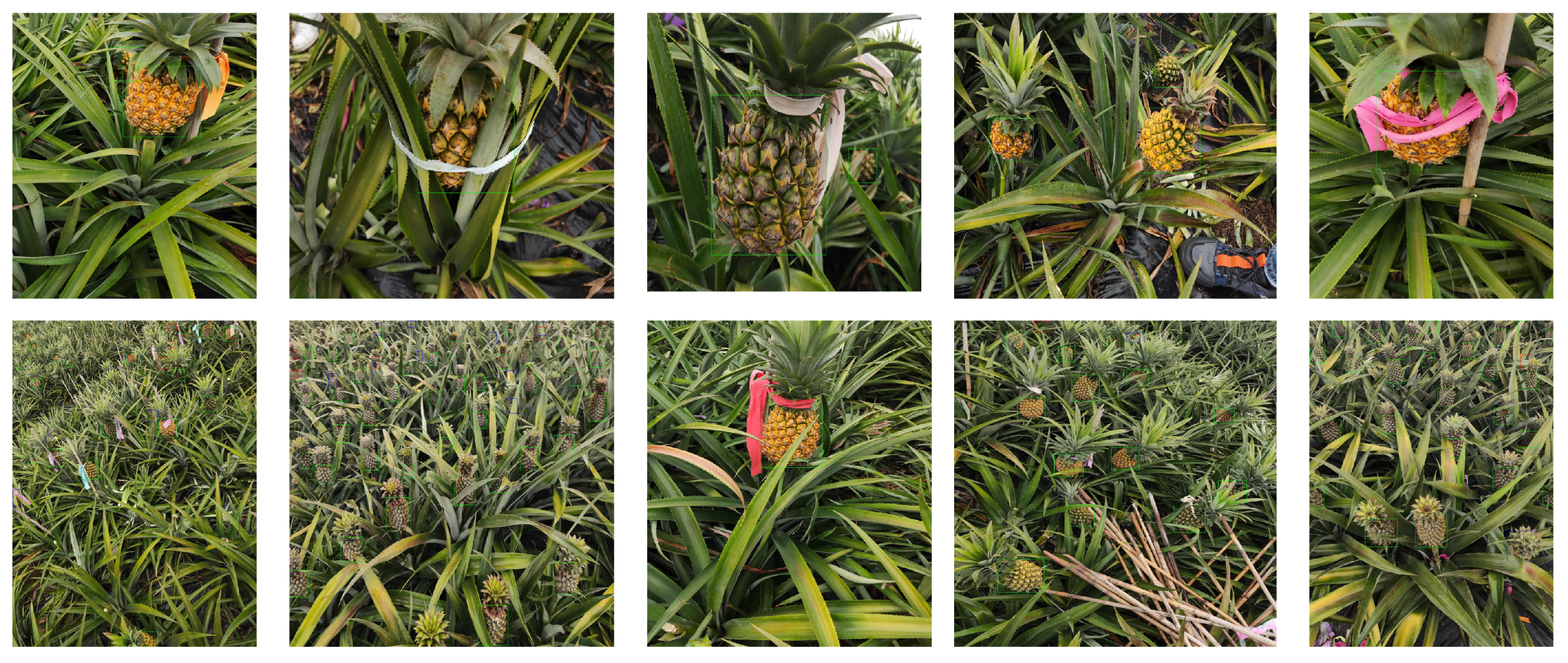
  • To enhance the flexibility and generalization of the visual model, we collected and constructed a dataset containing images of pineapples in various environments at the pineapple plantation base in Xuwen County, Zhanjiang City, Guangdong Province.
  • By replacing the main trunk network, introducing the lightweight GSConv module, and incorporating the decoupled head structure, improvements were made to the YOLOv7-tiny model, enhancing its detection accuracy and efficiency.
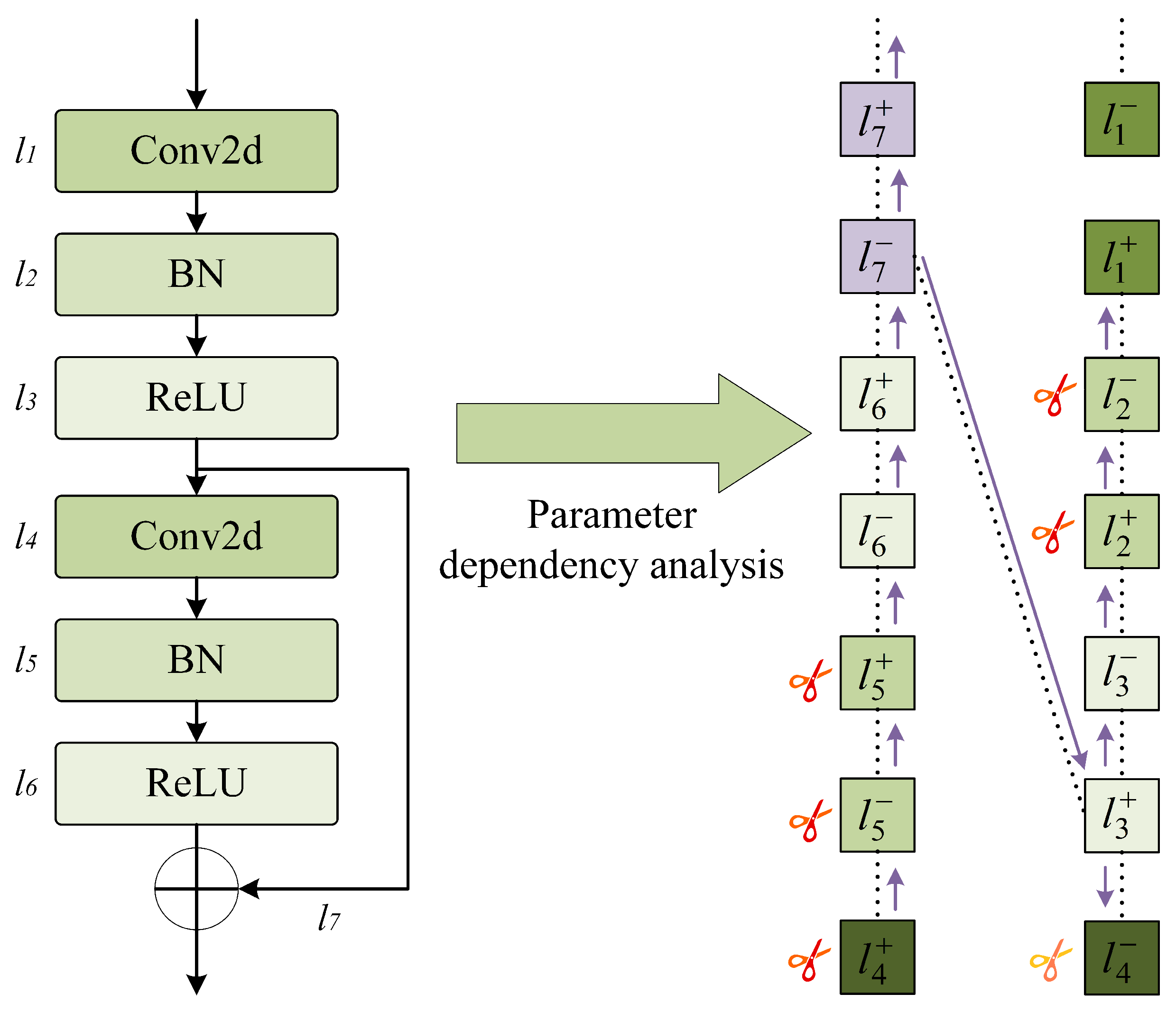
  • By applying the group-level pruning method based on the analysis of the dependency graph, the model was pruned. This effectively reduced the model’s complexity, maintained detection accuracy, and improved the model’s deployment efficiency on resource-constrained devices.
The rest of this paper is organized as follows. Section 2 introduces the construction of the dataset materials and the specific methods for the improvement of the visual network. Section 3 presents five comparative experiments that verify the improved network from different perspectives. Section 4 is the conclusion of this paper.

2. Materials and Methods

2.1. Building the Pineapple Dataset

In this research, we constructed a pineapple image dataset, to support and validate our object detection model. The image collection was carried out at a pineapple plantation in Xuwen County, Zhanjiang City, Guangdong Province. During the photography process, we were cognizant of the potential issues that class imbalance could pose for subsequent model training. To address this, we adopted various shooting strategies: selecting a range of shooting angles and capturing images at different times throughout the day, to ensure that the images comprehensively covered the various lighting conditions and occlusion scenarios that pineapples might encounter in their natural growth environment. This collection method enhanced the model’s generalization capability in the face of different environmental conditions. Ultimately, we successfully collected approximately 1100 high-resolution RGB pineapple images. To further enhance the effectiveness of model training and the accuracy of validation, we utilized the labeling dataset annotation software to annotate the target areas. There was only one target category annotated, named “pineapple”. Figure 1 shows the pineapple under different occlusion and lighting conditions. The collected images were then divided into training, validation, and test sets at a ratio of 70%, 20%, and 10%, respectively. This division ensured that the model could learn thoroughly during the training process and that its performance could be accurately evaluated during the validation and testing phases.

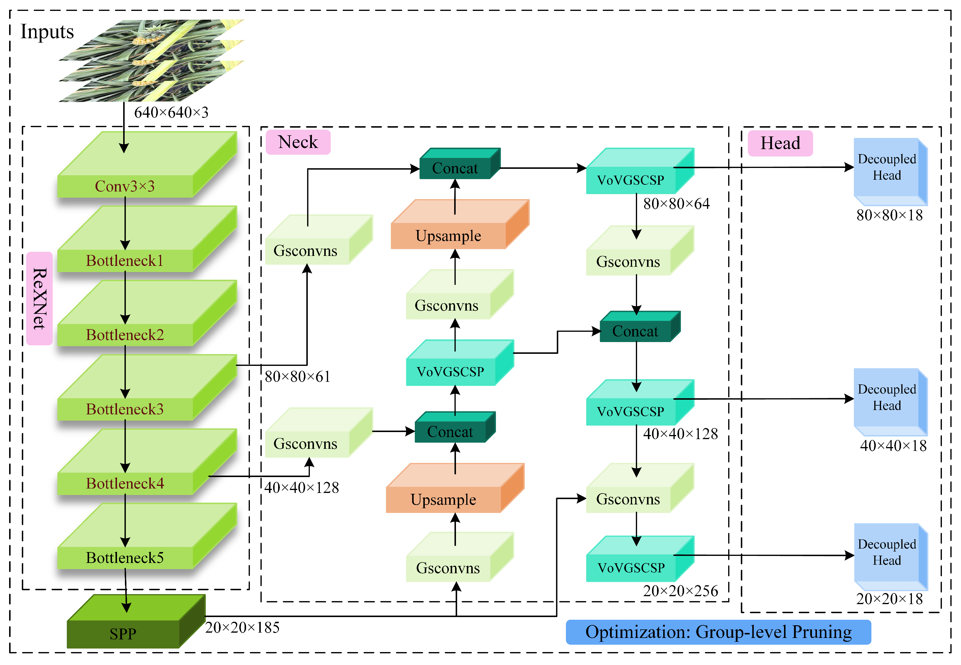
2.2. Improved YOLOv7-Tiny Network Framework

The network proposed in this paper, RGDP-YOLOv7-tiny, is an evolution of the traditional YOLO series, meticulously crafted to address the complexities of large-scale pineapple cultivation environments. It is composed of three integral sub-networks: a backbone network, a neck network, and a detection network. The backbone network, at the heart of the model, is a lightweight ReXNet designed to efficiently extract features from input data while reducing spatial dimensions and computational load. ReXNet incorporates depthwise separable convolutions and inverted residual structures, alongside a channel-wise progressive shrinking strategy, enhancing feature representation and minimizing computational overhead. Building upon the backbone’s output, the neck network integrates the innovative GSConv module. This module employs a unique channel-shuffling operation, to improve feature fusion across different channels, thereby augmenting the model’s ability to capture nuanced pineapple features amidst varying lighting and weather conditions, as well as the occlusion factors present in the dataset. Transitioning to the detection network, we replaced the original YOLOv7-tiny detection head with a decoupled head structure. This design separates the classification and localization tasks, allowing for a focused enhancement of the model’s convergence speed and detection accuracy. Each task now targets specific features, which is instrumental in improving the overall precision of the model.
Finally, to compress and optimize the model further, we employ sparse training, to guide the model in discerning dispensable parameters from crucial ones. Subsequently, a group-level pruning method, informed by a dependency graph analysis, is applied, to prune the less important parameters. This structured approach effectively reduces the model’s complexity without compromising its performance, aligning with the objectives of lightweight improvement work that begins with refining these three sub-networks. The structure of the RGDP-YOLOv7-tiny network is shown in Figure 2.

2.2.1. YOLOv7-Tiny Network Framework

YOLOv7-tiny is a lightweight version of the YOLOv7 algorithm [22,23,24]. It aims to maintain high detection accuracy while reducing the complexity of the model and resource consumption during runtime, making it more suitable for deployment in environments with limited resources.
Compared to the overall network architecture of YOLOv7, YOLOv7-tiny has reduced the stacking of convolutional blocks in both the ELAN layer and the SPPCSP layer, which decreases the model’s parameter count and computational complexity. In the neck network part, the multi-scale feature fusion method is retained. Through the feature pyramid fusion module and the feature pyramid alignment module, feature maps of different levels are interwoven, to better utilize the information from multi-level features. In the detection head part, standard convolution (SC) is used instead of RepConv, to further reduce the model’s parameter count. In the activation function part, LeakyReLU is chosen, to minimize computational expenses [25].
Despite its advantages in lightness and detection speed, YOLOv7-tiny still has some shortcomings: the core of the ELAN layer is one or more aggregation modules that are responsible for effectively fusing the input feature maps, which typically include cross-layer and residual connections. While these connections effectively preserve the information of both low-level and high-level features, they also increase the complexity of the network and, to some extent, the computational load. This paper proposes the use of other lightweight modules for improvement and, on this basis, further compresses the model’s computational load through model pruning.

2.2.2. Trunk Replacement

Researchers Dongyoon Han et al. from the NAVER AI Lab proposed Rank Expansion Networks (ReXNet) as an improvement and refinement of the lightweight network structure based on MobileNet [26]. The Google research team created MobileNet [27], a deep neural network architecture, with the express purpose of implementing effective neural network models on embedded systems and mobile devices. It reduces computational load and model size by adopting depthwise separable convolutions (DSC) and inverted residual structures [28].
However, many types of deep networks, including MobileNet, currently exhibit varying degrees of layer bottleneck issues: the low rank of network inputs does not adequately represent high-rank spaces. That is, if the resulting dimensions are relatively high when high-dimensional information is transformed into low-dimensional information then the loss of information is minimal. Conversely, if the resulting dimensions are relatively low, the loss of information is significant. After passing through the ReLU activation function, the loss of information is further exacerbated. The core concept of ReXNet is to incorporate the Swish activation function and to design additional expansion layers, to reduce the rank during each expansion, allowing the input dimensions to gradually approach the output dimensions. This unique channel dimension adjustment strategy not only maintains efficient computation but also significantly enhances the expressiveness of lightweight models in image-recognition tasks and classification tasks. It has not only advanced the design of lightweight models but has also paved new avenues and ideas for the optimization and exploration of network architectures.
With the specific structure described in Table 1, the ReXNet used in this paper is an improved version derived from the second-generation MobileNet architecture. The input image size has been changed from its original 214 × 214 dimensions to 640 × 640. The bottleneck structure, known as MB-bneck, is made up of 17 sequences in total. The squeeze-and-excitation attention mechanism module is integrated into the structures from sequences 5 through 17. Sequences 6, 12, and 17 function as the backbone’s three feature output layers, each of which is connected to the neck network. For these three output feature layers, the corresponding output channel numbers are 61, 128, and 185.

2.2.3. Neck Network Introduces the GSConv Lightweight Module

In convolutional neural networks, DSC refers to an operation where each input channel is convolved with a separate convolutional kernel. The structure of the DSC primarily consists of two parts: depthwise convolution and pointwise convolution. Compared to standard convolution, DSC avoids weight sharing, reducing the number of parameters and the computational cost, and it is often used in the design of lightweight neural networks. As shown in Figure 3, different convolutional structures are depicted.
The expressions of the parameter quantities P s c , P d s c and the calculation quantities S s c , S d s c of SC and DSC modules are as follows:
P s c = C i · K w · K h · C o
P d s c = C i · K w · K h + C o · C i
S s c = C i · K w · K h · C o · W · H
S d s c = C i · K w · K h · H · W + C o · C i · W · H
In the formulas, C i represents the number of input channels, while C o represents the number of output channels. K w and K h are the width and height of the convolutional kernel, respectively. W and H are the width and height of the feature map, respectively.
Since DSC lacks interaction between weights, the detection accuracy of networks built solely with DSC is typically lower. A balance between module weights and detection accuracy must be considered. Therefore, this paper replaces the SC and ELAN modules in YOLOv7-tiny with GSConvns and VoVGSCSP in the neck network [29], respectively. The specific structure is shown in Figure 4.
The GSConv structure depicted in the diagram is bifurcated into two pathways: the primary path first undergoes SC and DSC operations, followed by a concatenation with a secondary path that has no convolutional operations. Subsequently, a channel shuffle (CS) operation is employed, to permeate the information generated by SC into every segment of the DSC information, altering the channels to a specified dimension. CS is a channel mixing strategy that, by swapping local feature information across various channels, can fully integrate the information from DSC into the input of SC, thereby compensating for the lower detection accuracy inherent in DSC. Gsconvns represents a variant structure of Gsconv, where the original channel shuffle operation is substituted with a two-dimensional convolution followed by an activation function ReLU. This structure also blends the feature information emanating from the DSC output through two-dimensional convolution. VoVGSCSP strongly resembles GSConv, with the distinction that the channel shuffle operation is replaced by a standard convolution, and the DSC are supplanted by a GS bottleneck structure. The bottleneck layer structure, GS bottleneck, is composed precisely of two GSConv units and an SC module. These four configurations are applied to different convolutional layers within the neck network, augmenting the diversity of the network’s convolutional operations.

2.2.4. Detection Network Introduces Decouped Head

The detection head in a neural network is an essential component of object detection models, tasked with extracting and predicting the class and location of objects from feature maps. In the early versions of YOLO, the detection heads were typically coupled, meaning that the classification and localization tasks were performed simultaneously within the same network layer. Starting from YOLOv2, the series introduced the anchor box mechanism, which uses a predefined set of bounding boxes to match objects of various sizes. Following YOLOv3, the concept of multi-scale detection was introduced [30], which involves making predictions on feature maps at different layers, to detect objects at various scales. This paper retains the anchor box mechanism and multi-scale detection from the YOLO series and replaces the original coupled head structure with a decoupled head structure [31]. The decoupled head is based on the core idea of separating the classification and localization tasks in object detection. This structural change allows each task to focus on its specific features, thereby improving the model’s convergence rate and effectively reducing the number of parameters and computational complexity, thus providing enhanced performance in object-detection tasks. The structure of the decoupled head is illustrated in Figure 5. The numerical values of 256, 128, and 64 in the figure correspond to the number of output channels for the three stages of the neck network, respectively. Cls, Reg, and IoU represent the classification, location, and object score, respectively.

2.3. Model Compression

2.3.1. Model Pruning

Model pruning is a deep learning model optimization technique, primarily aimed at reducing the complexity of models and enhancing efficiency. By analyzing the weights in a neural network, pruning technology identifies and removes weights that have a minimal impact on the model’s output, thereby reducing the number of model parameters and computational requirements. This simplification can significantly decrease the model’s inference time, reducing latency. Additionally, pruning can reduce the model’s memory footprint, which helps to decrease the frequency of memory access and data exchange on devices, further lowering power consumption and extending the usage time and battery life of devices. At the same time, a smaller model size is also beneficial for deployment on mobile devices or embedded systems, reducing deployment costs and time.
The main pruning techniques nowadays are channel pruning, layer pruning, and unstructured pruning. Channel pruning reduces the width of the network by removing entire channels from convolutional layers, thereby reducing the model’s parameter count and computational complexity. However, this may affect the expressiveness of the features. Layer pruning involves removing entire convolutional layers from the network, which can significantly reduce the model’s depth, but may also lead to the loss of more feature information, affecting the model’s learning ability. Unstructured pruning is carried out at the weight level, without following the inherent structure of the network. This flexibility allows it to achieve a higher compression ratio without sacrificing network performance, but it may require special optimization strategies to deal with sparsity issues.
This paper utilizes group-level pruning as the model pruning method [32]. This structured pruning technique is applicable to various network architectures. It constructs a dependency graph to identify and model the structural interdependencies among layers within a neural network, and it groups the structured parameters within the network. Subsequently, parameters with low importance scores, as determined by subsequent sparse training, are pruned. This approach aims to reduce the model’s size and expedite the inference process.
The dependency graph is the core of the group-level pruning algorithm. Here is an explanation of the dependency graph: Due to the structural coupling relationships between layers within the same and different layers of a neural network, when one layer is pruned, another layer will also undergo corresponding changes. To achieve structured pruning, we need to analyze the interdependencies of layers, to group parameters: for example, a parameter group L = { l 1 , l 1 + , l 2 , l 2 + , , l n , l n + } , where each l refers to a parameterized layer, including convolutional (Conv2d) layers, batch normalization (BN) layers, and activation function layers, or a non-parameterized operation, such as residual addition. The positive and negative superscripts of l represent the outputs and inputs of the layers, respectively.
By focusing on the dependency relationships between layer inputs and outputs, a layer dependency model is constructed, as shown in Equation (5) for the dependency expression:
l 1 , l 1 + l 2 , l 2 + l n , l n +
The equation includes two types of layer dependencies: inter-layer dependency l i + , l j and intra-layer dependency l i , l i + . Inter-layer dependency refers to the direct association between adjacent layers in the network, where the output features of one layer serve directly as the input to the next layer, creating an end-to-end connection. Intra-layer dependency refers to the association between the inputs and outputs within a single layer. As shown in Figure 6, the parameter dependency analysis of two standard convolution modules with residual links is performed. The batch normalization layer is l 2 or l 5 , and their respective input and output are a pair of intra-layer dependencies and are coupled. However, the inputs and outputs of layer l 4 are not dependent on each other and are independent, yet we can still group them into the same parameter group and prune them with different pruning layouts, to achieve consistent cross-layer pruning. This enhances the efficiency of pruning and the accuracy of model compression.

2.3.2. Sparse Training

During the process of group-level pruning, batches of parameters are deleted simultaneously. To ensure the effectiveness of pruning, it is necessary to confirm that the deleted parameters are collectively unimportant, meaning their contribution to the network’s performance can be disregarded. If the group of parameters includes those that are crucial for the network’s predictive ability, removing them may lead to a significant degradation in network performance. In such cases, a strategy of sparse training is required to identify these parameters, allowing them to be safely removed during the pruning process.
This paper introduces a regularization term H g , k for the weight parameter group g = { w 1 , w 2 , , w g } with K dimensions that can be pruned. The purpose is to motivate the model to learn which parameters in the group g are expendable for pruning. The specific formulation is as follows:
H g , k = k = 1 K γ k · Q g , k
Q g , k = w g w [ k ] 2 2
γ k = 2 α Q g max Q g , k / Q g max Q g min
In Equation (6), y is a scaling factor that controls the sparsity strength of the k-th prunable dimension, while Q g , k denotes the importance score of the parameter w in the k-th prunable dimension within the parameter group g.
In Equation (7), w [ k ] represents the k-th parameter submatrix within the parameter group g, where w refers to the weight parameters of the neural network and k refers to a specific slice of the parameter matrix—that is, a subset selected from the entire parameter matrix. During group-level pruning, this slicing operation allows the algorithm to focus on the submatrix within the current parameters, thereby enabling independent analysis of each parameter group.
In Equation (8), α is a hyperparameter that controls the range of sparsity intensity, while Q max and Q min denote the maximum and minimum importance scores, respectively, within the parameter group g, which are used to determine the strength of sparsity.
Utilizing the sparse training algorithm described, we can identify k sets of parameters with varying levels of sparsity. We then select the set with the minimal L2 norm, which has the least detrimental effect on model performance, for group-level pruning of the network structure.

2.4. Model Evaluation Metrics

To evaluate the performance and complexity of the model, this study chose several metrics commonly used in object detection. These include precision, recall, the comprehensive evaluation metric F 1 , average precision ( A P ), mean average precision ( m A P ), the count of parameters (Params), the computational load, in terms of floating point operations (FLOPs), and the size of the model. The expressions for calculating the first five metrics are as follows:
P = T P T P + F P
R = T P T P + F N
F 1 = 2 P R P + R
A P = 0 1 P R d R
m A P = 1 C i = 0 c A P i
Equation (9) and Equation (10) represent precision and recall, respectively. In these equations, T P indicates true positives, where the actual class of the sample is positive and the prediction is also positive; TN indicates true negatives, where the actual class is negative and the prediction is negative; F P indicates false positives, where the actual class is negative but the prediction is positive; F N indicates false negatives, where the actual class is positive but the prediction is negative. Precision describes the proportion of true positives among the positives predicted by a binary classifier, while recall describes the proportion of actual positives that have been identified.
Equation (11) is the harmonic mean of precision and recall, known as the F1 score. Its value ranges from 0 to 1, with a value closer to 1 indicating better model performance. In practical applications, depending on the specific needs of the problem, we may focus more on either precision or recall, but the F1 score provides a measurement that takes both into account.
Equation (12) measures the performance of detection for a particular class, which can be understood as having recall on the horizontal axis and precision on the vertical axis of a coordinate system; the area where the curve intersects with both axes represents the average precision. The larger the intersecting area, the higher the A P value. Equation (13) calculates mean average precision, which assesses the overall effectiveness of detection across all classes.
The latter three metrics assess the complexity of the model. FLOPs refers to the number of floating-point operations per second, reflecting the amount of computational resources required to execute a neural network model. The number of parameters refers to the total count of learnable parameters within the neural network model, typically including weights and biases. Model size refers to the file size of the model, which affects the deployment efficiency of the model. Smaller models are easier to deploy on devices with limited resources, while larger models require longer transmission times and more bandwidth.

3. Experiments and Analysis

For this paper, we conducted the following four types of experiments: comparative experiments between YOLOv7-tiny and different lightweight backbones; comparative experiments with different pruning methods; comparative experiments under a wide range of pruning ratios; and comparative experiments with different target-detection algorithms and their corresponding pineapple detection visualization. The comparative experiment of pruning methods in Section 3.2 of this article compared the impact of different pruning techniques on the performance of the YOLOv7-tiny model. The experimental results provided a basis for selecting the most effective pruning method. The comparative experiment of pruning multiples in Section 3.3 of this article was an exploration of the depth of the selected pruning technology, with the aim of finding the optimal pruning ratio and achieving the best balance between model complexity and performance. The experiments on different target-detection algorithms in Section 3.4 and Section 3.5 of this article expanded the research horizon. The purpose of this section is to show the competitiveness and practicality of RGDP-YOLOv7-tiny in target-detection tasks, especially in resource-constrained environments. Each experiment in this section was based on the results of the previous step, gradually deepened, and, finally, formed a complete research process. The environment configuration of this experiment is shown in Table 2. The batch size of the experiment was set to 16, the training epoch was set to 300, and the image resolution was selected as 640 × 640.

3.1. Lightweight Backbone Comparative Experiment

To explore the performance of different lightweight backbones on YOLOv7-tiny, for this section we conducted a comparative analysis of models optimized at various pruning ratios for each lightweight backbone. YOLOv7-tiny was selected as the base network, and its backbone network was replaced with GhostNet [33], GhostNetv2 [34], FasterNet [35], ReXNet, and MobileNetv3 [36], respectively. Each network was pruned at pruning ratios of 1.0, 2.0, and 2.5. Subsequently, the models were fine-tuned and their performance was compared. The experimental results are presented in Table 3.
The data from Table 3 indicates that at a pruning ratio of 1.0, which means no pruning was applied, the YOLOv7-tiny network with the FasterNet and MobileNetv3 backbones had lower [email protected] and F1 scores compared to the original YOLOv7-tiny. However, when using GhostNet, GhostNetv2, and ReXNet as the backbones, these metrics were approximately 1.5% higher than the original YOLOv7-tiny. It should be noted that the GhostNet series reduced the parameter count, computational load, and model size, whereas ReXNet saw a slight increase; when the pruning ratio was 2.0, the [email protected], precision, recall, and F1 scores of the GhostNet series experienced a significant decrease, which may be attributed to excessive pruning, causing the model to lose information that was critical for classification and localization tasks. In contrast, ReXNet showed better anti-pruning performance, with its [email protected] and F1 scores increased by 0.9% and 0.6%, respectively, compared to the unpruned state. Compared to the original YOLOv7-tiny at a pruning ratio of 2.0, these improvements were 1.5% and 0.7% higher, respectively; when the pruning ratio reached 2.5, ReXNet’s F1 score rose by 0.8% compared to the original YOLOv7-tiny, and although the [email protected] dropped by 0.3%, ReXNet still demonstrated its advantages at this pruning level. Compared to its unpruned state, its parameter count, computational load, and model size were reduced by 39.4%, 39.2%, and 40.1%, respectively. This shows that ReXNet is more robust in structure and can better maintain its performance after pruning.

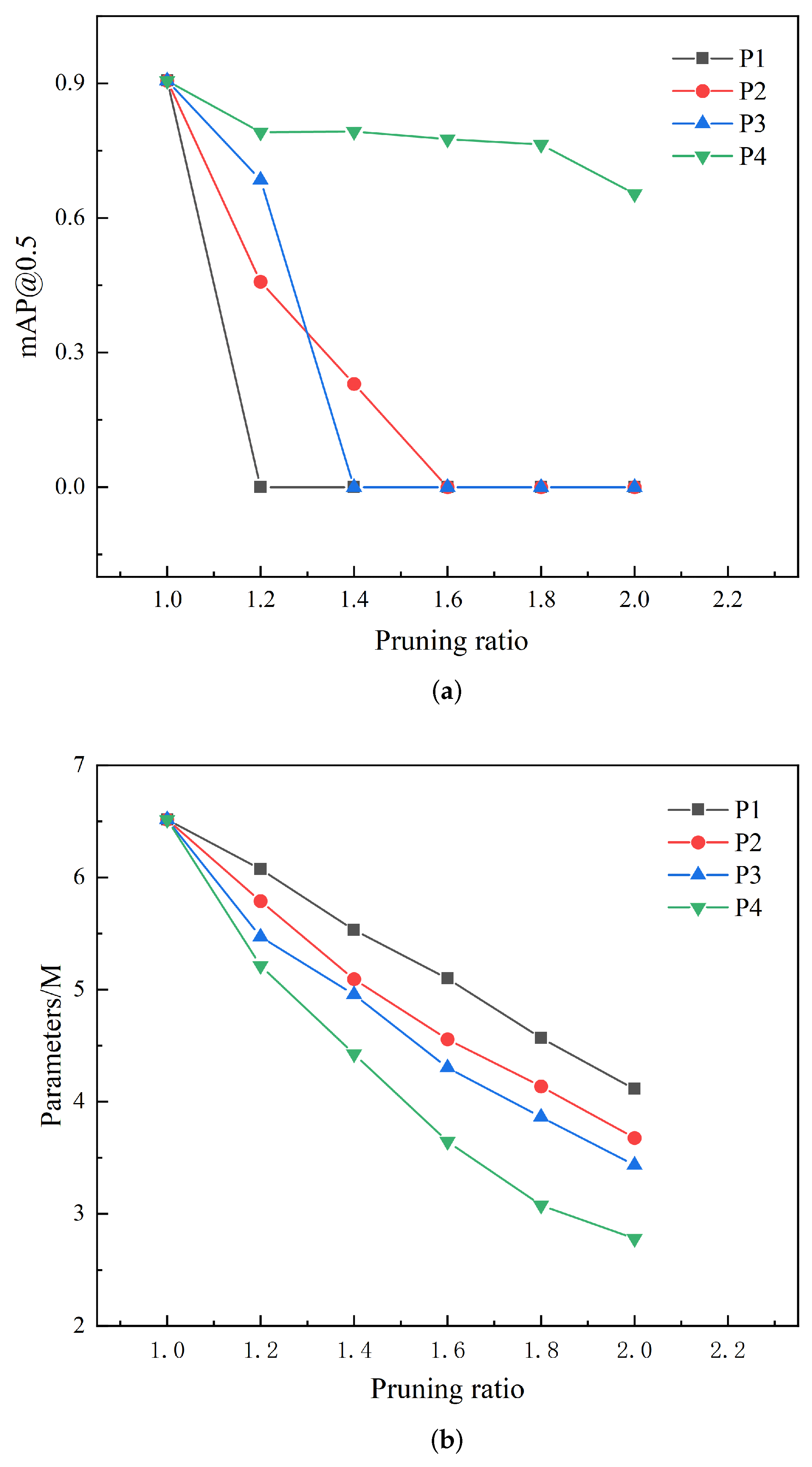
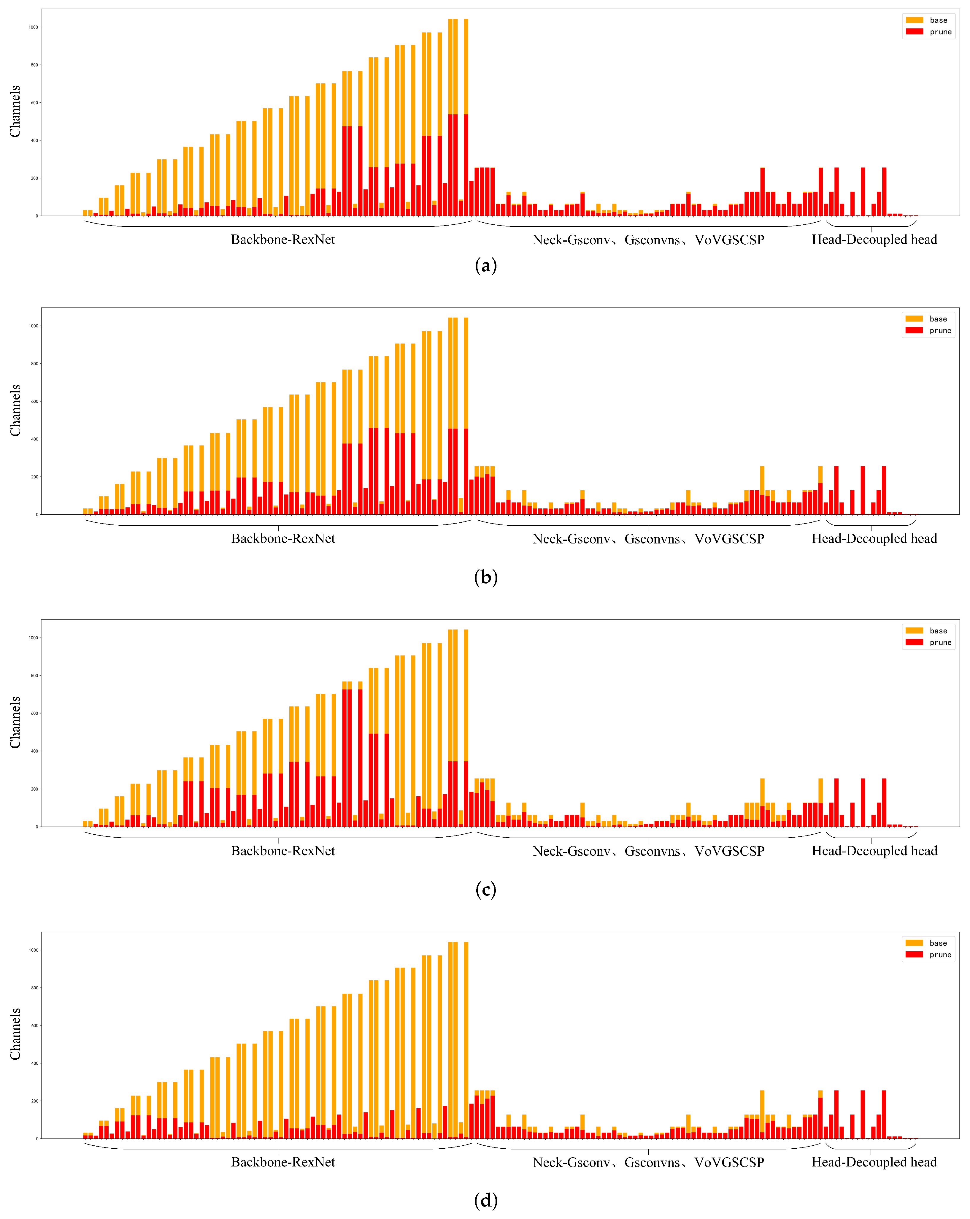
3.2. The Impact of Different Pruning Methods on Model Performance

To verify the advantages of the pruning methods adopted in this paper, various pruning techniques were applied to the network structure model depicted in Figure 2, followed by subsequent fine-tuning, to further optimize model performance. The specific pruning methods used included a filter pruning method based on the L1 norm (P1), a pruning method that evaluates the importance of neurons through the Taylor expansion of the loss function [37] (P2), a pruning method that assesses network weights based on the second-order derivatives of the objective function [38] (P3), and the group-level pruning method proposed in this paper (P4). The experimental results are shown in Table 4.
According to the comparative experimental results in Table 4, it can be observed that the group-level pruning method achieved the highest levels in key performance indicators, such as [email protected], F1 score, precision, and recall. This indicates that during the pruning process, the group-level pruning method effectively preserved parameters that were crucial for the network’s predictive performance, avoiding performance loss due to excessive pruning. Furthermore, from the perspective of model complexity, the group-level pruning method also showed a significant advantage in reducing the number of parameters, the computational load, and the model size. Compared to other pruning methods, it achieved the lowest model complexity, demonstrating greater efficiency in identifying and removing parameters that contribute less to model performance.
In summary, the group-level pruning method not only showed outstanding performance in improving model capabilities but also had a significant advantage in reducing model complexity. To delve deeper into the performance of the group-level pruning method, we analyzed the decline in [email protected] and parameter count as the pruning ratio increased during the pruning process, as illustrated in Figure 7, as well as the channel comparison chart for different pruning methods at a pruning ratio of 2.0, as shown in Figure 8. Through this visualization, we could more directly perceive the group-level pruning method’s capacity to balance model efficiency with the maintenance of predictive accuracy.
Figure 7a represents the curve of [email protected] as the pruning ratio increased. It can be observed that for pruning methods P1, P2, and P3, the [email protected] dropped to 0 when the pruning ratio reached 1.5. In contrast, method P4 maintained the [email protected] of around 80.0%. As the pruning ratio further increased to 2.0, the [email protected] of P4 could still be sustained at approximately 65.0%. This indicates that under the same pruning ratio, the model pruned by P4 had more potential to recover to the initial model’s accuracy after fine-tuning compared to the other pruning methods. At different pruning ratios, the impact of P4 pruning on model accuracy was relatively smaller, implying that more significant compression effects can be achieved at a higher pruning ratio. Figure 7b reveals how the model’s parameter count changed with the increase in pruning ratio, showing that compared to the other pruning methods, P4 pruning achieved the greatest degree of parameter reduction at any pruning ratio. Integrating these observations, we can conclude that the group-level pruning method used in this paper can maximize model compression at a higher pruning ratio while maintaining model performance.
As illustrated in Figure 8, the vertical axis represents the number of channels and the horizontal axis refers to the detailed convolutional operations within the three main network layers. The term “Base” denotes the model before pruning, while “Prune” indicates the model at a pruning ratio of 2.0. Among the four pruning methods, there was no significant difference in the channel compression effect in the neck and detection networks. However, in the ReXNet backbone network section, regardless of the pruning method applied, the number of channels could be significantly reduced. Under the P1, P2, and P3 pruning methods, the maximum number of channels in the backbone could be compressed to below 600, 500, and 800, respectively. In contrast, under the P4 pruning method, the maximum number of channels in the backbone could be compressed to below 200, achieving a channel compression ratio of approximately 80%, which was more than 1.6 times higher than that of the other pruning methods. This further confirms the superior model compression efficiency of the group pruning approach.

3.3. The Impact of Different Pruning Ratios on Model Performance

From Figure 7a, it can be observed that the [email protected] for the P4 pruning method did not drop to zero as the pruning ratio increased, unlike the other pruning methods. For models that [email protected] reduced to zero, their performance could still be improved, to some extent, after subsequent fine-tuning. Therefore, we had reason to further explore the impact on model performance across a broader range of pruning multiples.
In the following experiment, group-level pruning was applied to the network structure model shown in Figure 2, and the pruning ratio was gradually increased in a stepwise manner. The initial pruning ratio was set at 2.0, and it was increased by 0.1 with each step, up to a maximum of 3.0. The final model was obtained through fine-tuning. Detailed experimental data can be found in Table 5.
Based on the data from Table 5, it is evident that before pruning, the completely replaced network model saw an increase of 1.5% in [email protected] and 1.1% in the F1 score over the ReXNet-YOLOv7-tiny model. The parameter count, computational load, and model size were reduced by 0.12 × 10 6 , 0.6 × 10 9 , and 0.01 MB, respectively. Within the pruning ratio range of 2.0 to 2.5, the model’s performance remained relatively stable after fine-tuning, with no significant fluctuations. Meanwhile, the complexity metrics of the model, including parameter count, computational load, and model size, continued to decline. However, when the pruning ratio increased beyond 2.6, the model’s performance metrics began to decline noticeably and the rate of decrease in the complexity metrics also slowed. This indicated that within the pruning ratio range of 2.0 to 2.5 an equilibrium had been achieved between model performance and complexity. Beyond this range, further pruning began to negatively affect model performance, and the effect of reducing model complexity also gradually diminished. Consequently, the network structure in Figure 2, after a 2.5-times pruning, represents the final improved pruned lightweight pineapple detection network model RGDP-YOLOv7-tiny obtained in this paper. When comparing this model with the YOLOv7-tiny after a 2.5-times pruning, as listed in Table 3, RGDP-YOLOv7-tiny achieved higher compression ratios of 4.6% in parameter count and 3.9% in model size, with a 0.1% reduction in computational load. In short, the improved model’s compression effect is more pronounced than the original YOLOv7-tiny.

3.4. Performance Comparison of Different Object-Detection Algorithms

To objectively validate the proposed pruned lightweight pineapple-detection algorithm, this experiment compared six object-detection algorithms: YOLOv5s, YOLOv7, YOLOv7-tiny, YOLOv8s, YOLOv8n, and RGDP-YOLOv7-tiny. The results are shown in Table 6. It can be observed that the RGDP-YOLOv7-tiny network had a parameter count of 2.27 M, a computational load of 4.5 × 10 9 , and a model size of 5.0 MB. These complexity metrics are lower than those of other networks in the YOLO series. At the same time, the YOLOv7 network, with its higher model complexity, achieved [email protected] and F1 scores of 90.0% and 88.0%, respectively, ranking first among all the compared networks. However, the RGDP-YOLOv7-tiny also performed well, reaching 87.9% and 87.4%. These results highlight that RGDP-YOLOv7-tiny can maintain a high level of pineapple detection accuracy even with relatively lower resource consumption. Specifically, RGDP-YOLOv7-tiny outperformed other YOLO series networks in terms of parameter count, computational load, and model size, which implies not only computational efficiency but also more convenient application in agricultural robots.

3.5. Pineapple Detection Visualization

This section employs the Grad-CAM heatmap visualization technique to illustrate the output of deep learning models [39]. The essence of this technology lies in leveraging the gradient information of the model’s predictions concerning the input image. The gradients indicate the degree to which each pixel in the input image contributes to the model’s output class score. By calculating these gradients and combining them with the model’s intermediate feature maps, Grad-CAM can generate a heatmap. The intensity of colors on this heatmap represents the significance of each area to the model’s predictive outcome, with highlighted areas indicating areas of greater focus. Specifically, the six object-detection algorithms listed in Table 6 were used to create heatmaps, as shown in Figure 9.
To evaluate the performance and generalization capability of the RGDP-YOLOv7-tiny network in detecting pineapples under various environmental conditions, for this section we tested multiple typical scenarios, including unobstructed, foliage-obstructed, uneven lighting, dim environments, and situations with front and backlighting. The collected field-planted pineapple images were used to generate heatmaps with the Grad-CAM technique, to visualize the model’s predicted focus areas. Observing Figure 9, under the soft morning light and unobstructed conditions, the highlighted areas of the YOLOv7 and RGDP-YOLOv7-tiny networks were more concentrated, while the other networks were more dispersed. Under the four different lighting conditions at noon, the highlighted areas of the YOLOv5s, YOLOv7, and RGDP-YOLOv7-tiny networks were larger, showing impressive adaptability to lighting conditions, among which, the highlighted areas of the RGDP-YOLOv7-tiny were more concentrated, indicating that the network maintained high recognition accuracy under complex lighting conditions. Under the foliage obstruction, the level of highlighted areas drawn by the six networks was relatively average and the recognition performance of each network did not differ much. Overall, the heatmaps drawn by the YOLOv7 network had the widest and most concentrated highlighted areas, while the RGDP-YOLOv7-tiny network also demonstrated detection accuracy and generalization capability comparable to YOLOv7 while maintaining a lower parameter volume. This indicates that the RGDP-YOLOv7-tiny network not only maintains high precision in detecting pineapples but also has excellent generalization ability, capable of adapting to a variable field environment.

3.6. Performance of RGDP-YOLOv7-Tiny in Complex Scenarios

For this section, we explored the performance of the RGDP-YOLOv7-tiny model under diverse environmental conditions, through experiments, with a particular focus on its ability to handle false positives and false negatives when identifying targets in complex scenes. Figure 10 shows the results of 10 test images predicted by the RGDP-YOLOv7-tiny model, where green boxes represent true positives, blue boxes indicate false negatives, and red boxes signify false positives. The network detected a total of 132 target boxes, including 107 true positives, 10 false negatives, and 15 false positives. The green boxes predominantly appear in areas with abundant target features, while the blue and red boxes are mainly found in areas with fewer target features—that is, when the distance between the shooter and the target was farther then the resolution of the target object was reduced, leading to increased difficulty in feature extraction, which may be the main reason for missed and false detection. Considering that pineapple-harvesting robots mainly target objects at closer ranges, this network can meet the work requirements of pineapple-harvesting robots in practical applications. However, there is still room for improvement in the performance of long-distance targets. We will continue to explore model optimization strategies to enhance its robustness in different distances and complex environments, ensuring its efficiency and accuracy in actual harvesting operations.

4. Conclusions and Future Works

This paper addressed the application requirements of agricultural robots in large-scale planting environments by proposing an improved object detection model, RGDP-YOLOv7-tiny, designed to accommodate robotic platforms with limited computational resources. The model employs ReXNet as the backbone network, integrates GSConv into the neck network, and introduces a decoupled head in the detection network, ultimately achieving model compression through sparse training and group-level pruning optimization. Our experimental results demonstrated that, although the model’s complexity slightly increased before pruning and optimization, there was a 3.0% improvement in [email protected] and a 2.2% improvement in the F1 score, indicating that the model had greater potential for further compression in subsequent pruning processes. After pruning, the RGDP-YOLOv7-tiny model outperformed the original YOLOv7-tiny, with Params, FLOPs, and model size reduced from 6.01, 13.2 × 10 9 , and 12.3 MB to 2.27, 4.5 × 10 9 , and 5.0 MB, respectively, representing decreases of 37.8%, 34.1%, and 40.7%. Additionally, the [email protected] and F1 scores of RGDP-YOLOv7-tiny also improved by 0.8% and 1.3%, reaching 87.9% and 87.4%, respectively. Despite the significant reduction in size, the [email protected] and F1 scores of RGDP-YOLOv7-tiny remained higher than most of the YOLO series object-detection algorithms. The final heatmap visualization comparison also proved that the model maintains decent generalization performance across different pineapple cultivation environments, providing effective visual detection technology for pineapple agriculture robots. However, different pruning methods and lightweight modules exhibited varying adaptability to convolutional neural networks. In our future research, we plan to explore the adaptability between the various pruning methods and lightweight modules, aiming to further enhance the model’s performance under resource-constrained conditions. Additionally, we recognize that the model may have limitations when generalized to a variety of agricultural scenarios, while target-detection tasks are ubiquitous in the agricultural field. Therefore, we can leverage transfer learning technology and make appropriate adjustments and optimizations to extend the framework to broader applications, including the detection of other crop targets, crop disease detection, and weed identification. We believe that, through further research and development, exploring these possibilities in our future work will promote the development of smart agriculture and contribute to the advancement of agricultural robot vision technology.

Author Contributions

Conceptualization, J.L. (Jiehao Li); formal analysis, C.L. and Q.L.; funding acquisition, J.L. (Jiehao Li); investigation, Y.L., C.L. and J.L. (Jiahuan Lu); methodology, J.L. (Jiehao Li), Y.L. and C.L.; project administration, J.L. (Jiehao Li); resources, J.L. (Jiahuan Lu); software, Q.L.; supervision, J.L. (Jiahuan Lu); validation, Q.L.; visualization, Y.L. and C.L.; writing—original draft, J.L. (Jiehao Li) and Y.L.; writing—review and editing, J.L. (Jiehao Li). All authors have read and agreed to the published version of the manuscript.

Funding

This research was funded by 2024 Basic and Applied Research Project of Guangzhou Science and Technology Plan, grant number: 2024A04J4140 and State Key Laboratory of Robotics and Systems (HIT), grant number: SKLRS-2024-KF-08 and The APC was funded by Jiehao Li.

Data Availability Statement

The original contributions presented in the study are included in the article, further inquiries can be directed to the corresponding author.

Acknowledgments

This work was supported by the 2024 Basic and Applied Research Project of Guangzhou Science and Technology Plan under Grant 2024A04J4140, the State Key Laboratory of Robotics and Systems (HIT) under Grant SKLRS-2024-KF-08, and the Young Talent Support Project of Guangzhou Association for Science and Technology under Grant QT2024-006.

Conflicts of Interest

The authors declare no conflicts of interest. The funders had no role in the design of the study; in the collection, analyses, or interpretation of data; in the writing of the manuscript, or in the decision to publish the results.

References

  1. Liu, C.; Liu, Y. Current status of pineapple production and research in China. Guangdong Agric. Sci. 2010, 10, 65–68. [Google Scholar]
  2. Li, D.; Jing, M.; Dai, X.; Chen, Z.; Ma, C.; Chen, J. Current status of pineapple breeding, industrial development, and genetics in China. Euphytica 2022, 218, 85. [Google Scholar] [CrossRef]
  3. He, F.; Zhang, Q.; Deng, G.; Li, G.; Yan, B.; Pan, D.; Luo, X.; Li, J. Research Status and Development Trend of Key Technologies for Pineapple Harvesting Equipment: A Review. Agriculture 2024, 14, 975. [Google Scholar] [CrossRef]
  4. Shu, H.; Sun, W.; Xu, G.; Zhan, R.; Chang, S. The Situation and Challenges of Pineapple Industry in China. Agric. Sci. 2019, 10, 683. [Google Scholar] [CrossRef]
  5. Jiang, T.; Guo, A.; Cheng, X.; Zhang, D.; Jin, L. Structural design and analysis of pineapple automatic picking-collecting machine. Chin. J. Eng. Des. 2019, 26, 577–586. [Google Scholar]
  6. Li, J.; Dai, Y.; Su, X.; Wu, W. Efficient Dual-Branch Bottleneck Networks of Semantic Segmentation Based on CCD Camera. Remote Sens. 2022, 14, 3925. [Google Scholar] [CrossRef]
  7. Zhao, D.H.; Zhang, H.; Hou, J.X. Design of Fruit Picking Device Based on the Automatic Control Technology. Key Eng. Mater. 2014, 620, 471–477. [Google Scholar] [CrossRef]
  8. Pengcheng, B.; Jianxin, L.; Weiwei, C. Research on lightweight convolutional neural network technology. Comput. Eng. Appl. 2019, 16, 25–35. [Google Scholar]
  9. Li, J.; Li, J.; Zhao, X.; Su, X.; Wu, W. Lightweight detection networks for tea bud on complex agricultural environment via improved YOLO v4. Comput. Electron. Agric. 2023, 211, 107955. [Google Scholar] [CrossRef]
  10. Liu, X.; Wang, J.; Li, J. URTSegNet: A real-time segmentation network of unstructured road at night based on thermal infrared images for autonomous robot system. Control Eng. Pract. 2023, 137, 105560. [Google Scholar] [CrossRef]
  11. Li, B.; Ning, W.; Wang, M.; Li, L. In-field pineapple recognition based on monocular vision. Trans. Chin. Soc. Agric. Eng. 2010, 26, 345–349. [Google Scholar]
  12. Li, X. Design of automatic pineapple harvesting machine based on binocular machine vision. J. Anhui Agric. Sci. 2019, 47, 207–210. [Google Scholar]
  13. Yang, W.; Rui, Z.; ChenMing, W.; Meng, W.; XiuJie, W.; YongJin, L. A survey on deep-learning-based plant phenotype research in agriculture. Sci. Sin. Vitae 2019, 49, 698–716. [Google Scholar]
  14. Zheng, Y.; Li, G.; Li, Y. Survey of application of deep learning in image recognition. Comput. Eng. Appl. 2019, 55, 20–36. [Google Scholar]
  15. Sun, D.; Zhang, K.; Zhong, H.; Xie, J.; Xue, X.; Yan, M.; Wu, W.; Li, J. Efficient Tobacco Pest Detection in Complex Environments Using an Enhanced YOLOv8 Model. Agriculture 2024, 14, 353. [Google Scholar] [CrossRef]
  16. Chunman, Y.; Cheng, W. Development and application of convolutional neural network model. J. Front. Comput. Sci. Technol. 2021, 15, 27. [Google Scholar]
  17. Xu, L.; Huang, H.; Ding, W.; Fan, Y. Detection of small fruit target based on improved DenseNet. J. Zhejiang Univ. (Eng. Sci.) 2021, 55, 377–385. [Google Scholar]
  18. Pengfei, Z.; Mengbo, Q.; Kaiqi, Z.; Yijie, S.; Haoyu, W. Improvement of Sweet Pepper Fruit Detection in YOLOv7-Tiny Farming Environment. Comput. Eng. Appl. 2023, 59, 329–340. [Google Scholar]
  19. Liang, X.; Pang, Q.; Yang, Y.; Wen, C.; Li, Y.; Huang, W.; Zhang, C.; Zhao, C. Online detection of tomato defects based on YOLOv4 model pruning. Trans. Chin. Soc. Agric. Eng 2022, 6, 283–292. [Google Scholar]
  20. Yinghui, K.; Chengcheng, Z.; LinLin, C. Flower recognition in complex background and model pruning based on MobileNets. Sci. Technol. Eng. 2018, 18, 84–88. [Google Scholar]
  21. Li, J.Y.; Zhao, Y.K.; Xue, Z.E.; Cai, Z.; Li, Q. A survey of model compression for deep neural networks. Chin. J. Eng. 2019, 41, 1229–1239. [Google Scholar] [CrossRef]
  22. Wang, C.Y.; Bochkovskiy, A.; Liao, H.Y.M. YOLOv7: Trainable bag-of-freebies sets new state-of-the-art for real-time object detectors. In Proceedings of the IEEE/CVF Conference on Computer Vision and Pattern Recognition, Vancouver, BC, Canada, 18–22 June 2023; pp. 7464–7475. [Google Scholar]
  23. Zhou, J.; Zhang, Y.; Wang, J. RDE-YOLOv7: An improved model based on YOLOv7 for better performance in detecting dragon fruits. Agronomy 2023, 13, 1042. [Google Scholar] [CrossRef]
  24. Yang, H.; Liu, Y.; Wang, S.; Qu, H.; Li, N.; Wu, J.; Yan, Y.; Zhang, H.; Wang, J.; Qiu, J. Improved apple fruit target recognition method based on YOLOv7 model. Agriculture 2023, 13, 1278. [Google Scholar] [CrossRef]
  25. Xu, J.; Li, Z.; Du, B.; Zhang, M.; Liu, J. Reluplex made more practical: Leaky ReLU. In Proceedings of the 2020 IEEE Symposium on Computers and Communications (ISCC), Rennes, France, 7–10 July 2020; IEEE: Piscataway, NJ, USA, 2020; pp. 1–7. [Google Scholar]
  26. Han, D.; Yun, S.; Heo, B.; Yoo, Y. Rethinking channel dimensions for efficient model design. In Proceedings of the IEEE/CVF Conference on Computer Vision and Pattern Recognition, Nashville, TN, USA, 19–25 June 2021; pp. 732–741. [Google Scholar]
  27. Bi, C.; Wang, J.; Duan, Y.; Fu, B.; Kang, J.R.; Shi, Y. MobileNet based apple leaf diseases identification. Mob. Netw. Appl. 2022, 27, 172–180. [Google Scholar] [CrossRef]
  28. Sun, J.; Tan, W.; Wu, X.; Shen, J.; Lu, B.; Dai, C. Real-time recognition of sugar beet and weeds in complex backgrounds using multi-channel depth-wise separable convolution model. Trans. Chin. Soc. Agric. Eng. (Trans. CSAE) 2019, 35, 184–190. [Google Scholar]
  29. Zhao, X.; Song, Y. Improved Ship Detection with YOLOv8 Enhanced with MobileViT and GSConv. Electronics 2023, 12, 4666. [Google Scholar] [CrossRef]
  30. Lin, T.Y.; Dollár, P.; Girshick, R.; He, K.; Hariharan, B.; Belongie, S. Feature pyramid networks for object detection. In Proceedings of the IEEE Conference on Computer Vision and Pattern Recognition, Honolulu, HI, USA, 21–26 July 2017; pp. 2117–2125. [Google Scholar]
  31. Qiu, M.; Huang, L.; Tang, B.H. Bridge detection method for HSRRSIs based on YOLOv5 with a decoupled head. Int. J. Digit. Earth 2023, 16, 113–129. [Google Scholar] [CrossRef]
  32. Fang, G.; Ma, X.; Song, M.; Mi, M.B.; Wang, X. Depgraph: Towards any structural pruning. In Proceedings of the IEEE/CVF Conference on Computer Vision and Pattern Recognition, Vancouver, BC, Canada, 18–22 June 2023; pp. 16091–16101. [Google Scholar]
  33. Han, K.; Wang, Y.; Tian, Q.; Guo, J.; Xu, C.; Xu, C. Ghostnet: More features from cheap operations. In Proceedings of the IEEE/CVF Conference on Computer Vision and Pattern Recognition, Seattle, DC, USA, 14–19 June 2020; pp. 1580–1589. [Google Scholar]
  34. Tang, Y.; Han, K.; Guo, J.; Xu, C.; Xu, C.; Wang, Y. GhostNetv2: Enhance cheap operation with long-range attention. Adv. Neural Inf. Process. Syst. 2022, 35, 9969–9982. [Google Scholar]
  35. Chen, J.; Kao, S.h.; He, H.; Zhuo, W.; Wen, S.; Lee, C.H.; Chan, S.H.G. Run, Don’t walk: Chasing higher FLOPS for faster neural networks. In Proceedings of the IEEE/CVF Conference on Computer Vision and Pattern Recognition, Vancouver, BC, Canada, 18–22 June 2023; pp. 12021–12031. [Google Scholar]
  36. Howard, A.; Sandler, M.; Chu, G.; Chen, L.C.; Chen, B.; Tan, M.; Wang, W.; Zhu, Y.; Pang, R.; Vasudevan, V.; et al. Searching for mobilenetv3. In Proceedings of the IEEE/CVF International Conference on Computer Vision, Seoul, Republic of Korea, 27 October–2 November 2019; pp. 1314–1324. [Google Scholar]
  37. Molchanov, P.; Mallya, A.; Tyree, S.; Frosio, I.; Kautz, J. Importance estimation for neural network pruning. In Proceedings of the IEEE/CVF Conference on Computer Vision and Pattern Recognition, Long Beach, CA, USA, 15–20 June 2019; pp. 11264–11272. [Google Scholar]
  38. LeCun, Y.; Denker, J.; Solla, S. Optimal brain damage. Adv. Neural Inf. Process. Syst. 1989, 2, 598–605. [Google Scholar]
  39. Selvaraju, R.R.; Cogswell, M.; Das, A.; Vedantam, R.; Parikh, D.; Batra, D. Grad-cam: Visual explanations from deep networks via gradient-based localization. In Proceedings of the IEEE International Conference on Computer Vision, Venice, Italy, 22–29 October 2017; pp. 618–626. [Google Scholar]
Figure 1. (a) Sunny morning (unobstructed). (b) Sunny morning (foliage obstruction). (c) Sunny noon (uneven light). (d) Sunny noon (sunlit). (e) Sunny noon (backlit). (f) Evening.
Remotesensing 16 02805 g001
Figure 2. Total network architecture diagram.
Remotesensing 16 02805 g002
Figure 3. (a) Standard convolution. (b) Depthwise separable convolution.
Remotesensing 16 02805 g003
Figure 4. The module structures of GSConv, GSConvns, VOVGSCSP, and GS bottleneck.
Remotesensing 16 02805 g004
Figure 5. Structure of decoupled head.
Remotesensing 16 02805 g005
Figure 6. Dependency graph analysis.
Remotesensing 16 02805 g006
Figure 7. (a) The curve of [email protected] with the incremental increase of pruning ratio. (b) The curve of the number of parameters with the incremental increase of pruning ratio.
Remotesensing 16 02805 g007
Figure 8. (a) P1 pruning. (b) P2 pruning. (c) P3 pruning. (d) P4 pruning.
Remotesensing 16 02805 g008
Figure 9. Heatmap visualization.
Remotesensing 16 02805 g009
Figure 10. Detection results of the RGDP-YOLOv7-tiny network.
Remotesensing 16 02805 g010
Table 1. The network structure of ReXNet.
SequentialInputOperatorOutputStride
1 640 2 × 3Conv 3 × 3322
2 320 2 × 32MB-bneck1161
3 320 2 × 16MB-bneck6272
4 160 2 × 27MB-bneck6381
5 160 2 × 38MB-bneck6502
6 80 2 × 50MB-bneck6611
7 80 2 × 61MB-bneck6722
8 40 2 × 72MB-bneck6841
9 40 2 × 84MB-bneck6951
10 40 2 × 95MB-bneck61061
11 40 2 × 106MB-bneck61171
12 40 2 × 117MB-bneck61281
13 40 2 × 128MB-bneck61402
14 20 2 × 140MB-bneck61511
15 20 2 × 151MB-bneck61621
16 20 2 × 162MB-bneck61741
17 20 2 × 174MB-bneck61851
18 20 2 × 185Conv 1 × 1, pool 7 × 712801
19 1 2 × 1280Fc10001
Table 2. Experimental configuration.
ConfigurationParameters
CPUI5-12600KF
GPUNVIDIA GeForce RTX 4060 Ti
Operating systemWindows 10
Accelerated environmentCUDA 12.1.0; CUDNN 8.9.4.25
LibraryPytorch 2.1.1; Torch-Pruning 1.3.6
Table 3. Comparison of pruning results of YOLOv7-tiny under different backbone networks.
ModelPruning Ratio[email protected] (%)Precision (%)Recall (%)F1 Score (%)Params (M)FLOPs ( 10 9 )Model Size (MB)
1.087.192.980.286.16.0113.212.3
YOLOv7-tiny2.088.093.381.787.13.06.56.3
2.586.889.781.785.52.375.25.0
1.088.493.181.987.14.297.59.0
GhostNet-YOLOv7-tiny2.080.090.371.880.01.763.73.9
2.579.089.071.679.41.43.03.2
1.089.795.282.388.34.597.99.6
GhostNetv2-YOLOv7-tiny2.080.489.073.280.31.93.84.2
2.580.288.874.380.91.53.13.4
1.085.589.779.184.15.6511.411.6
FasterNet-YOLOv7-tiny2.086.092.579.385.43.095.66.5
2.585.491.778.884.82.434.55.1
1.088.693.481.787.26.6412.013.7
ReXNet-YOLOv7-tiny2.089.594.881.787.83.096.06.6
2.586.592.880.786.32.574.75.5
1.085.993.577.684.84.486.79.3
MobileNetv3-YOLOv7-tiny2.082.589.076.282.11.863.34.0
2.583.394.773.983.01.722.63.8
Table 4. Comparison results of different pruning methods.
Pruning MethodsPruning Ratio[email protected] (%)Precision (%)Recall (%)F1 Score (%)Params (M)FLOPs ( 10 9 )Model Size (MB)
P12.074.287.564.574.34.115.78.7
P283.992.175.182.73.645.67.8
P376.988.267.876.73.435.67.4
P487.992.581.786.82.775.76.0
Table 5. Comparison results at different pruning ratios.
Pruning Ratio[email protected] (%)Precision (%)Recall (%)F1 Score (%)Params (M)FLOPs ( 10 9 )Model Size (MB)
1.090.191.685.388.36.5211.413.6
2.087.992.581.786.82.775.76.0
2.187.491.481.085.92.605.35.7
2.287.893.180.386.22.495.15.5
2.387.092.680.286.02.394.95.3
2.487.791.382.386.62.334.75.1
2.587.994.981.087.42.274.55.0
2.685.289.379.784.22.214.34.9
2.774.484.368.575.62.164.24.8
2.874.589.666.376.22.094.04.7
2.974.188.665.275.12.043.94.6
3.074.385.765.974.51.953.84.4
Table 6. Comparison of different object-detection algorithms.
Pruning Ratio[email protected] (%)Precision (%)Recall (%)F1 Score (%)Params (M)FLOPs ( 10 9 )Model Size (MB)
YOLOv5s85.891.577.083.67.0215.914.4
YOLOv790.093.283.388.037.20105.174.8
YOLOv7-tiny87.192.980.286.16.0113.212.3
YOLOv8n87.692.980.286.13.018.26.3
YOLOv8s87.290.481.185.511.1428.622.5
RGDP-YOLOv7-tiny87.994.981.087.42.274.55.0
Disclaimer/Publisher’s Note: The statements, opinions and data contained in all publications are solely those of the individual author(s) and contributor(s) and not of MDPI and/or the editor(s). MDPI and/or the editor(s) disclaim responsibility for any injury to people or property resulting from any ideas, methods, instructions or products referred to in the content.

