Article

Mitigation of Suppressive Interference in AMPC SAR Based on Digital Beamforming

College of Electronic Science and Technology, National University of Defense Technology, No. 109 Deya Road, Changsha 410073, China
*
Author to whom correspondence should be addressed.
Remote Sens. 2024, 16(15), 2812; https://doi.org/10.3390/rs16152812
Submission received: 24 June 2024 / Revised: 29 July 2024 / Accepted: 29 July 2024 / Published: 31 July 2024

Abstract

:
Multichannel Synthetic Aperture Radar (MC-SAR) systems, such as Azimuth Multi-Phase Centre (AMPC) SAR, provide an effective solution for achieving high-resolution wide-swath (HRWS) imaging by reducing the pulse repetition frequency (PRF) to increase the swath width. However, in an Electronic Countermeasures (ECM) environment, the image quality of multichannel SAR systems can be significantly degraded by electromagnetic interference. Previous research into interference and counter-interference techniques has predominantly focused on single-channel SAR systems, with relatively few studies addressing the specific challenges faced by MC-SAR systems. This paper uses the classical spatial filtering technique of adaptive digital beamforming (DBF). Considering the Doppler ambiguity present in the echoes, two schemes—Interference Reconstruction And Cancellation (IRC) and Channel Grouping Nulling (CGN)—are designed to effectively eliminate suppressive interference. The IRC method eliminates the effects of interference without losing spatial degrees of freedom, ensuring effective suppression of Doppler ambiguity in subsequent processing. This method shows significant advantages under conditions of strong Doppler ambiguity and low jammer-to-signal ratio. Conversely, the CGN method mitigates the effect of interference on multichannel imaging at the expense of degrees of freedom redundant to Doppler ambiguity suppression. It shows remarkable interference suppression performance under weak-Doppler-ambiguity conditions, allowing for better image recovery. Simulations performed on point and distributed targets have validated that the proposed methods can effectively remove interfering signals and achieve high-resolution wide-swath (HRWS) SAR images.

1. Introduction

Synthetic Aperture Radar (SAR) provides all-weather day and night remote sensing and surveillance capabilities and is playing an increasingly important role in both civil exploration and military applications [1,2,3,4,5]. As a broadband radar system, SAR is highly susceptible to strong interference. With the increasing complexity of the electromagnetic environment and the presence of various active electronic jammers [6,7], obtaining high-resolution images of targets under such conditions remains a focal point of current SAR research.
SAR interference is generally divided into two types, deceptive interference and suppressive interference, and this paper focuses on suppressive interference. In deceptive interference, the jammer usually modulates and retransmits the intercepted SAR signals to create a false target in the image to confuse the adversary [8,9,10,11]. Compared to deceptive interference, suppressive interference is simple in principle and easy to implement. The suppressive interference that affects Synthetic Aperture Radar (SAR) imaging relies primarily on the high power of the interference signal to mask the desired signals in time, frequency and space [12,13]. This results in the necessary information within the imaging area being lost in the interference signal, which can severely affect airborne and spaceborne SAR systems [14,15]. Although SAR achieves a high energy accumulation gain through two-dimensional matched filtering, thereby reducing the likelihood of interference to some extent, strong interference sources inevitably degrade the quality and usability of SAR images, subsequently affecting the radar’s ability to observe targets [16].
Increasingly, sensors are required to provide simultaneous high-resolution and wide-swath (HRWS) continuous mapping capabilities for modern spaceborne Earth observation missions. PRF selection in traditional single-channel SAR is constrained by both range and azimuth ambiguities. On the one hand, achieving high azimuth resolution requires increasing the PRF to avoid azimuth aliasing. On the other hand, increasing the swath width requires decreasing the PRF to avoid range ambiguity, making it challenging to achieve both high resolution and a wide swath simultaneously [17]. The inherent contradiction between high pulse repetition frequency (PRF) and swath width has been mitigated by multichannel Synthetic Aperture Radar (SAR), exemplified by azimuth multiple phase centre (AMPC) SAR [18,19,20,21,22,23]. These systems exploit the deterministic relationship between the Doppler frequency of the echoes and the squint angle of the target, together with multiple spatial degrees of freedom, to provide high-resolution wide-swath imaging. Such capabilities have been widely used in ground moving target indication (GMTI) and sea clutter suppression [24,25].
The abundance of spatial degrees of freedom in the AMPC SAR system not only addresses azimuth ambiguities, but also creates favourable conditions for interference suppression. In general, the basic idea behind interference suppression techniques is to identify a suitable region where the characteristic differences between useful echoes and interference can be exploited to apply interference mitigation strategies. The interference is then extracted and removed or directly filtered out with minimal impact on the target echoes. Interference mitigation techniques can be divided into three categories according to their processing methods: non-parametric methods, parametric methods and semi-parametric methods [26]. Interference can be effectively mitigated by the integration of interference suppression techniques in the time domain, the frequency domain and the spatial domain, among other operational domains.
To the best of our knowledge, previous studies have mainly focused on single-channel SAR imaging systems, with relatively less attention paid to interference research in multichannel SAR systems. Interference in multichannel modes poses new challenges for multichannel SAR imaging while, at the same time, opening up a new field of research in multichannel SAR anti-interference technologies. On the one hand, the analysis of multichannel interference is different from that of single-channel systems, and, on the other hand, multichannel SAR offers numerous advantages over single-channel systems. By increasing the number of receiving channels, the redundancy in the received echo information is increased, which, together with the increased system degrees of freedom, enables the use of multichannel echo data for interference cancellation and anti-interference processing in both spatial and temporal domains. The basic concept is to use array beamforming techniques to direct the nulls of the antenna pattern towards the sources of interference. In recent years, appropriate anti-interference algorithms for multichannel SAR, including interference localisation methods and interference suppression techniques, have received considerable attention. Yu et al. [27] proposed a single spurious localisation algorithm based on the conjugate cross-correlation of two-channel SAR signals which strictly requires the spurious signal energy to be significantly larger than the true target signal. In addition, the sensitivity to the initial iteration values greatly affects the localisation accuracy. Lin et al. [28] used the direction of arrival (DOA) method to determine the angle between the SAR and the jammer. References [29,30] proposed slow-time and fast-time space–time adaptive processing (STAP) techniques for interference suppression, respectively, using spatial sampling information provided by multiple channels and the correlated pulse sequences obtained within the synthetic aperture time to design space–time adaptive filters for active interference suppression. Bollian et al. proposed the use of digital beamforming techniques in a 32-channel EcoSAR system [31]. Inspired by the phase centre antenna interference suppression technique [32], reference [33] proposed a dual-channel cancellation method to suppress interference signals. This method uses the phase relationship between the echo signals received from different channels to cancel the signals from stationary jammers. The method is easy to implement and has low computational complexity. However, the above interference methods require the signals to have a clear spectrum to ensure that single channel echoes can be imaged without Doppler ambiguity caused by undersampling, which directly leads to the loss of HRWS capability in multichannel SAR. Reference [34] proposed a Joint Azimuth Multichannel Cancellation (JAMC) anti-interference scheme for HRWS SAR systems by designing a joint cancellation filter on the basis of the phase differences of the interference signals received by different SAR channels to eliminate interference. Reference [35] adopted a sparse regularisation method in the image domain to protect the true echoes of the SAR system and mitigate NBI by solving the low-rank recovery problem of NBI. Current research on interference suppression for high-resolution wide-swath (HRWS) Synthetic Aperture Radar (SAR) systems focuses primarily on the traditional slow time domain echo model. The spatial angle advantages inherent in multichannel SAR systems have not been thoroughly analysed. Furthermore, there remains a lack of comprehensive studies investigating the effects of different interference patterns and developing appropriate anti-interference techniques.
This paper addresses the scenario where an AMPC SAR system is subjected to suppressive interference. To ensure that the AMPC SAR can achieve high-resolution imaging while effectively mitigating suppressive interference, an anti-interference scheme is proposed that incorporates the DBF concept to perform null steering in the direction of the incoming interference signal. Several methods are developed using the spatial degrees of freedom resources consumed by Doppler ambiguity suppression, including interference reconstruction, cancelling and channel grouping null steering. Firstly, the target echo model of the AMPC SAR system and the model of the interference signal for noise suppression are established from the point of view of the spatial domain. Then, beamforming is applied using the steering vector of the signal in the spatial domain to achieve interference suppression. Among the methods, the Interference Reconstruction And Cancellation technique suppresses interference indirectly by estimating and cancelling the interference signal, making it suitable for scenarios with strong Doppler ambiguity. Conversely, the Channel Grouping Nulling method directly suppresses interference by grouping and nulling the interference directions under the premise of losing degrees of freedom, which is suitable for conditions where there are abundant degrees of freedom despite Doppler ambiguity. Both approaches successfully achieve interference suppression while maintaining the high-resolution wide-swath (HRWS) capability of the AMPC SAR system, demonstrating the feasibility and application potential of the proposed solutions.
The rest of this paper is organised as follows: The first section provides an introduction that outlines the research motivation and content. Section 4 presents the simulation results for point and distributed targets, validating the feasibility of the proposed methods. Section 5 provides a detailed discussion and analysis of the simulation results. Finally, Section 6 summarises the work, identifies existing issues and suggests directions for future research.

2. Signal Model and Reconstruction Principle

2.1. Signal Model

Previous research has predominantly modelled the azimuth multichannel SAR echo from the slow time dimension [36]. However, the interfering signals are not coherent with the target echoes, and the random phase inherent in the interfering signals breaks the coherence between pulses. Consequently, there is no Doppler history for the interference signals, resulting in an azimuth frequency spectrum that spans the entire pulse repetition frequency (PRF). As it is not possible to discriminate and suppress the interference signal in the Doppler frequency domain, only the spatial angle difference can be used to suppress the interference in the slow time domain. Therefore, we should also model the azimuthal multichannel SAR echo from the spatial domain. The traditional slow time domain multichannel echo model is obtained by using the equivalent phase centre approximation, whereas the relationship between the channels in the spatial domain multichannel echo model must be derived from the path differences caused by the spatial angles. In a suppressive interference environment, the received signals from the AMPC SAR system consist of true terrain echoes and interference echoes from jamming sources. The received echoes in each channel can be modelled as follows:
x i ( η , τ ) = z i ( η , τ ) + J i ( η , τ )
where z i ( η , τ ) represents the target echo received by the i-th channel, and J i ( η , τ ) denotes the interference echo received by the i-th channel. Let i = 1 , 2 , , M , where M denotes the number of channels. The variable η represents slow time, while τ represents fast time.
AMPC SAR operates in stripmap mode with a side-looking configuration, typically combining a single transmit antenna with multiple receive antennas. The geometric configuration of AMPC SAR in a single-jammer environment is illustrated in Figure 1. A Cartesian coordinate system is established with the azimuth time as the origin. In this system, the x-axis points in the range direction, corresponding to the fast time dimension in the time domain, the y-axis represents the azimuth direction, corresponding to the slow time dimension in the time domain, and the z-axis indicates the height of the system above ground. The first channel is used as both a transmit and receive antenna, while the other channels are used as receive antennas only. At any given azimuth sampling time, M spatial sampling points can be obtained by the system. Therefore, even if the sampling frequency is reduced to f s , the number of spatial sampling points remains unaffected despite the reduced azimuth sampling rate.
In Figure 1, R T ( η ) and R R , i ( η ) represent the distances from the transmission channel to any target A ( x 0 , y 0 ) in the scene and from the target to the i-th reception channel, respectively. These can be expressed as follows:
R T ( η ) = ( v r η x 0 ) 2 + R 0 2
R R , i ( η ) = ( v r η + Δ x i x 0 ) 2 + R 0 2
where i = 1 , 2 , 3 , M , M denotes the number of channels. v r represents the system’s velocity, while R 0 indicates the shortest slant range from the transmitting channel to the ground target. Taking the first channel, which is shared for both transmission and reception, as the reference channel, Δ x i = ( i 1 ) d signifies the distance between the i-th channel and the reference channel. d denotes the spacing between adjacent channels. The echo signal is transmitted by the reference channel and received by channel i. Consequently, the distance history for the i-th channel, R i ( η ) , can be expressed as follows:
R i ( η ) = R T ( η ) + R R , i ( η ) 2
As the system operates in a one-transmitter, multiple-receiver mode, the transmitter paths are identical, and the distance travelled only takes into account the spatial geometry between the receive paths of the other channels and the receive path of the reference channel. At this point, a uniform linear array model can be constructed. The spatial geometric relationships between the receive paths of each channel and the reference channel are shown in Figure 2. The receive path of the i-th channel can be expressed as follows:
R R , i ( η ) = R r e f ( η ) Δ R i
The term R r e f ( η ) represents the received path of the reference channel, and R r e f ( η ) = R T ( η ) . Δ R i denotes the path difference between the i-th channel and the reference channel, Δ R i = Δ x i sin θ Δ r i . The value of Δ r i can be obtained using the cosine theorem:
Δ r i = Δ x i 2 + Δ R i 2 2 Δ x i Δ R i cos ( π 2 θ ) ( Δ x i cos θ ) 2
Due to the negligible value of Δ r i , the impact of Δ r i can be ignored. The phase difference between each channel and the reference channel is Δ x i sin θ , and Equation (5) can be expressed as follows:
R R , i ( η ) = R r e f ( η ) Δ x i sin θ
Compared to metre- or decimetre-resolution SAR systems, the path difference delay in the range direction can be considered negligible. However, in the azimuth direction, even in a compactly configured AMPC SAR system, the path delay is of a similar magnitude to the azimuth resolution. Therefore, the delay caused by the path difference cannot be ignored. The echo model can therefore be approximated as follows:
z i ( η , τ ) = ω a ( η η c ) ω r ( τ 2 R r e f ( η ) C ) exp { j π K r ( τ 2 R r e f ( η ) C ) 2 } × exp ( j 4 π λ R r e f ( η ) ) exp ( j 2 π λ ( i 1 ) d sin θ )
The wavelength of the transmitted signal is denoted by λ . The azimuthal delay-induced channel phase can be expressed as a linear array form for the multichannel signal.
z i ( η , τ ) = z r e f ( η , τ ) · a i ( θ )
The signal model of the suppressive interference can be modelled in a unified way as follows:
J ( t ) = [ U 0 + U n ( t ) ] exp [ ( 2 π f j t + 2 π K F M 0 t u ( t ) d t ) + φ 0 + K P M u ( t ) + ϕ ( t ) ]
In the equation, t = τ + η represents the total time. The signal amplitude U 0 , the centre frequency f j and the initial phase φ 0 are constants. The envelope U n ( t ) , the frequency modulation rate K F M , the phase modulation rate K P M , the chirp signal u ( t ) and the phase ϕ ( t ) are parameters that can be adjusted to counteract interference. Due to the relatively large bandwidth of the SAR system, noise interference is typically employed for its anti-interference capability, satisfying f j = f c and B j = ( 2 ~ 5 ) B r . To simplify the analysis, we set the frequency modulation rate, the phase modulation rate and the initial phase to zero. In this case, the interference signal is characterised as a noise amplitude modulation signal. The interference signal, which is continuously generated and transmitted by the jammer, is received directly by the victim receiver. Taking into account long-range conditions, the interference signal received by the i-th channel at any slow time can be expressed as follows:
J i ( τ ) = J r e f ( τ ) a i ( θ j )
Among them, J r e f ( τ ) represents the interference signal of the reference channel, and a i ( θ j ) denotes the phase difference caused by the path length difference of the i -th channel relative to the reference channel. Let the coordinates of the jammer be ( x j , y j ) , and the aspect angle θ j varies with slow time, θ j ( η ) = arctan [ ( v r η x j ) / R j ] , where R j = x j 2 + H 2 represents the closest slant distance between the jammer and the channel, with H being the altitude of the platform. Therefore, the spatial weighting component a i ( θ j ) can be expressed as a function of slow time.
a i ( η ) = exp ( j 2 π Δ x i sin ( θ j ( η ) ) λ )
Therefore, the interference signal received by the i-th receiving channel can also be represented as a two-dimensional interference echo signal with respect to slow time and fast time.
J i ( η , τ ) = J r e f ( τ ) exp ( j 2 π Δ x i sin ( θ j ( η ) ) λ )

2.2. Principle of Azimuth Spectrum Reconstruction

In general, the slow time signal model is used to derive the principle of azimuth spectrum reconstruction for AMPC SAR systems. An unambiguous azimuth spectrum can be reconstructed by the design of a DBF network that exploits the phase differences between the spectra of different channels [37]. The slow time signal model does not explicitly show the spatial angle feature, so the slow time signal model cannot be used for interference suppression. To unify the echo signal model for interference suppression and spectral reconstruction, we built a multichannel signal model from the spatial domain. The traditional slow time signal model to achieve spectral reconstruction also uses the spatial domain information, but it does not illustrate the principle of spectral reconstruction from a spatial perspective. To investigate how the spatial signal model can reconstruct an unambiguous azimuth spectrum, we analyse the manifestation of the inter-channel spatial phase differences in the frequency spectrum based on the deterministic relationship between the spatial squint angle and the Doppler frequency. The azimuth spectrum reconstruction method is derived accordingly. The deterministic relationship is expressed by Equation (14).
f η = 2 v r sin θ λ
Next, based on the previously derived spatial domain signal model, azimuth spectrum reconstruction is implemented to suppress Doppler ambiguity. The system uses discrete sampling in the azimuth direction with a sampling period f s equal to the pulse repetition frequency (PRF). By neglecting the fast time term, the received signal echo can be expressed as follows:
z i ( η ) = [ z r e f ( η ) a i ( θ ) + J r e f a i ( θ j ) ] n z δ ( η + n f s 1 )
The Fourier transform is performed to obtain the azimuth spectrum of the echo.
Z i ( f η ) = k z S ( f η + k f s ) a i ( θ ) + k z J ( f η + k f s ) a i ( θ j )
From the above equation, it can be seen that the azimuth spectrum of AMPC SAR target echoes is the superposition of several periodic extension components. If the azimuth signal is sampled at a relatively low PRF, the system PRF will be much lower than the Doppler bandwidth B d o p . Due to the undersampling of the azimuthal signal, the Doppler spectrum of the target echo is aliased, and the radar is unable to discriminate the Doppler information of the target, which inevitably leads to Doppler blurring of the main flap, and a series of false images of the target is formed during imaging. In the spatial angular domain, this corresponds to azimuth angle ambiguity and superposition, where different angles correspond to different Doppler frequencies, and the corresponding directional pattern weighting is different. However, due to the periodic expansion characteristics of the discrete signal spectrum, signals at three different frequency points will coincide at the same Doppler frequency point. As the sampling frequency decreases, the intensity of the associated ambiguous components will gradually increase. The two-dimensional space–time spectrum and spectral diagram of echo aliasing are shown in Figure 3.
The orange and grey stripes in the figure represent the Doppler bandwidth. The green and blue signals are periodic extensions of the red signal. The red, green and black lines below represent the linear relationship between spatial angle and frequency. At this point, multiple periodic extensions are aliased within the band, resulting in azimuthal ghost points during imaging. From the aliased spectrum it can be seen that multiple frequency components are wrapped around each frequency point, and each frequency component is a periodic extension of the zero-order Doppler spectrum. This means that a single frequency point can correspond to multiple spatial squint angles. The M-channel Doppler spectrum exhibits M times the Doppler ambiguity, considering the corresponding M spatial squint angles θ = [ θ 1   θ 2     θ M ] . The steering vectors for each channel can be represented by the matrix vector operation shown in Equation (17).
A ( θ ) = [ a 1 ( θ )   a 2 ( θ )     a M ( θ ) ] = [ a 1 ( θ 1 ) a M ( θ 1 )     a i ( θ j ) a 1 ( θ M ) a M ( θ M ) ]
where i , j { 1 , 2 , M } . On the basis of the relationship between θ and f η , θ j in the matrix can be replaced by f j , where f j represents the Doppler ambiguity frequency component of f 1 , satisfying f j = f 1 + ( j 1 ) P R F . Thus, the original matrix can be expressed as follows:
A ( f ) = [ 1 exp ( j π ( m 1 ) d v r f 1 )   exp ( j π ( i 1 ) d v r ( f 1 + ( j 1 ) P R F ) ) 1 exp ( j π ( m 1 ) d v r ( f 1 + ( N 1 ) P R F ) ) ]
At this stage, the azimuth spectrum can be represented in the following way:
Z i ( f η ) = k S ( f η + k f s ) exp { j 2 π ( f η + k f s ) η i } + k J ( f η + k f s ) exp { j 2 π ( f η + k f s ) η i }
The above equation shows that the azimuth spectrum derived from the spatial domain model is consistent with the azimuth spectrum expression of the slow time echo model. Due to the modulation effect of the antenna pattern, the corresponding clutter spectrum intensity gradually decreases as the Doppler frequency moves away from the Doppler centroid. It can be assumed that the majority of the clutter components fall within a specific Doppler interval ξ r e c , where
ξ r e c = [ B r e c / 2 ,   B r e c / 2 )
Brec is a parameter introduced during the spectrum reconstruction process, defined as the reconstruction bandwidth. It describes the bandwidth of the main lobe interval ξ r e c that we are interested in. The goal of AMPC SAR signal reconstruction is set to estimate the clutter spectrum within the Doppler main lobe interval ξ r e c . Additionally, Q = ⌊Brec/fs⌋ is defined as the possible number of ambiguities within the reconstruction bandwidth. For any frequency point f η ξ r e c , spectrum reconstruction is performed. Multichannel data can be synthesised by exploiting the overall phase weighting relationship of the signals between channels in the Doppler domain. Signal spectrum reconstruction algorithms in the Doppler domain can be used to recover the unambiguous signal spectrum, thereby achieving fully coherent accumulation of the separated ambiguous components. This algorithm can be considered equivalent to a digital beamforming (DBF) algorithm using azimuthal degrees of freedom. From a broader perspective, DBF at the receiver end involves linear filtering of multiple input signals to obtain the desired signal output. Specifically, for the signal reconstruction problem in AMPC SAR, the goal is to obtain a DBF network that estimates the zero-order clutter spectrum vector S 0 ( f η ) . The echo spectra of the M receiving channels are represented as a vector:
Z ( f η ) = [ Z 1 ( f η ) , Z 2 ( f η ) , , Z M ( f η ) ] T
The filter bank W ( f η ) constructed to estimate the zero-order clutter spectrum vector S 0 ( f η ) can be represented as follows:
S ^ 0 ( f η ) = W H ( f η ) Z ( f η )
Under the condition that the observation matrix A ( f η ) has full column rank, W ( f η ) can be obtained by the following least-squares solution.
min J L S = min A 0 ( f η ) S 0 ( f η ) Z ( f η )
Among them, A 0 ( f η ) is the zero-th-order observation matrix. The schematic diagram of the signal spectrum reconstruction is shown in Figure 4. The reconstruction network in the figure is designed to filter each frequency point of the spectrum in the frequency domain to recover the frequency information without distortion and suppress the aliased clutter components, thus achieving spectrum reconstruction.

3. Interference Suppression Based on Digital Beamforming

As mentioned in the second section, it is not possible to suppress interference and Doppler ambiguity simultaneously in the Doppler frequency domain. After azimuth spectrum reconstruction, the interference signals are spread over different spectral periods, which undoubtedly increases the difficulty of interference suppression. Therefore, it is imperative to eliminate the interference signals prior to spectrum reconstruction. Spatial filtering is a classic method of interference using multichannel signals. The jammer’s direction of arrival (DOA) information is obtained by analysing the differences between the interference signals and the target signals at each slow time. Interference is suppressed in the spatial domain using digital beamforming techniques that rely on the angle of incidence. Since both interference suppression and Doppler ambiguity mitigation consume the spatial degrees of freedom of the system, it is necessary to select an appropriate interference suppression scheme based on different scenarios to balance these two requirements. In this section, two schemes—Interference Reconstruction And Cancellation (IRC) and Channel Grouping Nulling (CGN)—are designed based on the severity of Doppler ambiguity to address high- and low-Doppler-ambiguity situations, respectively. The following sections provide a detailed introduction to these two schemes.

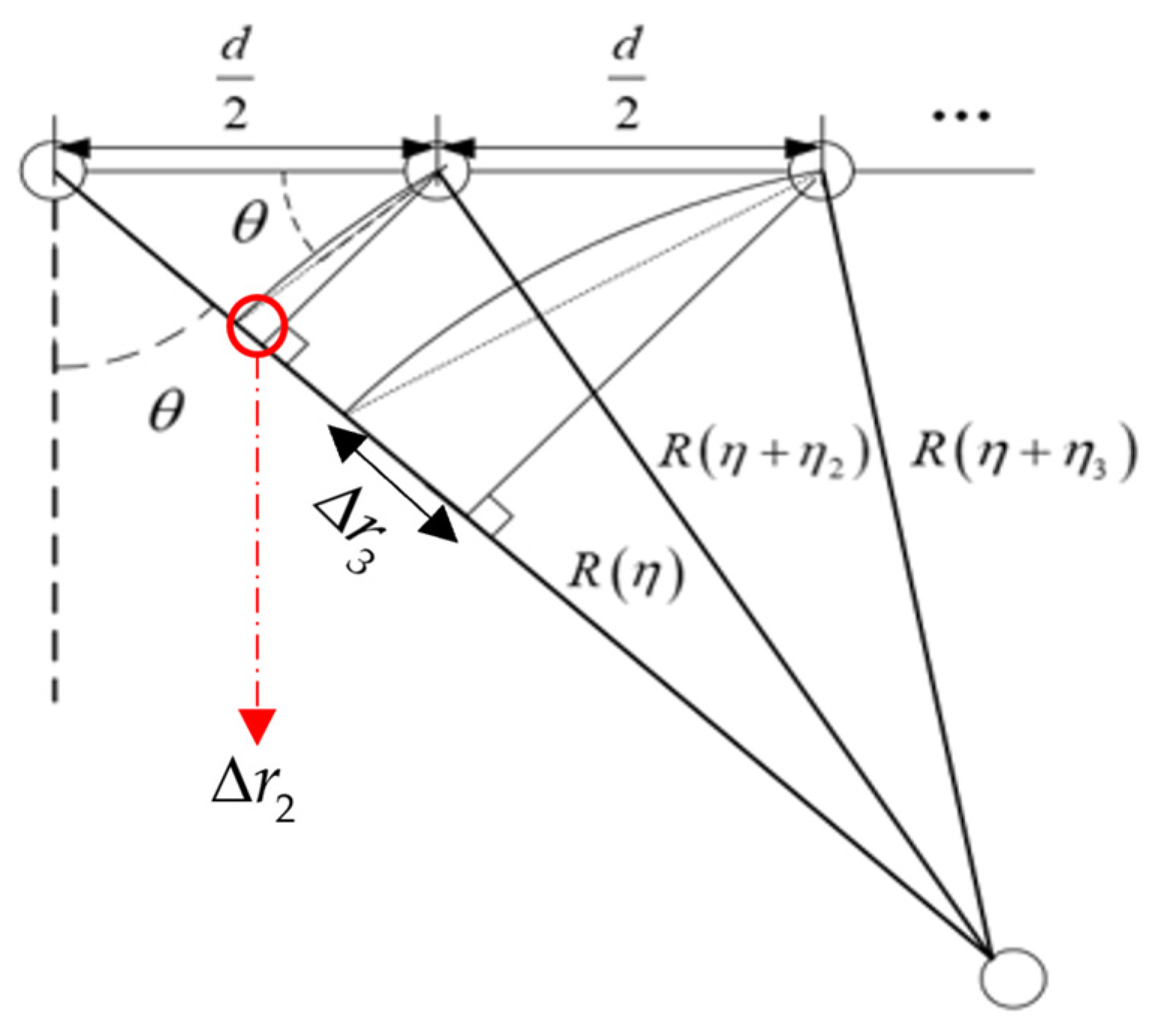
3.1. Parameter Estimation

Suppressive interference does not require precise radar localisation; it can produce broadband noise interference of significant power from either the main lobe or side lobes, effectively covering the entire swath and thereby reducing the signal-to-noise ratio (SNR) of the SAR image to obscure the true target image. By exploiting the power difference between the interference and target signals, parameter estimation techniques can be used to estimate the direction of arrival (DOA) of the interference signal, providing directional parameters for interference suppression.
The echo data from each channel consist of a combination of the interference signal and the target signal, which are incoherent with each other. As can be seen from Equation (11), the original interference signal received by each channel at each slow time is consistent, with the interference angle information reflected in the phase differences between channels due to path differences. Applying a logarithmic transformation to the channel echo data can reduce the amplitude influence of the original data and concentrate the information on the phase. The echo model after logarithmic transformation can be expanded using a Taylor series around the zero point, giving the following expression:
ln ( x i ( τ ) ) = ln ( z i ( τ ) + J i ( τ ) ) ln ( J i ( τ ) ) + z i ( τ ) J i ( τ )
In the above equation, x i ( τ ) represents the echo data of the i-th channel at a given slow time moment, where z i ( τ ) denotes the target echo data, and J i ( τ ) represents the interference echo data. Under strong interference conditions, the target signal is completely overwhelmed by the interference signal, so the above approximation is valid. The ratio between the target signal and the interfering signal approaches zero. Therefore, only the interfering signal component needs to be considered. Further expansion of the interfering term gives the following:
ln ( J m ( τ ) ) = ln ( U 0 + U n ( τ ) ) + j ( 2 π f j τ + φ ( τ ) 2 k π ) + j ( 2 π d m sin ( θ j ) λ 2 k m π )
where k = f l o o r ( ( 2 π f j τ + φ ( τ ) ) / 2 π ) , k m = f l o o r ( d m sin ( θ j ) / λ ) . Equation (24) exhibits 2π periodicity due to the de-periodisation process within the logarithmic transformation, which leads to a bias in the estimation of the interference’s instantaneous phase. At the present slow time, the amplitude and phase information of the spurious signal are identical. Due to the phase differences generated by the path differences at the time of reception on different channels, when adjacent channels are cancelled, the real part relating to the amplitude component and the phase information of the interference signal itself in the imaginary part are cancelled. Only the phase term related to the DOA of the interference remains in the imaginary part.
ϕ = j ( 2 π d sin ( θ j ) λ 2 ( k m k m 1 ) π )
At this point, parameter estimation can be performed to obtain multiple values of θj. By averaging these multiple estimated values, outliers can be removed.

3.2. Interference Reconstruction And Cancellation Method

Traditional spatial filtering is achieved by suppressing interfering signals while allowing the target signal to pass through the spatial filter without distortion. To preserve the integrity of the target signal, the spurious signal is reconstructed without distortion by the spatial filter. The phase information between the channels is then used to reconstruct the interfering signals received by each channel. The complete target signal can be obtained by cancelling the reconstructed interference from the original echo signal. Subsequent spectral reconstruction can still use data from all channels to suppress Doppler ambiguity. The detailed procedure is shown in Figure 5.
As shown in the figure, the reconstructed interference signal is phase-compensated between channels and cancelled with the echo data of each channel to achieve interference suppression. The reconstructed network is then used to reconstruct the spectrum and eliminate the Doppler ambiguity.
Several adaptive beamforming algorithms for spatial domain filtering have been shown to be effective. First, consider the conventional beamforming method, which does not use echo data. In essence, it acts as a matched filter that simultaneously accumulates signals in the main lobe direction. This approach is straightforward to implement and relies on array geometry and arrival angle. The optimal weights should satisfy the following conditions:
{ w o p t a ( θ d ) = 0 w o p t a ( θ j ) = 1
For signals arriving from direction θ j , they pass through without distortion, while signals from other directions are suppressed. If the echo information is not considered, the optimal weights w o p t 1 can be directly obtained using the least-squares method from the constrained equation.
w o p t 1 = g C H ( C C H ) 1
The constraint matrix is defined as C = [ a ( θ d 1 ) a ( θ d 2 ) a ( θ j ) ] . Here, a ( θ d ) is the steering vector for the target, and a ( θ j ) is the steering vector for the interference. The constraint constant vector is g = [ 0   0   0     0   1 ] H . However, conventional DBF involves beam formation in a predetermined direction that does not depend on the characteristics of the received signal for dynamic adjustment. This beamforming method relies heavily on array geometry and phase matching techniques to ensure that the signal is amplified in certain directions and suppressed in others. Adaptive DBF, on the other hand, is able to dynamically adjust the shape and direction of the beam according to the actual conditions of the received signal. This method analyses the collected signals, derives the optimal beamforming weights based on the results of the analysis and then obtains the beam results to adjust the weight vectors of each antenna element in real time to optimise specific performance metrics. The optimal beamforming approach is then considered based on the available information, which includes the known arrival directions of the jammers and the original data from each channel. The covariance matrix of the jammers is unknown. The Linearly Constrained Minimum Variance (LCMV) beamforming algorithm can be used to design a spatial filter that robustly reconstructs the original interference signals. LCMV is a commonly used anti-interference technique in array signal processing, and its criterion can be characterised as follows:
{ min w w H R x x w s . t . w H C = g
where Rxx is the autocorrelation matrix of the received signal, C is the constraint matrix, w is the weight vector and g is the constraint vector. Using the Lagrange multiplier method, the expression for the optimal weight vector is given by the following:
w o p t = R x x 1 C ( C H R x x 1 C ) 1 g
The optimal weights are then used to perform a weighted sum across all channels to reconstruct the noise-suppressed interference signal at the current slow time η k The reconstructed interference signal for the reference channel is expressed as follows:
J k ˜ = w o p t x ( η , τ ) | η = η k
The reconstructed reference interference signal is phase compensated due to the differential propagation path between each channel and the reference channel, resulting in interference echoes for each channel. These echoes are then cancelled against the original echoes from each channel to achieve interference suppression, resulting in the target signal echoes with suppressed interference. This method of interference suppression, which essentially forms nulls in the direction of the interference, does not involve any loss of spatial degrees of freedom. If the system encounters multiple Doppler ambiguities, this approach can provide additional spatial degrees of freedom for azimuthal spectrum reconstruction, thus ensuring the effectiveness of Doppler ambiguity suppression. It should be noted, however, that the restoration and subsequent cancellation of the main lobe cannot completely eliminate the phase compensation introduced by the interference. This residual interference signal, after spectrum reconstruction and azimuth pulse compression, can result in strip suppression in the vicinity of the jammer. As the intensity of the interference increases, strip suppression near the jammer will continue to deteriorate.

3.3. Channel Grouping Nulling Method

The Channel Grouping Nulling (CGN) method, unlike the Interference Reconstruction And Cancellation (IRC) method discussed in the previous section, directly suppresses interference in the spatial domain by nulling. Nulling in the direction of the incoming interference signal is the simplest spatial filtering technique for interference cancellation. However, in order to preserve the phase relationships between the target signals across different channels and to maintain spatial degrees of freedom for azimuth spectrum reconstruction after interference suppression, a sliding grouping of all channels is implemented. Each group undergoes independent interference cancellation. This approach not only effectively mitigates interference, but also preserves multiple degrees of freedom and integrity of the target signals. As a result, the original phase relationships of the target echoes are preserved across all channels. The specific principle is illustrated in Figure 6.
Channels are grouped, and signal suppression is achieved using filter banks for each group. The constraint matrix for each group remains consistent and is expressed as C 1 = [ a ( θ d 1 ) a ( θ d 2 ) a ( θ j ) ] . Due to the change in the phase of the reference channels caused by the channel division, the reference channels of each group will become the first channel of each group. After suppression, the output echo data of the first channel of each group are obtained. In order to implement the anti-jam suppression with the spatial domain filter, the zero-trapping processing should be applied to the signal from the θ d direction while allowing the signal from the θ j direction to pass without loss. The steering vector in the spatial domain is approximately equal to g 1 = [ 1   1   1     1   0 ] H . The optimal values of the weights that correspond to the filter should satisfy this criterion.
{ w o p t a ( θ d ) = 1 w o p t a ( θ j ) = 0
It should be noted that, at this stage, the reduction in the number of elements used to construct nulls per group leads to a broadening of the main beam lobe, a reduction in angular resolution and a reduction in the performance of the constructed matched filter. As a result, the residual noise leakage on both sides of the nulls in the filter also increases. For the optimal beamforming method using echo data, continuing to apply the Linearly Constrained Minimum Variance (LCMV) criterion will result in minimising the output power of the target data at that instant, effectively reducing the image signal-to-noise ratio (SNR) and thus failing to achieve the expected interference suppression effect. As the number of elements available per group increases, the improvement in angular resolution increases the interference suppression effect. However, this comes at the cost of losing more spatial degrees of freedom, which inevitably leads to suboptimal spectral reconstruction and increased levels of ghost images caused by Doppler ambiguity.
To increase the upper limit of this scheme’s ability to suppress Doppler ambiguity, the Minimum Mean Square Error (MMSE) algorithm is introduced to address the issue of poor interference suppression in scenarios with fewer grouped elements. Optimal prediction and filtering are achieved by solving the Wiener–Hopf equation. Interference suppression is realised by minimising the mean square value of the error between the desired output signal d(t) and the actual output signal y(t). The error signal is expressed as ε ( t ) = d ( t ) w H x ( t ) , and the objective function becomes the following:
min w J ( w ) = min w E [ | ε ( t ) | 2 ]
To construct the constraint conditions, we introduce the constraint that the desired signal should pass through the filter without distortion, while the interference should be suppressed. This can be formulated as follows:
{ min w J ( w ) s . t   w H C 1 = g 1
The first equation ensures that the desired signal passes through without distortion, while the second equation minimises the mean square error between the desired signal and the actual output signal. To solve for w, we can combine these equations using Lagrange multipliers:
L ( w , μ ) = E [ | d ( t ) w H x ( t ) | 2 ] μ ( w H C g )
By denoting r x d = E [ x ( t ) d ( t ) ] as the cross-correlation vector between the received signal vector x ( t ) and the desired signal d(t), the optimal weight vector is obtained as follows:
w o p t _ C G N = R x x 1 r x d + 1 2 R x x 1 C 1 ( C 1 H R x x 1 C 1 ) 1 ( g 1 C 1 H R x x 1 r x d )
When high-order multipath interference is present in the echo, this scheme can still effectively suppress interference, but the effect of frequency spectrum superposition results in suboptimal multipath interference suppression. When the number of N-order Doppler ambiguities in the echo satisfies N M N g r o u p + 1 , this scheme can balance interference suppression and Doppler ambiguities suppression. Here, M is the total number of channels, N g r o u p is the number of sub-array channels and the degrees of freedom lost is N g r o u p 1 . The effectiveness of interference suppression improves as the number of sub-array channels increases. Thus, the advantage of this scheme lies in its ability to rationally allocate degrees of freedom resources according to the ambiguity situation. This scheme shows significant superiority under conditions of low-order Doppler ambiguities.

4. Simulation Verification and Analysis

In order to validate the effectiveness of the proposed interference suppression method, a series of simulation experiments are conducted in this section to evaluate the performance of the proposed scheme. The feasibility of the suppression method is verified through point target simulation experiments, and the suppression effects in complex scenarios are demonstrated through distributed target experiments. The point target simulation is presented in Section 4.1. Subsequently, scenario simulations and performance analyses are carried out in Section 4.2, respectively.

4.1. Point Targets Simulation

In this section, we perform simulations on an eight-channel AMPC SAR system operating in stripmap mode. The system parameters are listed in Table 1.
To validate the effectiveness of the proposed algorithm under intense interference conditions, a scenario with five point targets and one jammer is configured, as shown in Figure 7 (units: metres). The interference signal emitted by the jammer is modelled as Gaussian noise and remains constant during each pulse duration. The jammer-to-signal ratio (JSR) is set to 60 dB.
When the pulse repetition frequency (PRF) of the system is 200 Hz, it indicates that there is eight times more aliasing in the target returns. In accordance with the temporal frequency aliasing characteristics, the multiple aliased virtual images can be calculated to have an interval of 150 metres in the direction of θ . The original imaging results are shown in Figure 8a. After adding the suppressive interference, the imaging results are shown in Figure 8b. It can be seen that the point targets in the scene are completely obscured by the interference.
By modifying the PRF, the presence of Doppler ambiguity with different multiples of the PRF can be generated as experimental variables to validate the anti−interference solutions proposed in this paper. As mentioned above, a PRF of 200 Hz corresponds to eight times the Doppler ambiguity multiple, while a PRF of 400 Hz corresponds to four times the Doppler ambiguity multiple. Two methods are used to suppress the interference of the aforementioned Doppler ambiguity echoes, where the channels are grouped into five channels per group, and the imaging results are shown in Figure 9.
Comparing Figure 9a,b as well as Figure 9d,f, it can be seen that the CBF method has comparable anti−interference capabilities to the optimal beamforming method. The differences in the nulls formed by the solved filters at the interference locations can be clearly seen in the subsequent distributed target simulations. Comparing Figure 9b,e, it can be seen that, in scenarios where multiple Doppler ambiguities are present in the echo, the Interference Reconstruction And Cancellation (IRC) method shows superior efficiency in simultaneously suppressing both interference and Doppler ambiguities. Conversely, Channel Grouping Nulling (CGN) results in suboptimal spectrum reconstruction due to the loss of certain degrees of freedom during interference suppression. From Figure 9c,f, it can be seen that, when the Doppler ambiguity in the echoes is relatively low, both the IRC method and the CGN method are able to suppress interference and Doppler ambiguity simultaneously. However, the CGN method does not suffer from the drawback of residual noise interference near the jammer location, which is a notable drawback of the interference recovery cancellation method. This disadvantage becomes more pronounced in distributed target experiments. This indicates that the method retains its effectiveness under less severe conditions of Doppler ambiguity.
To further evaluate the performance of interference suppression in both the azimuth and range directions, two point targets are selected from Figure 9b,f. As shown in Figure 10, the observed performance is consistent with theoretical expectations, providing additional validation of the feasibility of the proposed scheme. This consistency underlines the robustness and reliability of the Interference Reconstruction And Cancellation method under varying conditions.
In addition, a detailed analysis of the matching performance of all five targets is performed by calculating key metrics such as Peak Side Lobe Ratio (PSLR), Integrated Side Lobe Ratio (ISLR) and resolution in both azimuth and range directions. These parameters, as shown in Table 2, provide a comprehensive assessment of the effectiveness of the method in maintaining image quality and accuracy.
From the azimuth and range sections of the point targets, it can be seen that the energy of the interference is significantly reduced after the implementation of interference suppression, allowing the point targets to be clearly distinguished. Comparing the metrics before and after interference suppression in the table, it is observed that the PSLR and ISLR for each target are approximately −13 dB and −9 dB, respectively, indicating that all targets can be restored to a state almost identical to the non-jammed state. As can be seen from Figure 10a and the corresponding data in the table, the residual noise energy in the vicinity of the jammer location is significantly higher than in other areas after interference cancellation. The PSLR of the point targets located closer to the jammer is also higher than that of the targets located further away from the jammer. In terms of resolution, the interference cancellation method maintains a high level of resolution, whereas the resolution of the Channel Grouping Nulling method is decreased.

4.2. Distributed Targets Simulation

The point target simulation only analyses the interference suppression effect on point targets within the scene. To evaluate the performance of the proposed method in a distributed scenario, the following steps involve distributed target simulation to analyse the interference suppression effect in a complex background as well as the differences in the scene near the jammer. Initially, complex scene echoes are generated using ICS, which utilises real radar images and predetermined scene parameters to produce the required raw echo data. The simulation parameters are consistent with those in Table 1, with the jammer position remaining unchanged. The unambiguous echoes of the complex scene are downsampled to obtain the Doppler-ambiguous echo data for each channel. Subsequently, the generated multichannel interference echoes are added to the echo data of each channel. The results of multichannel imaging for both the interference-free scene image and the scene with added interference are shown in Figure 11.
Figure 11b reveals that the useful information is obscured by noise. By adjusting the interference intensity and the Doppler ambiguity multiples in the echo data, different simulation environments are created. Subsequently, interference suppression is performed using the Interference Reconstruction And Cancellation method and the Channel Grouping Nulling method, with conventional beamforming techniques also employed for comparison. The results are illustrated in Figure 12.
From Figure 12a–c,g–i, it can be seen that conventional beamforming, which relies solely on the array structure, maintains a nearly constant interference suppression capability despite changes in the interference environment. However, the excessively wide nulls formed during interference suppression result in the loss of a significant amount of target information, which severely affects the readability of the images. Figure 12d,e show that the interference is effectively suppressed, and the image information is largely recovered. Due to the azimuthal modulation applied to the image, a dark band is formed in the vicinity of the jammer, making some target information unrecognisable and slightly affecting the readability of the image. This demonstrates that the IRC method can effectively restore the original image in the presence of severe Doppler ambiguity and low interference intensity in the echo. In Figure 12f, it can be seen that at relatively high interference intensities, residual strip interference, shown in the figure as a red dotted box, remains in the area near the jammer after suppression using the IRC method. In Figure 12j, numerous bright streaks are observed, which are virtual images caused by suboptimal spectrum reconstruction. This confirms the drawback of the CGN method, which is unable to effectively cancel both Doppler ambiguity and interference at the same time when there is strong Doppler ambiguity in the echo. From Figure 12k,l, it can be seen that, under conditions of low Doppler ambiguity, the CGN method results in less loss of target information, which significantly improves image readability. To quantify the performance of the interference suppression methods, the Root Mean Square Error (RMSE) of the output is used as a metric to evaluate the results. The RMSE is defined as follows:
R E M E = X X * X
where X is the normalised real echoes, and X * is the normalised recovered echoes. A smaller RMSE indicates a better result. The degree of image distortion in Figure 12e,f,j,k is quantified using the RMSE metric, as shown in Table 3. Under severe Doppler ambiguity, the Interference Reconstruction And Cancellation method can effectively restore the image under conditions with a low jammer-to-signal ratio (JSR). However, in high-JSR conditions, it may affect the readability of the image near the jammer. In scenarios with mild Doppler ambiguity, the channel grouping notch method can effectively suppress both interference and Doppler ambiguity, thereby restoring the HRW image.

5. Discussion

The advantage of multichannel Synthetic Aperture Radar (SAR) is that it provides spatial degrees of freedom that can be used for interference suppression. However, the AMPC SAR system also requires spatial information to resolve the range–azimuth ambiguity. Therefore, the study of anti-interference methods for AMPC SAR systems requires a balance in the allocation of degrees of freedom between interference suppression and image reconstruction. Various anti-interference schemes have been designed based on the presence of Doppler ambiguity in the echoes, and two complementary approaches are proposed.
In Section 4, a simple point target simulation is initiated with five targets placed within the scene. Different scenarios are then configured to process the signals using the proposed schemes. The simulation results show that both schemes maintain high levels of performance in their respective applicable scenarios, effectively suppressing interference and accurately recovering point target information. In addition, the Peak Side Lobe Ratio (PSLR), Integral Side Lobe Ratio (ISLR) and resolution in the azimuth and range directions for the five targets are calculated, and the matching performance of all targets is analysed. All metrics are in line with our theoretical expectations.
Further simulations with distributed targets show that both the interference cancellation scheme and the channel grouping notch scheme effectively suppress interference in complex scenarios within the SAR system. This study demonstrates the effectiveness of using digital beamforming (DBF) for azimuth modulation, which mitigates the effects of interference while preserving the integrity of target signals. A comparison of different beamforming methods shows that traditional beamforming, which relies solely on the spatial structure of the array, results in wider dark notches at the interferer locations, leading to greater loss of real target scene data and reduced image readability. The Interference Reconstruction And Cancellation method can maximise its advantages when there is strong Doppler ambiguity in the echoes and the interference intensity is low. However, when the interference intensity is high, the phase compensation introduced by the cancellation process results in residual interference energy manifesting itself as strip noise near the jammer, which can still obscure certain target scenes in the vicinity of the jammer. The Channel Grouping Nulling scheme is suitable for scenarios where the Doppler ambiguity in the echoes is relatively low. By sacrificing a degree of freedom, the system gains the ability to suppress both Doppler ambiguity and interference simultaneously. Furthermore, the effectiveness of the interference suppression is not affected by the intensity of the interference.
A common drawback of both schemes is the loss of useful target information near the interferer due to azimuth modulation, which causes both schemes to fail when the interferer is within the desired target scene. Future research must integrate semi-parametric methods to constrain real target scenes and use algorithms to compensate for the limitations of spatial filtering to achieve a balance between interference suppression and target signal fidelity.
In conclusion, this study provides valuable insights into the performance of interference suppression methods in SAR systems, highlighting the trade-offs and potential of different techniques. By building on these findings and exploring new research directions, more robust and effective interference suppression solutions can be developed to cope with increasingly complex and challenging environments.

6. Conclusions

In order to mitigate the effects of the suppressive interference signals on the AMPC SAR, an interference suppression scheme is proposed which relies on the severity of Doppler ambiguity in the echoes. First, the spatial parameters of the interference signal are estimated by the difference in power between the interference signal and the target signal. Then, if multiple Doppler ambiguities are present in the echoes, the interference is suppressed using the Interference Reconstruction And Cancellation (IRC) method. This method reconstructs the interfering signal and then compensates for the phase difference between the channels to achieve interference cancellation. If Doppler ambiguity suppression does not require excessive degrees of freedom, the Channel Grouping Nulling (GNC) method can be used, sacrificing some degrees of freedom to group channels and achieve nulling suppression of the interference signals. Finally, by reconstructing the remaining signals, an equivalent, uniformly sampled signal with an unambiguous spectrum can be obtained. After imaging, the HRWS SAR image after interference suppression was recovered. The feasibility of the proposed scheme is demonstrated by simulations of point and distributed targets. The calculated imaging performance indicators such as PSLR, ISLR and resolution for point targets meet the theoretical requirements. However, the proposed scheme has the disadvantage of losing target information in the vicinity of the jammer. Future research should attempt to combine semi-parametric methods to suppress interference while preserving the true target scene information near the jammer. In addition, our current research only considers the case of a single jammer, and future studies should address the effective suppression of interference in the presence of multiple jammers.

Author Contributions

Conceptualisation, Z.X. and F.H.; methodology, Z.X., F.H. and Z.S.; formal analysis, F.H. and Z.S.; resources, F.H. and Z.S.; data curation, Z.X. and Z.Z.; writing—original draft preparation, Z.X.; writing—review and editing, Z.X. and F.H.; supervision, F.H. All authors have read and agreed to the published version of the manuscript.

Funding

This research was funded by the National Natural Science Found of China, grant number 42205142.

Data Availability Statement

Data is contained within the article. All data in this paper are generated by simulation and the details have been presented in Section 4.

Acknowledgments

The authors would like to express their gratitude to the editors and the anonymous reviewers for their painstaking efforts and invaluable help, which were of significance to the outcome of this manuscript.

Conflicts of Interest

The authors declare no conflicts of interest.

References

  1. Moreira, A.; Prats-Iraola, P.; Younis, M.; Krieger, G.; Hajnsek, I.; Papathanassiou, K.P. A tutorial on synthetic aperture radar. IEEE Geosci. Remote Sens. Mag. 2013, 1, 6–43. [Google Scholar] [CrossRef]
  2. Li, N.; Lv, Z.; Guo, Z. Pulse RFI Mitigation in Synthetic Aperture Radar Data via a Three-Step Approach: Location, Notch, and Recovery. IEEE Trans. Geosci. Remote Sens. 2022, 60, 5225617. [Google Scholar] [CrossRef]
  3. Dong, Z.; He, F.; Jin, G.; Sun, Z.; Zhang, Y. Performance investigation on elevation cascaded digital beamforming for multidimensional waveform encoding SAR imaging. J. Radars 2020, 9, 828. [Google Scholar]
  4. Chen, J.; Xiong, R.; Yu, H.; Xu, G.; Xing, M. Nonparametric Full-Aperture Autofocus Imaging for Microwave Photonic SAR. IEEE Trans. Geosci. Remote Sens. 2024, 62, 5214815. [Google Scholar] [CrossRef]
  5. Krieger, G.; Gebert, N.; Moreira, A. Multidimensional waveform encoding: A new digital beamforming technique for synthetic aperture radar remote sensing (Article). IEEE Trans. Geosci. Remote Sens. 2008, 46, 31–46. [Google Scholar] [CrossRef]
  6. Bucciarelli, M.; Pastina, D.; Cristallini, D.; Sedehi, M.; Lombardo, P. Integration of Frequency Domain Wideband Antenna Nulling and Wavenumber Domain Image Formation for Multi-Channel SAR. Int. J. Antennas Propag. 2016, 2016, 2834904. [Google Scholar] [CrossRef]
  7. Sun, Z.; Leng, X.; Zhang, X.; Xiong, B.; Ji, K.; Kuang, G. Ship Recognition for Complex SAR Images via Dual-Branch Transformer Fusion Network. IEEE Geosci. Remote Sens. Lett. 2024, 21, 4009905. [Google Scholar] [CrossRef]
  8. Dong, J.; Zhang, Q.; Lu, W.; Cheng, W.; Liu, X. Hybrid Domain Efficient Modulation-Based Deceptive Jamming Algorithm for Nonlinear-Trajectory Synthetic Aperture Radar. Remote Sens. 2023, 15, 2446. [Google Scholar] [CrossRef]
  9. Tang, C.; Ding, J.; Qi, H.; Zhang, L. Smart forwarding deceptive jamming distribution optimal algorithm. IET Radar Sonar Navig. 2024, 18, 953–964. [Google Scholar] [CrossRef]
  10. Ling, Q.; Huang, P.; Wang, D.; Xu, H.; Wang, L.; Liu, X.; Liao, G.; Sun, Y. Range Deception Jamming Performance Evaluation for Moving Targets in a Ground-Based Radar Network. Electronics 2023, 12, 1614. [Google Scholar] [CrossRef]
  11. Liu, Y.-X.; Zhang, Q.; Xiong, S.-C.; Ni, J.-C.; Wang, D.; Wang, H.-B. An ISAR Shape Deception Jamming Method Based on Template Multiplication and Time Delay. Remote Sens. 2023, 15, 2762. [Google Scholar] [CrossRef]
  12. Zhao, B.; Zhou, F.; Bao, Z. Deception Jamming for Squint SAR Based on Multiple Receivers. IEEE J. Sel. Top. Appl. Earth Obs. Remote Sens. 2015, 8, 3988–3998. [Google Scholar] [CrossRef]
  13. Huang, H.-X.; Zhou, Y.-Y.; Jing, W.; Huang, Z.-T. A frequency-based inter/intra partly coherent jamming style to SAR. In Proceedings of the 2010 2nd International Conference on Signal Processing Systems, Dalian, China, 5–7 July 2010. [Google Scholar]
  14. Tao, M.; Su, J.; Huang, Y.; Wang, L. Mitigation of radio frequency interference in synthetic aperture radar data: Current status and future trends. Remote Sens. 2019, 11, 2438. [Google Scholar] [CrossRef]
  15. Wang, W.; Wu, J.; Pei, J.; Sun, Z.; Yang, J.; Yi, Q. Antirange-Deception Jamming from Multijammer for Multistatic SAR. IEEE Trans. Geosci. Remote Sens. 2022, 60, 5212512. [Google Scholar] [CrossRef]
  16. Tao, M.; Zhou, F.; Zhang, Z. Wideband Interference Mitigation in High-Resolution Airborne Synthetic Aperture Radar Data. IEEE Trans. Geosci. Remote Sens. 2016, 54, 74–87. [Google Scholar] [CrossRef]
  17. Queiroz de Almeida, F.; Younis, M.; Krieger, G.; Moreira, A. Multichannel Staggered SAR Azimuth Processing. IEEE Trans. Geosci. Remote Sens. 2018, 56, 2772–2788. [Google Scholar] [CrossRef]
  18. Sikaneta, I.; Gierull, C.H.; Cerutti-Maori, D. Optimum Signal Processing for Multichannel SAR: With Application to High-Resolution Wide-Swath Imaging. IEEE Trans. Geosci. Remote Sens. 2014, 52, 6095–6109. [Google Scholar] [CrossRef]
  19. Wang, Y.; Liu, Y.; Li, Z.; Suo, Z.; Fang, C.; Chen, J. High-Resolution Wide-Swath Imaging of Spaceborne Multichannel Bistatic SAR with Inclined Geosynchronous Illuminator. IEEE Geosci. Remote Sens. Lett. 2017, 14, 2380–2384. [Google Scholar] [CrossRef]
  20. Currie, A.; Brown, M.A. Wide-swath SAR. Proc. Inst. Elect. Eng.-Radar Sonar Navigat. 1992, 139, 122–135. [Google Scholar] [CrossRef]
  21. Kim, J.-H.; Younis, M.; Gabele, M.; Prats, P.; Krieger, G. First Spaceborne Experiment of Digital Beam Forming with TerraSAR-X Dual Receive Antenna Mode. In Proceedings of the European Radar Conference, Chengdu, China, 24–27 October 2011. [Google Scholar]
  22. Kim, J.H.; Younis, M.; Prats-Iraola, P.; Gabele, M.; Krieger, G. First spaceborne demonstration of digital beamforming for azimuth ambiguity suppression. IEEE Trans. Geosci. Remote Sens. 2012, 51, 579–590. [Google Scholar] [CrossRef]
  23. Jing, W.; Xing, M.; Qiu, C.W.; Bao, Z.; Yeo, T.S. Unambiguous reconstruction and high-resolution imaging for multiple-channel SAR and airborne experiment results. IEEE Geosci. Remote Sens. Lett. 2009, 6, 102–106. [Google Scholar] [CrossRef]
  24. Chen, Z.; Zhang, Z.; Qiu, J.; Zhou, Y.; Wang, W.; Fan, H.; Wang, R. A Novel Motion Compensation Scheme for 2-D Multichannel SAR Systems with Quaternion Posture Calculation. IEEE Trans. Geosci. Remote Sens. 2021, 59, 9350–9360. [Google Scholar] [CrossRef]
  25. Chang, S.; Deng, Y.; Zhang, Y.; Zhao, Q.; Wang, R.; Zhang, K. An Advanced Scheme for Range Ambiguity Suppression of Spaceborne SAR Based on Blind Source Separation. IEEE Trans. Geosci. Remote Sens. 2022, 60, 5230112. [Google Scholar] [CrossRef]
  26. Huang, Y.; Zhao, B.; Tao, M.; Chen, Z.; Hong, W. Review of synthetic aperture radar interference suppression. J. Radars 2020, 9, 86–106. [Google Scholar]
  27. Yu, J.; Li, J.; Sun, B.; Chen, J.; Li, C.; Li, W.; Xu, L. Single RFI Localization Based on Conjugate Cross-Correlation of Dual-Channel Sar Signals. In Proceedings of the IGARSS 2019–2019 IEEE International Geoscience and Remote Sensing Symposium, Yokohama, Japan, 28 July–2 August 2019. [Google Scholar]
  28. Lin, X.-H.; Xue, G.-Y.; Liu, P.-G. Novel data acquisition method for interference suppression in dual-channel SAR. Prog. Electromagn. Res. 2014, 144, 79–92. [Google Scholar] [CrossRef]
  29. Rosenberg, L.; Gray, D. Anti-jamming techniques for multichannel SAR imaging. Radar Sonar Navig. IEE Proc. 2006, 153, 234–242. [Google Scholar] [CrossRef]
  30. Yu, C.; Zhang, Y.; Yu, A.; Dong, Z.; Liang, D. Terrain scattered interference suppression for multichannel SAR. In Proceedings of the International Asia-pacific Conference on Synthetic Aperture Radar, Seoul, Reoublic of Korea, 26–30 September 2011; IEEE: Piscatvey, NJ, USA, 2011. [Google Scholar]
  31. Bollian, T.; Osmanoglu, B.; Rincon, R.; Lee, S.K.; Fatoyinbo, T. Adaptive Antenna Pattern Notching of Interference in Synthetic Aperture Radar Data Using Digital Beamforming. Remote Sens. 2019, 11, 1346. [Google Scholar] [CrossRef]
  32. Cerutti-Maori, D.; Sikaneta, I. A Generalization of DPCA Processing for Multichannel SAR/GMTI Radars. IEEE Trans. Geosci. Remote Sens. 2013, 51, 560–572. [Google Scholar] [CrossRef]
  33. Rongbing, G. Rebound Jamming Suppression by Two-Channel SAR. Signal Process. 2005, 21, 27–30. [Google Scholar]
  34. Cheng, S.; Sun, X.; Cai, Y.; Zheng, H.; Yu, W.; Zhang, Y.; Chang, S. A Joint Azimuth Multichannel Cancellation (JAMC) Anti-Barrage Jamming Scheme for Spaceborne SAR. IEEE J. Sel. Top. Appl. Earth Obs. Remote Sens. 2022, 15, 9913–9926. [Google Scholar] [CrossRef]
  35. Huang, Y.; Wen, C.; Chen, Z.; Chen, J.; Liu, Y.; Li, J.; Hong, W. HRWS SAR Narrowband Interference Mitigation Using Low-Rank Recovery and Image-Domain Sparse Regularization. IEEE Trans. Geosci. Remote Sens. 2022, 60, 5217914. [Google Scholar] [CrossRef]
  36. Gebert, N.; Krieger, G.; Moreira, A. Digital Beamforming on Receive: Techniques and Optimization Strategies for High-Resolution Wide-Swath SAR Imaging. IEEE Trans. Aerosp. Electron. Syst. 2009, 45, 564–592. [Google Scholar] [CrossRef]
  37. Bordoni, F.; Younis, M.; Krieger, G. Ambiguity Suppression by Azimuth Phase Coding in Multichannel SAR Systems. IEEE Trans. Geosci. Remote Sens. 2012, 50, 617–629. [Google Scholar] [CrossRef]
Figure 1. Geometric model of the echo signal.
Remotesensing 16 02812 g001
Figure 2. Geometric illustration of the relationship between the other channels and the reference channel.
Remotesensing 16 02812 g002
Figure 3. Schematic diagram of space–time two-dimensional spectrum and Doppler aliasing.
Remotesensing 16 02812 g003
Figure 4. Schematic diagram of spectrum reconstruction using DBF network.
Remotesensing 16 02812 g004
Figure 5. Processing flow of the Interference Reconstruction And Cancellation method.
Remotesensing 16 02812 g005
Figure 6. Illustration of channel grouping for null steering.
Remotesensing 16 02812 g006
Figure 7. Illustration of the point target simulation scenario.
Remotesensing 16 02812 g007
Figure 8. Observed scene. (a) Multichannel image reconstruction without interference; (b) interfer ence with multichannel reconstructed images.
Remotesensing 16 02812 g008
Figure 9. Imaging result of the point target simulation. (a) Result of CBF at 60 dB JSR, PRF = 200 Hz; (b) result of IRC at 60 dB JSR, PRF = 200 Hz; (c) result of IRC at 60 dB JSR, PRF = 400 Hz; (d) results of CBF at 60 dB JSR, PRF = 400 Hz; (e) results of CGN at 60 dB JSR, PRF = 200 Hz; (f) results of CGN at 60 dB JSR, PRF = 400 Hz.
Remotesensing 16 02812 g009
Figure 10. The cross−sections of point targets in the azimuth and range directions. (a) The azimuthal cross−section of the IRC; (b) the range cross−section of the IRC; (c) the azimuthal cross−section of the CGN; (d) the range cross−section of the CGN; (e) partial enlargement of the red dashed box in (a); (f) partial enlargement of the red dashed box in (b); (g) partial enlargement of the red dashed box in (c); (h) partial enlargement of the red dashed box in (d).
Remotesensing 16 02812 g010
Figure 11. Distributed target scene. (a) Interference−free SAR image; (b) interference−polluted SAR image.
Remotesensing 16 02812 g011
Figure 12. The image results of interference suppression. (a) CBF at 40 dB JSR, PRF = 200 Hz; (b) CBF at 40 dB JSR, PRF = 400 Hz; (c) CBF at 60 dB JSR, PRF = 400 Hz; (d) IRC at 40 dB JSR, PRF = 200 Hz; (e) IRC at 40 dB JSR, PRF = 400 Hz; (f) IRC at 60 dB JSR, PRF = 400 Hz; (g) CBF at 40 dB JSR, PRF = 200 Hz; (h) CBF at 40 dB JSR, PRF = 400 Hz; (i) CBF at 60 dB JSR, PRF = 400 Hz; (j) CGN at 40 dB JSR, PRF = 200 Hz; (k) CGN at 40 dB JSR, PRF = 400 Hz; (l) CGN at 60 dB JSR, PRF = 400 Hz.
Remotesensing 16 02812 g012aRemotesensing 16 02812 g012b
Table 1. List of point targets simulation parameters.
ParameterSymbolsValue
Carrier frequency f c 10 GHz
Bandwidth B r 50 MHz
Equivalent baseline d 0.25 m
Number of channels M 8
Nearest slant range R 0 10 km
Platform velocity v 200   m / s
Doppler bandwidth B a 1600 Hz
Platform height h 5 km
Table 2. PSLR, ISLR and resolution of 5 targets.
TargetAzimuth DirectionRange Direction
PSLR
(dB)
ISLR
(dB)
Resolution
(m)
PLSR
(dB)
ISLR
(dB)
Resolution
(m)
Imaging result without
interference
1−13.097−9.7420.125−13.193−9.4762.967
2−13.157−9.7340.125−13.184−9.4642.952
3−13.281−9.7140.125−13.081−9.3583.000
4−13.175−9.7410.125−13.218−9.5093.000
5−13.269−9.7030.125−13.183−9.5052.963
Processing result of IRC method1−13.481−9.7010.125−13.242−9.0433.000
2−13.548−9.6580.125−13.149−9.1322.980
3−13.525−9.5360.125−13.187−8.6632.982
4−13.264−9.5250.125−13.199−9.1342.980
5−13.212−9.6140.125−13.137−9.2553.000
Processing result of CGN method1−13.011−9.3540.163−13.338−9.5742.991
2−13.153−9.8810.163−13.048−9.5763.000
3−13.336−9.5780.163−13.084−9.4573.000
4−13.402−9.5010.163−13.437−9.5912.928
5−13.475−9.7930.163−13.214−9.6263.000
Table 3. Image quality quantification comparison.
MethodExperimental Scenario
Description
REME
Interference Reconstruction And Cancellation (IRC) MethodHigh JSR0.8077
Low JSR0.6512
Channel Grouping Nulling (CGN) MethodHigh-order Doppler
ambiguity
0.7816
Low-order Doppler
ambiguity
0.6051
Disclaimer/Publisher’s Note: The statements, opinions and data contained in all publications are solely those of the individual author(s) and contributor(s) and not of MDPI and/or the editor(s). MDPI and/or the editor(s) disclaim responsibility for any injury to people or property resulting from any ideas, methods, instructions or products referred to in the content.

