The Analysis of North Brazil Current Rings from Automatic Identification System Data and Altimetric Currents

Abstract

This paper aims to analyze the North Brazil Current (NBC) rings during the initial 5 months of 2020 using surface currents derived from Automatic Identification System (AIS) data in comparison with altimetry-based Archiving, Validation and Interpretation of Satellite Oceanographic Data (AVISO) current fields. The region of NBC rings is characterized by relatively high marine traffic, facilitating an accurate current estimation. Our investigation primarily focused on a brief period coinciding with intensive in situ measurements (EUREC4A-OA experiment). The Angular Momentum Eddy Detection and tracking Algorithm (AMEDA) detection algorithm was then employed to detect and track eddies in both fields. Subsequently, a particular NBC ring present in the region in January and February 2020 was examined. The comparison demonstrated that AIS data exhibited the precision and resolution necessary to effectively identify the NBC rings and smaller surrounding eddies, aligning well with other datasets such as in situ measurements, sea surface temperature (SST), and sea surface salinity (SSS) data. Moreover, we established that AIS data yielded accurate regional velocity fields, as evidenced by an analysis of energy spectra. Furthermore, our analysis revealed that AIS data captured aspects of eddy–eddy interactions which were not adequately depicted in AVISO fields.

1. Introduction

The North Brazil Current (NBC) is a western boundary current (WBC) dominating the surface circulation of the Western Tropical North Atlantic ocean (WTNA). It connects the South Equatorial Current (SEC) with the North Equatorial Current (NEC) along the South American continental slope, as illustrated in Figure 1. Near the estuary of the Amazon River between latitudes 6°N–8°N, the NBC loops back upon itself and feeds the North Equatorial Countercurrent [1,2]. At this retroflection, warm-core anticyclonic mesoscale eddies, referred to as NBC rings, detach from the main stream and propagate northwestward towards the Antilles. These eddies have been intensively studied over the past few decades through in situ measurements [2,3,4,5,6,7,8], numerical models [5,9,10], and satellite observations [5,11,12,13,14,15,16,17]. At the time of their formation, NBC rings have an average diameter exceeding 400 km [14]. Their azimuthal velocity reaches approximately 1 m/s. These eddies move northwestward (towards the Antilles) with translation velocities (Ts) ranging from 0.1 m/s to 0.17 m/s (8–15 km/day) for about 3 to 4 months (see Figure 1) [9,10,11,14,18]. Their significant speeds affect the regional oceanic circulation and particularly the shape of the Atlantic Meridional Overturning Circulation (AMOC) [18]. Furthermore, NBC rings also play a crucial role in the broader context of global ocean circulation and climate dynamics as they transport and disperse relatively warm, low-salinity and nutrient-rich water originating from the Amazon river [14]. It is likely that the warm and low-salinity water carried by these eddies enhances the intensity of atmospheric cyclones passing through that area. A study demonstrated that 68% of Category 5 cyclones (the most intense) passed over an NBC ring [19].

In this framework, this work takes advantage of the high-resolution ocean surface current dataset, recently derived from Automatic Identification System (AIS) marine traffic data [20], to examine the NBC rings and the circulation surrounding them during the period spanning from 1 January 2020 to 31 May 2020. The objective was to examine the evolution of NBC rings and their physical properties, based on the detection from AIS data, and to contrast these findings with satellite altimetry data.

This 5-month period was chosen to cover the EUREC4A-OA experiment at sea [21]. This experiment was carried out from mid-January to mid-February 2020, north of Brazil and of the Guyanas, to measure air–sea interactions at the mesoscale and the NBC rings in that region. It involved four ships and four planes, from the USA, Germany, and France. In particular, it yielded data on the NBC ring structure, trajectory, and interaction with neighboring eddies.

The AIS was created under the International Maritime Organization (IMO) convention as a vessel surveillance system that facilitates the exchange of information among ships and shores. Today, the AIS is considered as an essential part of global maritime safety. eOdyn (www.eodyn.com—accessed on 27 July 2024) has repurposed the primary use of the AIS from its original intent as a surveillance system to ocean surface current estimation wherever maritime traffic exists. This emerging potential offered by the global AIS network to complement the existing ocean surface current data has been investigated since 2015 [20,22,23]. The technology behind this kind of current measurements relies on the analysis of ships’ movements from collected AIS messages. Thanks to this transmission system installed on ships, it is possible to almost instantly obtain precious information regarding the sailing status of each vessel: their position, speed, true heading (heading relative to the water surface), as well as the course over the ground. The difference in angle between the true heading and the course over the ground serves as an indicator of the influence of surface currents. This principle is known as ship’s drift [24,25,26]. The method for deducing surface currents from ships’ drift existed long before the AIS era and was used in the 17th century by Gerard De Brahm and in the 18th century by Matthew Fontaine Maury [27] to estimate the intensity and direction of the Gulf Stream current. Richardson [24,25] further refined this method using historical data from the logbooks of military and merchant vessels, although with very limited precision in vessel data. Richardson [26] also demonstrated that the effect of wind on vessels (leeway drift) was negligible as long as the aerodynamic and hydrodynamic drags were of the same order, which is generally the case except for container and passenger ships.

Today, thanks to satellite AIS data, it is possible to obtain near-real-time information on maritime traffic. With over 100,000 commercial ships operating worldwide (https://hbs.unctad.org/merchant-fleet/—accessed on 27 July 2024), each emitting AIS messages at a frequency of up to 10 messages per minute, the volume of data generated is immense. However, current collection systems face technological limitations, preventing the capture of all emitted messages. The number of AIS messages that satellites can receive daily varies significantly, influenced by factors such as satellite capabilities, coverage areas, and vessel density. Consequently, despite the advanced technology in use, not all AIS data can be effectively collected and processed.

Using satellite AIS data, our previous work [20,23] already demonstrated the potential of AIS data streams to retrieve the ocean surface current in a dynamically relevant region such as the Agulhas region, addressing to some extent the limitations of altimetry products.

In this study, we apply the AMEDA to the daily AIS current fields on one hand, and the daily absolute dynamic topography (ADT) maps from satellite altimetry on the other hand, to identify and track in time ocean eddies and NBC rings, in particular to identify their trajectories and associated parameters. In the first part of this study, we use the acquired output form AMEDA to globally assess the ability of AIS data to detect realistic mesoscale eddy-related structures. We then focus on a particular NBC ring that was detected on both fields starting from 1 January 2020 until its dissipation on the second half of February 2020. We provide a complete dynamical description of the eddy as depicted in both datasets. We also compare our results to NBC rings’ parameters from the state-of-the-art literature.

This paper is organized as follows. Section 2 presents the datasets used in this study. The methodology is outlined in Section 3. Section 4 presents the results of our analysis. First, we present the statistics of eddy tracking from AVISO and AIS fields, offering a direct comparison between the two datasets. Subsequently, we focus on tracking an individual NBC ring, comparing statistics of their physical characteristics and spatio-temporal variability as derived from AIS and satellite altimetry data by AMEDA. A discussion and a regionalization of the results is provided in Section 5. Finally, a summary of our work is presented in Section 6.

2. Data

2.1. AVISO/DUACS

In our study, we use the Archiving, Validation and Interpretation of Satellite Oceanographic Data (AVISO) dataset, produced by Collecte Localisation Satellites (CLS) and provided by the European Copernicus Marine Environment Monitoring Service (CMEMS) (https://marine.copernicus.eu/—accessed on 27 July 2024), to compare it with the AIS-derived ocean current product, particularly focusing on eddy activities. This dataset, specifically the “Delayed Time” and “All-Sat merged” versions, incorporates merged data, using an optimal space–time objective analysis [28,29], from multiple altimeter missions, encompassing up to seven concurrent missions [30].

Our analysis employed the gridded format of the AVISO dataset, characterized by a spatial resolution of 0.25° and a temporal resolution of one day, covering the period of January–May 2020. A critical aspect of our work was assessing the dataset’s accuracy in terms of eddy tracking. Although the nominal spatial grid resolution is approximately 25 km, the actual resolution in capturing physical phenomena is likely greater, estimated to be around 65 km, or possibly even more, as indicated by [31]. Additionally, Amores et al. (2018) [32] highlighted that the gridded AVISO dataset may underrepresent the number of eddies, attributing this limitation to its spatial resolution constraints.

2.2. AIS

In this paper, we use ocean surface currents maps derived from space-based AIS data using the methodology described in [20]. Within the domain of study, we analyzed and processed more than 10 million messages provided by Spire Maritime (https://spire.com/maritime/—accessed on 27 July 2024) from 2988 different vessels. Figure 1 displays a map illustrating the density of ship traffic, revealing particularly dense activity, especially within the “eddy boulevard” (highlighted by the red rectangle), which is of importance for this study. The AIS ocean surface currents were then produced on a regular grid with a spatial resolution of 0.125° and temporal resolution of one day. To summarize briefly, the methodology was based on the velocity decomposition principle that can be written as follows:

$${\overrightarrow{V}}_{sog}={\overrightarrow{V}}_{stw}+{\overrightarrow{u}}_{drift}$$

(1)

where $V_{sog}$ is the speed over ground, ${\phi }_{cog}$ the course over ground, $V_{stw}$ the speed through water, ${\phi }_{th}$ the true heading of each vessel considered, ${\overrightarrow{u}}_{drift}$ represents the vessel drift which is primarily due to the ocean surface current (u and v hereafter). This equation can be reformulated as a system of linear equations after projection onto the appropriate axes, specifically the zonal and meridional axes:

$$\begin{array}{c}\hfill \left\{\begin{array}{cc}{V}_{sog}sin\left({\phi }_{cog}\right)=V_{stw}sin\left({\phi }_{th}\right)+u\hfill & \left(\mathrm{zonal}\right)\hfill \\ V_{sog}cos\left({\phi }_{cog}\right)=V_{stw}cos\left({\phi }_{th}\right)+v\hfill & \left(\mathrm{meridional}\right)\hfill \end{array}\right.\end{array}$$

(2)

Among these variables, all, with the exception of $V_{stw}$, are provided within the AIS data messages transmitted by vessels. Consequently, we are presented with a system comprising three unknowns and only two equations. To resolve this, we instead consider n AIS messages received from different vessels within a small space–time window (Refer to Figure 1 for the typical values of n). We assume that the surface current conditions evolve slowly within that window, ensuring that all vessels experience the same underlying surface current. This assumption allows us to reformulate the initial equations into the following linear system:

$$\begin{array}{c}\hfill \left\{\begin{array}{cc}{V}_{so{g}_1}sin\left({\phi }_{co{g}_1}\right)=V_{st{w}_1}sin\left({\phi }_{t{h}_1}\right)\hfill & +u\hfill \\ V_{so{g}_1}cos\left({\phi }_{co{g}_1}\right)=V_{st{w}_1}cos\left({\phi }_{t{h}_1}\right)\hfill & +v\hfill \\ ⋮⋮\hfill & ⋮\hfill \\ V_{so{g}_n}sin\left({\phi }_{co{g}_n}\right)=V_{st{w}_n}sin\left({\phi }_{t{h}_n}\right)\hfill & +u\hfill \\ V_{so{g}_n}cos\left({\phi }_{co{g}_n}\right)=V_{st{w}_n}cos\left({\phi }_{t{h}_n}\right)\hfill & +v\hfill \end{array}\right.\end{array}$$

(3)

Thus, we can express the Equation (3) in the form $Ax=b$, with:

$$\begin{array}{c}\hfill A=\left(\begin{array}{cccccc}1& 0& sin\left({\phi }_{t{h}_1}\right)& 0& \cdots & 0\\ 0& 1& cos\left({\phi }_{t{h}_1}\right)& 0& \cdots & 0\\ ⋮& ⋮& & \ddots \\ 1& 0& 0& \cdots & 0& sin\left({\phi }_{t{h}_n}\right)\\ 0& 1& 0& \cdots & 0& cos\left({\phi }_{t{h}_n}\right)\end{array}\right),x=\left(\begin{array}{c}u\\ v\\ V_{st{w}_1}\\ ⋮\\ V_{st{w}_n}\end{array}\right),b=\left(\begin{array}{c}{V}_{so{g}_1}sin\left({\phi }_{co{g}_1}\right)\\ V_{so{g}_1}cos\left({\phi }_{co{g}_1}\right)\\ ⋮\\ V_{so{g}_n}sin\left({\phi }_{co{g}_n}\right)\\ V_{so{g}_n}^{c}os\left({\phi }_{co{g}_n}\right)\end{array}\right)\end{array}$$

(4)

Despite the seemingly straightforward approach to solving this linear system, several challenges arise. A substantial quantity of data is necessary to obtain realistic average estimates. Without sufficient data, the estimates may not accurately reflect the actual sea surface currents. Furthermore, the hypothesis that vessels within a given spatio-temporal window experience the same current is not always accurate. Currents can vary significantly in space and even more so over time, leading to potential inaccuracies when solving the above system. Additionally, if all vessels are moving in the same direction, the system becomes unstable (badly conditioned matrix A), causing the solution to the equation to diverge. It is also crucial to preprocess and filter the data to eliminate vessels that are maneuvering, as such vessels can introduce noise and errors into the current estimates. Moreover, in the presence of strong winds and/or waves, the estimates of sea surface currents become unreliable. These environmental factors can significantly affect the accuracy of the current estimates and must be considered in the analysis. The detailed approach of data filtering is explained in Le Goff et al. [20]. In addition to that, AIS datasets contain data gaps, particularly in regions with lower traffic, such as the northeastern area of the region of interest (cf. Figure 1). To address this issue, missing data were reconstructed using the optimal interpolation scheme [29].

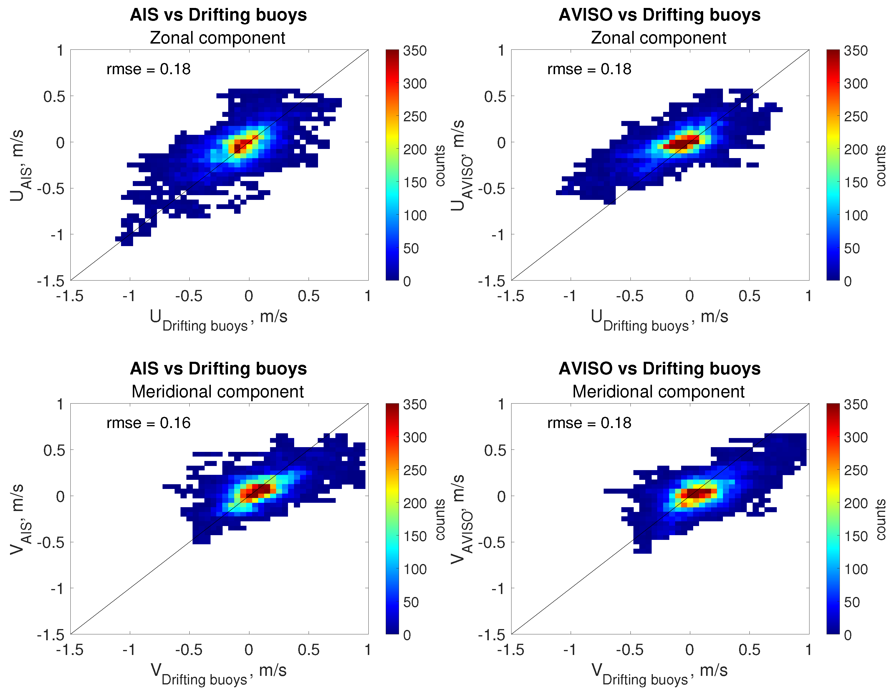
2.3. Assessment of AIS and AVISO Ocean Current Estimates against In Situ Datasets

To assess the accuracy of the AIS and AVISO ocean current estimates, we used the latest version of the hourly dataset from the Global Drifter Program (data available at http://www.aoml.noaa.gov/phod/gdp/hourly_data.php—accessed on 27 July 2024). The dataset comprises horizontal velocity and position estimates at hourly intervals [33] from 22 individual surface drifter trajectories for the study period. Considering the velocities of the drifters as a “ground truth”, we systematically colocated (in both time and space) the velocities associated to the drifting buoys with our estimates from the AIS and those from AVISO. Matchup criteria were set so that the time difference between AIS and AVISO estimates was within one day and the spatial separation was within 10 km.

Figure 2 presents two-dimensional histograms which compare sea surface current estimates from the AIS and AVISO datasets with colocated measurements from drifting buoys. The first row illustrates the zonal component, while the second row depicts the meridional component, with AIS data shown on the left and AVISO data on the right. Notably, the accuracy of both datasets is quite similar when compared to the drifters, with both AIS and AVISO exhibiting a root-mean-square error (RMSE) of 0.18 m/s for the zonal component. Additionally, we observe a relatively slight improvement in RMSE for the AIS meridional component (0.16 m/s vs. 0.18 m/s). Interestingly, for the AVISO zonal component velocities (first row), the lowest absolute values never exceed −0.5 m/s. This, however, is clearly not the case for the AIS zonal estimates, where the absolute values quite regularly exceed −0.5 m/s.

2.4. The EUREC4 A-OA Measurements

During the EUREC4A-OA experiment at sea, the two research ships, R/V L’Atalante and R/V Maria S. Merian, measured the surface oceanic currents with Ship-mounted Acoustic Doppler Current Profilers (S-ADCPs). On both ships, currents down to 1000 m depth were measured with the 38 kHz S-ADCP. On R/V L’Atalante, a 150 kHz S-ADCP provided currents with a higher accuracy but only down to 200 m depth (in practice). On R/V Maria S. Merian, a 75 kHz S-ADCP measured currents down to 800 m depth, again with a better accuracy than the 38 kHz one. The best accuracy on the velocity measurement was the largest of 5% of the sampled velocity or $\pm 0.005$ m/s. With currents of about $0.5$ m/s in the NBC rings, the accuracy was therefore $\pm 0.025$ m/s [12,34].

2.5. Numerical Model

To compare the energy spectra from the AVISO dataset and the AIS with those of a numerical model of the region, we made use of reanalyses of a (1/12)th-of-a-degree-resolution HYCOM model, with 41 vertical levels (a reanalysis of the GOFS3.1 simulation). This hybrid coordinate ocean model assimilated surface data (SSH and SST) and Argo float profiles but not the EUREC4A data. The surface currents were extracted from the model results with a 1-day sampling period.

3. Eddy Detection and Tracking Method

In this study, NBC rings from the AIS-based current and AVISO datasets were identified and tracked in time by the AMEDA detection and tracking algorithm [35]. AMEDA is a hybrid algorithm based on dynamic parameters and geometric properties of the velocity field that detects eddies by identifying minima and maxima on the velocity field and selecting closed streamlines around them. The algorithm also dynamically tracks eddies backward and forward in time. Eddy tracks detected by AMEDA are labeled as anti-cyclonic (AE) or cyclonic (CE) based on their sense of rotation, with physical information on the closed contour of maximum velocity: the eddy lifetime, radius of maximal azimuthal velocity (Rmax), modulus of maximal azimuthal velocity (Vmax), Rossby number (Ro), eddy kinetic energy (EKE), amplitude, translation speed (Ts), and covered distance. The main advantage of the AMEDA tracking algorithm is also its ability to capture multiple eddy interaction events such as merging and splitting events.

This detection was applied to 5 months (1 January 2020–31 May 2020) of AIS current fields and the “all-sat-merged” series of delayed time daily ADT maps gridded at 1/4° in the NBC region [−62°E–52°E; 6°N–15°N].

Note that we obtained similar detection and tracking of eddies when comparing AMEDA with the TOEddies detection and tracking algorithm [36,37].

4. Results

4.1. Eddy Tracking Statistics

Table 1. The number of individual eddies and the associated number of trajectories in the AIS and AVISO datasets. These results are based on trajectories lasting at least 7 days. Shorter trajectories were excluded from the analysis.

		AIS	AVISO
Individual eddies (snapshots)	Total	821	900
	AE	520 (64%)	450 (50%)
	CE	301 (36%)	450 (50%)
Trajectories (dynamic view)	Total	48	43
	AE	25 (52%)	20 (46%)
	CE	23 (48%)	23 (55%)

shows the number of detected individual eddies and the associated number of trajectories in the AIS and AVISO datasets within the region of interest and during the time period of the analysis. Only trajectories that lasted at least 7 days were included and all shorter trajectories were excluded from the analysis. This value was slightly smaller than the altimetry mapping decorrelation time of 10 days [38]. It is important to clarify that the term “individual eddy” refers to the singular manifestation of either a cyclonic or anticyclonic structure identified at a specific location on a given daily map. Conversely, an eddy track denotes the continuous trajectory of an eddy throughout its temporal existence. Following the restriction above, the algorithm detected more individual eddies from the AVISO fields than from the AIS ($9\%$ more). Conversely, more trajectories were detected within the AIS fields (48 vs. 43). For the individual AVISO eddy numbers, the cyclonic (CEs) and anticyclonic Eddies (AEs) had a balanced contribution, each comprising 50% of the total count, whereas for the AIS fields, the AEs represented more than two-thirds of the individual eddies. In particular, this indicated that AEs were longer lived than CEs. Also, the AIS AE trajectories outnumbered the AVISO AE’s by 5 (25 vs. 20). The number of CE trajectories was the same in the two datasets.

4.2. Individual NBC Ring Tracking

In this section, our attention turns to an anticyclonic eddy located in the NBC region. This eddy is an NBC ring, formed near the Amazon estuary in the Atlantic Ocean through the retroflexion of the NBC. Here, we examine its spatial and physical properties from AMEDA as depicted by the two datasets, AIS and AVISO. This particular eddy was observable from early January 2020 until its definitive dissipation on 16 February 2020. It retained our attention due to its persistent presence during the EUREC4A-OA oceanographic campaign (http://eurec4a-oa.eu/—accessed on 27 July 2024), which sampled it via several sections.

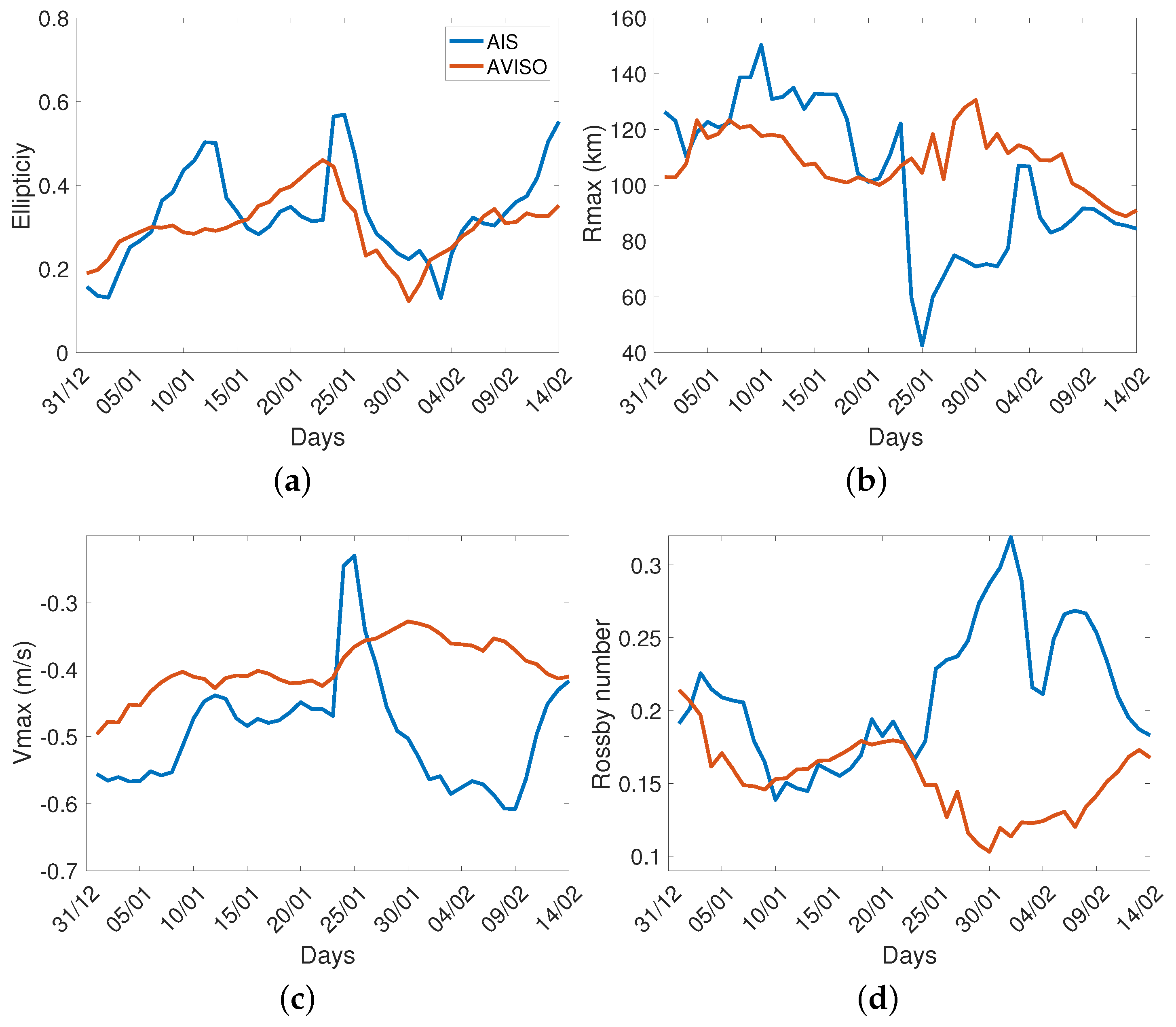
4.2.1. Statistics of Physical NBC Characteristics Derived from AIS and Satellite Altimetry Data

In this section, we computed the average parameters (translation speed, Rmax, Vmax, and Ro) for the NBC ring during all the time steps when it was inside the region of interest. The outcomes of this analysis and results from previous studies are summarized in

Table 2. Statistics of physical NBC characteristics derived from AIS and satellite altimetry data compared with results from previous studies using different measurement methods.

Par	AIS	AVISO	Historical Values
Ts	0.18 m/s	0.14 m/s	0.15, 0.16, 0.15, 0.16, 0.15, 0.14, 0.17, 0.17 m/s [6,7,11,12,13,14,15,17]
Rmax	102 km	110 km	124 km, 140, 140 km [12,16,17]
Vmax	0.5 m/s	0.4 m/s	0.45, 0.4, 0.8, 0.42, 1, 0.75, 0.9, 0.37, and 0.40 [2,4,5,8,11,12,16,17,18]
Ro	0.20	0.15	0.17, 0.08, [0.12 and 0.26], 0.33 [5,8,12,16]

. It is important to note that the parameters provided for both AIS and AVISO datasets represent the average values computed throughout their duration within the study area. This differs from the state-of-the-art reference parameters, which were derived from averaging over an extended period encompassing various detected rings within the region. The comparison of these values show that the measurements via AIS and AVISO fit in the range of historical data but for its radius of maximal velocity; a reason for this is proposed below.

• Translation speed

AMEDA estimates for the AIS NBC ring translation speed showed that it varied from a minimum of 0.04 m/s to a maximum of 0.45 m/s, with an average value of 0.18 m/s (15.50 km/day). AVISO values, on the other hand, varied from 0.03 m/s to 0.22 m/s, with an average value of 0.14 m/s. For comparison, different methods yielded translation speeds of 0.15, 0.16, 0.15, 0.16, 0.15, 0.14, 0.17, and 0.17 m/s, as reported in [6,7,11,12,13,14,15,17], respectively.

• Rmax

The analyses of the AIS NBC ring radius Rmax provided an average value of 102 km, with a minimum of 42 km and a maximum of 130 km. For the AVISO ring, we observed significantly less variability in Rmax during the tracking time period, with an average value of 110 km. The minimum and the maximum were found to be, respectively, 88 km and 130 km. Results from the EUREC4A-OA campaign [12] provided an average value of 123.9 (±23.3) km, with a minimum of 65 km and a maximum of 179.8 km. Results from previous studies [16,17] provided relatively larger values for Rmax (i.e., bigger structures), with an average value around 140 km. However, their analyses may have been based on measurements performed at the time of maximal sea level anomaly (SLA) for each ring, potentially coinciding with periods of higher Rmax values.

• Vmax

The minimum and maximum values of the mean azimuthal velocities corresponding to the AIS ring were 0.23 m/s and 0.6 m/s, respectively, while the mean value for Vmax was 0.5 m/s. AVISO found a lower mean value of Vmax of 0.4 m/s. The corresponding minimum and maximum values were found to be 0.32 m/s and 0.5 m/s, respectively. During the EUREC4A-OA campaign [12], a mean azimuthal value of 0.45 (±0.11) m/s was reported. Among other studies, different methods yielded a Vmax mean of 0.4, 0.8, 0.42, 1, 0.75, 0.9, 0.37, and 0.40 m/s, as reported in [2,4,5,8,11,16,17,18], respectively.

• Ro

Finally, the Rossby number of the selected NBC ring from the AIS varied from a minimum of 0.14 to a maximum of 0.32, with an average value of 0.20. In comparison, the AVISO ring presented a lower Rossby number ranging from 0.10 to 0.21 with an average value of 0.15. The Rossby number is defined as the ratio of inertial to Coriolis forces in a rotating fluid system, relying on the Coriolis parameter f, which decreases near the Equator. Consequently, within this region, Ro values are higher than those observed in regions situated farther from the equatorial belt. In comparison, ref. [12] found during the EUREC4A-OA campaign that rings possessed an average Rossby number of 0.17 (±0.03), with values ranging from a minimum of 0.08 to a maximum of 0.27. Different methods yielded various values of 0.08, between 0.12 and 0.26, and 0.33, as reported in [5,8,16], respectively.

4.2.2. Temporal Variability of Physical NBC Characteristics Derived from AIS and Satellite Altimetry Data

The detailed trajectory of the NBC eddy, as detected and tracked by AMEDA, is depicted in Figure 3. The trajectories (black for AIS and magenta for AVISO) correspond to the centers of the closed contour detected from the velocity fields. The set of daily contours corresponding to Rmax and Vmax is displayed for each configuration. Despite the trajectory from the AVISO dataset being relatively smoother than that from the AIS dataset, both trajectories are close and superimposed. The smoothness of the AVISO trajectory arises from the fact that the product uses Level 3 along-tracks altimetric data that are spatially and temporally optimally interpolated to create a complete grid [28,31]. This interpolation smoothes out the currents and, consequently, the eddies detected by AMEDA. This is not the case for currents derived from AIS data, which are temporally resolved more efficiently due to the significant maritime traffic in the Eddy Boulevard region (cf. Figure 1).

In both fields, the eddy moved (quasi) westward, at a latitude of 9°, for the period between the 1st and the 25th of January, then northwestward for the rest of its lifetime, at a relatively constant speed of about 15.5 km/day (equivalent to 0.18 m/s), which was relatively low compared to its maximum azimuthal speeds Vmax ranging (on average) between 0.4 and 0.5 m/s from both fields. Overall, the AIS ring demonstrated greater variability in its characteristic size when contrasted with the AVISO ring, which maintained a more stable size and translation speed throughout the lifespan of the eddy. From Figure 4b, we can divide the analysis into two parts.

Until the 15th of January 2020, the NBC ring from AIS data had an average diameter of approximately 260 km (Rmax ≈ 130 km), notably larger in size compared to that from AVISO data (≈240 km). During that period, the AVISO ring’s diameter slightly decreased to reach its minimum value of 200 km between 15 and 20 January, just prior to shifting its direction towards the northwest.

Conversely, the AIS eddy experienced a sudden drop in its diameter around the 25th of January, reaching 80 km, which then gradually increased until reaching 160 km, ultimately matching the size observed for the AVISO eddy by mid-February. The NBC ring eventually weakened in the second half of February before colliding with the Lesser Antilles, where the eddy broke up and dissipated by interaction with the topography [2,9,10,11,18]. The eddy vanished from the AIS map on February 17th, but it remained visible on the AVISO dataset for an additional week, approximately corresponding to the altimetry mapping decorrelation time.

The general shape of an eddy can be compared to that of an ellipse, with an ellipticity parameter defined as $e=|1-b/a|$, where a and b represent the major and minor axes, respectively. Thus, when ellipticity approaches zero (resp., one), the shape of the eddy is purely circular (resp., elliptical). The ellipticity parameter also serves to characterize the stability of an eddy, as a more circular shape indicates greater stability [39]. As illustrated in Figure 4a, both the AIS and AVISO current datasets exhibited variable ellipticity parameters ranging from 0.1 (quasi-circular) to 0.6 (highly elliptical).

Based on the ellipticity parameter, five key phases in the life cycle of the NBC ring could be distinguished. In the initial phase (0–6 days), the eddy displayed a predominantly circular form ($e<0.3$), with approximately the same values for both AIS and AVISO rings, with notable high azimuth velocity Vmax and radius Rmax characteristics (Figure 4b,c). Subsequently (6–15 days), the AIS eddy became more elliptical, contrasting with the AVISO ring, while maintaining a low Rossby number (≈0.16). Moving into the third phase (15–21 days), both eddies exhibited similar and significant ellipticity ($e>0.2$) and a low Rossby number. Phase four (22–35 days) was characterized by a sharp rise and fall in ellipticity for both eddies. In the AIS currents, the eddy bifurcated at its maximum ellipticity before merging with another eddy to regain a circular form. These merging and splitting events are discussed in the next section. Notably, the Rossby number peaked at approximately 0.32 for the AIS ring. The final phase (35–47 days) marks the weakening and eventual disappearance of the eddies, with the AIS eddy vanishing first, displaying a higher ellipticity towards the end of its lifetime. During this phase, the Rossby number, as well as the other parameters of the two eddies, tended to converge once again.

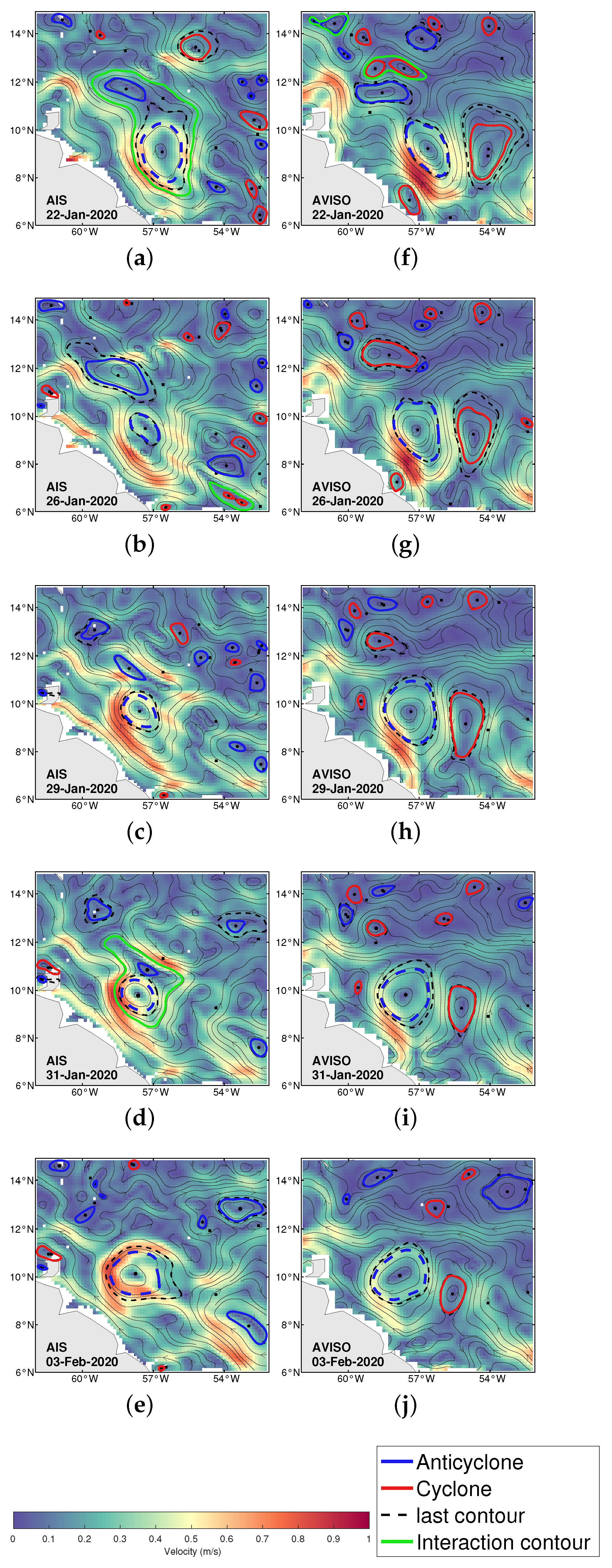
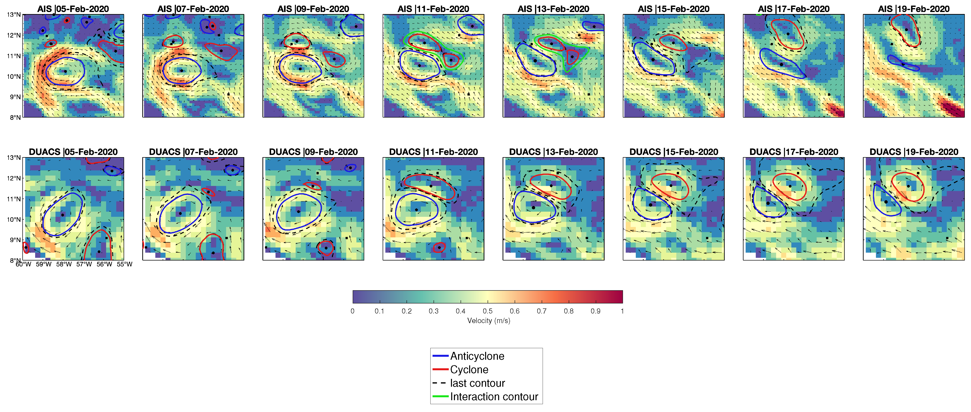
4.3. Spatio-Temporal Variability of the NBC Ring as Derived from AMEDA

To further investigate the NBC ring characteristics, we focused on the eddies’ interactions during the considered time period. Figure 5 shows the AMEDA detection of AE (blue) and CE (red) eddies, within the region of interest, at five different days spanning from 22 January to 3 February. Around 22 January, the NBC ring observed in both the AIS and AVISO data tended to be trapped into an northwestward-flowing jet along the coast. This jet originated from the north of the eddy for the AIS field and further to the northeast for the AVISO field. In both cases, the jet engulfed the NBC ring on its southern side (map of 22 January on Figure 5), then headed towards the Antilles. This shape for the jet is unusual [27] as it generally follows the coast of South America. However, the NBC ring was clearly elliptical with a major axis in the meridional direction (in both fields), suggesting that a jet meander existed and created the necessary shear. The ellipticity parameter of the NBC ring then became significant (0.45 for AVISO and 0.55 for AIS), and its stability was compromised. The dynamics of the two fields were still very close at that stage, but the AIS and AVISO current fields and the underlying NBC ring started to behave differently thereafter. The AVISO data were more straightforward to analyze. The jet coming from the east appeared to have two sources. The first one was located around 12°N. The second and more intense source was located in the southeast (52°W, 7°N), which then moved northward to merge with and reinforce the first source. As the jet approached the NBC ring, it split into two branches, one passing north of the ring along a perfectly zonal path, the second branch reaching the NBC ring to its southeast before ascending towards the northwest. This stable situation, which allowed the NBC ring to progressively regain a more circular shape (e < 0.1), remained unchanged throughout the entire period.

However, the configuration was different for the NBC ring in the AIS field. On January 26th, similar to the AVISO data, one of the jet sources was located in the eastern part of the area around 12°N. However, another source was located north of the ring. Consequently, the two jets merged and circulated around the NBC ring as shown in Figure 5b. This circulation was different from that visible on the AVISO field as the northern quasi-zonal flow (at 12°) (Figure 5g–j) was absent. Given this configuration, the NBC ring was stretched, and its ellipticity increased (Figure 4a). On January 24, 25, and 26, the NBC ring in the AIS field split into two smaller eddies visible in Figure 5b. AMEDA observed a sudden decrease in the radius Rmax and the mean azimuthal velocity of the NBC ring (Figure 4b,c). In fact, a splitting event occurred as the AMEDA map shows a contour encompassing these two vortices (black dashed lines). Subsequently, another anticyclone, which had been detected in the AIS current field since 19 February, approached the NBC ring on 29 and 31 January (Figure 5c,d), ultimately merging with it on 2 February. The NBC ring absorbed some of the energy from this anticyclone, resulting in an increase in its radius and azimuthal velocity. Finally, it regained a more circular shape. Note also that there was a closed contour around the two eddies on 22 January. This contour is represented by a green line in Figure 5a. This closed circulation gradually tightened, ultimately corresponding to the merger of the two anticyclonic eddies. This merging event was responsible for very strong currents over a short distance, resulting in a significant Rossby number.

Finally, on 3 February, both current fields exhibited an NBC ring of similar size, position, and deformation, though the currents are relatively different.

Another significant process, not present in the AVISO data but solely detected through the AIS data, near the NBC ring in February involved the merging of two cyclones. This particular merging event is shown in Figure 6 through consecutive snapshots taken intermittently from February 5th to February 19th of ocean surface datasets derived from the AIS (top panel) and altimetry (lower panel). From February 1st to 5th, snapshots revealed the gradual approach of the two cyclones towards each other, resulting in the formation of a connected region by 11 February, as indicated by the black dashed curve detected by AMEDA. Subsequently, they begin to aggregate, forming a larger eddy. On February 11th, only a single eddy is observed in the snapshot, confirming the occurrence of cyclone merging. On the AVISO side, AMEDA began detecting the cyclonic eddy from February 7th, which continued to grow in size following the same trajectory as the AIS eddy, without showing any merging event.

5. Discussion

The previous section showed how useful the AIS data were to study NBC rings. More generally, we wished to validate the quality of AIS data, and their realism at a regional scale, by computing energy spectra.

Figure 7 shows the power spectra of sea surface velocities (kinetic energy spectra) for the rotational part of the AIS velocities (called OS rot), the AVISO geostrophic velocities, and the rotational velocities from a HYCOM model simulation (called Hycom rot) at a $\left({\displaystyle \frac{1}{12}}\right)$th-degree resolution. The nonlinearity of this HYCOM simulation with altimetric data assimilation allowed the generation of smaller scale features than rings. The usual $k^{-3}$ spectrum of two-dimensional turbulence in the inertial range of enstrophy cascade [40,41,42] was recovered for scales larger than 250 km. Note that that scale was comparable with the Rhines scale of turbulence on the beta-plane [43]. Indeed $L_{Rh}=\sqrt{U/\beta }$, which provides, with typical values of the current in the region ($U=1$ m/s) and $\beta \approx 2{10}^{-11}$/(m.s), $L_{Rh}\approx 225$ km. A slope discontinuity appeared at that scale, yielding a steeper spectrum $E\left(k\right)\approx k^{-4}$ down to scales of about 80 km. Indeed, the presence of developed vortices in turbulence rendered the spectra steeper than $k^{-3}$ [44,45,46,47]. This spectrum steeper than predicted by the phenomenological theory could also be related to the presence of vorticity filaments [48]. For even shorter scales, ($25<L<80$ km), while the AVISO data joined the phenomenological spectrum (mostly due to energy spreading between scales via data interpolation), the AIS velocity spectrum remained in agreement with the high-resolution HYCOM simulation. This evidenced the presence of stronger vorticity gradients in these latter results than in AVISO’s.

The observations made on the last figure drew us towards a joint analysis of the normalized vertical vorticity and normalized lateral strain rate [49]. The steepness of the energy spectrum with the AIS data reflected clear-cut vorticity fronts. Joint statistics of the normalized vertical vorticity $\zeta /\mathrm{f}=(v_x-u_y)/\mathrm{f}$ and normalized lateral strain rate $\alpha /\mathrm{f}=\left(\sqrt{{[u_x-v_y]}^2+{[v_x+v_y]}^2}\right)/\mathrm{f}$ are shown in Figure 8, where $u_x$ and $u_y$ (respectively, $v_x$ and $v_y$) are the derivatives of the zonal (respectively, meridional) component with respect to the x-axis and y-axis. f is the Coriolis parameter. The plots show how different the vorticity and strain distributions were between the AIS and AVISO data: the AIS data indicated (on average) stronger values of vorticity, with a slight bias towards negative values (i.e., more anticyclonic eddies), and stronger values of the (negative) strain rate. Again, this is in agreement with more intense and sharper flow features in AIS data.

To complement this point, we present orthoradial velocity profiles of the NBC ring for 5 January 2020 and 3 February 2020, as determined by AMEDA from AIS and AVISO data (Figure 9). These profiles correspond to the mean velocity averaged along each closed streamline (starting from the eddy center) as a function of the mean radius. The blue and red profiles correspond to the mean values ($\langle R\rangle ;\langle V\rangle$) computed from AVISO and AIS data, respectively, while colored dashed ones are obtained from the following cyclogeostrophic equation [50] with different values of Coriolis frequencies.

$$\langle V\rangle =-{\displaystyle \frac{\mathrm{f}\langle R\rangle }{2}}(1-\sqrt{1+{\displaystyle \frac{4\langle V_g\rangle }{\mathrm{f}\langle R\rangle }}})$$

(5)

where f is the Coriolis parameter, $V_g$ is the geostrophic velocity profile corresponding to the AVISO products, and $\langle R\rangle$ is the mean radius. This cyclogeostrophic correction is essential for intense large-scale anticyclones, as the geostrophic balance—crucial for deriving surface velocity from altimetric data—may not hold true and could significantly underestimate their intensity. In Figure 9, the AIS velocities are clearly faster than those obtained by AVISO and, on the left-hand subplot, they correspond better to a cyclogeostrophic balance. This is consistent with the higher Ro observed with AIS data for the NBC ring. On the right-hand subplot, the AIS eddy velocities are again much larger than those provided by AVISO, but they appear now in excess of those corresponding to a cyclogeostrophic balance. This may be related to too smooth sea-surface height (SSH) gradients.

Another quality check (and usefulness validation) of the AIS data at the regional scale is provided by the comparison between the AIS currents and SSS or SST maps (see Figure 10). The left-hand column indicates—but for a small anomaly at 9°N–57°W—how well the freshwater plume from the Amazon River is advected by the velocity field, and in particular, how it is funneled along the coast, inshore of the NBC rings. Further west, this freshwater circulates anticyclonically around the western NBC rings—at 10°${30}^{\prime }$N–57°W.

Concerning SST, in the right-hand column, two strong horizontal gradients are noticed, one between the coast and the NBC, or its ring, and one between the latter and the offshore waters. The warm waters are clearly enclosed in streamlines of AIS currents, in particular in the NBC rings.

From January 27 to 29, 2020, the R/V L’Atalante conducted an eastward zonal section of the NBC ring at 9.4°N, utilizing, among other instruments, ADCP profilers (Figure 11—Section 5). Subsequently, from February 12 to 13, the R/V L’Atalante traversed the ring again (Figure 11—Section 32), shortly before the R/V Maria S Merian sampled it on 14 February (Figure 11—Section 28) and 15 February (Figure 11—Section 29). These sections yielded high-resolution observations of the vertical structure of the ring. Clearly, two features appeared on the four sections: (1) the velocity was intensified above a 100 m depth, but the L’Atalante sections which were more accurate vertically (due to the use of the 150 kHz ADCP) also showed a weaker secondary intensification of the current below a 150 m depth; (2) there was a notable vertical tilt of the NBC rings, at least for the two L’Atalante sections, and for the Merian Section 28. This tilt can be interpreted either as the effect of the NBC ring propagation, of the interaction with another surface eddy, or as the superposition of a surface ring with a subsurface ring. All sections showed velocity moduli at least in the $[-0.5,+0.5]$ m/s range. Peaks at $\pm 1$ m/s were observed on the earliest section (L’Atalante Section 5). Such values were mentioned earlier for NBC ring rotational velocities [2]. We can also note that the locations of velocity maxima provided by the AVISO and AIS data were satisfactory and mostly corresponded to the location of the surface velocity maxima, when the rings were vertically tilted. Concerning the Maria S. Merian data, the agreement was slightly better with AVISO than with AIS for that position.

6. Conclusions

In areas of intense commercial navigation, the AIS data are sufficiently dense spatially to accurately reproduce the ocean currents at a regional scale and at a mesoscale, with a good similarity to numerical ocean models (such as HYCOM). In particular, they show intense currents and intense velocity gradients which are not displayed by AVISO geostrophic currents. Even though the SWOT satellite will provide high-resolution surface currents in the near future, these currents will still be geostrophic. The AIS data provide the whole current and in particular, the divergent flow. This can be used to validate the estimates of Ekman currents or of wave currents.

Our study evidenced that AIS data were precise enough and well resolved to identify the NBC rings, and smaller, surrounding eddies, in good agreement with other data (in situ measurements, SST data). Subsequently, we showed that AIS data provided accurate velocity fields regionally (in terms of energy spectra).

The AIS are also dense in time in these regions. This allows the tracking of the NBC rings in time and the determination of their trajectories and their deformation along these trajectories. Furthermore, this deformation can be related in part to eddy–eddy interactions, which are properly described with the AIS dataset but not observed in AVISO fields.

Our study was focused on a short time span, around a period of intensive in situ measurements (EUREC4A-OA experiment). Further work will indicate, on a longer run, if the statistical characteristics and properties of eddies are better reproduced with AIS data in this region (and in the Arabian Sea), where maritime traffic is sufficient to provide high-resolution, high-frequency data on ocean currents.

References

1. Cushman-Roisin, B.; Tang, B.; Chassignet, E.P. Westward motion of mesoscale eddies. J. Phys. Oceanogr. 1990, 20, 758–768. [Google Scholar] [CrossRef]
2. Fratantoni, D.M.; Richardson, P.L. The evolution and demise of North Brazil Current rings. J. Phys. Oceanogr. 2006, 36, 1241–1264. [Google Scholar] [CrossRef]
3. Johns, W.E.; Lee, T.N.; Schott, F.A.; Zantopp, R.J.; Evans, R.H. The North Brazil Current retroflection: Seasonal structure and eddy variability. J. Geophys. Res. Ocean. 1990, 95, 22103–22120. [Google Scholar] [CrossRef]
4. Richardson, P.; Hufford, G.; Limeburner, R.; Brown, W. North Brazil current retroflection eddies. J. Geophys. Res. Ocean. 1994, 99, 5081–5093. [Google Scholar] [CrossRef]
5. Fratantoni, D.M.; Johns, W.E.; Townsend, T.L. Rings of the North Brazil Current: Their structure and behavior inferred from observations and a numerical simulation. J. Geophys. Res. Ocean. 1995, 100, 10633–10654. [Google Scholar] [CrossRef]
6. Garzoli, S.L.; Ffield, A.; Yao, Q. North Brazil Current rings and the variability in the latitude of retroflection. In Elsevier Oceanography Series; Elsevier: Amsterdam, The Netherlands, 2003; Volume 68, pp. 357–373. [Google Scholar]
7. Sharma, N.; Anderson, S.P.; Brickley, P.; Nobre, C.; Cadwallader, M.L. Quantifying the seasonal and interannual variability of the formation and migration pattern of North Brazil Current Rings. In Proceedings of the OCEANS 2009, Bremen, Germany, 11–14 May 2009; pp. 1–7. [Google Scholar]
8. Castelão, G.; Johns, W. Sea surface structure of North Brazil Current rings derived from shipboard and moored acoustic Doppler current profiler observations. J. Geophys. Res. Ocean. 2011, 116. [Google Scholar] [CrossRef]
9. Garraffo, Z.D.; Johns, W.E.; Chassignet, E.P.; Goni, G.J. North Brazil Current rings and transport of southern waters in a high resolution numerical simulation of the North Atlantic. In Elsevier Oceanography Series; Elsevier: Amsterdam, The Netherlands, 2003; Volume 68, pp. 375–409. [Google Scholar]
10. Jochumsen, K.; Rhein, M.; Hüttl-Kabus, S.; Böning, C.W. On the propagation and decay of North Brazil Current rings. J. Geophys. Res. Ocean. 2010, 115, C10004. [Google Scholar] [CrossRef]
11. Didden, N.; Schott, F. Eddies in the North Brazil Current retroflection region observed by Geosat altimetry. J. Geophys. Res. Ocean. 1993, 98, 20121–20131. [Google Scholar] [CrossRef]
12. Subirade, C.; L’Hégaret, P.; Speich, S.; Laxenaire, R.; Karstensen, J.; Carton, X. Combining an Eddy Detection Algorithm with In-Situ Measurements to Study North Brazil Current Rings. Remote Sens. 2023, 15, 1897. [Google Scholar] [CrossRef]
13. Goni, G.J.; Johns, W.E. A census of North Brazil Current rings observed from TOPEX/POSEIDON altimetry: 1992–1998. Geophys. Res. Lett. 2001, 28, 1–4. [Google Scholar] [CrossRef]
14. Fratantoni, D.M.; Glickson, D.A. North Brazil Current ring generation and evolution observed with SeaWiFS. J. Phys. Oceanogr. 2002, 32, 1058–1074. [Google Scholar] [CrossRef]
15. Mélice, J.L.; Arnault, S. Investigation of the intra-annual variability of the North Equatorial Countercurrent/North Brazil Current eddies and of the instability waves of the North tropical Atlantic Ocean using satellite altimetry and Empirical Mode Decomposition. J. Atmos. Ocean. Technol. 2017, 34, 2295–2310. [Google Scholar] [CrossRef]
16. Aroucha, L.; Veleda, D.; Lopes, F.; Tyaquiçã, P.; Lefèvre, N.; Araujo, M. Intra-and inter-annual variability of North Brazil current rings using angular momentum Eddy detection and tracking algorithm: Observations from 1993 to 2016. J. Geophys. Res. Ocean. 2020, 125, e2019JC015921. [Google Scholar] [CrossRef]
17. Bueno, L.F.; Costa, V.S.; Mill, G.N.; Paiva, A.M. Volume and Heat Transports by North Brazil Current Rings. Front. Mar. Sci. 2022, 9, 831098. [Google Scholar] [CrossRef]
18. Johns, W.E.; Zantopp, R.J.; Goni, G.J. Cross-gyre transport by North Brazil Current rings. In Elsevier Oceanography Series; Elsevier: Amsterdam, The Netherlands, 2003; Volume 68, pp. 411–441. [Google Scholar]
19. Ffield, A. Amazon and Orinoco River plumes and NBC rings: Bystanders or participants in hurricane events? J. Clim. 2007, 20, 316–333. [Google Scholar] [CrossRef]
20. Le Goff, C.; Boussidi, B.; Mironov, A.; Guichoux, Y.; Zhen, Y.; Tandeo, P.; Gueguen, S.; Chapron, B. Monitoring the greater Agulhas Current with AIS data information. J. Geophys. Res. Ocean. 2021, 126, e2021JC017228. [Google Scholar] [CrossRef]
21. Stevens, B.; Bony, S.; Farrell, D.; Ament, F.; Blyth, A.; Fairall, C.; Karstensen, J.; Quinn, P.K.; Speich, S.; Acquistapace, C.; et al. EUREC4A. Earth Syst. Sci. Data 2021, 13, 4067–4119. [Google Scholar] [CrossRef]
22. Guichoux, Y.; Lennon, M.; Thomas, N. Sea surface currents calculation using vessel tracking data. In Proceedings of the Maritime Knowledge Discovery and Anomaly Detection Workshop, Joint Research Centre, Ispra, Italy, 5–6 July 2016. [Google Scholar]
23. Benaïchouche, S.; Legoff, C.; Guichoux, Y.; Rousseau, F.; Fablet, R. Unsupervised reconstruction of sea surface currents from ais maritime traffic data using trainable variational models. Remote Sens. 2021, 13, 3162. [Google Scholar] [CrossRef]
24. Richardson, P.L.; McKee, T. Average seasonal variation of the Atlantic equatorial currents from historical ship drifts. J. Phys. Oceanogr. 1984, 14, 1226–1238. [Google Scholar] [CrossRef]
25. Richardson, P.; Reverdin, G. Seasonal cycle of velocity in the Atlantic North Equatorial Countercurrent as measured by surface drifters, current meters, and ship drifts. J. Geophys. Res. Ocean. 1987, 92, 3691–3708. [Google Scholar] [CrossRef]
26. Richardson, P.L. Drifting in the wind: Leeway error in shipdrift data. Deep. Sea Res. Part I Oceanogr. Res. Pap. 1997, 44, 1877–1903. [Google Scholar] [CrossRef]
27. Brown, J. Ocean Circulation: Prepared by an Open University Course Team; Elsevier: Amsterdam, The Netherlands, 2016. [Google Scholar]
28. Le Traon, P.; Nadal, F.; Ducet, N. An improved mapping method of multisatellite altimeter data. J. Atmos. Ocean. Technol. 1998, 15, 522–534. [Google Scholar] [CrossRef]
29. Bretherton, F.P.; Davis, R.E.; Fandry, C. A technique for objective analysis and design of oceanographic experiments applied to MODE-73. In Deep Sea Research and Oceanographic Abstracts; Elsevier: Amsterdam, The Netherlands, 1976; Volume 23, pp. 559–582. [Google Scholar]
30. SSALTO/DUACS User Handbook: (M) SLA and (M) ADT Near-Real Time and Delayed Time Products. 2013. Available online: https://www.aviso.altimetry.fr/fileadmin/documents/data/tools/hdbk_duacs.pdf (accessed on 27 July 2024).
31. Ballarotta, M.; Ubelmann, C.; Pujol, M.I.; Taburet, G.; Fournier, F.; Legeais, J.F.; Faugère, Y.; Delepoulle, A.; Chelton, D.; Dibarboure, G.; et al. On the resolutions of ocean altimetry maps. Ocean. Sci. 2019, 15, 1091–1109. [Google Scholar] [CrossRef]
32. Amores, A.; Jordà, G.; Arsouze, T.; Le Sommer, J. Up to what extent can we characterize ocean eddies using present-day gridded altimetric products? J. Geophys. Res. Ocean. 2018, 123, 7220–7236. [Google Scholar] [CrossRef]
33. Elipot, S.; Lumpkin, R.; Perez, R.C.; Lilly, J.M.; Early, J.J.; Sykulski, A.M. A global surface drifter data set at hourly resolution. J. Geophys. Res. Ocean. 2016, 121, 2937–2966. [Google Scholar] [CrossRef]
34. L’Hégaret, P.; Schütte, F.; Speich, S.; Reverdin, G.; Baranowski, D.B.; Czeschel, R.; Fischer, T.; Foltz, G.R.; Heywood, K.J.; Krahmann, G.; et al. Ocean cross-validated observations from R/Vs L’Atalante, Maria S. Merian, and Meteor and related platforms as part of the EUREC4A-OA/ATOMIC campaign. Earth Syst. Sci. Data 2023, 15, 1801–1830. [Google Scholar] [CrossRef]
35. Le Vu, B.; Stegner, A.; Arsouze, T. Angular Momentum Eddy Detection and tracking Algorithm (AMEDA) and its application to coastal eddy formation. J. Atmos. Ocean. Technol. 2018, 35, 739–762. [Google Scholar] [CrossRef]
36. Chaigneau, A.; Gizolme, A.; Grados, C. Mesoscale eddies off Peru in altimeter records: Identification algorithms and eddy spatio-temporal patterns. Prog. Oceanogr. 2008, 79, 106–119. [Google Scholar] [CrossRef]
37. Chaigneau, A.; Eldin, G.; Dewitte, B. Eddy activity in the four major upwelling systems from satellite altimetry (1992–2007). Prog. Oceanogr. 2009, 83, 117–123. [Google Scholar] [CrossRef]
38. Dibarboure, G.; Pujol, M.I.; Briol, F.; Traon, P.L.; Larnicol, G.; Picot, N.; Mertz, F.; Ablain, M. Jason-2 in DUACS: Updated system description, first tandem results and impact on processing and products. Mar. Geod. 2011, 34, 214–241. [Google Scholar] [CrossRef]
39. Han, G.; Dong, C.; Yang, J.; Sommeria, J.; Stegner, A.; Caldeira, R.M. Strain Evolution and Instability of an Anticyclonic Eddy From a Laboratory Experiment. Front. Mar. Sci. 2021, 8, 645531. [Google Scholar] [CrossRef]
40. Kraichnan, R.H. Inertial Ranges in Two-Dimensional Turbulence. Phys. Fluids 1967, 10, 1417–1423. [Google Scholar] [CrossRef]
41. Batchelor, G.K. Computation of the Energy Spectrum in Homogeneous Two-Dimensional Turbulence. Phys. Fluids 1969, 12, II-233–II-239. [Google Scholar] [CrossRef]
42. Leith, C.E. Atmospheric Predictability and Two-Dimensional Turbulence. J. Atmos. Sci. 1971, 28, 145–161. [Google Scholar] [CrossRef]
43. Rhines, P.B. Waves and turbulence on a beta-plane. J. Fluid Mech. 1975, 9, 417–443. [Google Scholar] [CrossRef]
44. Basdevant, C.; Legras, B.; Sadourny, R.; Beland, M. A study of barotropic model flows: Intermittency, waves and predictability. J. Atmos. Sci. 1981, 38, 2305–2326. [Google Scholar] [CrossRef]
45. McWilliams, J.C. The emergence of isolated coherent vortices in turbulent flow. J. Fluid Mech. 1984, 146, 2–43. [Google Scholar] [CrossRef]
46. Legras, B.; Santangelo, P.; Benzi, R. High resolution numerical experiments for forced two-dimensional turbulence. Europhys. Lett. 1988, 5, 37–42. [Google Scholar] [CrossRef]
47. Benzi, R.; Patarnello, S.; Santangelo, P. Self-similar coherent structures in two-dimensional decaying turbulence. J. Phys. A 1988, 21, 1221–1237. [Google Scholar] [CrossRef]
48. Saffman, P.G. On the spectrum and decay of random two-dimensional vorticity distributions at large Reynolds number. Stud. Appl. Maths 1971, 50, 377–383. [Google Scholar] [CrossRef]
49. Shcherbina, A.Y.; D’Asaro, E.A.; Lee, C.M.; Klymak, J.M.; Molemaker, M.J.; McWilliams, J.C. Statistics of vertical vorticity, divergence, and strain in a developed submesoscale turbulence field. Geophys. Res. Lett. 2013, 40, 4706–4711. [Google Scholar] [CrossRef]
50. Penven, P.; Halo, I.; Pous, S.; Marié, L. Cyclogeostrophic balance in the Mozambique Channel. J. Geophys. Res. Ocean. 2014, 119, 1054–1067. [Google Scholar] [CrossRef]
Figure 1. Schematic of major ocean currents in the Western Tropical North Atlantic ocean (WTNA) superimposed on the density plot of ship traffic expressed as the daily mean number of received AIS messages per bin of 0.125°. The density is calculated for the region considered in this study, spanning longitudes from 61°E to 52°W and latitudes from 7°N to 14°N.
Remotesensing 16 02828 g001
Figure 2. Two-dimensional histograms comparing sea surface current estimates from the AIS and AVISO datasets with reference measurements from drifting buoys. The first row shows the zonal component, and the second row shows the meridional component, with AIS data on the left and AVISO data on the right. Each plot includes the RMSE coefficient (in m/s).
Remotesensing 16 02828 g002
Figure 3. The trajectory of the NBC ring spanning from 1 January to 16 February 2020 (AVISO in magenta and AIS in black), along with the daily shapes of the detected eddies by AMEDA. Left panel for AVISO and right panel for AIS.
Remotesensing 16 02828 g003
Figure 4. Temporal variability of NBC ring parameters as derived from AMEDA using AIS (blue curves) and AVISO (red curves) velocity fields. (a) Ellipticity, (b) Rmax, (c) Vmax, and (d) Rossby number (Ro) over the 46 days of NBC ring tracking.
Remotesensing 16 02828 g004
Figure 5. AMEDA detection of anticyclones (blue) and cyclones (red) over 5 days in AIS (ae) and AVISO (fj) fields. The contour of the NBC ring tracked and analyzed in Section 4.2 and Section 4.3 is displayed in dashed blue in the 5 snapshots.
Remotesensing 16 02828 g005
Figure 6. Comparison of ocean surface datasets for detecting eddy merging events. Consecutive snapshots taken intermittently from 5 February to 19 February of ocean surface currents (black arrows) derived from AIS (top panel) and altimetry (lower panel) datasets. The AIS-derived dataset reveals the emergence of a merging event of two small cyclones, whereas the altimetry-derived dataset fails to detect this process. This comparison highlights the effectiveness of AIS data in capturing certain oceanic phenomena, such as eddy merging events, that may be missed by altimetry.
Remotesensing 16 02828 g006
Figure 7. Surface velocity power spectra averaged over the 5-month period for the different current fields. k 3 and k 4 spectra are superimposed.
Remotesensing 16 02828 g007
Figure 8. Joint probability distribution functions (PDFs) on a logarithmic scale of the normalized vertical vorticity and normalized lateral strain rate based on AIS (left) and AVISO (right) data.
Remotesensing 16 02828 g008
Figure 9. Radial profiles of velocity ( R ; V ) in NBC rings for 5 January (left) and 3 February (right), 2020. The profiles for AIS and AVISO eddies are displayed in blue and red, respectively. Profiles corresponding to cyclogeostrophic balance from the pressure field, calculated with different Coriolis frequencies “f”, are shown in dashed lines.
Remotesensing 16 02828 g009
Figure 10. Surface salinity anomaly (SSS, left) from SMOS and sea surface temperature (SST, right). Streamlines depict AIS currents.
Remotesensing 16 02828 g010
Figure 11. ADCP sections performed by R/V L’Atalante and R/V Maria S Merian during the EUREC4A-OA experiment. The first to fourth rows correspond to Sections 5 and 32 of R/V L’Atalante and Sections 28 and 29 of R/V Maria S Merian (in chronological order), respectively. For each section, the first panel shows the trajectory of the R/V in black, with the magenta triangle indicating the beginning of the section. Red and blue contours represent the NBC ring detected by AMEDA in AIS and AVISO currents, respectively. The black dashed line indicates the last closed contours. The second panel displays the velocity orthogonal to the section, as measured by the ADCP. Red and blue vertical dashed lines indicate the maximum velocity contours provided by AMEDA.
Remotesensing 16 02828 g011