Radar Target Classification Using Enhanced Doppler Spectrograms with ResNet34_CA in Ubiquitous Radar

Abstract

Ubiquitous Radar has become an essential tool for preventing bird strikes at airports, where accurate target classification is of paramount importance. The working mode of Ubiquitous Radar, which operates in track-then-identify (TTI) mode, provides both tracking information and Doppler information for the classification and recognition module. Moreover, the main features of the target’s Doppler information are concentrated around the Doppler main spectrum. This study innovatively used tracking information to generate a feature enhancement layer that can indicate the area where the main spectrum is located and combines it with the RGB three-channel Doppler spectrogram to form an RGBA four-channel Doppler spectrogram. Compared with the RGB three-channel Doppler spectrogram, this method increases the classification accuracy for four types of targets (ships, birds, flapping birds, and bird flocks) from 93.13% to 97.13%, an improvement of 4%. On this basis, this study integrated the coordinate attention (CA) module into the building block of the 34-layer residual network (ResNet34), forming ResNet34_CA. This integration enables the network to focus more on the main spectrum information of the target, thereby further improving the classification accuracy from 97.13% to 97.22%.

1. Introduction

Bird strikes refer to the safety incidents caused by high-speed collisions between birds and aircraft in the air [1]. Approximately 92% of the strikes occur at altitudes below 1000 m. Bird strikes are most likely to happen during the low-altitude flight phases of an airplane’s takeoff, climb, approach, and landing [2]. From a seasonal perspective, bird strikes are most likely to occur during the bird migration seasons. In terms of timing, most bird strikes happen at night [3].

Flight accidents caused by bird strikes not only result in significant losses to life, property, and the national economy but also pose a serious threat to aviation safety. Therefore, it is urgent to introduce new technologies to improve the overall scientific level of bird strike avoidance. In terms of bird strike prevention, traditional airport bird observation has mainly relied on manual efforts, with limited observation frequency and difficulty in achieving continuous data recording around the clock. In recent years, the rapid development of radar technology has gradually made it an important means for airport bird observation. Its advantage lies in its ability to record data around the clock without being affected by factors such as visibility [4].

Using around-the-clock bird activity data collected by Ubiquitous Radar around the airport area helps analyze and summarize bird activity patterns. This guides the airport in implementing scientific and reasonable bird strike prevention measures.

Flying birds are typical low, slow, and small (LSS) targets [5] with strong maneuverability, making their detection, tracking, and identification challenging. Ubiquitous Radar can improve the detection and identification capabilities of LSS targets against a background of strong clutter. Compared with traditional phased array radar, Ubiquitous Radar does not require beam scanning, offering longer accumulation time and higher Doppler resolution, which enables the effective separation of LSS targets from clutter. The high-resolution Doppler provides more refined Doppler features for target classification and identification [6].

Currently, scholars have conducted considerable work on target classification based on Ubiquitous Radar systems.

There has been work conducted on target classification after certain preprocessing or feature enhancement of datasets. In the literature, two identical micro-Doppler spectrogram datasets were used: one in RGB format was classified using GoogleNet for four types of targets, achieving an accuracy of 99.3%, while the other, in corresponding grayscale format, was classified using convolutional neural network (CNN), achieving an accuracy of 98.3% [7]. Another study used micro-Doppler spectrograms from Frequency Modulated Continuous Wave (FMCW) radar and employed the method of Polarimetric Merged-Doppler Images (PMDIs) to reduce image noise. The classification accuracy using the denoised Doppler spectrograms improved from 89.9% to 99.8% compared with the original Doppler spectrograms [8]. Another document reported denoising the original micro-Doppler spectrograms using the micro-Doppler mean spectrum and classifying them with the Visual Geometry Group (VGG) network, reaching a classification accuracy of 99.99% [9]. Lastly, the literature extracted the spectral kurtosis features of radar echoes from three types of targets (drones, birds, and humans) and classified them using the ResNet34 network, with the classification results reaching 97% [10].

There are also works that directly use micro-Doppler spectrograms for target classification. One study used a dual-channel Vision Transformer (ViT) network, with micro-Doppler spectrograms and bispectra as inputs, to classify six types of targets (boats, drones, running people, walking people, tracked vehicles, and wheeled vehicles), achieving a classification accuracy of 95.69% [11]. Another document employed the MobileNetV2 network with the target’s micro-Doppler spectrogram as the network input to classify four types of targets (drones, birds, clutter, and noise), achieving a classification accuracy of 99% [12]. Lastly, a study used the ResNet and took the micro-Doppler spectrograms of targets as the network input to classify two types of targets, humans and bicycles, achieving a classification accuracy of 93.5% [13].

Finally, from the two review articles, it can be seen that the classifiers used in target recognition work utilizing micro-Doppler are mainly focused on CNNs. There are also efforts to use neural networks for feature extraction and employ machine learning (ML) for target classification [14,15]. To further enhance classification accuracy and network depth, ResNet has been frequently applied in image recognition due to its superior performance in handling deep neural networks. In reference [16], based on ResNet34, an improved symmetric aECA module was introduced at the initial and final layers of the network. Experiments conducted on a self-built peanut dataset and the open-source PlantVillage dataset resulted in a final classification accuracy of 98.7%. In reference [17], the combination of the ResNet34 model with transfer learning was applied to the recognition and classification of Chinese murals. Experiments validated the effectiveness of combining transfer learning with ResNet34 for small sample image classification tasks, achieving a final classification accuracy of 98.41%. In reference [18], an improved U-Net model named ResAt-UNet was proposed by incorporating an attention mechanism. Experimental results demonstrated that ResAt-UNet excelled in the accuracy and robustness of architectural image segmentation, making it suitable for complex urban environments. The final classification accuracy was 97.2%. In reference [19], the introduction of a coordinate attention mechanism into the feature fusion network enhanced the model’s capability for precise target localization. The use of the Scale-Invariant IoU (SIoU) bounding box loss function improved detection accuracy and speed. Experimental results indicated that the YOLOv5-RSC model had high accuracy and speed advantages in landing gear detection tasks, with a final classification accuracy of 92.4%. In reference [20], based on ResNet34 and incorporating the bilinear coordinate attention mechanism (BCAM) module, experimental results showed that the model with BCAM significantly outperformed the standalone ResNet34 model in recognizing cotton leaf diseases, especially in distinguishing similar disease characteristics. The final classification accuracy was 96.61%.

At the same time, it is evident that micro-Doppler can be used not only for recognizing target types but also for identifying the motion status of targets. It is worth noting that current research on micro-Doppler primarily uses Continuous Wave (CW) radar systems, with very few target classification works based on Pulse Doppler (PD) radar systems.

By combining the above content, since the classification data used in this article were Doppler spectrogram, the main features were concentrated around the main spectrum. The classification network should focus more on this area, and for data processing, it should also enhance the features of the main spectrum area while weakening the irrelevant information outside the area. However, from the literature review, it is clear that classifiers using Doppler data for target classification mainly focus on CNNs, with few utilizing attention mechanisms. The more advanced ResNet is widely used in image recognition and often integrates attention mechanisms to enhance network performance. Preprocessing of the original spectrograms typically involves denoising or dimensional transformations, which, to some extent, alter the original spectrogram. To address this issue, this paper uses Ubiquitous Radar in a TTI mode to generate track Doppler (TD) data and innovatively uses tracking information to generate a feature enhancement layer that can indicate the area of the main spectrum, incorporating it as an Alpha layer together with the original RGB three-channel Doppler spectrogram to form an RGBA four-channel Doppler spectrogram. The inclusion of the Alpha layer helps the network learn useful features more quickly without altering the original RGB three-channel Doppler spectrogram. Based on this, this paper uses ResNet34 as the backbone and integrates a CA module. The addition of the attention module enables the network to focus more on important feature areas.

The main content of this article’s Section 2 primarily introduces the data structure of Ubiquitous Radar TD data and provides a detailed account of the main features and distinctions of four types of targets on the Doppler spectrogram. Section 3, starting from the TTI work mode of Ubiquitous Radar, describes in detail the method of generating a feature enhancement layer that can indicate the main spectrum region using track velocity information and incorporating it as an Alpha layer together with the original RGB three-channel Doppler spectrogram to form an RGBA four-channel Doppler spectrogram. Section 4 introduces the design of a classifier that employs ResNet34 as the backbone network with the addition of a CA module. Section 5 is the experimental section, mainly showing the enhancements to the classification results achieved with two types of improvements: embedding the CA module into the residual block and improving the Doppler spectrogram with RGBA four-channel enhancement.

2. Data Analysis

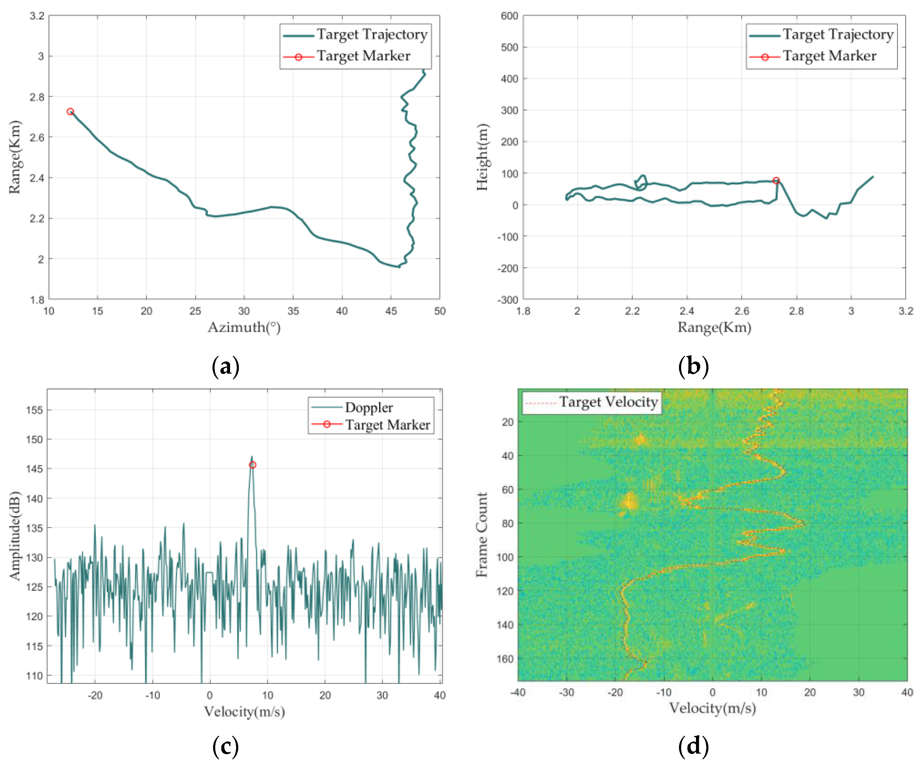
2.1. Feature Description

The target TD data from the Ubiquitous Radar include tracking information (such as velocity, range, height, etc.) and Doppler information (one-dimensional Doppler data) for all track points within the track. The one-dimensional Doppler data for all track points of each track compose the two-dimensional Doppler data. For TD data, an intuitive display can be achieved using TD maps. The TD map includes a Range–Azimuth graph, Range–Height graph, Doppler waveform graph, and Doppler spectrogram, as detailed in Figure 1.

In a Doppler waveform graph, the X-axis represents radial velocity, while the Y-axis represents Doppler amplitude. The X-axis value corresponding to the red circle is the velocity value of the current track point.

The one-dimensional Doppler data of all track points of each track form two-dimensional Doppler data, with RGB color mapping to create a Doppler spectrogram, where the X-axis represents target radial velocity, and the Y-axis represents the track point index, which can also be understood as frame numbers or time. The Doppler spectrogram uses the brightness of colors to indicate the magnitude of the amplitude value of the one-dimensional Doppler data at corresponding positions, with red dashed lines superimposed on the main spectrum connecting the velocity values in the tracking information of each track point.

This section mainly provides a detailed introduction to the composition of TD data using TD map, and the next section will discuss the main feature differences of different targets on the Doppler spectrogram.

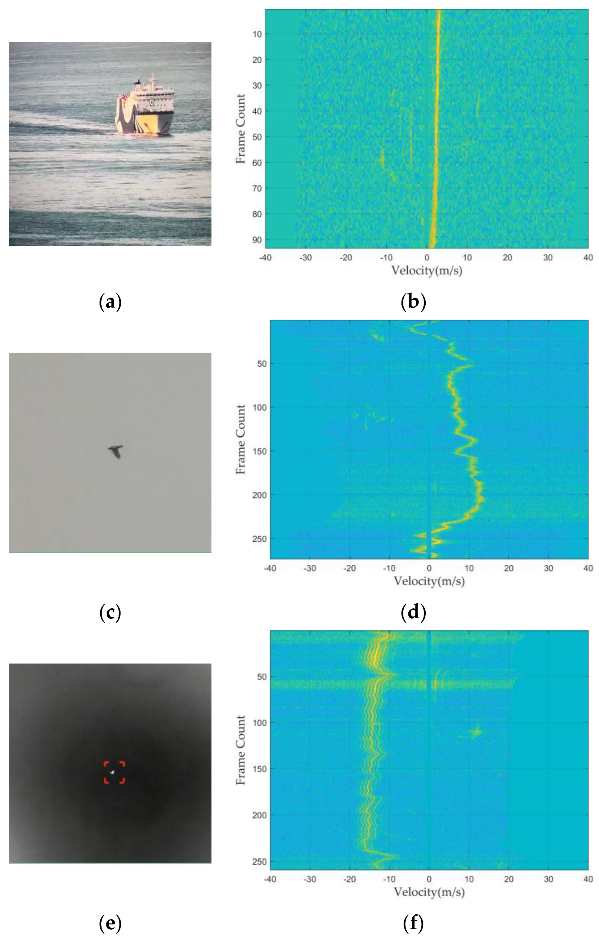
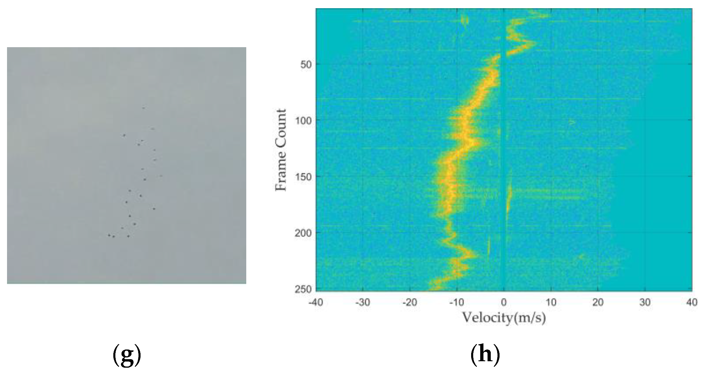
2.2. Doppler Signatures of Different Targets

Since the data type used for classification in this article is Doppler spectrograms, this section will first display the Doppler spectrograms of four types of targets: ships, birds, flapping birds, and bird flocks. On this basis, we will summarize the main differences in the spectral maps between these four types of targets.

The Ubiquitous Radar system consists of radar and optoelectronic components. After the radar completes the detection, tracking, and identification of targets, it guides the optoelectronic system to perform further integrated recognition of the targets. The Doppler spectrograms and optoelectronic images of the four types of targets are shown in the following figure.

Based on Figure 2, we can conclude that there are significant differences between the four types of targets, mainly in three aspects: maneuverability, the width of the main Doppler spectrum, and micro-motion characteristics. In terms of maneuverability, it is mainly reflected in the fluctuation amplitude of the main spectrum relative to the zero Doppler in the Doppler spectrogram, that is, the change in radial velocity. As can be seen from Figure 2, ships have lower maneuverability compared with other targets. Regarding the width of the Doppler main spectrum, the width of the main spectrum can well reflect the number of targets, with the spectrum width of group targets being wider than that of single targets. From Figure 2, it is observed that the Doppler width of bird flocks is larger than that of other targets. Micro-motion is generated by the rotating parts of the target and is manifested in the Doppler spectrogram as micro-motion spectra symmetrically distributed around the main spectrum [21]. The Ubiquitous Radar can display relatively obvious micro-motion characteristics for targets with high-speed wing flapping.

This section presents the Doppler spectrograms of the four types of targets and summarizes their different spectral characteristics. From the Doppler spectrograms, it is also evident that the main spectrum and its adjacent features are primarily used to identify the four types of targets, with information beyond this contributing little to target identification. The next section will elaborate on methods for enhancing the main spectrum and its adjacent features during the data preprocessing process.

3. Data Preprocessing

This section will elaborate in detail on the method of generating an Alpha layer using the velocity components in the tracking information and combining it with the original RGB three-channel Doppler spectrogram to form an RGBA four-channel Doppler spectrogram.

3.1. Radar Working Mode

The detection, tracking, and identification process of the Ubiquitous Radar is illustrated in the figure below.

Figure 3 shows that the Ubiquitous Radar belongs to the radar system that employs TTI technology. That is, it performs object identification after point-to-track correlation and track formation. The TTI working mode provides more abundant information for the identification module and can significantly enhance the recognizability of the targets [22].

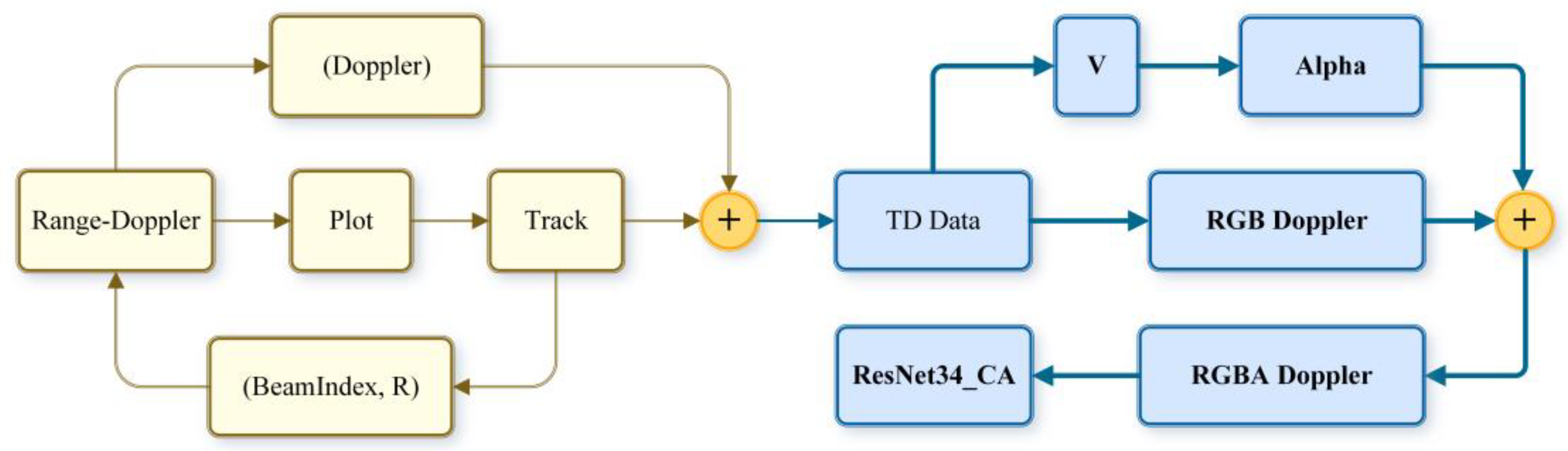
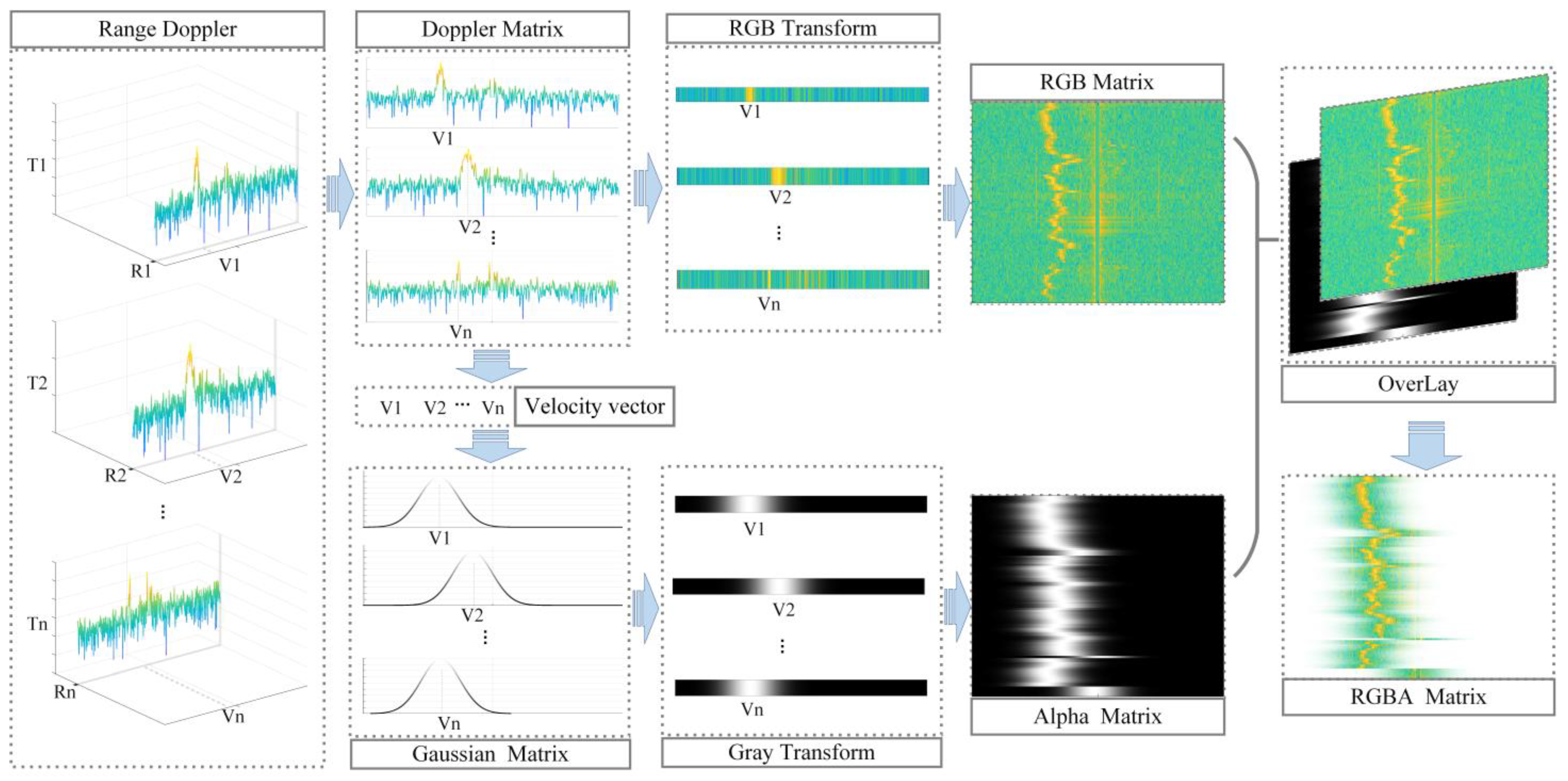
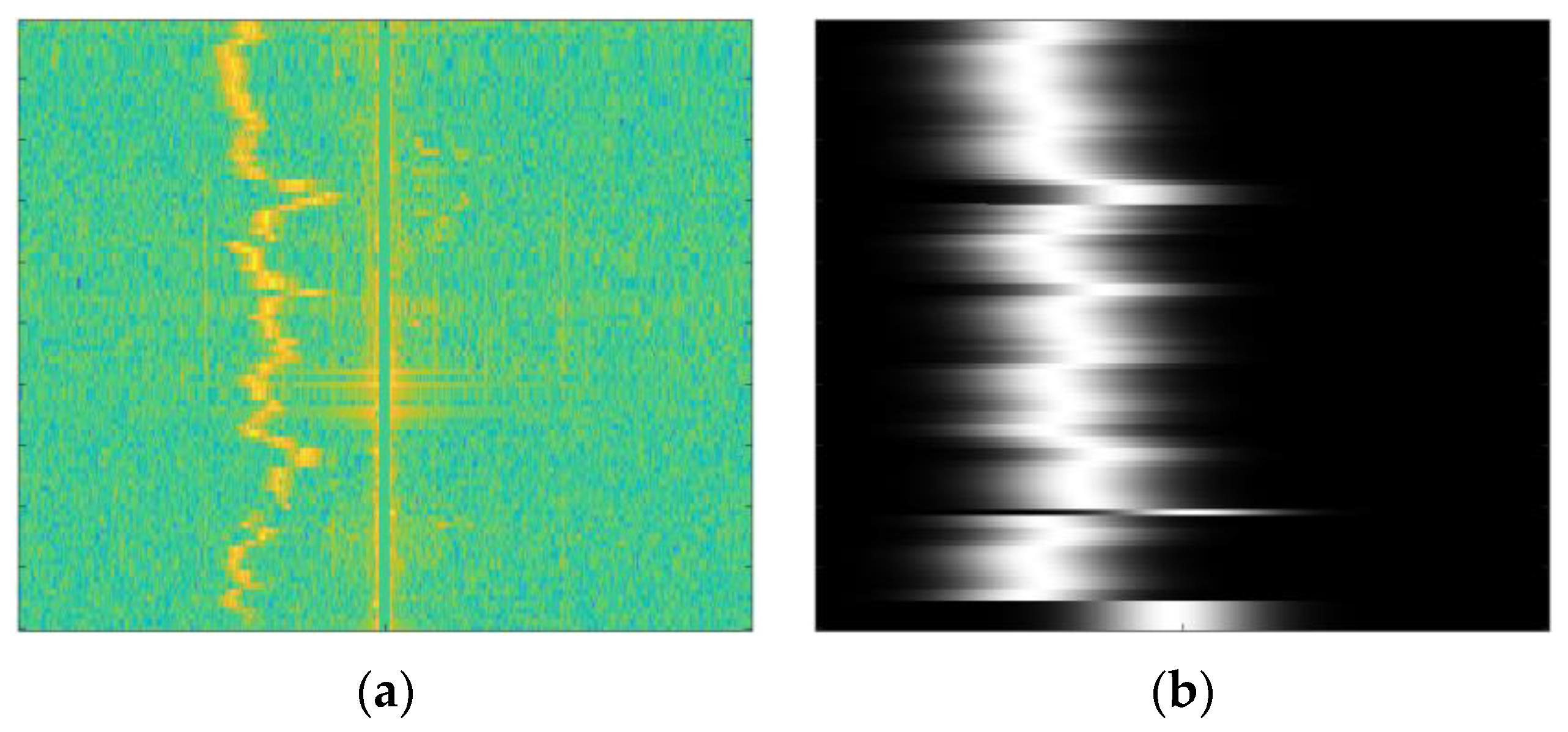
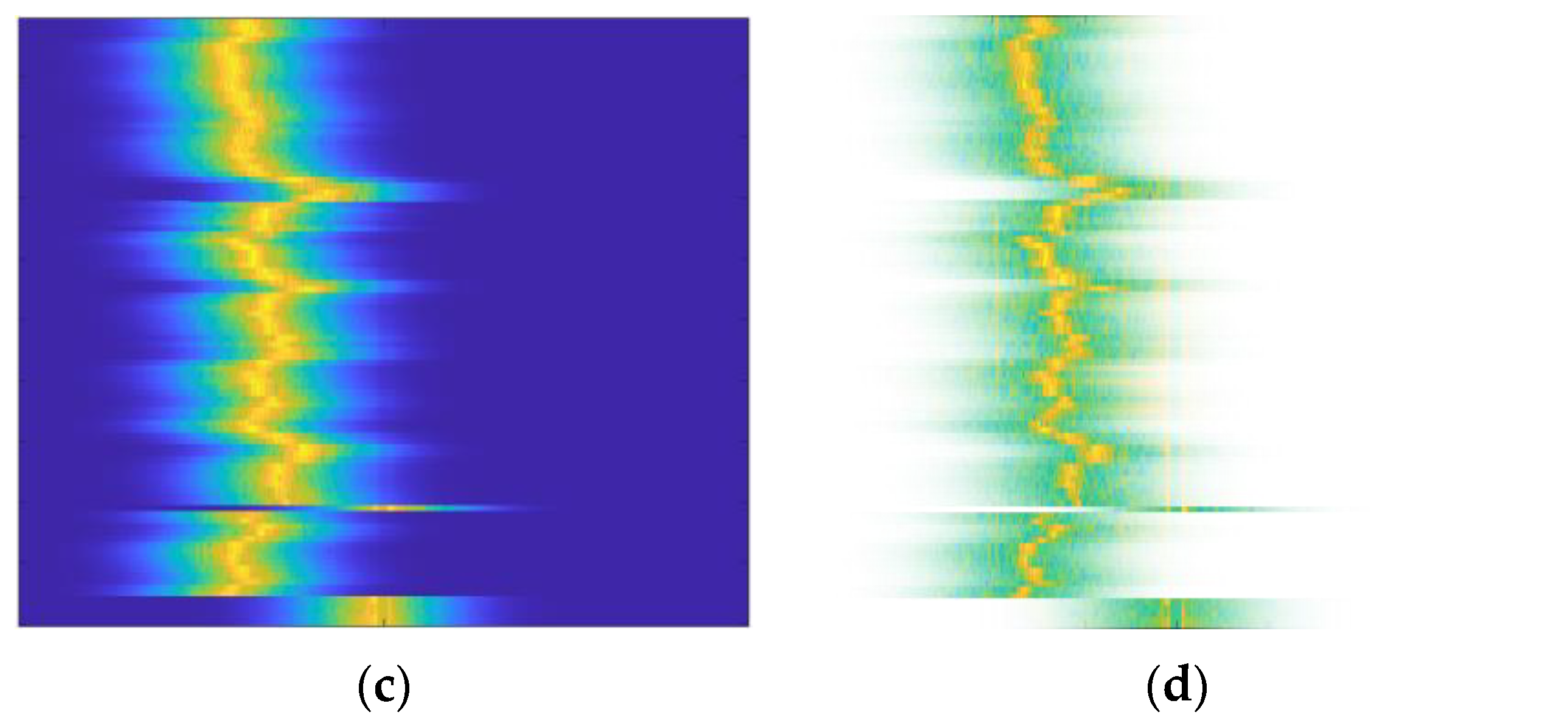
3.2. Steps for Generating RGBA Four-Channel Doppler Spectrogram

Based on this working mode, the Ubiquitous Radar provides track data for the identification module and also adds Doppler data. The Doppler data consist of one-dimensional data in the Doppler dimension obtained from range–Doppler (RD) data based on distance indexing within the tracking information. The one-dimensional Doppler data of all track points constitute two-dimensional Doppler data, which is then converted into RGB three-channel Doppler spectrograms using the RGB mapping matrix. The steps for generating an RGBA four-channel Doppler spectrogram using the feature enhancement layer are shown in the diagram below.

From Figure 4, it can be seen that to generate the RGBA four-channel spectrogram, the velocity elements from the tracking information are primarily used as the mean parameters of the Gaussian distribution. The Gaussian distribution row vectors of all track points form a two-dimensional Gaussian distribution matrix, which is the feature enhancement layer. Using gray mapping, the feature enhancement layer can be converted into the Alpha layer. This Alpha layer is then combined with the RGB three-channel Doppler spectrogram, generated using RGB mapping, to form the RGBA four-channel Doppler spectrogram. The inclusion of the Alpha layer, without altering the original RGB three-channel Doppler spectrogram, indicates the distribution area of the main features of the classification network [23].

3.3. Detailed Description of Generating RGBA Four-Channel Doppler Spectrogram

A Doppler matrix $\mathit{D}\in {ℝ}^{{\mathrm{N}}^{\mathrm{f}}\times {\mathrm{N}}^{\mathrm{d}}}$ is given, where ${\mathrm{N}}^{\mathrm{f}}$ is the number of frames, ${\mathrm{N}}^{\mathrm{d}}$ is the Doppler length, and the RGB color mapping matrix ${\mathit{C}}^{\mathrm{rgb}}\in {ℝ}^{{\mathrm{N}}^{\mathrm{rgb}}\times 3}$, where ${\mathrm{N}}^{\mathrm{rgb}}$ is the number of rows in the RGB color mapping matrix. In gray color mapping matrix ${\mathit{C}}^{\mathrm{gray}}\in {ℝ}^{{\mathrm{N}}^{\mathrm{gray}}}$, ${\mathrm{N}}^{\mathrm{gray}}$ is the number of rows in the gray color mapping matrix, and the velocity column vector is ${\mathit{V}}^{\mathrm{P}}\in {ℝ}^{{\mathrm{N}}^{\mathrm{f}}}$.

1.

Generation of Doppler Matrix:

This process normalizes the Doppler matrix $\mathit{D}$, composed of one-dimensional Doppler data corresponding to all track points, to form the Doppler matrix ${\mathit{D}}^{\mathrm{N}}$:

$${\mathit{D}}_{i,j}^{\mathrm{N}}={\displaystyle \frac{{\mathit{D}}_{i,j}-\min (\mathit{D})}{\max (\mathit{D})-\min (\mathit{D})}},\hspace{1em}1\le i\le {\mathrm{N}}^{\mathrm{f}}\hspace{1em}1\le j\le {\mathrm{N}}^{\mathrm{d}},$$

(1)

where ${\mathit{D}}^{\mathrm{N}}$ is the normalized Doppler matrix, $\min ()$ is the function to find the minimum value of the matrix, $\max ()$ is the function to find the maximum value of the matrix, $i$ is the row index of $\mathit{D}$ and ${\mathit{D}}^{\mathrm{N}}$, and $j$ is the column index of $\mathit{D}$ and ${\mathit{D}}^{\mathrm{N}}$.

2.

RGB Transform Process:

This process generates row indices for the RGB color mapping matrix based on the values in the Doppler matrix ${\mathit{D}}^{\mathrm{N}}$:

$$I_{i,j}^{\mathrm{rgb}}=round({\mathit{D}}_{i,j}^{\mathrm{N}}\ast {\mathrm{N}}^{\mathrm{rgb}}),\hspace{1em}1\le i\le {\mathrm{N}}^{\mathrm{f}}\hspace{1em}1\le j\le {\mathrm{N}}^{\mathrm{d}},$$

(2)

where $round()$ is defined as the adjacent rounding function, $I_{i,j}^{\mathrm{rgb}}$ is the row index in ${\mathit{C}}^{\mathrm{rgb}}$, which corresponds to ${\mathit{D}}_{i,j}^{\mathrm{N}}$, with $i$ being the row index of ${\mathit{D}}^{\mathrm{N}}$, and $j$ is the column index of ${\mathit{D}}^{\mathrm{N}}$

3.

Generation of RGB Matrix:

Based on the values in the Doppler matrix, use the color indices to generate a RGB three-channel Doppler matrix of the same size as the horizontal dimension of the Doppler matrix.

Create an RGB three-channel Doppler matrix ${\mathit{D}}^{\mathrm{rgb}}\in {ℝ}^{{\mathrm{N}}^{\mathrm{f}}\times {\mathrm{N}}^{\mathrm{d}}\times 3}$, and assign the RGB values from the ${\mathit{C}}^{\mathrm{rgb}}$ to it based on the index $I_{i,j}^{\mathrm{rgb}}$.

$${\mathit{D}}_{i,j,k}^{\mathrm{rgb}}={\mathit{C}}_{I_{i,j}^{\mathrm{rgb}},k}^{\mathrm{rgb}},\hspace{1em}1\le i\le {\mathrm{N}}^{\mathrm{f}}\hspace{1em}1\le j\le {\mathrm{N}}^{\mathrm{d}}\hspace{1em}k\in \{1,2,3\}\hspace{1em}1\le I_{i,j}^{\mathrm{rgb}}\le {\mathrm{N}}^{\mathrm{rgb}},$$

(3)

where $i$ is the row index of the ${\mathit{D}}^{\mathrm{rgb}}$, $j$ is the column index of the ${\mathit{D}}^{\mathrm{rgb}}$, and $k$ is the column index of the ${\mathit{C}}^{\mathrm{rgb}}$, as well as the channel index of the ${\mathit{D}}^{\mathrm{rgb}}$.

4.

Generation of Gaussian Matrix:

Since the position of each track point’s one-dimensional Doppler data main spectrum corresponds to the target’s radial velocity, a characteristic enhancement matrix indicating the main spectrum area can be generated using the radial velocity values of all track points. After normalization, this forms the Gaussian matrix.

• (a)

  Let the Gaussian distribution matrix be $\mathit{A}\in {ℝ}^{{\mathrm{N}}^{\mathrm{f}}\times {\mathrm{N}}^{\mathrm{d}}}$, where ${\mathrm{N}}^{\mathrm{f}}$ is the number of frames and ${\mathrm{N}}^{\mathrm{d}}$ is the Doppler length. Given the gray color mapping vector ${\mathit{C}}^{\mathrm{gray}}\in {ℝ}^{{\mathrm{N}}^{\mathrm{gray}}}$, with ${\mathrm{N}}^{\mathrm{gray}}$ representing the number of rows in the gray color mapping vector, and the speed column vector being ${\mathit{V}}^{\mathrm{P}}\in {ℝ}^{{\mathrm{N}}^{\mathrm{f}}}$, generate the Gaussian distribution matrix:

  $${\mathit{A}}_i=\mathcal{N}\left({\mathit{V}}_i^{\mathrm{p}}, {\sigma }^2\right),$$

  (4)

  where $\mathcal{N}\left({\mathit{V}}_i^{\mathrm{p}}, {\sigma }^2\right)$ represents a normal distribution, with a mean of ${\mathit{V}}_i^{\mathrm{P}}$ and a standard deviation of $\sigma$, generating a vector of length ${\mathrm{N}}^{\mathrm{d}}$, and $i$ is the row index of ${\mathit{V}}^{\mathrm{P}}$ as the row index of the $\mathit{A}$.

  (b)

  Normalize the $\mathit{A}$ to form ${\mathit{A}}^{\mathrm{N}}$:

  $${\mathit{A}}_{i,j}^{\mathrm{N}}={\displaystyle \frac{{\mathit{A}}_{i,j}-\min (\mathit{A})}{\max (\mathit{A})-\min (\mathit{A})}},\hspace{1em}1\le i\le {\mathrm{N}}^{\mathrm{f}}\hspace{1em}1\le j\le {\mathrm{N}}^{\mathrm{d}}$$

  (5)

  where ${\mathit{A}}^{\mathrm{N}}$ is the normalized Gaussian distribution matrix, $\min ()$ is the function to find the minimum value of the matrix, $\max ()$ is the function to find the maximum value of the matrix, $i$ is the row index of $\mathit{A}$ and ${\mathit{A}}^{\mathrm{N}}$, and $j$ is the column index of $\mathit{A}$ and ${\mathit{A}}^{\mathrm{N}}$.

5.

Gray Transform Process:

Generate row indices for the gray color mapping vector based on the values in the Gaussian matrix:

$$I_{i,j}^{\mathrm{gray}}=round({\mathit{A}}_{i,j}^{\mathrm{N}}\ast {\mathrm{N}}^{\mathrm{gray}}),\hspace{1em}1\le i\le {\mathrm{N}}^{\mathrm{f}}\hspace{1em}1\le j\le {\mathrm{N}}^{\mathrm{d}},$$

(6)

where $round()$ is defined as the adjacent rounding function, $I_{i,j}^{\mathrm{gray}}$ is the row index in ${\mathit{C}}^{\mathrm{gray}}$, which corresponds to the ${\mathit{A}}_{i,j}^{\mathrm{N}}$, $i$ is the row index of ${\mathit{A}}^{\mathrm{N}}$, and $j$ is the column index of ${\mathit{A}}^{\mathrm{N}}$.

6.

Generation of Alpha Matrix:

Generate an Alpha layer matrix of the same size as the Gaussian matrix based on the color indices corresponding to the values in the Gaussian matrix.

Set the Alpha layer matrix as ${\mathit{D}}^{\mathrm{alpha}}\in {ℝ}^{{\mathrm{N}}^{\mathrm{f}}\times {\mathrm{N}}^{\mathrm{d}}}$, and assign the corresponding values from ${\mathit{C}}^{\mathrm{gray}}$ to the according to the index $I^{\mathrm{gray}}$.

$${\mathit{D}}_{i,j}^{\mathrm{alpha}}={\mathit{C}}_{I_{i,j}^{\mathrm{gray}}}^{\mathrm{gray}},\hspace{1em}1\le i\le {\mathrm{N}}^{\mathrm{f}}\hspace{1em}1\le j\le {\mathrm{N}}^{\mathrm{d}}\hspace{1em}1\le I_{i,j}^{\mathrm{gray}}\le {\mathrm{N}}^{\mathrm{gray}},$$

(7)

where $i$ is the row index of ${\mathit{D}}^{\mathrm{alpha}}$, $j$ is the column index of ${\mathit{D}}^{\mathrm{alpha}}$, and $I_{i,j}^{\mathrm{gray}}$ is the row index in ${\mathit{C}}^{\mathrm{gray}}$ that corresponds to the ${\mathit{A}}_{i,j}^{\mathrm{N}}$.

7.

Generation of RGBA Matrix:

Merge the Doppler matrix and the Alpha layer matrix along the channel dimension.

Merge the RGB matrix from (3) with the Alpha matrix from (7) to form the RGBA four-channel matrix ${\mathit{D}}^{\mathrm{rgba}}\in {ℝ}^{{\mathrm{N}}^{\mathrm{f}}\times {\mathrm{N}}^{\mathrm{d}}\times 4}$.

$$\left\{\begin{array}{cc}{\mathit{D}}_{i,j,k}^{\mathrm{rgb}}\hfill & k\in \left\{1,2,3\right\}\\ {\mathit{D}}_{i,j}^{\mathrm{alpha}}\hfill & k=4\end{array}\right.,$$

(8)

where $i$ is the row index of the ${\mathit{D}}^{\mathrm{alpha}}$ and ${\mathit{D}}^{\mathrm{rgb}}$ matrices, $j$ is the column index of the ${\mathit{D}}^{\mathrm{alpha}}$ and ${\mathit{D}}^{\mathrm{rgb}}$ matrices, and $k$ is the color channel index. The values of the three channels of the ${\mathit{D}}^{\mathrm{rgb}}$ matrix are assigned to the first three channels (i.e., R, G, and B channels) of the ${\mathit{D}}^{\mathrm{rgba}}$ matrix, and the values of the ${\mathit{D}}^{\mathrm{alpha}}$ matrix are assigned to the fourth channel (i.e., Alpha channel) of the ${\mathit{D}}^{\mathrm{rgba}}$ matrix. This completes the image preprocessing. This section first introduces the work mode of Ubiquitous Radar, which is TTI. This mode provides more target information for the identification module, adding Doppler data to the existing track data. Based on this work mode, we designed a spectrogram local enhancement method that uses tracking information to generate a transparent layer, which is combined with the original RGB three-channel Doppler spectrogram to form an RGBA four-channel spectrogram. This method of spectrogram local enhancement amplifies the main spectrum and its adjacent features while attenuating features outside of this area.

The addition of the Alpha layer highlights specific areas in the spectrogram, and the extra information can help the network learn useful features more quickly, thus accelerating the convergence speed and enhancing the model’s generalization ability. The next section will detail the design of the neural network classifier.

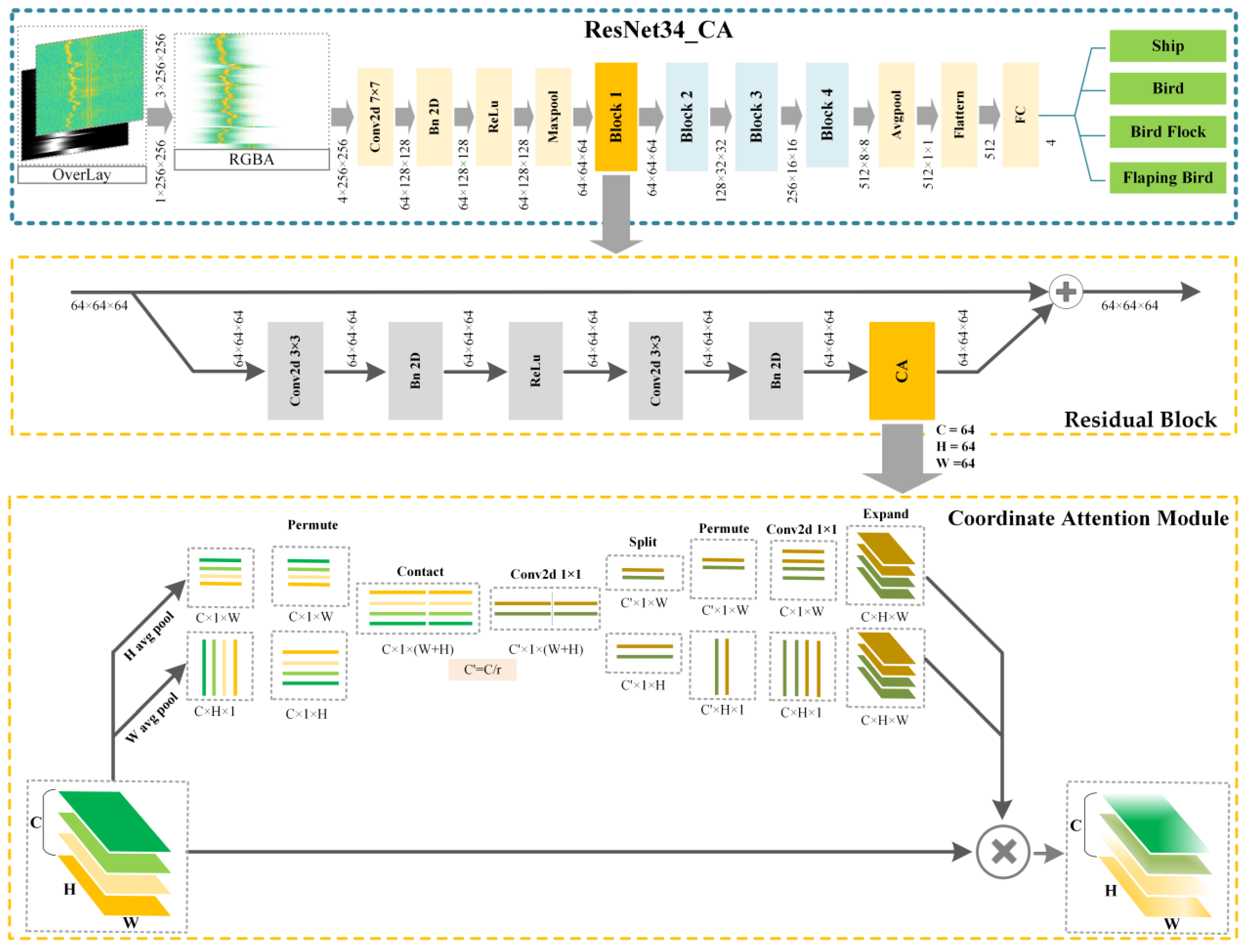
4. Classifier Design

In the previous two sections, we gained a comprehensive understanding of the data composition of the Ubiquitous Radar, the Doppler spectrograms of different targets and their distinctions, and the data preprocessing process. This section will provide a detailed introduction to the classifier design, as illustrated in the following figure.

Figure 5 is primarily composed of three parts: the overall network architecture, the residual module architecture, and the attention module architecture.

Firstly, the overall network architecture includes several key components. The input layer consists of a four-channel RGBA Doppler spectrogram. This is followed by convolutional and pooling layers where features are extracted through a series of convolution operations, including 7 × 7 convolutions, and pooling operations such as max pooling. Next, the architecture incorporates residual modules composed of multiple residual blocks, each integrated with a CA module to enhance feature representation [24]. Finally, the classification layer uses fully connected layers to classify the extracted features, producing outputs that include four categories: ship, bird, bird flock, and flapping bird.

Secondly, the residual module architecture contains several critical elements. Each residual block includes two 3 × 3 convolutional kernels that further extract input features. Following each convolutional layer, batch normalization and the ReLU activation function are applied to standardize inputs and introduce non-linearity, which helps accelerate the training process and improve the model’s representational capacity. The architecture also features a skip connection that directly adds the input features to the output features, preserving the original information and mitigating the gradient vanishing problem, leading to more stable training. Additionally, each residual block is integrated with a CA module to further enhance feature representation through the coordinate attention mechanism.

Thirdly, the CA module architecture includes several key components. First, spatial information encoding involves performing global average pooling operations in the height (H) and width (W) directions to generate two one-dimensional feature vectors representing global features in these directions. These feature vectors are then transposed and concatenated to form a combined feature vector. Next, channel interaction processes the combined feature vector through a 1 × 1 convolution layer and a batch normalization layer, followed by a ReLU activation function to generate an intermediate feature vector. This intermediate feature vector is then split into two parts, corresponding to the height and width directions. Finally, the remapping operation passes the split feature vectors through separate 1 × 1 convolution layers to generate attention weight vectors for the height and width directions. These weight vectors are normalized using the sigmoid function to obtain the final attention map. The attention map is then expanded back to the size of the input feature map and multiplied element-wise with the input feature map, enabling the network to focus more on important spatial locations and features.

Through this well-designed network, several improvements are achieved. Firstly, the CA attention module, unlike channel attention, converts the feature tensor into a single feature vector via 2D global pooling [25] and encodes and decodes spatial information, introducing the coordinate attention mechanism. This allows the network to better capture spatial features of targets, improving classification accuracy, particularly in complex scenes. Additionally, the skip connection mechanism in residual modules alleviates the gradient vanishing problem in deep networks, making training more stable and efficient, which is crucial for deep learning tasks [26].

5. Results and Discussion

5.1. Experimental Environment

5.1.1. Radar System Parameters

The field setup and main parameters of the Ubiquitous Radar are shown in Figure 6. This setup illustrates the installation positions and configurations of the radar and electro-optical equipment, ensuring optimal detection performance within the monitoring area. Specific parameters include the radar’s operating frequency, bandwidth, pulse repetition frequency, update rate, detection range, and the electro-optical equipment’s scanning method, scanning time, output method, frame rate, and detection range. These parameters provide the foundation for the system’s efficient operation.

The radar equipment uses a wide-beam transmitting antenna that can cover a 90° azimuth sector centered on the antenna’s line of sight [27,28]. The receiving antenna is composed of multiple grid-structured sensors. When receiving echo data, digital beamforming technology is used to form multiple receiving beams [29,30], covering the entire monitoring scene. The optoelectronic equipment can receive guidance from the radar equipment to detect and track targets. Together, they can quickly and effectively detect, provide early warning for, and document LSS targets in the airport’s clearance zone.

5.1.2. Computer Specifications

The computer used for training the network was equipped with an Intel i7-13700KF CPU, 32 GB of memory running at 4400 MHz, and 1 TB of storage. It featured an NVIDIA GeForce RTX 4090D GPU. The development environment included PyCharm version 2023.3.6 as the integrated development environment (IDE), PyTorch version 2.2.1 for the deep learning library, and CUDA version 11.8.

5.2. Dataset Composition

The dataset used in this paper primarily contains four types of targets: ships, birds, flapping birds, and bird flocks. The composition of the dataset is shown in

Table 1. Dataset composition.

Type	Training Set	Test Set	Total	Category Index
Ship	824	250	1074	1
Bird	1121	328	1449	2
Flapping bird	1090	306	1396	3
Bird flock	705	266	971	4

.

Figure 7 shows the RGB three-channel Doppler spectrograms for the four target types.

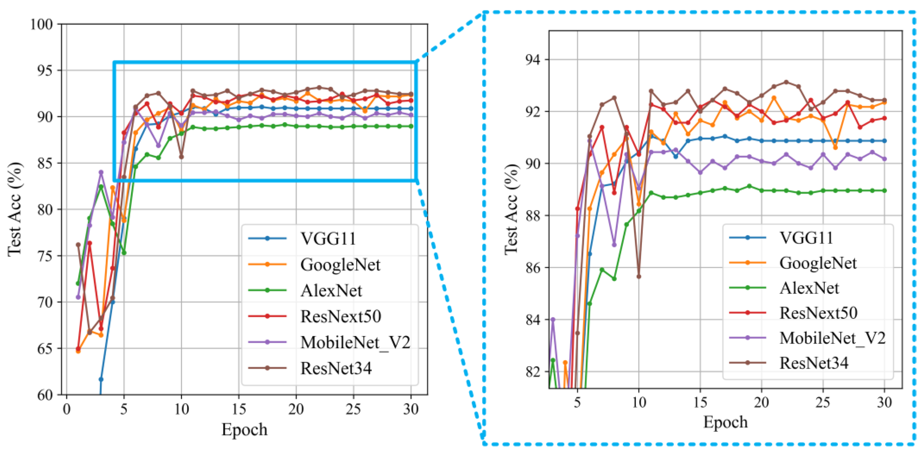
5.3. Selection of Classification Backbone Networks

In this section, the original RGB three-channel Doppler spectrogram is used as network input to test the classification accuracy of six networks: VGG11 [31], GoogleNet [32], AlexNet [33], ResNext50 [34], MobileNet_V2 [35], and ResNet34, as shown in Figure 8 and

Table 2. Comparison graph of different classifiers.

Type	Precision (%)	Recall (%)	F1_Score (%)	Accuracy (%)
VGG11	91.54	91.34	91.4	91.04
GoogleNet	93.06	92.69	92.85	92.52
AlexNet	89.79	89.61	89.65	89.13
ResNext50	92.86	92.71	92.77	92.43
MobileNet_V2	91.86	91	91.3	90.87
ResNet34	93.52	93.35	93.42	93.13

. The optimal backbone network is then selected.

From Figure 8 and Table 2, it is evident that ResNet34 demonstrates significant performance advantages compared with other networks. After stabilization, ResNet34 achieved an accuracy of 93.13%, which is noticeably higher than the performance of other networks. This result indicates that ResNet34 not only adapts to data more quickly but also maintains high classification accuracy after extended training periods, showcasing its strong potential and reliability in practical applications.

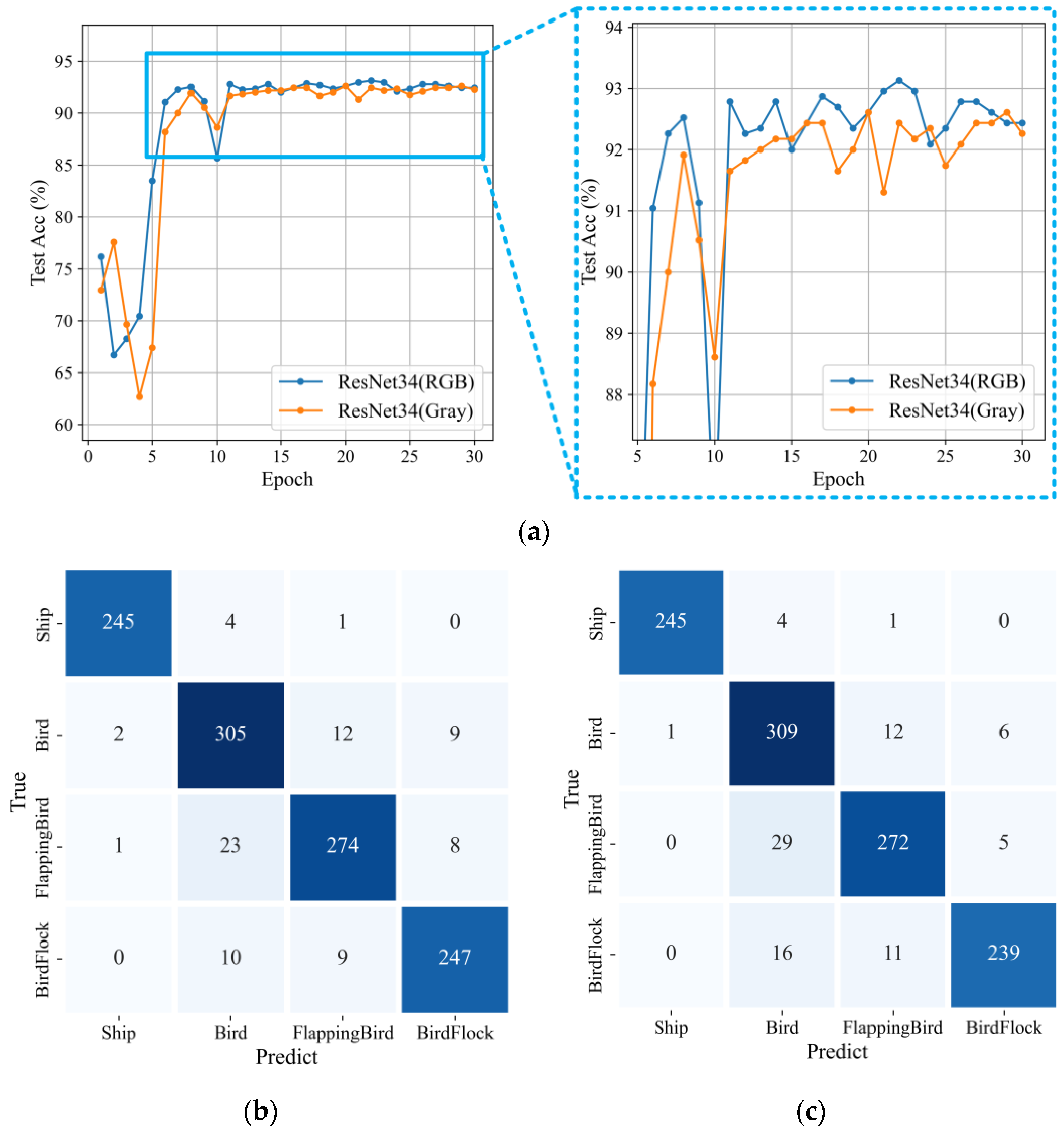
5.4. Selection of Classification Data Sources

From the comparative experiments in the previous section, it can be seen that the classification effect of ResNet34 is significantly better than the other five types of networks. This section will compare the classification results of RGB three-channel Doppler spectrograms and gray single-channel Doppler spectrograms based on ResNet34, as shown in Figure 9 and

Table 3. Classification comparison chart of different data sources.

Type	Precision (%)	Recall (%)	F1_Score (%)	Accuracy (%)
RGB	93.52	93.35	93.42	93.13
Gray	93.35	92.74	92.97	92.61

.

From Figure 9 and Table 3, it is evident that regarding accuracy comparison, the classification accuracy of RGB three-channel Doppler spectrograms increased from 92.61% to 93.13% compared with gray single-channel Doppler spectrograms. In the comparison of the confusion matrix, the confusion matrix of the gray single-channel Doppler spectrogram increased errors mainly in two aspects: birds and flapping birds and birds and bird flocks compared with the RGB three-channel Doppler spectrogram, indicating that the grayscale image has reduced the amount of information in the spectrograms to some extent, weakening the features of the main spectral width and micro-motion. Compared with this, RGB images can retain more information, especially color information. Therefore, for the fine classification work of similar targets that need to utilize the bandwidth of the main spectrum, especially the micro-motion features, RGB images as the data source for classification are undoubtedly the best choice.

Integrating the above experimental comparisons and the advantages of RGB images, this study used RGB three-channel Doppler spectrograms as the basis. It employed the feature enhancement layer generated using tracking information as the Alpha layer. Finally, the two were merged to create an RGBA four-channel Doppler spectrogram as the data source for Ubiquitous Radar target classification.

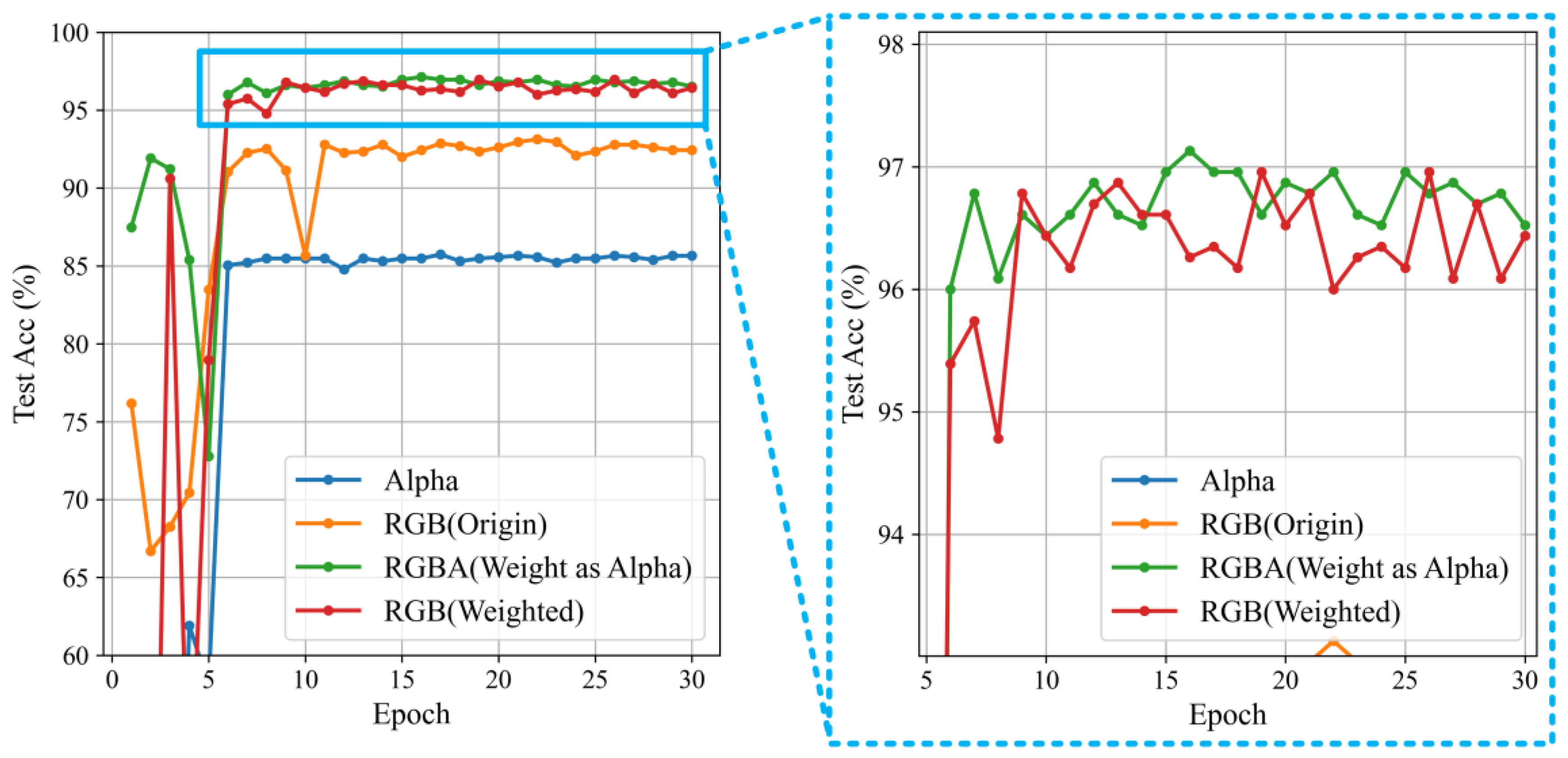
5.5. Selection of Feature Enhancement Methods

This section uses the ResNet34 backbone network to compare the classification effects of four types of data sources: the original RGB three-channel Doppler spectrograms, Alpha grayscale images, RGB three-channel Doppler spectrograms with a merged feature enhancement layer, and RGBA four-channel Doppler spectrograms with an overlaid feature enhancement layer. The RGB three-channel Doppler spectrograms with a merged feature enhancement layer are created by directly multiplying the feature enhancement layer with the original two-dimensional Doppler data and then transforming it using an RGB mapping matrix. The four types of input data are labeled in sequence as RGB (Origin), Alpha, RGB (Weighted), and RGBA (Weight as Alpha), with their data composition illustrated in Figure 10.

The classification results of the above four types of input data are shown in the following figure.

Firstly, by comparing the two processing methods of the feature enhancement layer, it can be seen from the classification results in Figure 11 and

Table 4. Classification comparison chart of different feature enhancement methods.

Type	Precision (%)	Recall (%)	F1_Score (%)	Accuracy (%)
Alpha	86.79	84.91	85.04	85.39
RGBA (Origin)	93.52	93.35	93.42	93.13
RGBA (Weight as Alpha)	97.21	97.16	97.18	97.13
RGBA (Weighted)	97.12	96.91	97.01	96.96

that the RGBA (Weight as Alpha) has a more advantageous result compared with the RGB (Weighted).

Secondly, to intuitively see the improvement in classification accuracy due to the addition of the feature enhancement layer, the following figure shows the difference in classification accuracy between RGBA (Weight as Alpha) and RGB (Origin).

From Figure 12, it can be seen that the addition of the feature enhancement layer significantly improves the classification effect. After the model converges, the stable accuracy increases by up to nearly 5%. The optimal accuracy improvement is 4%.

Finally, by comparing the confusion matrices of the three types of data—Alpha, RGB (Origin), and RGBA (Weight as Alpha)—we can summarize the improvement in classification effects brought about by the addition of the feature enhancement layer.

From Figure 13, it is clear that in terms of accuracy, the classification results of the RGBA (Weight as Alpha) images as network input remain the most advantageous. By comparing the confusion matrices of RGBA (Weight as Alpha) and RGB (Origin), the addition of the Alpha layer significantly reduces classification errors between flapping birds and birds and between flapping birds and bird flocks, further proving the Alpha layer’s substantial enhancement effect on the primary spectral features. Using the Alpha layer as network input, where only the maneuverability feature exists in the spectrum, compared with the classification results when RGB (Origin) is used as network input, the removal of primary spectral features, including spectral width and micro-motion characteristics, leads to a sharp decline in the classification effectiveness between birds and bird flocks. It is worth noting that the classification effect of flapping birds remains good when using the Alpha layer as network input because birds flapping their wings at high speeds have lower maneuverability compared with those flying at lower speeds but higher than that of smoothly sailing ships, which can also be inferred from the dataset thumbnails. If the differences in maneuverability of flapping birds are disregarded and only the Alpha layer is used as network input, the classification performance for the three categories—birds, bird flocks, and flapping birds—would drastically decrease.

The above experiments can be summarized as follows: using primary spectral characteristics can effectively classify sub-categories within the broad category of birds. The addition of a feature enhancement layer emphasizes the primary spectral features, further improving the classification performance.

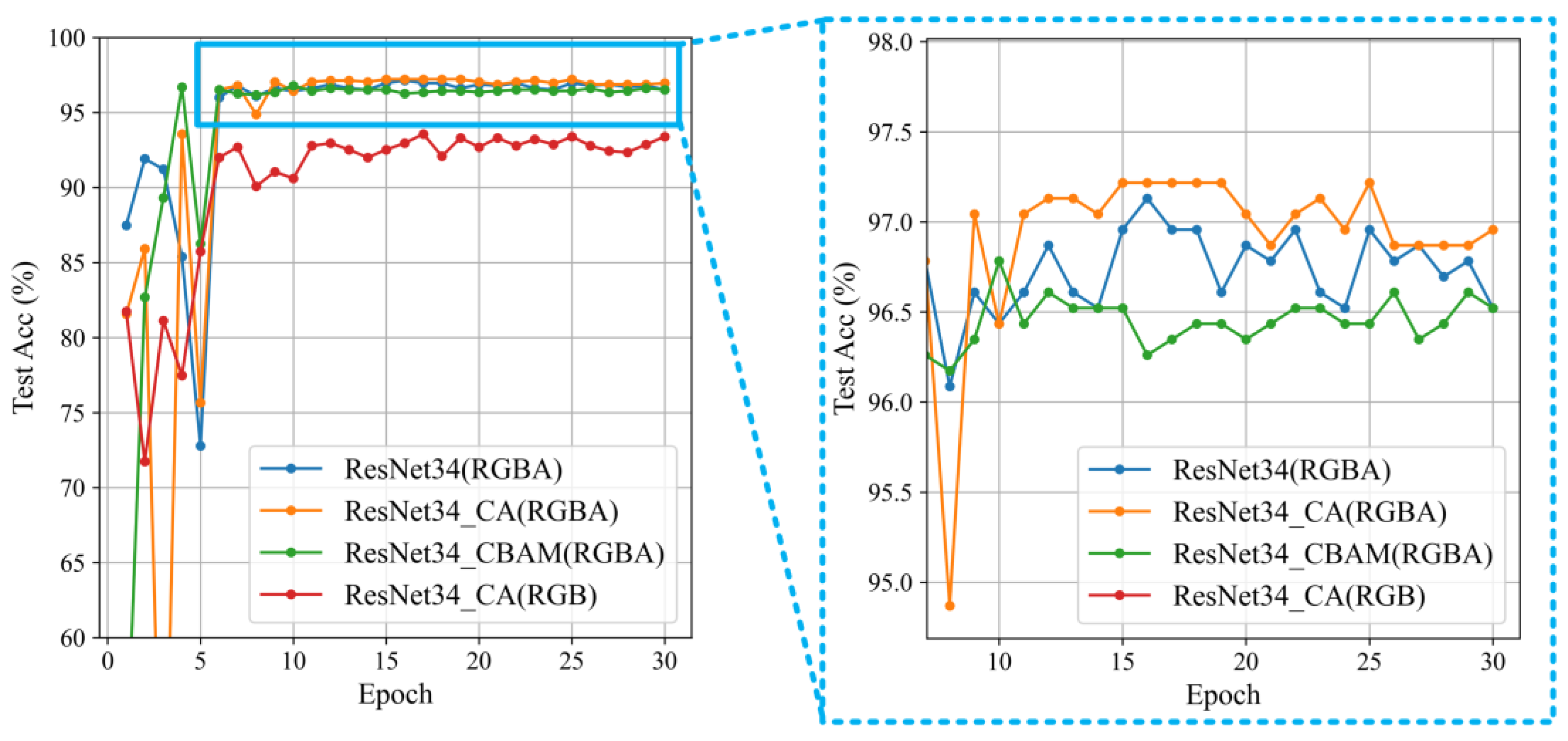
5.6. Attention Module Classification Accuracy Comparison

Building on the comparison of RGBA four-channel Doppler spectrograms classification using the ResNet34 backbone network in the previous section, this section integrates the CA module into the residual blocks of ResNet34, forming the ResNet34_CA network. Simultaneously, the convolutional block attention module (CBAM) [36] is incorporated into ResNet34 in the same manner, resulting in the ResNet34_CBAM network. This section uses RGBA four-channel Doppler spectrograms as the network input to compare the classification effects.

As can be seen from Figure 14 and

Table 5. Comparison graph of attention classification.

Type	Precision (%)	Recall (%)	F1_Score (%)	Accuracy (%)
Resnet34 (RGBA)	97.21	97.16	97.18	97.13
Resnet34_CA (RGBA)	97.41	97.15	97.26	97.22
Resnet34_CBAM (RGBA)	96.97	96.72	96.83	96.78
Resnet34_CA (RGB)	94.05	93.76	93.86	93.57

, the addition of the CA module has further improved the classification results of the network, with the accuracy increasing from 97.13% to 97.22%. This indicates that the integration of the CA attention module has made the network pay more attention to the main spectral information, thereby further improving the classification accuracy.

It is worth noting that this section also tested the input of RGB three-channel Doppler spectrograms into the ResNet34_CA network with an accuracy of 93.57%. Compared with the classification result of 93.13% for the ResNet34 network under the same input conditions, the improvement in classification performance brought about by the CA module is not as obvious as the improvement brought about by the addition of the Alpha layer.

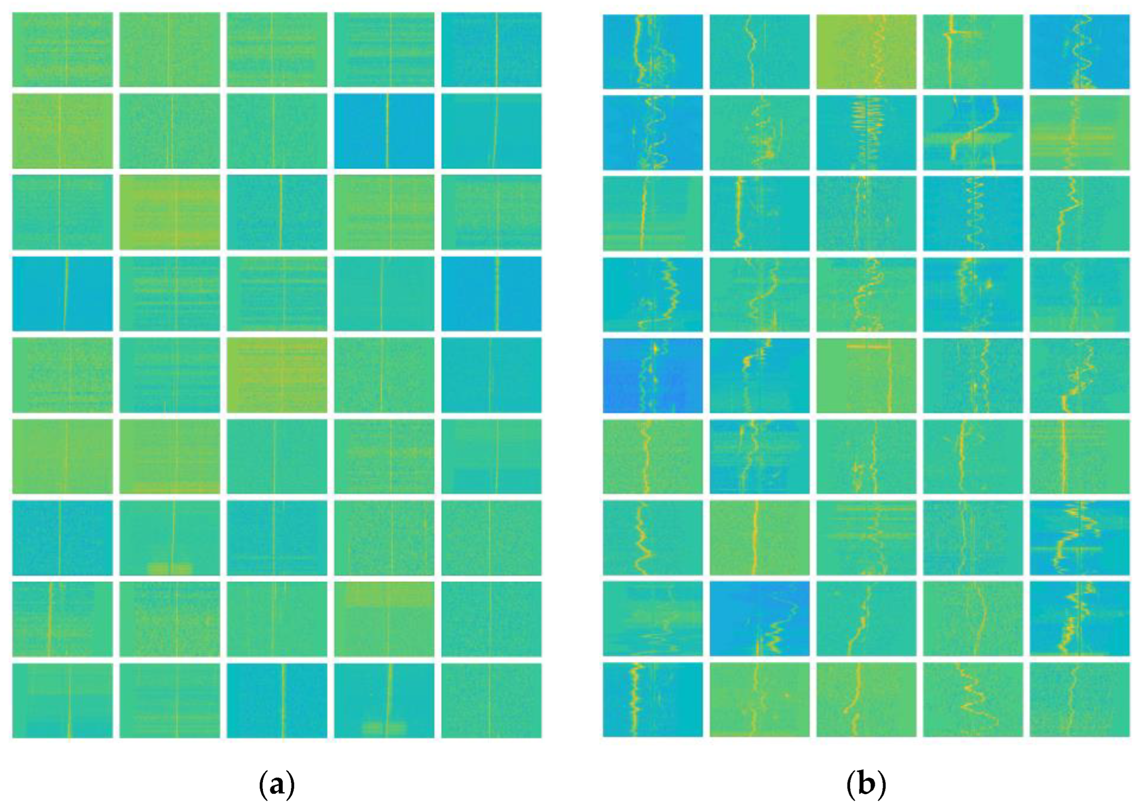
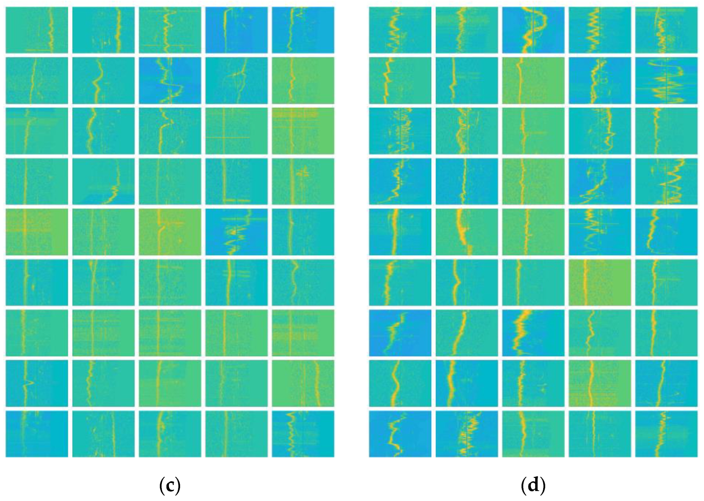
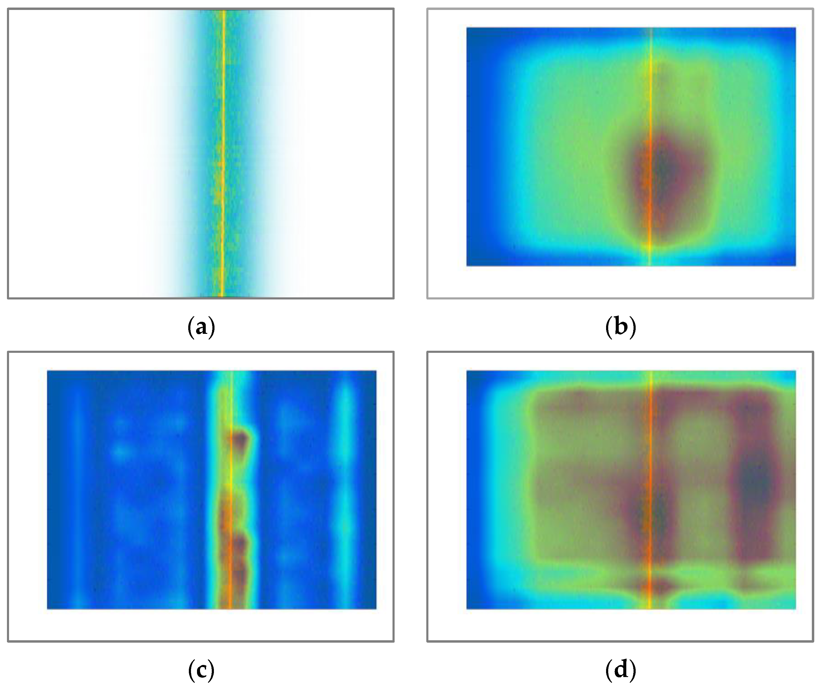
5.7. Comparative Analysis of CAM Visualizations

Based on the comparison of classification accuracies using different attention modules from the previous section, this section utilized RGBA four-channel Doppler spectrograms of ships as input. It employed Pytorch to load model parameters that achieve the highest accuracy on the test set during the classifier’s training process. A post hoc visualization explanation method based on CAM, Score-Cam, was used, and the last convolution layers of ResNet34, ResNet34_CA, and ResNet34_CBAM networks were input into the Score-Cam [37] module. The CAMs of these three networks are displayed respectively.

From Figure 15, it can be seen that, compared with other networks, the ResNet34_CA network can better focus attention on the main spectrum. Notably, the attention of the ResNet34_CBAM network is not as focused as that of ResNet34, which is also evident from the accuracy comparison in the previous section, with the classification accuracy of ResNet34_CBAM being lower than that of ResNet34 throughout the entire training process.

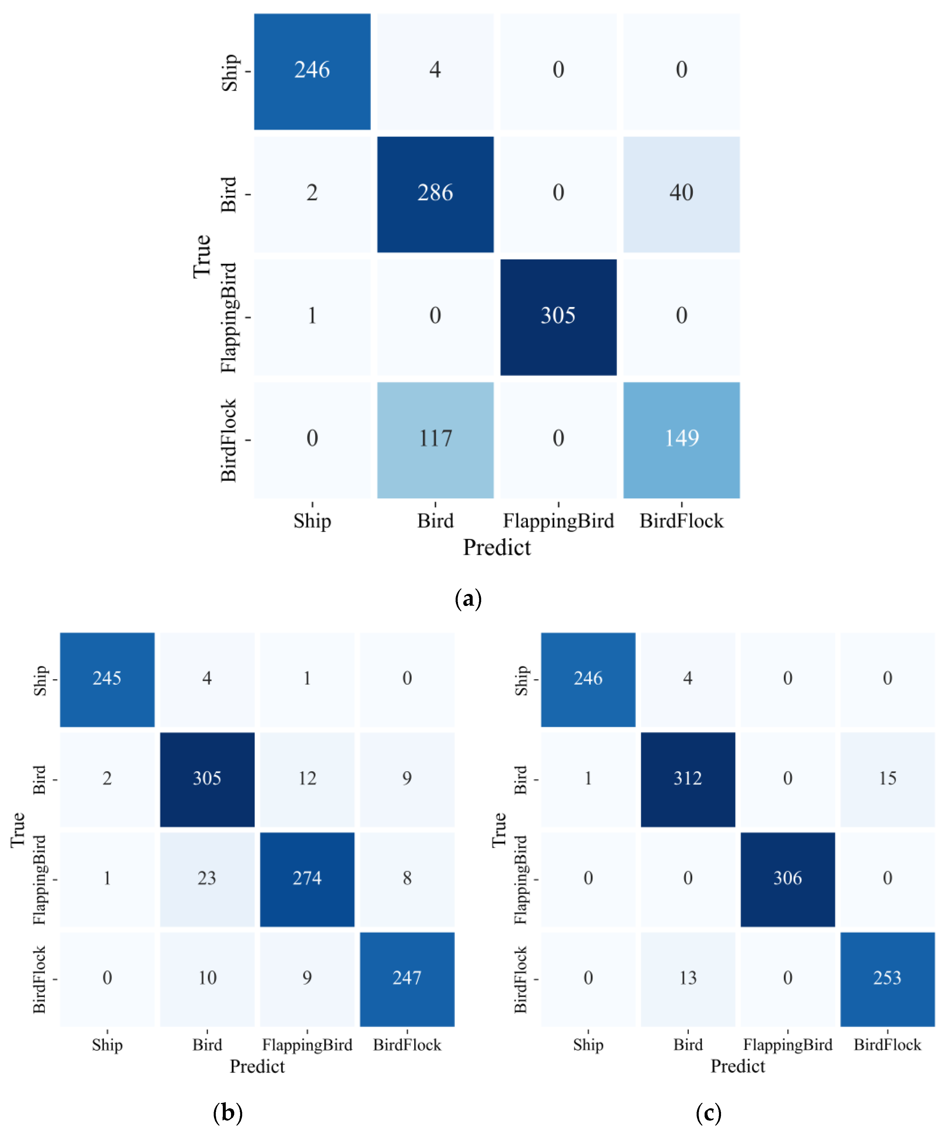
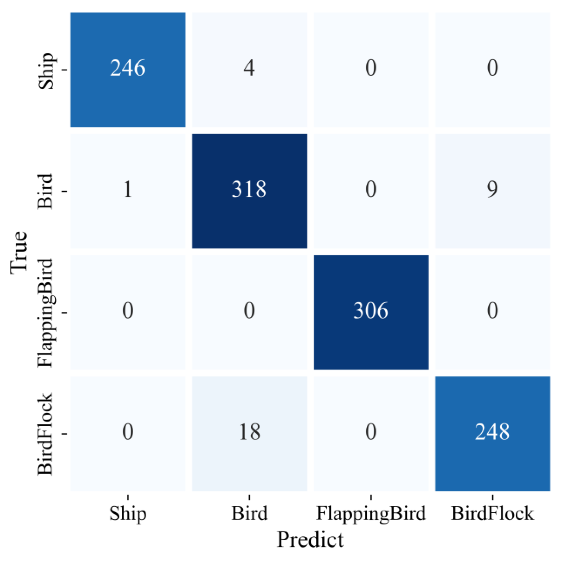
5.8. Confusion Matrix for Classification Results

From the comparisons in the two sections above, it is evident that the neural network structure of ResNet34_CA has more advantages. This section employed this structure, firstly utilizing the ‘confusion_matrix’ package from ‘sklearn’ and then using ‘seaborn’ to generate and display the confusion matrices for test sets. The results are shown in the figure below.

From Figure 16, it can be seen that the misclassification in testing sets is mainly concentrated between birds and bird flocks. Additionally, the classification accuracy of different targets varies. Firstly, whether using RGB three-channel Doppler spectrograms or RGBA four-channel Doppler spectrograms on ResNet34 or using RGBA four-channel Doppler spectrograms on ResNet34_CA, the classification performance of ships remains stable. This stability is due to two advantages of ships: first, ships have distinct differences in maneuverability, primary spectrum amplitude, and width compared with birds; second, the stability of these parameters over time is much stronger for ships than for birds. Among the three bird categories, the number of classification errors between birds and bird flocks is the most significant, while the classification accuracy for flapping birds is noticeably better than for the other two categories. This is because flapping birds have distinct micro-Doppler signatures that, when captured by the network, can effectively distinguish them from the other two bird categories. The errors in classifying birds and bird flocks can be attributed to several factors: first, the radar reflection intensity of birds and bird flocks may be similar, especially at greater radar distances. Secondly, the limited spatial resolution of the radar may prevent it from accurately distinguishing multiple closely spaced targets. Finally, the overall movement patterns of birds and bird flocks may be very similar, particularly in terms of maneuverability.

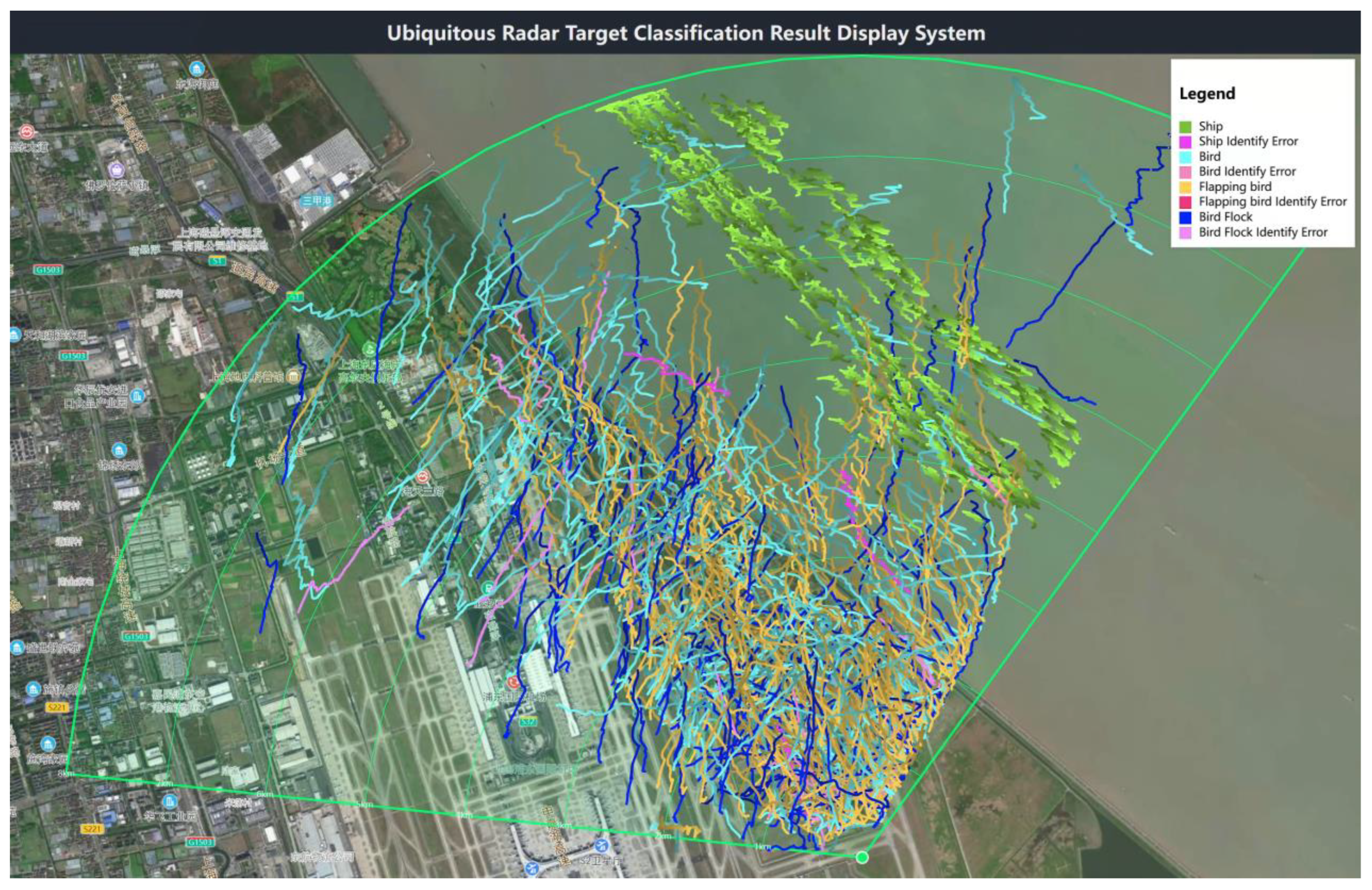
5.9. Map Display of Classification Results

Finally, the Amap API and Python were used to parse the flight tracks of targets in the test set into map path data and embed them into a static HTML page for visualization.

In Figure 17, green represents the target type as ships, sky blue represents the target type as birds, yellow represents flapping birds, and dark blue represents bird flocks. Misclassified targets within each dataset are indicated by varying intensities of red. Each track’s color transitions from dark to light within the same hue, and this gradient represents the moving direction of the target.

6. Conclusions

This paper takes advantage of the multi-dimensional information (i.e., tracking information and Doppler information) brought by the working mode of TTI of the Ubiquitous Radar for the classification and recognition module. A feature enhancement layer, indicating the area of the main spectrum, is generated from the velocity elements in the tracking information and combined with the original RGB three-channel Doppler spectrogram to form an RGBA four-channel Doppler spectrogram. On this basis, this paper embeds the CA module into the residual block of ResNet34, making the network pay more attention to the key information in the main spectrum area. The experiments show that using the RGBA four-channel Doppler spectrogram as the network input significantly improved the classification results by 4% compared with the RGB three-channel Doppler spectrogram. With the embedding of the attention module, the classification effect was further improved, and the final classification accuracy reached 97.22%.

This paper used a method of generating a primary feature region indication layer based on prior information, which allows the network to focus more on the main feature areas of the original data without altering it, thereby improving classification accuracy. This approach can provide a new perspective for classification tasks based on images. Additionally, airports can fully leverage the advantages of Ubiquitous Radar in detecting LSS targets, offering significant assistance in managing the near-field area of airports.

References

1. Wang, R.; Zhao, Q.; Sun, H.; Zhang, X.; Wang, Y. Risk Assessment Model Based on Set Pair Analysis Applied to Airport Bird Strikes. Sustainability 2022, 14, 12877. [Google Scholar] [CrossRef]
2. Metz, I.C.; Ellerbroek, J.; Mühlhausen, T.; Kügler, D.; Kern, S.; Hoekstra, J.M. The Efficacy of Operational Bird Strike Prevention. Aerospace 2021, 8, 17. [Google Scholar] [CrossRef]
3. Metz, I.C.; Ellerbroek, J.; Mühlhausen, T.; Kügler, D.; Hoekstra, J.M. The Bird Strike Challenge. Aerospace 2020, 7, 26. [Google Scholar] [CrossRef]
4. Chen, W.; Huang, Y.; Lu, X.; Zhang, J. Review on Critical Technology Development of Avian Radar System. Aircr. Eng. Aerosp. Technol. 2022, 94, 445–457. [Google Scholar] [CrossRef]
5. Cai, L.; Qian, H.; Xing, L.; Zou, Y.; Qiu, L.; Liu, Z.; Tian, S.; Li, H. A Software-Defined Radar for Low-Altitude Slow-Moving Small Targets Detection Using Transmit Beam Control. Remote Sens. 2023, 15, 3371. [Google Scholar] [CrossRef]
6. Guo, R.; Zhang, Y.; Chen, Z. Design and Implementation of a Holographic Staring Radar for UAVs and Birds Surveillance. In Proceedings of the 2023 IEEE International Radar Conference (RADAR), Sydney, Australia, 6–10 November 2023; pp. 1–4. [Google Scholar]
7. Rahman, S.; Robertson, D.A. Classification of Drones and Birds Using Convolutional Neural Networks Applied to Radar Micro-Doppler Spectrogram Images. IET Radar Sonar Navig. 2020, 14, 653–661. [Google Scholar] [CrossRef]
8. Kim, B.K.; Kang, H.-S.; Lee, S.; Park, S.-O. Improved Drone Classification Using Polarimetric Merged-Doppler Images. IEEE Geosci. Remote Sens. Lett. 2021, 18, 1946–1950. [Google Scholar] [CrossRef]
9. Erdogan, A.; Guney, S. Object Classification on Noise-Reduced and Augmented Micro-Doppler Radar Spectrograms. Neural Comput. Appl. 2022, 35, 429–447. [Google Scholar] [CrossRef]
10. Kim, J.-H.; Kwon, S.-Y.; Kim, H.-N. Spectral-Kurtosis and Image-Embedding Approach for Target Classification in Micro-Doppler Signatures. Electronics 2024, 13, 376. [Google Scholar] [CrossRef]
11. Ma, B.; Egiazarian, K.O.; Chen, B. Low-Resolution Radar Target Classification Using Vision Transformer Based on Micro-Doppler Signatures. IEEE Sens. J. 2023, 23, 28474–28485. [Google Scholar] [CrossRef]
12. Hanif, A.; Muaz, M. Deep Learning Based Radar Target Classification Using Micro-Doppler Features. In Proceedings of the 2021 Seventh International Conference on Aerospace Science and Engineering (ICASE), Islamabad, Pakistan, 14–16 December 2021; pp. 1–6. [Google Scholar]
13. Le, H.; Doan, V.-S.; Le, D.P.; Huynh-The, T.; Hoang, V.-P. Micro-Motion Target Classification Based on FMCW Radar Using Extended Residual Neural Network; Vo, N.-S., Hoang, V.-P., Vien, Q.-T., Eds.; Springer International Publishing: Cham, Switzerland, 2021; Volume 379, pp. 104–115. [Google Scholar]
14. Hanif, A.; Muaz, M.; Hasan, A.; Adeel, M. Micro-Doppler Based Target Recognition With Radars: A Review. IEEE Sens. J. 2022, 22, 2948–2961. [Google Scholar] [CrossRef]
15. Jiang, W.; Wang, Y.; Li, Y.; Lin, Y.; Shen, W. Radar Target Characterization and Deep Learning in Radar Automatic Target Recognition: A Review. Remote Sens. 2023, 15, 3742. [Google Scholar] [CrossRef]
16. Yang, W.; Yuan, Y.; Zhang, D.; Zheng, L.; Nie, F. An Effective Image Classification Method for Plant Diseases with Improved Channel Attention Mechanism aECAnet Based on Deep Learning. Symmetry 2024, 16, 451. [Google Scholar] [CrossRef]
17. Gao, L.; Zhang, X.; Yang, T.; Wang, B.; Li, J. The Application of ResNet-34 Model Integrating Transfer Learning in the Recognition and Classification of Overseas Chinese Frescoes. Electronics 2023, 12, 3677. [Google Scholar] [CrossRef]
18. Fan, Z.; Liu, Y.; Xia, M.; Hou, J.; Yan, F.; Zang, Q. ResAt-UNet: A U-Shaped Network Using ResNet and Attention Module for Image Segmentation of Urban Buildings. IEEE J. Sel. Top. Appl. Earth Obs. Remote Sens. 2023, 16, 2094–2111. [Google Scholar] [CrossRef]
19. Gao, R.; Ma, Y.; Zhao, Z.; Li, B.; Zhang, J. Real-Time Detection of an Undercarriage Based on Receptive Field Blocks and Coordinate Attention. Sensors 2023, 23, 9861. [Google Scholar] [CrossRef] [PubMed]
20. Shao, M.; He, P.; Zhang, Y.; Zhou, S.; Zhang, N.; Zhang, J. Identification Method of Cotton Leaf Diseases Based on Bilinear Coordinate Attention Enhancement Module. Agronomy 2023, 13, 88. [Google Scholar] [CrossRef]
21. Yan, J.; Hu, H.; Gong, J.; Kong, D.; Li, D. Exploring Radar Micro-Doppler Signatures for Recognition of Drone Types. Drones 2023, 7, 280. [Google Scholar] [CrossRef]
22. Gong, Y.; Ma, Z.; Wang, M.; Deng, X.; Jiang, W. A New Multi-Sensor Fusion Target Recognition Method Based on Complementarity Analysis and Neutrosophic Set. Symmetry 2020, 12, 1435. [Google Scholar] [CrossRef]
23. Lin, J.; Yan, Q.; Lu, S.; Zheng, Y.; Sun, S.; Wei, Z. A Compressed Reconstruction Network Combining Deep Image Prior and Autoencoding Priors for Single-Pixel Imaging. Photonics 2022, 9, 343. [Google Scholar] [CrossRef]
24. Hou, Q.; Zhou, D.; Feng, J. Coordinate Attention for Efficient Mobile Network Design. In Proceedings of the 2021 IEEE/CVF Conference on Computer Vision and Pattern Recognition (CVPR), Nashville, TN, USA, 20–25 June 2021; pp. 13708–13717. [Google Scholar]
25. Hu, J.; Shen, L.; Sun, G. Squeeze-and-Excitation Networks. In Proceedings of the 2018 IEEE/CVF Conference on Computer Vision and Pattern Recognition, Salt Lake City, UT, USA, 18–23 June 2018; pp. 7132–7141. [Google Scholar]
26. He, K.; Zhang, X.; Ren, S.; Sun, J. Deep Residual Learning for Image Recognition. In Proceedings of the 2016 IEEE Conference on Computer Vision and Pattern Recognition (CVPR), Las Vegas, NV, USA, 27–30 June 2016; pp. 770–778. [Google Scholar]
27. Yang, C.; Yang, W.; Qiu, X.; Zhang, W.; Lu, Z.; Jiang, W. Cognitive Radar Waveform Design Method under the Joint Constraints of Transmit Energy and Spectrum Bandwidth. Remote Sens. 2023, 15, 5187. [Google Scholar] [CrossRef]
28. Zheng, Z.; Zhang, Y.; Peng, X.; Xie, H.; Chen, J.; Mo, J.; Sui, Y. MIMO Radar Waveform Design for Multipath Exploitation Using Deep Learning. Remote Sens. 2023, 15, 2747. [Google Scholar] [CrossRef]
29. Chen, H.; Ming, F.; Li, L.; Liu, G. Elevation Multi-Channel Imbalance Calibration Method of Digital Beamforming Synthetic Aperture Radar. Remote Sens. 2022, 14, 4350. [Google Scholar] [CrossRef]
30. Gaudio, L.; Kobayashi, M.; Caire, G.; Colavolpe, G. Hybrid Digital-Analog Beamforming and MIMO Radar with OTFS Modulation. arXiv 2020, arXiv:2009.08785. [Google Scholar]
31. Simonyan, K.; Zisserman, A. Very Deep Convolutional Networks for Large-Scale Image Recognition. arXiv 2014, arXiv:1409.1556. [Google Scholar]
32. Szegedy, C.; Liu, W.; Jia, Y.; Sermanet, P.; Reed, S.; Anguelov, D.; Erhan, D.; Vanhoucke, V.; Rabinovich, A. Going Deeper with Convolutions. In Proceedings of the 2015 IEEE Conference on Computer Vision and Pattern Recognition (CVPR), Boston, MA, USA, 7–12 June 2015; IEEE: Piscataway, NJ, USA, 2015; pp. 1–9. [Google Scholar]
33. Krizhevsky, A.; Sutskever, I.; Hinton, G. ImageNet Classification with Deep Convolutional Neural Networks. Commun. ACM 2017, 60, 84–90. [Google Scholar] [CrossRef]
34. Xie, S.; Girshick, R.; Dollar, P.; Tu, Z.; He, K. Aggregated Residual Transformations for Deep Neural Networks. In Proceedings of the IEEE Conference on Computer Vision and Pattern Recognition (CVPR), Honolulu, HI, USA, 21–26 July 2017; pp. 5987–5995. [Google Scholar] [CrossRef]
35. Howard, A.G.; Zhu, M.; Chen, B.; Kalenichenko, D.; Wang, W.; Weyand, T.; Andreetto, M.; Adam, H. MobileNets: Efficient Convolutional Neural Networks for Mobile Vision Applications. arXiv 2017, arXiv:1704.04861. [Google Scholar]
36. Woo, S.; Park, J.; Lee, J.-Y.; Kweon, I.S. CBAM: Convolutional Block Attention Module. In Proceedings of the European Conference on Computer Vision (ECCV), Munich, Germany, 8–14 September 2018; Volume 11211, pp. 3–19. [Google Scholar] [CrossRef]
37. Wang, H.; Wang, Z.; Du, M.; Yang, F.; Zhang, Z.; Ding, S.; Mardziel, P.; Hu, X. Score-CAM: Score-Weighted Visual Explanations for Convolutional Neural Networks. In Proceedings of the 2020 IEEE/CVF Conference on Computer Vision and Pattern Recognition Workshops (CVPRW), Seattle, WA, USA, 14–19 June 2020; pp. 111–119. [Google Scholar]
Figure 1. Structure of TD map. (a) Range−Azimuth graph; (b) Range−Height graph; (c) Doppler waveform graph; (d) Doppler spectrogram.
Remotesensing 16 02860 g001
Figure 2. Doppler spectrogram of different target types: (a) optoelectronic image of ship; (b) Doppler spectrogram of ship; (c) optoelectronic image of bird; (d) Doppler spectrogram of bird; (e) optoelectronic image of flapping bird; (f) Doppler spectrogram of flapping bird; (g) optoelectronic image of bird flock; and (h) Doppler spectrogram of bird flock. For images (b,d,f,h), warmer colors (such as red and yellow) indicate higher Doppler spectrogram amplitude.
Remotesensing 16 02860 g002aRemotesensing 16 02860 g002b
Figure 3. Ubiquitous Radar tracking and recognition flowchart.
Remotesensing 16 02860 g003
Figure 4. Process of generating the RGBA four-channel Doppler spectrogram. In the RGB image, warmer colors represent higher Doppler spectrogram amplitudes. In the Alpha image, white represents higher values of the Gaussian matrix.
Remotesensing 16 02860 g004
Figure 5. Structure of ResNet34_CA.
Remotesensing 16 02860 g005
Figure 6. Radar field arrangement and parameter.
Remotesensing 16 02860 g006
Figure 7. Thumbnail Images of four types of target data: (a) ship; (b) bird; (c) flapping bird; and (d) bird flock. For images (ad), warmer colors (such as red and yellow) indicate higher Doppler spectrogram amplitude.
Remotesensing 16 02860 g007aRemotesensing 16 02860 g007b
Figure 8. Comparison graph of different classifiers.
Remotesensing 16 02860 g008
Figure 9. Classification comparison chart of different data sources. (a) Accuracy; (b) RGB three-channel Doppler spectrogram confusion matrix; (c) gray single-channel Doppler spectrogram confusion matrix.
Remotesensing 16 02860 g009
Figure 10. Four types of data sources. (a) RGB (Origin): Warmer colors (such as red and yellow) indicate higher Doppler spectrogram amplitude. (b) Alpha: Brighter areas indicate higher weights. (c) RGB (Weighted): Warmer colors (such as red and yellow) represent higher weights. (d) RGBA (Weight as Alpha): More transparent areas correspond to lower weights, while less transparent areas indicate higher weights.
Remotesensing 16 02860 g010aRemotesensing 16 02860 g010b
Figure 11. Classification comparison chart of different feature enhancement methods.
Remotesensing 16 02860 g011
Figure 12. Difference between RGBA (Weight as Alpha) and the RGB (Origin).
Remotesensing 16 02860 g012
Figure 13. Confusion matrices for the three types of data. (a) Alpha; (b) RGB (Origin); (c) RGBA (Weight as Alpha).
Remotesensing 16 02860 g013
Figure 14. Comparison graph of attention classification.
Remotesensing 16 02860 g014
Figure 15. Comparison graph of CAM across different networks. (a) Input; (b) ResNet34; (c) ResNet34_CA; (d) ResNet34_CBAM. For images (bd), red regions may indicate high-attention areas, while blue regions may indicate low-attention areas.
Remotesensing 16 02860 g015
Figure 16. Confusion Matrix of ResNet34_CA.
Remotesensing 16 02860 g016
Figure 17. Map Visualization of Target Classification Results.
Remotesensing 16 02860 g017