Super-Resolution Learning Strategy Based on Expert Knowledge Supervision

Abstract

Existing Super-Resolution (SR) methods are typically trained using bicubic degradation simulations, resulting in unsatisfactory results when applied to remote sensing images that contain a wide variety of object shapes and sizes. The insufficient learning approach reduces the focus of models on critical object regions within the images. As a result, their practical performance is significantly hindered, especially in real-world applications where accuracy in object reconstruction is crucial. In this work, we propose a general learning strategy for SR models based on expert knowledge supervision, named EKS-SR, which can incorporate a few coarse-grained semantic information derived from high-level visual tasks into the SR reconstruction process. It utilizes prior information from three perspectives: regional constraints, feature constraints, and attributive constraints, to guide the model to focus more on the object regions within the images. By integrating these expert knowledge-driven constraints, EKS-SR can enhance the model’s ability to accurately reconstruct object regions and capture the key information needed for practical applications. Importantly, this improvement does not increase the inference time and does not require full annotation of the large-scale datasets, but only a few labels, making EKS-SR both efficient and effective. Experimental results demonstrate that the proposed method can achieve improvements in both reconstruction quality and machine vision analysis performance.

1. Introduction

With the rapid development of deep learning (DL), image super-resolution (SR) algorithms based on DL have achieved remarkable results. Remote sensing (RS) images are commonly used in many fields such as change detection [1,2,3], hyperspectral application [4,5,6,7], object detection [8,9], and environmental monitoring [10,11,12], making them highly valuable for practical applications. However, RS images are often degraded due to imaging limitations of the sensors and transmission noise. This leads to unsatisfactory results in practical applications. Using the SR algorithms for image reconstruction is an effective approach to improve the accuracy of practical applications.

Single Image Super-Resolution (SISR) methods can be divided into two categories based on their learning approach: Peak Signal-to-Noise Ratio (PSNR)-Oriented SR (PSNR-SR) [13,14,15,16,17,18,19] and Generative Adversarial Network (GAN)-Based SR (GAN-SR) [20,21,22,23,24,25,26,27,28]. PSNR-SR methods only use L1 or L2 as the loss function and GAN-SR methods incorporate adversarial training. However, SISR models trained solely on downsampled images obtained using bicubic interpolation are unable to cope with severe degradation and RS images that contain diverse objects. If the SR models cannot accurately restore the degraded RS images, this will lead to poor performance in practical applications. As shown in Figure 1, existing SR methods can achieve visually pleasing results, but still exhibit discrepancies with the ground truth at object boundaries and edges. Therefore, incorporating the semantic information reflected by labels from high-level visual tasks into low-level SR reconstruction presents a challenging task.

Using LR (Low-Resolution)/HR (High-Resolution) image pairs for SR model training is often insufficient to significantly improve the downstream application performance. As shown in Figure 2, some researchers have proposed methods that leverage the labels from high-level tasks to supervise the SR task. Figure 2a,b illustrate two learning strategies that utilize expert prior knowledge. Specifically, Figure 2a represents cascading SR and high-level visual tasks [24,31], which can fine-tune the parameters of the SR network through the loss function in the high-level visual task. However, this approach fails to establish a holistic connection between the two models, resulting in a lack of coherence. Figure 2b represents merging the SR and high-level visual networks into a multi-task network and optimizing it using a multi-objective loss [32,33,34,35,36,37,38]. However, even with optimization using a multi-objective loss, it is difficult to guide the SR model to focus on the regions required for the high-level visual task. Additionally, a multi-task network not only increases network complexity but also introduces the problem of task competition between multiple objectives, making it difficult to perform network training.

To address the above mentioned issues, we propose a new learning strategy for SR based on expert knowledge supervision (EKS-SR), as shown in Figure 2c. The main contributions of this work can be summarized as follows:

• An Expert Knowledge Guided SR Framework: EKS-SR innovatively incorporates expert annotations for high-level tasks to supervise the SR network, achieving significant improvements in fine-grained tasks with coarse-grained annotations.
• Multi Constraint Approach to Focus on Object Reconstruction: Unlike existing learning strategies that overlook the challenge of object area recovery, EKS-SR leverages prior information from three perspectives: regional constraints, feature constraints, and attribution constraints, to guide the SR model in achieving more accurate reconstructions of multi-scale objects in RS, especially for small objects.
• Enhancing Practicality Under Limited Annotations without Increasing Inference-time: Even the expert annotations are limited, EKS-SR can improve practical task performance without increasing the model parameters and inference time, which provides a new solution for resource-limited RS devices.
• Plug-in and Play: The design of EKS-SR does not rely on specific SR models and high-level task models, which can be applied to any model and have strong scalability. The strong scalability ensures that as new models and tasks emerge, EKS-SR can continue to be relevant and beneficial, offering ongoing improvements in performance and utility.

The remainder of this article is organized as follows. Section 2 summarizes the related works. Section 3 introduces the details of EKS-SR. The experimental results are given in Section 4. Finally, The discussion and conclusion are presented in Section 5 and Section 6, respectively.

2. Related Works

2.1. Single Image Super Resolution

The SISR algorithms aim to restore the LR image to the HR image, while the LR image suffers a complex degradation process that causes information loss. This means that image SR algorithms need to compensate for the limited information in the LR image.

Early SR methods are primarily based on traditional signal processing techniques such as interpolation and reconstruction. These methods are often computationally simple, but the reconstruction quality is unsatisfactory, and they fail to capture the detailed information in the images. To address this issue, researchers have proposed learning-based SR methods. These methods first establish a mapping relationship between LR and HR images, and then use this mapping to restore the HR image.

With the rapid development of DL technology, SR methods based on deep neural networks have received widespread attention. These methods leverage the powerful feature representation capabilities of DL to not only preserve image details but also improve the overall quality of the restoration.

Based on their different optimization approaches, the mainstream deep learning-based image SR algorithms can be categorized into PSNR-SR and GAN-SR methods. PSNR-SR methods typically use the L1 or L2 loss function, constraining the recovered SR image in the pixel domain against the HR ground truth image. Super-resolution convolutional neural network (SRCNN) [13] was the first deep learning-based image SR method, which used a three-layer convolutional neural network to learn the complex mapping relationship between LR and HR images. To effectively capture the important features in the input image, the Residual Channel Attention Network (RCAN) [14] proposed a deep SR network structure based on attention mechanisms. As multi-scale features have been shown to be effective in improving the performance of the recent computer vision models [39,40], an improved multi-scale residual network is proposed in [41,42] for remote sensing SR tasks.

In recent years, transformers [43] have achieved success in the field of computer vision [44,45]. Liang et al. [16] proposed the SwinIR network based on Swin Transformer [45] for image reconstruction. Benefiting from the shift window mechanism, SwinIR can better model the image context and achieve better results with fewer parameters. SRFormer Zhou et al. [46] introduced a novel mechanism Permuted Self-Attention (PSA), which can balance the channel and spatial information within the self-attention process, allowing the model to leverage the benefits of large window sizes for self-attention without incurring additional computational costs.

Since directly constraining pixel values is challenging, and this optimization method tends to generate overly smooth SR images that do not match human perception, the resulting SR images lack realism. Super-Resolution Generative Adversarial Network (SRGAN) [20] introduced the GAN network into the image SR field. Specifically, SRGAN incorporates perceptual loss and adversarial training based on L1 and L2 loss functions. Instead of pursuing identical pixel values, GAN-based image SR methods aim to generate images that better match human visual perception. To estimate the probability that real images are more realistic than fake images, rather than simply determining whether an image is real or not, Enhanced Super-Resolution Generative Adversarial Networks (ESRGAN) [27] use a relativistic average discriminator [47] to replace the regular discriminator, achieving better visual results.

2.2. Image Super-Resolution with High-Level Tasks

Although existing image SR algorithms can achieve good visual quality, most of the work has not focused on the performance of the reconstructed SR images in actual downstream applications, such as object detection, and instance segmentation. For some images with practical application value, such as remote sensing images and medical images, improving the performance of SR images in real-world downstream applications is just as important as improving their visual quality.

Pereira and Santos [34] proposed an end-to-end framework, which cascades an SR network and a semantic segmentation network and trains the two networks at the same time. SR-guided deep network (SRGDN) [37] proposed a method that utilizes SR to guide the land cover classification by sharing the low-level feature. Multi-task generative adversarial network (MTGAN) [32] integrates the functionality of target detection into the discriminator of the SR network, and improves the network performance through multi-task optimization. Bashir and Wang [48] proposed an image super-resolution cyclic GAN with residual feature aggregation and YOLO as the detection network (SRCGAN-RFA-YOLO). Yang et al. [49] proposed mutual-feed learning for SR and object detection and designed a closed-loop structure by building the feedback connection between two tasks. Tang et al. [50] proposed a Super Resolution Domain Adaptation Network (SRDA-Net) to adapt the changes from LR images to HR images, which sets the LR image domain and HR image domain as the source domain and target domain, respectively.

However, these methods are difficult to guide SR models to focus on the regions where objects are located in the image by serializing model optimization or performing multi-objective optimization. Therefore, we propose a learning strategy EKS-SR, which utilizes expert knowledge from high-level computer vision tasks to constrain the SR model.

3. Method

The existing two mainstream SR methods, PSNR-SR and GAN-SR, typically use the loss functions shown in Equations (1) and (2), respectively.

$$\begin{array}{cc}\hfill {\mathcal{L}}_1& ={\displaystyle \frac{1}{N}}{∥I_{\mathcal{HR}}-I_{\mathcal{SR}}∥}_1\hfill \end{array}$$

(1)

$$\begin{array}{cc}\hfill {\mathcal{L}}_G& ={\mathcal{L}}_1+\alpha {\mathcal{L}}_{per}+\beta {\mathcal{L}}_{adv}\hfill \end{array}$$

(2)

where $I_{\mathcal{HR}}$ and $I_{\mathcal{SR}}$ refer to the HR image and the reconstructed SR images. N denotes the number of pixels in the image. $\alpha$ and $\beta$ represent the weights of adversarial loss ${\mathcal{L}}_{adv}$ and perceptual loss ${\mathcal{L}}_{per}$, respectively. For GAN-SR methods, ${\mathcal{L}}_{adv}$ and ${\mathcal{L}}_{per}$ are incorporated to enhance the authenticity of the reconstructed image, which can be described as:

$$\begin{array}{cc}\hfill {\mathcal{L}}_{adv}& =-log\left(\mathcal{D}\left(I_{\mathcal{SR}}\right)\right)\hfill \end{array}$$

(3)

$$\begin{array}{cc}\hfill {\mathcal{L}}_{per}& =\sum _{l=1}^n{\omega }_l{∥{\varphi }_l\left(I_{\mathcal{HR}}\right)-{\varphi }_l\left(I_{\mathcal{SR}}\right)∥}_2^2\hfill \end{array}$$

(4)

where ${\varphi }_l(·)$ and ${\omega }_l$ represents the l-th layer of the VGG19 [51] network and its corresponding weight. $\mathcal{D}(·)$ refers to the discriminator network.

From the calculation process of the loss function, it can be observed that it treats each pixel in the image equally and ignores the actual significance of each pixel. Therefore, some “hard samples” such as object edges, may be averaged down during the loss calculation by “easy samples” such as background regions. As the easy samples dominate the loss, the model training process pays little attention to hard samples, resulting in poor practical performance in difficult areas, such as dense cars.

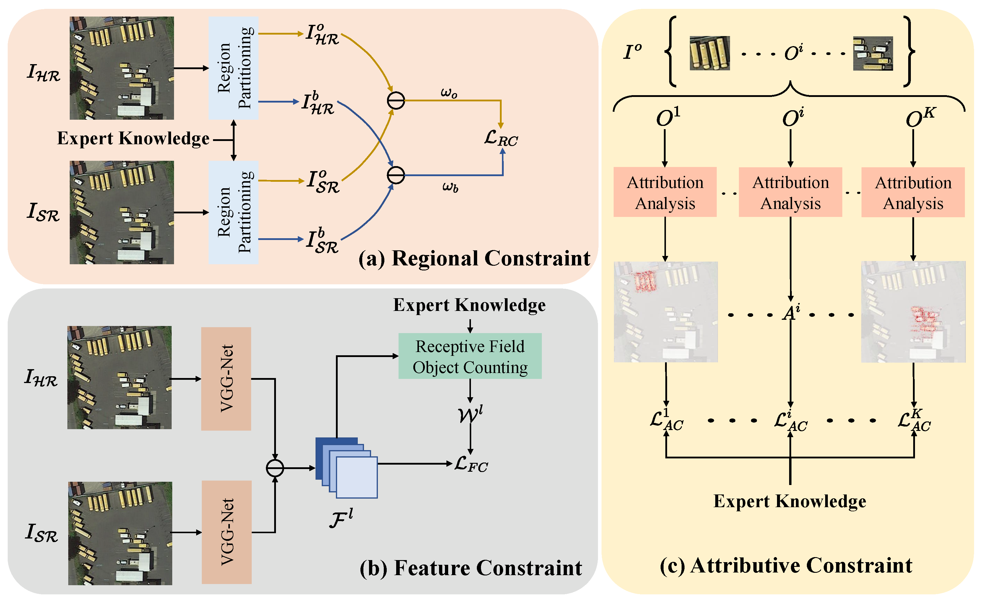
3.1. Regional Constraint

In the L1 loss function, $I^o$ and $I^b$ are treated equally, with the number of $I^b$ being larger than $I^o$. This makes it difficult for the SR model to learn the features of hard samples in $I^o$, resulting in unsatisfactory reconstruction results, as shown in Figure 1. To address this issue, we propose a regional constraint ${\mathcal{L}}_{RC}$, as shown in Figure 3a, which calculates the loss with adaptive weights for object region $I^o$ and background region $I^b$ based on expert-annotated prior knowledge from the high-level task.

Specifically, we divide an image I into two disjoint sets, $I^o$ and $I^b$, i.e., $I=I^o\cup I^b,I^o\cap I^b=⌀$. The object region $I^o$ is formed by taking the union of bounding boxes annotated by the experts, i.e., $I^o={\bigcup }_{i=0}^K{O}^i$. ${\mathcal{L}}_{RC}$ aims to enhance the SR model’s reconstruction performance on hard samples by selectively focusing on the foreground objects rather than the entire image. The regional constraint ${\mathcal{L}}_{RC}$ is defined as:

$$\begin{array}{ccc}& & {\mathcal{L}}_{RC}=w_o{∥I_{\mathcal{HR}}^o-I_{\mathcal{SR}}^o∥}_1+w_b{∥I_{\mathcal{HR}}^b-I_{\mathcal{SR}}^b∥}_1\hfill \\ & & \mathrm{s}.\mathrm{t}.w_o>0,w_b>0,w_o+w_b=1\hfill \end{array}$$

(5)

where $w_o$ and $w_b$ denote the learnable weights of the object region and the background region, respectively.

3.2. Feature Constraint

The perceptual loss ${\mathcal{L}}_{per}$ is typically used to extract the feature representation of an image using a pre-trained VGG network. The SR image is then constrained by minimizing the difference between the SR image and the HR image in the feature domain. However, perceptual loss only focuses on overall feature matching and neglects the local details. When an image contains many objects, ${\mathcal{L}}_{per}$ fails to pay sufficient attention to key features where the objects are located, resulting in SR images lacking details or appearing blurry.

To enhance the model’s ability to focus on key features during feature domain constraints, we measure the difficulty level of a feature ${\mathcal{F}}^l$ corresponding to the receptive field $M\left({\mathcal{F}}^l\right)$ extracted from the l-th layer of VGG by counting the number of object pixels ${\mathcal{W}}^l$ within it. This process can be described as follows:

$$\begin{array}{ccc}\hfill {\mathcal{F}}^l& =& {\varphi }_l\left(I_{\mathcal{HR}}\right)-{\varphi }_l\left(I_{\mathcal{SR}}\right)\hfill \end{array}$$

(6)

$$\begin{array}{ccc}\hfill P_{i,j}^l& =& \left\{\begin{array}{c}1,M\left({\mathcal{F}}_{i,j}^l\right)\in I^o\\ 0,M\left({\mathcal{F}}_{i,j}^l\right)\in I^b\end{array}\right.\hfill \end{array}$$

(7)

$$\begin{array}{ccc}\hfill {\mathcal{W}}^l& =& {∥P^l∥}_0\hfill \end{array}$$

(8)

where $M(·)$ represents a mapping relationship from the feature ${\mathcal{F}}^l$ to its receptive field on the original image I. Based on the difficulty level ${\mathcal{W}}^l$ of each feature’s corresponding receptive field, we propose the feature constraint ${\mathcal{L}}_{FC}$ shown in Figure 3b that incorporates expert knowledge. The expression is as

$$\begin{array}{c}\hfill {\mathcal{L}}_{FC}=\sum _{l=1}^n{\omega }_l({∥{\mathcal{F}}^l∥}_2^2\odot {\mathcal{W}}^l)\end{array}$$

(9)

where ⊙ denotes the element-wise product. ${\mathcal{L}}_{FC}$ weights each feature with ${\mathcal{W}}^l$, encouraging the model to pay more attention to hard samples that contain more objects, thereby achieving better reconstruction results.

3.3. Attributive Constraint

Due to the difficulty of fully annotating large-scale datasets, more explicit constraint methods are needed to guide the model learning, so that it can focus on the object regions even in the case of limited annotations. In previous work [52], it has been demonstrated that using bounding boxes for Attribution map (AM) supervision can guide high-level visual tasks. Specifically, the model’s results are more accurate when the model’s output relies more on the pixels inside the bounding box. However, the AM calculation and AM supervision progress are not suitable for the low-level task. Therefore, we have designed an attributive constraint based on AM supervision for the SR task as shown in Figure 3c, which can guide the SR model to pay more attention to the object region when reconstructing.

AM analysis [53,54,55,56] is an interpretability analysis method in DL used to explain the results of deep neural network models. For an input image $I\in {\mathbb{R}}^{h\times w}$ and a classification model $M:{\mathbb{R}}^{h\times w}\mapsto \mathbb{R}$, the model M can calculate the probability that input image I belongs to each category. The attribution analysis can output an AM for the importance of each pixel in the input image to the output of the model. Sundararajan et al. [55] proposed an Integrated Gradients (IG) method for attribution analysis and stated that the attribution analysis method should satisfy two basic axioms:

• Sensitivity: For any input image I and baseline image $I^{\prime }$, when any part of the image changes and causes a change in the model’s prediction result, the AM should also be able to express this change.
• Implementation Invariance: For two networks, even though their implementation methods are different, if their outputs are equal for all inputs, then the AM obtained by performing attribution analysis on these two networks should be the same.

Unlike high-level visual tasks that analyze attribution maps for a whole image, low-level visual tasks exhibit strong local correlations. Therefore, it is common to select a specific region for AM analysis. Local Attribution Maps (LAM) [57] is an AM analysis method for image SR tasks, which can identify which input pixels are important for the model’s output and their relative contribution levels. For LR image $I_{\mathcal{LR}}\in {\mathbb{R}}^{m/s\times n/s}$, SR image $I_{\mathcal{SR}}\in {\mathbb{R}}^{m\times n}$, and SR model $\mathcal{G}:{\mathbb{R}}^{m/s\times n/s}\mapsto {\mathbb{R}}^{m\times n}$ with upsample scale factor s, consider a patch $p\in {\mathbb{R}}^{q\times t}$ in the LR image and the range of patch is $[(p_{x1},p_{y1}),(p_{x2},p_{y2})]$. LAM designs the detector $D_p:{\mathbb{R}}^{q\times t}\mapsto \mathbb{R}$ to determine the edge feature.

$$\begin{array}{c}\hfill D_p\left(I\right)=\sum _{\begin{array}{c}i\in [p_{x1},p_{x2}]\\ j\in [p_{y1},p_{y2}]\end{array}}{\nabla }_{ij}I\end{array}$$

(10)

where ${\nabla }_{ij}I$ represents the gradient of image I at the pixel location $(i,j)$.

In the high-level attribution analysis method, the baseline image $I^{\prime }$ generally is a whole black image. However, for the SR task, the low-frequency component of the LR image is not important to the SR model performance and the high-frequency component is more important. Therefore, to decrease the high-frequency component in the input LR image I, LAM uses Gaussian blur to generate the baseline image $I^{\prime }$, which can be expressed as

$$\begin{array}{c}\hfill I^{\prime }=\omega \left(\sigma \right)\otimes I\end{array}$$

(11)

where $\omega \left(\sigma \right)$ is Gaussian blur kernel and the kernel size is $\sigma \times \sigma$. ⊗ denotes the convolution operation.

Let ${\gamma }_{\mathrm{pb}}=\left({\gamma }_{\mathrm{pb}}^1,\dots ,{\gamma }_{\mathrm{pb}}^n\right):[0,1]\to {\mathbb{R}}^n$ be a progressive blurring path function from the baseline image to the input image. It can be defined as follows:

$$\begin{array}{c}\hfill {\gamma }_{\mathrm{pb}}\left(\alpha \right)=\omega (\sigma -\alpha \sigma )\otimes I\end{array}$$

(12)

where ${\gamma }_{\mathrm{pb}}\left(0\right)=I^{\prime }$ and ${\gamma }_{\mathrm{pb}}\left(1\right)=I$.

The i-th dimension LAM ${LAM}_{F,D}{\left({\gamma }_{\mathrm{pb}}\right)}_i$ can be calculated by the IG method as follows:

$$\begin{array}{ccc}\hfill {LAM}_{F,D}{\left({\gamma }_{\mathrm{pb}}\right)}_i& =& {\int }_0^1{\displaystyle \frac{\partial D\left(F\left({\gamma }_{\mathrm{pb}}\left(\alpha \right)\right)\right)}{\partial {\gamma }_{\mathrm{pb}}{\left(\alpha \right)}_i}}\times {\displaystyle \frac{\partial {\gamma }_{\mathrm{pb}}{\left(\alpha \right)}_i}{\partial \alpha }}d\alpha \hfill \end{array}$$

(13)

$$\begin{array}{ccc}& \approx & \sum _{k=1}^m{\displaystyle \frac{\partial D\left(F\left({\gamma }_{\mathrm{pb}}\left(\frac{k}{m}\right)\right)\right)}{\partial {\gamma }_{\mathrm{pb}}{\left(\frac{k}{m}\right)}_i}}\times {\displaystyle \frac{\partial {\gamma }_{\mathrm{pb}}{\left(\frac{k}{m}\right)}_i}{\partial \left(\frac{k}{m}\right)}}\times {\displaystyle \frac{1}{m}}\hfill \end{array}$$

(14)

$$\begin{array}{ccc}& =& \sum _{k=1}^m{\displaystyle \frac{\left.\partial D\left(F\left({\gamma }_{\mathrm{pb}}\left(\frac{k}{m}\right)\right)\right)\right)}{\partial {\gamma }_{\mathrm{pb}}{\left(\frac{k}{m}\right)}_i}}\times {\left({\gamma }_{\mathrm{pb}}\left({\displaystyle \frac{k}{m}}\right)-{\gamma }_{\mathrm{pb}}\left({\displaystyle \frac{k+1}{m}}\right)\right)}_i\hfill \end{array}$$

(15)

where Equations (14) and (15) are the approximations of Equation (13) that can make the calculation faster. m is the step number in the approximation of the integral. The entire LAM ${LAM}_{F,D}\left({\gamma }_{\mathrm{pb}}\right)$ can be calculated as

$$\begin{array}{ccc}\hfill {LAM}_{F,D}\left({\gamma }_{\mathrm{pb}}\right)& =& \sum _i{LAM}_{F,D}{\left({\gamma }_{\mathrm{pb}}\right)}_i\hfill \end{array}$$

(16)

$$\begin{array}{ccc}& =& D\left(F\left(I\right)\right)-D\left(F\left(I^{\prime }\right)\right)\hfill \end{array}$$

(17)

To determine which pixels and their relative contribution levels are used by the SR model to reconstruct each object’s region $O^i$, we perform AM analysis on $O^i$ separately, resulting in the corresponding AM $A^i$. This process can be described as follows:

$$\begin{array}{cc}\hfill A^i& ={LAM}_{\mathcal{G},D,O^i}\left({\gamma }_{\mathrm{pb}}\right),i=1,2,\dots ,K\end{array}$$

(18)

where ${LAM}_{\mathcal{G},D,O^i}\left({\gamma }_{\mathrm{pb}}\right)$ denotes the calculation process of the AM on the patch $O^i$ of image I and the model is generator network $\mathcal{G}$.

Furthermore, we define the AM in the object region $A^{i+}=A^i\cap O^i$, which represents a collection of pixels used by the SR model to reconstruct the region where the object is located. Let $v\left(A\right)={\sum }_{m=1}^h{\sum }_{n=1}^w{A}_{m,n}:{\mathbb{R}}^{h\times w}\mapsto \mathbb{R}$ be a function that sums up the relative contribution level in AM A. To achieve better SR results, we should increase the constraint for the model to utilize pixels located within the bounding box as much as possible. This is equivalent to maximizing the ratio of $v\left(A^{i+}\right)/v\left(A^i\right)$. Therefore, the attributive constraint ${\mathcal{L}}_{AC}$ is defined as follows:

$$\begin{array}{ccc}\hfill {\mathcal{L}}_{AC}& =& {\displaystyle \frac{1}{K}}\sum _{i=1}^K\left({\mathcal{L}}_{AC}^i\right)\hfill \end{array}$$

(19)

$$\begin{array}{ccc}& =& {\displaystyle \frac{1}{K}}\sum _{i=1}^K(1-{\displaystyle \frac{v\left(A^{i+}\right)}{v\left(A^i\right)}})\hfill \end{array}$$

(20)

where ${\mathcal{L}}_{AC}^i$ represents the each attributive constraint to i-th object’s region.

3.4. Proposed Learning Strategy

Based on the analysis in the previous sections, we have derived three different SR loss functions ${\mathcal{L}}_{RC}$, ${\mathcal{L}}_{FC}$, and ${\mathcal{L}}_{AC}$ that incorporate expert knowledge from different perspectives. To obtain a more versatile learning strategy, we have designed two distinct loss functions, ${\mathcal{L}}_{PSNR}$ and ${\mathcal{L}}_{GAN}$, specifically targeting PSNR-SR and GAN-SR methods, respectively. The loss functions are defined as

$$\begin{array}{cc}& {\mathcal{L}}_{PSNR}={\mathcal{L}}_{RC}+{10}^{-4}{\mathcal{L}}_{AC}\end{array}$$

(21)

$$\begin{array}{cc}& {\mathcal{L}}_{GAN}=\xi {\mathcal{L}}_{RC}+\mu {\mathcal{L}}_{FC}+\delta {\mathcal{L}}_{adv}+{10}^{-4}\xi {\mathcal{L}}_{AC}\end{array}$$

(22)

where $\xi$, $\mu$, and $\delta$ denote the different weights of each component to ensure that no individual loss dominates and impedes convergence. In this work, we set it to $1\times {10}^{-2},1$, and $5\times {10}^{-3}$ follow previous literature [20]. ${\mathcal{L}}_{GAN}$ incorporates ${\mathcal{L}}_{FC}$ and ${\mathcal{L}}_{adv}$ based on ${\mathcal{L}}_{PSNR}$ to enhance the visual quality and detail fidelity.

Since the model cannot obtain accurate attribution maps in the initial stages of training, using ${\mathcal{L}}_{AC}$ in the early training phase can cause network oscillation and make convergence difficult. Therefore, we introduce ${\mathcal{L}}_{AC}$ after 10,000 iterations to guide the model to utilize more effective pixels for SR reconstruction. Meanwhile, we noticed that the computation of LAM takes a longer time. To avoid significantly increasing the training time, we perform ${\mathcal{L}}_{AC}$ calculation every 100 iterations. The overview of the proposed learning strategy is presented in Algorithm 1.

Algorithm 1 EKS-SR Learning Strategy

Input: A dataset of image pairs with expert knowledge $\left\{(I_{\mathcal{HR}},I_{\mathcal{LR}},O^i)\right\}$, Initial model parameters $\Theta$, Number of iterations $N_{iter}$, Start iterations of attribute constraint begins $N_{AC}$, Attributive constraint frequency f.

Output: Trained model parameters $\widehat{\Theta }$

1: for $i=1$ to $N_{iter}$ do 2:     $I_{\mathcal{SR}}\leftarrow \Theta \left(I_{\mathcal{LR}}\right)$ 3:     $l_{RC}\leftarrow {\mathcal{L}}_{RC}(I_{\mathcal{HR}},I_{\mathcal{SR}})$ 4:     if $i>N_{AC}$ and $\mathrm{mod}(i,f)$ = 0 then 5:         $A^i\leftarrow f_{att}\left(O^i\right)$ 6:         $l_{AC}\leftarrow {\mathcal{L}}_{AC}(I_{\mathcal{HR}},I_{\mathcal{SR}},A^i)$ 7:     else 8:         $l_{AC}\leftarrow 0$ 9:     end if 10:     if $\Theta$ is a PSNR-SR model then 11:         $l_{PSNR}\leftarrow l_{RC}+{10}^{-4}{l}_{AC}$ 12:     else $\Theta$ is a GAN-SR model 13:         $l_{adv}\leftarrow {\mathcal{L}}_{adv}\left(I_{\mathcal{SR}}\right)$ 14:         $l_{FC}\leftarrow {\mathcal{L}}_{FC}(I_{\mathcal{HR}},I_{\mathcal{SR}})$ 15:         $l_{GAN}\leftarrow \xi l_{RC}+\mu l_{FC}+\delta l_{adv}+{10}^{-4}\xi l_{AC}$ 16:     end if 17:     Update $\Theta$ with the Adam Optimizer 18: end for 19: return $\widehat{\Theta }=\Theta$

4. Experiments

4.1. Datasets and Evaluation Metrics

4.1.1. Datasets Description

In this work, we select Instance Segmentation in Aerial Images Dataset (iSAID) [58] and Cars Overhead With Context (COWC) [59] public datasets for evaluation.

(1)

iSAID: The iSAID dataset consists of 2806 images with different sizes and 655,451 annotated instances. Due to the large size of the original images in the iSAID dataset, we have divided them into $800\times 800$ image patches for training and testing. We have created the SR dataset using bicubic and Gaussian blur to get the LR image with $200\times 200$ sizes. The original training set is used as the training set for the SR task. Additionally, the validation set of iSAID is used as the test set for the SR task. The training set contains a total of 27,286 images and the test set contains a total of 9446 images.

(2)

COWC: The COWC is a large dataset of annotated cars from overhead, which consists of images from Selwyn in New Zealand, Potsdam and Vaihingen in Germany, Columbus and Utah in the United States, and Toronto in Canada. We crop the image to $256\times 256$ and randomly select 80% images in Potsdam for training, 10% images in Potsdam for validating, and others for testing. The LR images of the COWC dataset have a size of $64\times 64$ and $32\times 32$, corresponding to $\times 4$ and $\times 8$ upscale factor SR tasks, respectively.

4.1.2. Evaluation Metrics for SR

We select PSNR, Structural Similarity Index (SSIM), and Learned Perceptual Image Patch Similarity (LPIPS) [60] as evaluation metrics for the SR task.

(1)

PSNR: PSNR is the most widely used objective quality assessment metric in SR tasks. Given HR image $I_{\mathcal{HR}}$ and LR image $I_{\mathcal{SR}}$, PSNR is defined as

$$\mathrm{PSNR}(I_{\mathcal{HR}},I_{\mathcal{SR}})=10·{log}_{10}\left({\displaystyle \frac{{\mathrm{MAX}}_I^2}{\mathrm{MSE}(I_{\mathcal{HR}},I_{\mathcal{SR}})}}\right)$$

(23)

where ${\mathrm{MAX}}_I$ represents the maximum pixel value (255 for 8-bit images) and $\mathrm{MSE}(I_{\mathcal{HR}},I_{\mathcal{SR}})$ represents the mean squared error (MSE) between $I_{\mathcal{HR}}$ and $I_{\mathcal{SR}}$, which can be calculated as

$$\mathrm{MSE}(I_{\mathcal{HR}},I_{\mathcal{SR}})={\displaystyle \frac{1}{mn}}\sum _{i=0}^{m-1}\sum _{j=0}^{n-1}{[I_{\mathcal{HR}}(i,j)-I_{\mathcal{SR}}(i,j)]}^2$$

(24)

where m and n represent the height and width of the SR image $I_{\mathcal{SR}}$. A larger PSNR value indicates greater similarity between the two images.

(2)

SSIM: SSIM is an index that quantifies the structural similarity between two images. Unlike PSNR, SSIM is designed to mimic the human visual system’s perception of structural similarity. SSIM quantifies the image’s attributes of brightness, contrast, and structure, using the mean to estimate brightness, variance to estimate contrast, and covariance to estimate structural similarity. SSIM is defined as

$$\mathrm{SSIM}(I_{\mathcal{HR}},I_{\mathcal{SR}})={\displaystyle \frac{(2{\mu }_x{\mu }_y+C_1)(2{\sigma }_{xy}+C_2)}{({\mu }_x^2+{\mu }_y^2+C_1)({\sigma }_x^2+{\sigma }_y^2+C_2)}}$$

(25)

where ${\mu }_x$ and ${\mu }_y$ denote the mean values of $I_{\mathcal{HR}}$ and $I_{\mathcal{SR}}$, respectively. ${\sigma }_x^2$ and ${\sigma }_y^2$ denote the variance of $I_{\mathcal{HR}}$ and $I_{\mathcal{SR}}$, respectively. ${\sigma }_{xy}$ denotes the covariance of $I_{\mathcal{HR}}$ and $I_{\mathcal{SR}}$. $C_1$ and $C_2$ are two constants used to maintain the stability of the denominator. The SSIM value ranges from 0 to 1, with a higher value indicating greater similarity between the two images.

(3)

LPIPS: To better simulate human visual perception, Zhang et al. [60] proposed LPIPS, which measures the difference between two images in the feature domain by a pre-trained VGG [51] feature extract network $\phi$. Compared to PSNR and SSIM, LPIPS evaluates the similarity between two images in a way that is more consistent with human visual habits. LPIPS is defined as

$$\mathrm{LPIPS}(I_{\mathcal{HR}},I_{\mathcal{SR}})=\sum _{l=1}^L{\displaystyle \frac{1}{H_l{W}_l}}\sum _{h,w}{∥\eta \odot \left({\phi }_{h,w}^l\left(I_{\mathcal{HR}}\right)-{\phi }_{h,w}^l\left(I_{\mathcal{SR}}\right)\right)∥}_2^2$$

(26)

where ${\phi }_{h,w}^l$ and $\eta$ represents the l-th layer of $\phi$ and its weights. $H_l$ and $W_l$ is the height and width of the SR image $I_{\mathcal{SR}}$. A smaller LPIPS value indicates greater similarity between the two images.

4.1.3. Evaluation Metrics for Object Detection and Instance Segmentation

We use COCO evaluation metrics for object detection and instance segmentation tasks. This includes $A{P}^b$ and $A{P}^m$ for bounding boxes and masks, which measures the average precision (AP) values for ten intersections over union (IoU) thresholds ranging from 0.5 to 0.95. Specifically, $A{P}_{50}^b$, $A{P}_{50}^m$, $A{P}_{75}^b$, and $A{P}_{75}^m$ represent the AP values for detection and segmentation at IoU thresholds of 0.5 and 0.75, respectively. The object detection task use $A{P}^b$, $A{P}_{50}^b$, and $A{P}_{75}^b$ as evaluation metrics. The instance segmentation task uses all six metrics.

4.2. Implementation Details

To validate the effectiveness of our proposed EKS-SR, we select three classical SR works SRGAN [20], SRFormer [46], and SwinIR [16], which have been widely used in SR fields and represent GAN-SR and PSNR-SR, respectively. For the training of the SR model, we train it on patches of size 256 × 256. For the SR models SRGAN and SwinIR, the batch sizes are set to 32 and 16, respectively. The initial learning rate is $2\times {10}^{-4}$ and decreases to half in 50,000, 100,000, and 200,000 iterations. We use the Adam optimizer [61] by setting ${\beta }_1=0.9$, ${\beta }_2=0.99$, and $ϵ={10}^{-8}$ to optimize the SR models. All SR models are trained for 300,000 iterations.

Furthermore, we use the Faster region-based Convolutional Neural Network (Faster R-CNN) [62] model as the object detection network to evaluate the SR images obtained from different SR models. For the instance segmentation task evaluation, we select the Mask region-based Convolutional Neural Network (Mask R-CNN) [29] model with a ResNet101 [30] as the backbone. The Faster R-CNN and Mask R-CNN are trained on the HR images in the original dataset. For Faster R-CNN, we use the Adam optimizer [61] by setting ${\beta }_1=0.9$, ${\beta }_2=0.99$, and $ϵ={10}^{-8}$ for training. For Mask R-CNN, we use the stochastic gradient descent with momentum of 0.9 and weight decay of 0.0001 as the optimizer to train the entire network. The experiments are implemented under NVIDIA RTX 3090 graphics processing unit (GPU) and Ubuntu 18.04.

4.3. Results Achieved Using the Learning Strategy EKS-SR on Different SR Models

To demonstrate the effectiveness of our proposed learning strategy, EKS-SR, we conducted training on three representative works in the existing two major categories of SR methods: SRGAN [20], SRFormer [46], and SwinIR [16]. We then utilized models trained under different learning strategies to obtain SR images. Specifically, we trained the SR model using three different approaches: the original learning strategy, locally discriminative learning (LDL) [63], and our proposed EKS-SR, respectively. Additionally, we input the LR images into the SR model to reconstruct the SR images. Finally, we input the SR images into the same pre-train Faster R-CNN or Mask R-CNN network to obtain object detection and instance segmentation results.

4.3.1. Quantitative Results on COWC

As shown in

Table 1. Results of comparison with different learning strategies on the $\times 4$ COWC dataset. The best result of each metric is in bold font.

Model	Learning Strategy	PSNR ↑	SSIM ↑	LPIPS ↓	${\mathit{AP}}^{\mathit{b}}$↑	${\mathit{AP}}_{50}^{\mathit{b}}$↑	${\mathit{AP}}_{75}^{\mathit{b}}$↑
HR	-	-	-	-	93.7	97.7	97.6
SRGAN	Original	26.526	0.6283	0.3687	41.5	62.3	47.8
	LDL	27.432	0.6518	0.3488	48.1	68.6	57.3
	EKS-SR	27.083	0.6359	0.3471	51.3	73.0	61.7
SRFormer	Original	31.580	0.8033	0.3488	70.5	84.7	82.1
	LDL	27.689	0.6697	0.3412	48.8	71.4	58.3
	EKS-SR	32.348	0.8263	0.3233	77.5	88.7	87.7
SwinIR	Original	33.205	0.8500	0.2922	80.5	90.8	89.7
	LDL 1	28.704	0.6847	0.4035	37.0	50.8	44.4
	LDL 2	27.313	0.6219	0.2583	57.4	79.4	70.0
	EKS-SR	33.220	0.8505	0.2912	80.8	90.9	89.8

¹ These results are obtained using the weights trained on the DF2K dataset provided in link https://github.com/csjliang/LDL, accessed on 31 July 2024. ² These results are obtained using the weights trained on the COWC dataset.

, the SRGAN and SwinIR trained by the EKS-SR can achieve performance improvement on three SR evaluation metrics and three object detection metrics. Specifically, EKS-SR demonstrates a significant improvement over SRGAN in the object detection task, with enhancements of 9.8, 10.7, and 13.9 across three evaluation metrics, respectively. Moreover, the SR model also achieved better visual performance, with increases of 0.557, 0.0760, and 0.0216 in PSNR, SSIM, and LPIPS, respectively. Although SwinIR has a larger number of parameters and higher computational complexity, it already achieves good visual effects and object detection results using the original SR learning strategy. However, EKS-SR, guided by expert knowledge, can more deeply explore the key information in the regions where objects are located within the image, making the SR model learn more effectively and enhancing its image reconstruction capabilities. Consequently, the six metrics obtained by the SwinIR model exhibit improvements.

We compare the three models based on different learning strategies, including original, LDL, and our proposed EKS-SR. For SRGAN, a representative work of GAN-SR, the model obtained using the EKS-SR learning strategy gave the best performance in the object detection task. Although LDL shows a larger increase in PSNR and SSIM metrics than EKS-SR, the gain is limited in practical applications. For the SRFormer model, the use of the EKS-SR learning strategy gives the best results in both SR metrics and object detection metrics, while the use of the LDL method instead results in a decrease in accuracy in the object detection task. For the SwinIR model, we compare the results of the model pre-trained on the DF2K [64,65] dataset and our implementation model trained on the COWC dataset. It can be observed that although LDL can improve the LPIPS metrics, the accuracy drop on the object detection task is severe. This indicates that EKS-SR has better utility than LDL.

The experimental results reveal that LDL can improve the visual quality of the image by removing artifacts, which makes some progress in SR metrics, but brings about a performance degradation in real-world RS applications. In contrast, with the regional constraint, feature constraint, and attributive constraint, EKS-SR can make the SR model pay more attention to complex object regions in RS images during the training process, which can enhance the visual quality of SR images and improve the performance of practical tasks.

4.3.2. Quantitative Results on iSAID

Table 2. Results of comparison with different learning strategies on the $\times 4$ iSAID dataset. The best result of each metric is in bold font.

Model	Learning Strategy	PSNR ↑	SSIM ↑	LPIPS ↓	${\mathit{AP}}^{\mathit{b}}$↑	${\mathit{AP}}_{50}^{\mathit{b}}$↑	${\mathit{AP}}_{75}^{\mathit{b}}$↑	${\mathit{AP}}^{\mathit{m}}$↑	${\mathit{AP}}_{50}^{\mathit{m}}$↑	${\mathit{AP}}_{75}^{\mathit{m}}$↑
HR	-	-	-	-	44.2	63.1	46.7	36.5	59.3	39.4
SRGAN	Original	35.299	0.8516	0.2219	36.4	55.9	39.8	29.2	49.2	30.6
	EKS-SR	36.352	0.8680	0.2041	37.2	56.7	41.0	29.8	50.4	31.3
	Improvement	1.053	0.0164	0.0178	0.8	0.8	1.2	0.6	1.2	0.7
SwinIR	Original	38.533	0.9011	0.2182	37.8	57.0	41.7	30.7	50.9	32.9
	EKS-SR	38.550	0.9015	0.2170	37.9	57.2	41.8	30.8	51.0	32.9
	Improvement	0.017	0.0004	0.0012	0.1	0.2	0.1	0.1	0.1	0.0

presents the results of SRGAN and SwinIR using different learning strategies for upscale $\times 4$. For the PSNR-SR method SwinIR, the original learning strategy has already yielded favorable results with a PSNR of 38.533 dB. However, models trained using EKS-SR still can achieve a gain of 0.017 dB. It is important to note that PSNR is a logarithmic scale metric, where even small numerical changes correspond to significant perceptual variations. Additionally, in terms of human perception, EKS-SR can enhance the LPIPS metric by $4\%$ compared to SwinIR. For the GAN-SR method SRGAN, the original learning strategy exhibited notable shortcomings. Thanks to the utilization of expert knowledge supervision in EKS-SR, SRGAN can achieve an improvement of 1.053 dB in PSNR, along with enhancements of 0.0164 in SSIM and 0.0178 in LPIPS.

Meanwhile, it can be observed that the models trained using the EKS-SR learning strategy show improvements in all six metrics, whether in the PSNR-SR model or the GAN-SR model. Additionally, for the smaller-scale SRGAN network, employing the EKS-SR learning strategy significantly narrows the performance gap between it and the larger SwinIR model in practical tasks. With advanced learning strategies, satisfactory performance can be achieved even with smaller models, making significant contributions to the practical application of DL models in the resource-limited RS device.

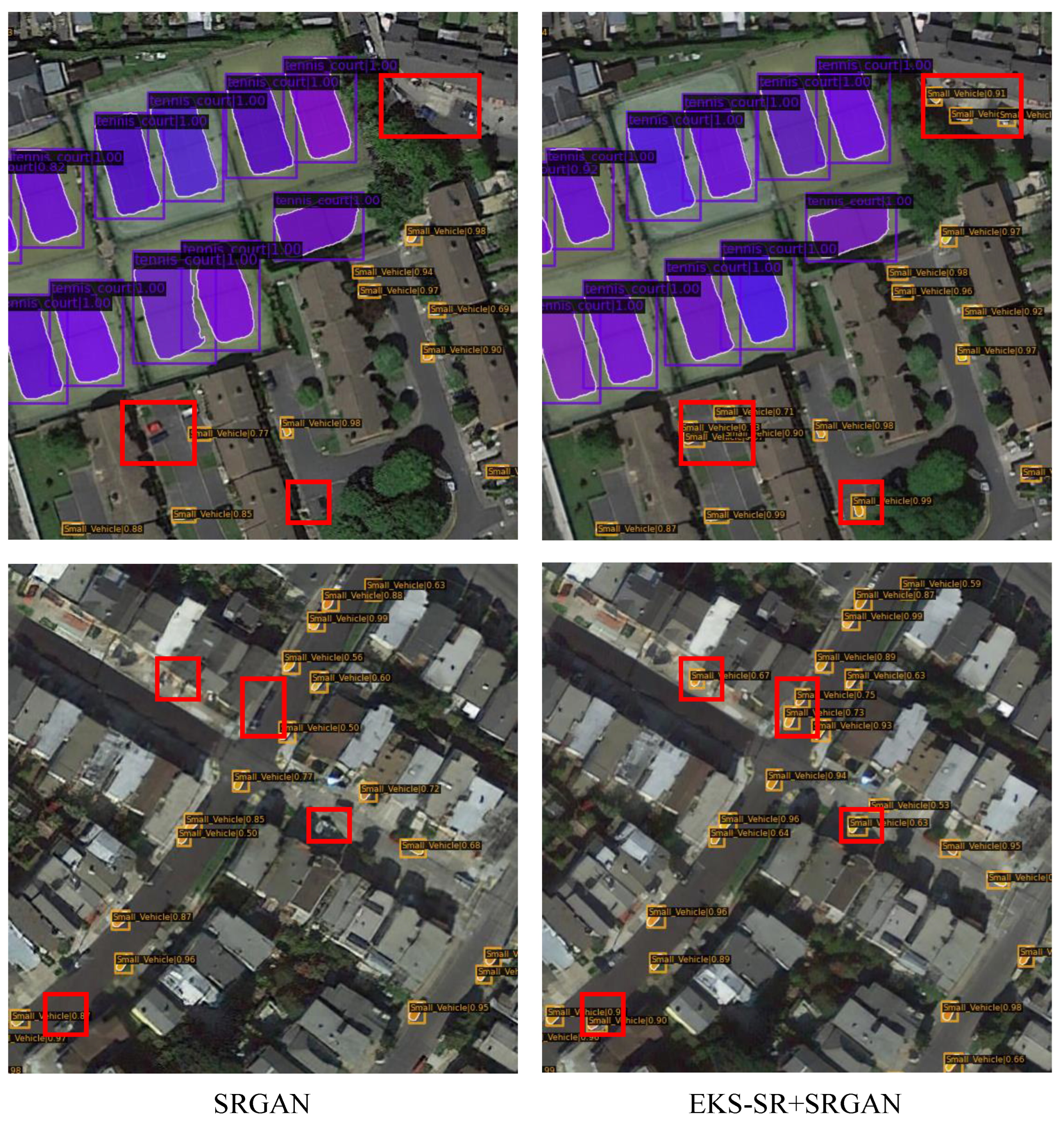
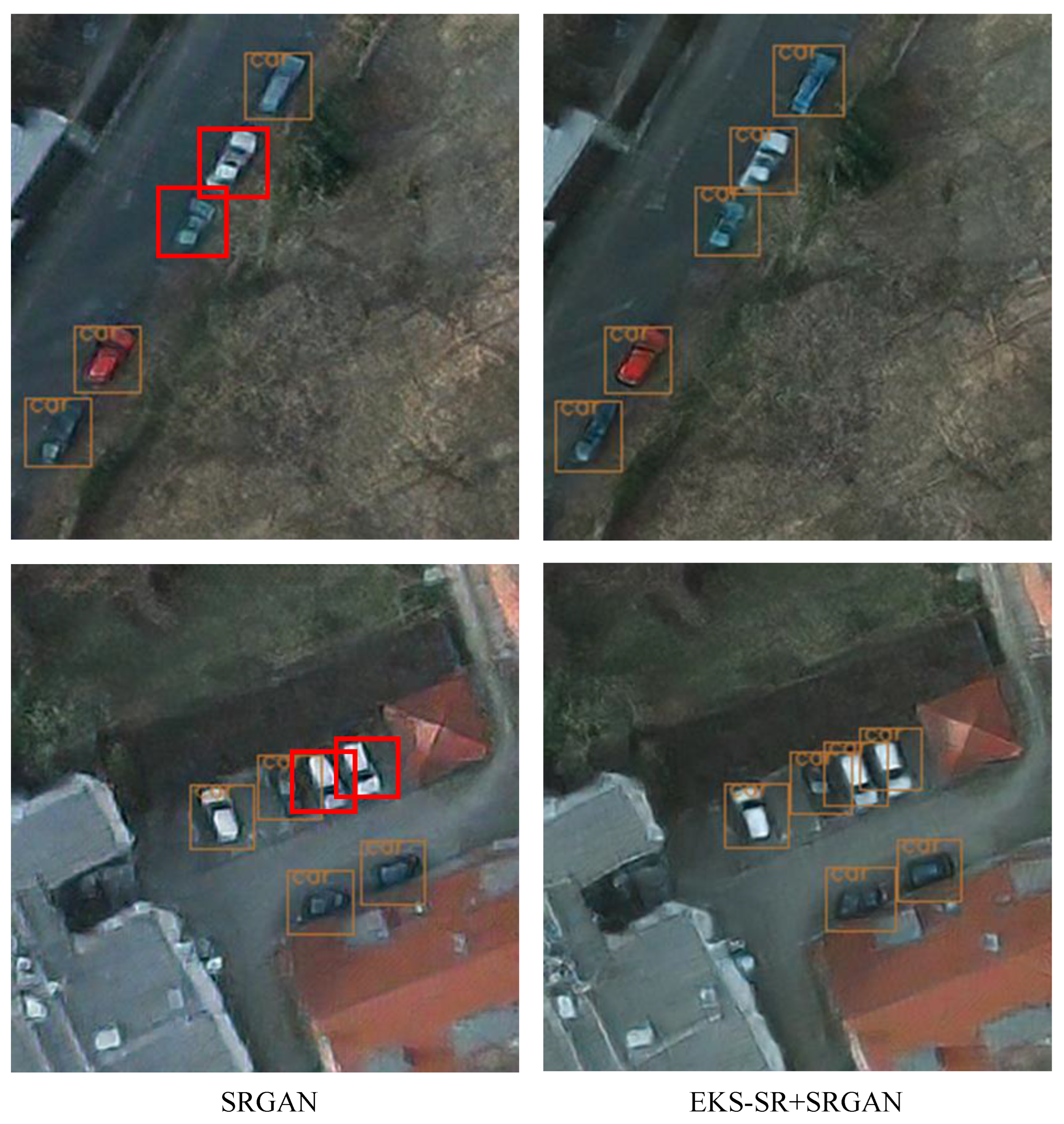
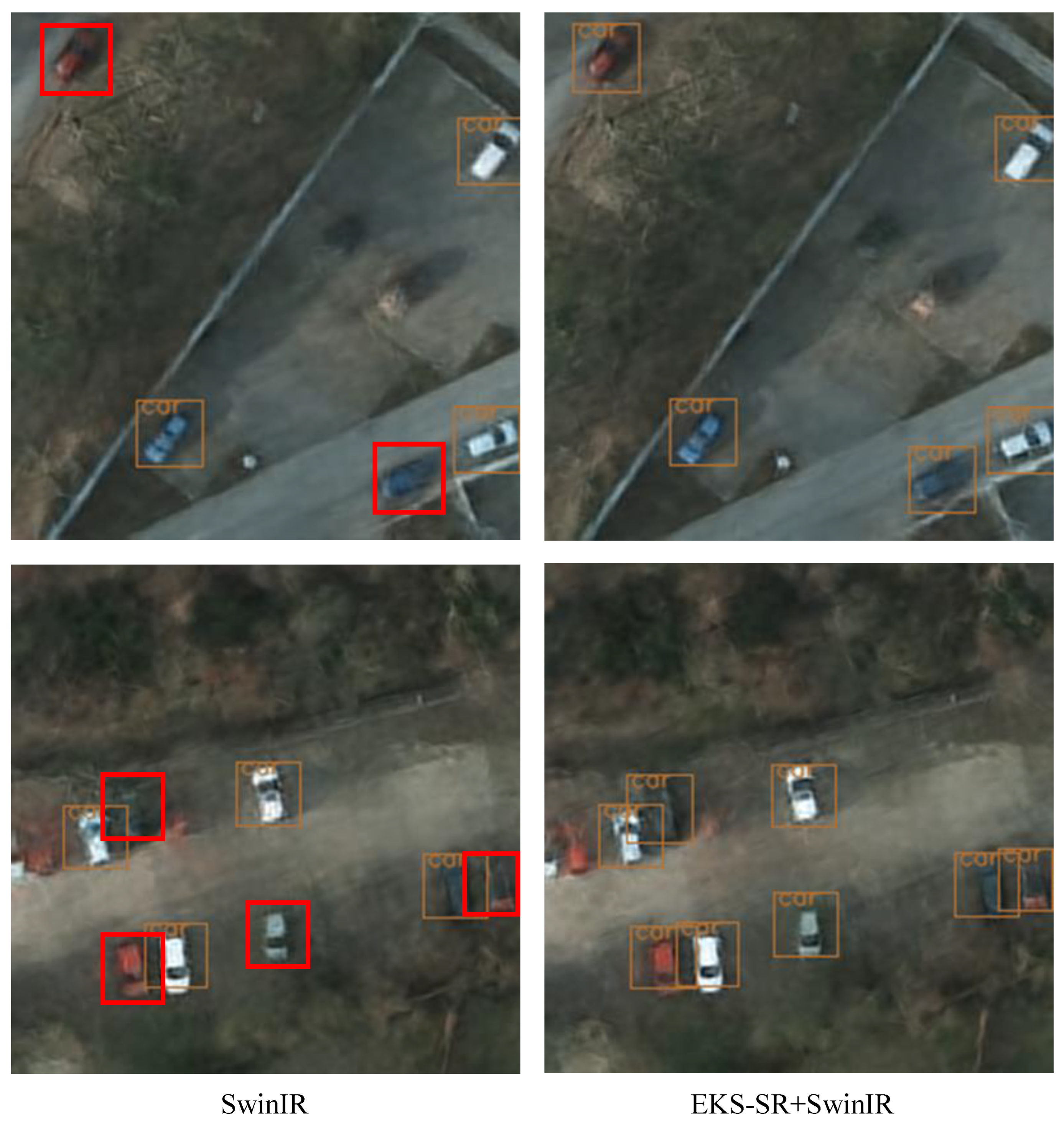
4.3.3. Qualitative Comparison

To intuitively compare the performance of EKS-SR in practical applications, we have visualized the instance segmentation results on the iSAID dataset, as shown in Figure 4, and the object detection results on the COWC dataset are shown in Figure 5 and Figure 6. It can be seen that the SR images reconstructed by the SR model using the original learning strategy fail to be detected by the instance segmentation model in many areas, especially for small objects. This is because small objects tend to lose their original structure and become more difficult to reconstruct after degradation. In contrast, the SR model trained with EKS-SR demonstrates a significant improvement in this problem, which indicates that EKS-SR has strong practical application value and can effectively mitigate the issues associated with severe degradation of RS images. Consequently, EKS-SR contributes to improved performance in various machine vision applications.

4.4. Performance under Different Upscale Factors

To validate the applicability of the proposed EKS-SR learning strategy in SR tasks with different upscale factors, we conducted comparative experiments using the SwinIR model on the COWC dataset with $\times 4$ and $\times 8$ upscale factors. Specifically, we trained the SR network with both the original and EKS-SR learning strategies at $\times 4$ and $\times 8$ upscale factors, respectively.

As shown in

Table 3. Results of comparison with different learning strategies on the $\times 4$ and $\times 8$ COWC dataset. The best result of each metric is in bold font.

Upscale	Learning Strategy	PSNR ↑	SSIM ↑	LPIPS ↓	${\mathit{AP}}^{\mathit{b}}$↑	${\mathit{AP}}_{50}^{\mathit{b}}$↑	${\mathit{AP}}_{75}^{\mathit{b}}$↑
HR	-	-	-	-	93.7	97.7	97.6
$\times 4$	Original	33.205	0.8500	0.2922	80.5	90.8	89.7
	EKS-SR	33.220	0.8505	0.2912	80.8	90.9	89.8
	Improvement	0.015	0.0005	0.0010	0.3	0.1	0.1
$\times 8$	Original	29.469	0.7655	0.3987	50.6	63.8	60.3
	EKS-SR	29.567	0.7690	0.3953	52.9	66.5	62.5
	Improvement	0.098	0.0035	0.0034	2.3	2.7	2.2

, the results obtained by the SR model for images downsampled by a factor of eight are significantly inferior to those for images downsampled by a factor of four. This is due to the greater information loss caused by $\times 8$ downsampling, which substantially increases the reconstruction difficulty. Additionally, the accuracy of SR images in the object detection task drops significantly, with $A{P}^b$ decreasing from 80.5 to 50.6. However, training with the EKS-SR learning strategy yields greater gains in both visual quality and practical tasks. This indicates that EKS-SR can still assist the SR model in identifying more complex object regions within highly degraded images, thereby achieving better SR reconstruction performance. Figure 6 and Figure 7 show the object detection results on the $\times 4$ and $\times 8$ COWC datasets.

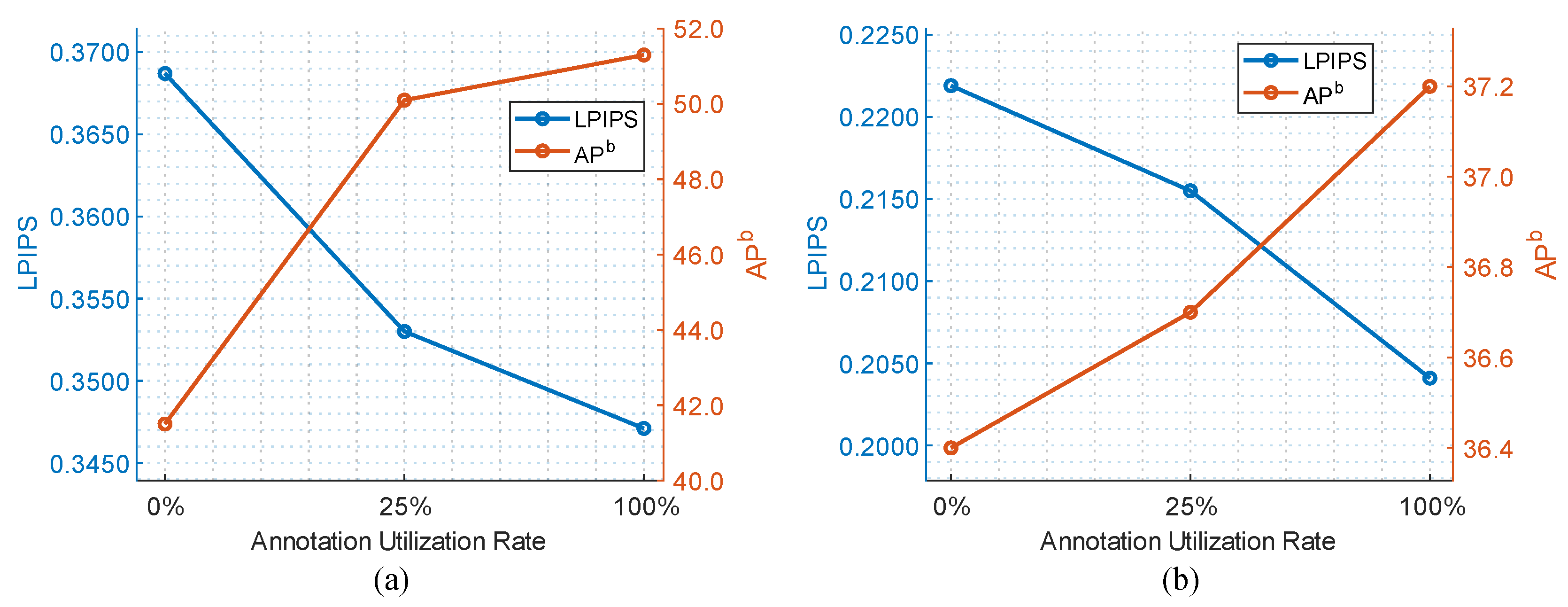
4.5. Performance under Limited Annotation

Annotating large datasets comprehensively is an extremely challenging task. To validate the performance of EKS-SR with limited annotations, we constrained the model using only $25\%$ of the annotations.

As shown in

Table 4. Comparison results of different label utilization rates on SRGAN from $\times 4$ iSAID dataset.

Label Utilization Rate	PSNR ↑	SSIM ↑	LPIPS ↓	${\mathit{AP}}^{\mathit{b}}$↑	${\mathit{AP}}_{50}^{\mathit{b}}$↑	${\mathit{AP}}_{75}^{\mathit{b}}$↑	${\mathit{AP}}^{\mathit{m}}$↑	${\mathit{AP}}_{50}^{\mathit{m}}$↑	${\mathit{AP}}_{75}^{\mathit{m}}$↑
100%	36.352	0.8680	0.2041	37.2	56.7	41.0	29.8	50.4	31.3
25%	35.960	0.8520	0.2155	36.7	56.3	40.4	29.4	49.9	30.6
0%	35.299	0.8516	0.2219	36.4	55.9	39.8	29.2	49.2	30.6

and

Table 5. Comparison results of different label utilization rates on SRGAN from $\times 4$ COWC dataset.

Label Utilization Rate	PSNR ↑	SSIM ↑	LPIPS ↓	${\mathit{AP}}^{\mathit{b}}$↑	${\mathit{AP}}_{50}^{\mathit{b}}$↑	${\mathit{AP}}_{75}^{\mathit{b}}$↑
100%	27.083	0.6359	0.3471	51.3	73.0	61.7
25%	26.819	0.6261	0.3530	50.1	70.7	60.7
0%	26.526	0.6283	0.3687	41.5	62.3	47.8

, the results indicate that even using a small number of bounding box annotations can effectively guide the model to focus on the object regions in the image. Figure 8 intuitively compares LPIPS and $A{P}^b$ across various annotation utilization rates. Despite the model using only $25\%$ of the annotations, the SRGAN model trained by the EKS-SR also gets 0.661 dB on the iSAID dataset and 0.293 dB on the COWC dataset. Meanwhile, the LPIPS metric showed enhancements of 0.0064 and 0.0157, respectively. Furthermore, for the instance segmentation task, the five metrics have been improved by the EKS-SR under limited annotation. For the object detection task, the increases achieved in three evaluation metrics are 8.6, 8.4, and 12.9, respectively. It should be noted that the gains obtained by using only $25\%$ annotations in machine vision applications are already close to the gains obtained by using $100\%$ annotations, which are 9.8, 10.7, and 13.9, respectively. The proposed learning strategy EKS-SR not only enhances the detection performance of objects but also improves the effectiveness of fine-grained semantic segmentation tasks, further confirming the practicality.

4.6. Ablation Studies

To validate the effectiveness of all three constraints in EKS-SR, we designed various learning strategies for conducting ablation experiments. Specifically, we replaced ${\mathcal{L}}_1$ with ${\mathcal{L}}_{RC}$ and ${\mathcal{L}}_{per}$ with ${\mathcal{L}}_{FC}$ in the original SRGAN, and the results are shown in

Table 6. Ablation results of comparison with different learning strategies on the iSAID dataset. The best result of each metric is in bold font.

Model	Learning Strategy	PSNR ↑	SSIM ↑	LPIPS ↓	${\mathit{AP}}^{\mathit{b}}$↑	${\mathit{AP}}_{50}^{\mathit{b}}$↑	${\mathit{AP}}_{75}^{\mathit{b}}$↑	${\mathit{AP}}^{\mathit{m}}$↑	${\mathit{AP}}_{50}^{\mathit{m}}$↑	${\mathit{AP}}_{75}^{\mathit{m}}$↑
HR	-	-	-	-	44.2	63.1	46.7	36.5	59.3	39.4
SRGAN	${\mathcal{L}}_1$ + ${\mathcal{L}}_{per}$ + ${\mathcal{L}}_{adv}$	35.299	0.8516	0.2219	36.4	55.9	39.8	29.2	49.2	30.6
	${\mathcal{L}}_{RC}$ + ${\mathcal{L}}_{per}$ + ${\mathcal{L}}_{adv}$	35.822	0.8516	0.2213	36.4	55.8	39.9	29.2	49.1	30.4
	${\mathcal{L}}_{RC}$ + ${\mathcal{L}}_{FC}$ + ${\mathcal{L}}_{adv}$	36.001	0.8511	0.2094	36.9	56.5	40.5	29.6	50.2	30.8
	${\mathcal{L}}_{RC}$ + ${\mathcal{L}}_{FC}$ + ${\mathcal{L}}_{AC}$ + ${\mathcal{L}}_{adv}$	36.352	0.8680	0.2041	37.2	56.7	41.0	29.8	50.4	31.3
SwinIR	${\mathcal{L}}_1$	38.533	0.9011	0.2182	37.8	57.0	41.7	30.7	50.9	32.9
	${\mathcal{L}}_{RC}$	38.541	0.9012	0.2178	37.9	57.1	41.9	30.7	51.0	32.7
	${\mathcal{L}}_{RC}$ + ${\mathcal{L}}_{AC}$	38.550	0.9015	0.2170	37.9	57.2	41.8	30.8	51.0	32.9

. It can be seen that when ${\mathcal{L}}_{RC}$ is used alone, there is an improvement of 0.523 dB in PSNR. When ${\mathcal{L}}_{RC}$ and ${\mathcal{L}}_{FC}$ are used together, not only is a gain of 0.702 dB in PSNR achieved, but also gains of 0.5 and 0.4 in $A{P}^b$ and $A{P}^m$, respectively. This demonstrates the effectiveness of ${\mathcal{L}}_{RC}$ and ${\mathcal{L}}_{FC}$. Additionally, experiments on the SwinIR model verified the effectiveness of ${\mathcal{L}}_{RC}$ and ${\mathcal{L}}_{AC}$. The ablation experiments suggest that these proposed constraints play a vital role in achieving SR reconstruction and high-level task performances.

5. Discussion

This work proposes a new SR learning strategy based on expert knowledge supervision, aiming to address the shortcomings of existing SR methods in practical applications. EKS-SR successfully integrates expert knowledge from high-level vision tasks into the SR reconstruction process, significantly improving the model’s ability to reconstruct object regions in low-resolution images, especially for small objects. Experimental results show that EKS-SR not only improves the visual quality but more importantly achieves significant performance improvements in downstream tasks such as object detection and instance segmentation. This confirms the effectiveness of our approach in bridging the gap between low-level SR tasks and high-level visual tasks.

Importantly, EKS-SR can improve performance without increasing the number of model parameters and inference time. This feature is particularly important for resource-constrained RS devices. In addition, EKS-SR significantly improves real-world task performance even with limited expert annotation. This efficiency and utility make EKS-SR a great potential candidate for real-world applications, especially in cases where comprehensive annotation is difficult to obtain for large-scale datasets.

The design of EKS-SR does not depend on a specific SR model or high-level task model, and this “plug-and-play” feature makes it highly scalable and generalized. This means that as new models and tasks emerge, EKS-SR can continue to maintain its relevance and benefits, providing the potential for continuous improvement in performance and utility.

Despite the remarkable results achieved by EKS-SR, there are still some limitations that need to be addressed in future research. The performance of EKS-SR relies to some extent on the quality of expert knowledge provided by high-level tasks. Future research could explore how to improve the robustness of the model in the presence of noisy or incomplete expert knowledge. Furthermore, it is a challenging but rewarding task to investigate a self-supervised learning framework that does not require expert labeling. Meanwhile, the enhancement of EKS-SR is slight for some SR models with better performance. Further research is needed in the future on loss functions that can fully exploit the intrinsic correlation of data.

With EKS-SR’s advantages in improving image quality and target recognition capabilities, it can play an important role in disaster monitoring, environmental monitoring, and smart cities in the future.

6. Conclusions

In this work, to address the issue that SISR methods cannot accurately reconstruct object regions, we propose the EKS-SR learning strategy. The EKS-SR integrates a set of coarse-grained labels, which are typically used in high-level visual tasks, into the training process of the SR task. By leveraging prior information from three key constraints—regional constraint, feature constraint, and attribution constraint—EKS-SR guides the SR model to achieve a more precise reconstruction of object areas. Experiments demonstrate that EKS-SR can be easily adapted to both PSNR-SR and GAN-SR methods, enhancing the performance of SR and its practical applications in RS.

References

1. Shafique, A.; Cao, G.; Khan, Z.; Asad, M.; Aslam, M. Deep learning-based change detection in remote sensing images: A review. Remote Sens. 2022, 14, 871. [Google Scholar] [CrossRef]
2. Wang, G.; Li, B.; Zhang, T.; Zhang, S. A network combining a transformer and a convolutional neural network for remote sensing image change detection. Remote Sens. 2022, 14, 2228. [Google Scholar] [CrossRef]
3. Yang, L.; Chen, Y.; Song, S.; Li, F.; Huang, G. Deep Siamese networks based change detection with remote sensing images. Remote Sens. 2021, 13, 3394. [Google Scholar] [CrossRef]
4. He, L.; Zhang, W.; Shi, J.; Li, F. Cross-domain association mining based generative adversarial network for pansharpening. IEEE J. Sel. Top. Appl. Earth Obs. Remote Sens. 2022, 15, 7770–7783. [Google Scholar] [CrossRef]
5. Tang, D.; Cao, X.; Hou, X.; Jiang, Z.; Meng, D. Crs-diff: Controllable generative remote sensing foundation model. arXiv 2024, arXiv:2403.11614. [Google Scholar]
6. Rui, X.; Cao, X.; Pang, L.; Zhu, Z.; Yue, Z.; Meng, D. Unsupervised hyperspectral pansharpening via low-rank diffusion model. Inf. Fusion 2024, 107, 102325. [Google Scholar] [CrossRef]
7. He, L.; Ren, Z.; Zhang, W.; Li, F.; Mei, S. Unsupervised Pansharpening Based on Double-Cycle Consistency. IEEE Trans. Geosci. Remote Sens. 2024, 62, 5613015. [Google Scholar] [CrossRef]
8. Cheng, G.; Yuan, X.; Yao, X.; Yan, K.; Zeng, Q.; Xie, X.; Han, J. Towards large-scale small object detection: Survey and benchmarks. IEEE Trans. Pattern Anal. Mach. Intell. 2023, 45, 13467–13488. [Google Scholar] [CrossRef] [PubMed]
9. Wang, J.; Li, F.; An, Y.; Zhang, X.; Sun, H. Towards Robust LiDAR-Camera Fusion in BEV Space via Mutual Deformable Attention and Temporal Aggregation. IEEE Trans. Circuits Syst. Video Technol. 2024, 34, 5753–5764. [Google Scholar] [CrossRef]
10. Zhang, J.; Yang, G.; Yang, L.; Li, Z.; Gao, M.; Yu, C.; Gong, E.; Long, H.; Hu, H. Dynamic monitoring of environmental quality in the Loess Plateau from 2000 to 2020 using the Google Earth Engine Platform and the Remote Sensing Ecological index. Remote Sens. 2022, 14, 5094. [Google Scholar] [CrossRef]
11. Xu, D.; Cheng, J.; Xu, S.; Geng, J.; Yang, F.; Fang, H.; Xu, J.; Wang, S.; Wang, Y.; Huang, J.; et al. Understanding the relationship between China’s eco-environmental quality and urbanization using multisource remote sensing data. Remote Sens. 2022, 14, 198. [Google Scholar] [CrossRef]
12. Ma, Y.; Chen, S.; Ermon, S.; Lobell, D.B. Transfer learning in environmental remote sensing. Remote Sens. Environ. 2024, 301, 113924. [Google Scholar] [CrossRef]
13. Dong, C.; Loy, C.C.; He, K.; Tang, X. Image super-resolution using deep convolutional networks. IEEE Trans. Pattern Anal. Mach. Intell. 2015, 38, 295–307. [Google Scholar] [CrossRef]
14. Zhang, Y.; Li, K.; Li, K.; Wang, L.; Zhong, B.; Fu, Y. Image Super-Resolution Using Very Deep Residual Channel Attention Networks. In Proceedings of the European Conference on Computer Vision Workshops, Munich, Germany, 8–14 September 2018; pp. 294–310. [Google Scholar]
15. Dai, T.; Cai, J.; Zhang, Y.; Xia, S.T.; Zhang, L. Second-order Attention Network for Single Image Super-Resolution. In Proceedings of the IEEE Conference on Computer Vision and Pattern Recognition, Long Beach, CA, USA, 15–20 June 2019; pp. 11065–11074. [Google Scholar]
16. Liang, J.; Cao, J.; Sun, G.; Zhang, K.; Van Gool, L.; Timofte, R. SwinIR: Image Restoration Using Swin Transformer. In Proceedings of the IEEE/CVF International Conference on Computer Vision Workshops, Montreal, BC, Canada, 11–17 October 2021; pp. 1833–1844. [Google Scholar]
17. Huan, H.; Li, P.; Zou, N.; Wang, C.; Xie, Y.; Xie, Y.; Xu, D. End-to-end super-resolution for remote-sensing images using an improved multi-scale residual network. Remote Sens. 2021, 13, 666. [Google Scholar] [CrossRef]
18. Wang, Y.; Zhao, L.; Liu, L.; Hu, H.; Tao, W. URNet: A U-shaped residual network for lightweight image super-resolution. Remote Sens. 2021, 13, 3848. [Google Scholar] [CrossRef]
19. Chen, X.; Wang, X.; Zhou, J.; Qiao, Y.; Dong, C. Activating more pixels in image super-resolution transformer. In Proceedings of the IEEE/CVF Conference on Computer Vision and Pattern Recognition, Vancouver, BC, Canada, 17–24 June 2023; pp. 22367–22377. [Google Scholar]
20. Ledig, C.; Theis, L.; Huszar, F.; Caballero, J.; Cunningham, A.; Acosta, A.; Aitken, A.; Tejani, A.; Totz, J.; Wang, Z.; et al. Photo-Realistic Single Image Super-Resolution Using a Generative Adversarial Network. In Proceedings of the IEEE Conference on Computer Vision and Pattern Recognition, Honolulu, HI, USA, 21–26 July 2017; pp. 4681–4690. [Google Scholar]
21. Zhang, W.; Liu, Y.; Dong, C.; Qiao, Y. Ranksrgan: Generative adversarial networks with ranker for image super-resolution. In Proceedings of the IEEE/CVF International Conference on Computer Vision, Seoul, Republic of Korea, 27 October–2 November 2019; pp. 3096–3105. [Google Scholar]
22. Ren, Z.; He, L.; Lu, J. Context aware Edge-Enhanced GAN for Remote Sensing Image Super-Resolution. IEEE J. Sel. Top. Appl. Earth Obs. Remote Sens. 2023, 17, 1363–1376. [Google Scholar] [CrossRef]
23. Wang, B.; Zhang, S.; Feng, Y.; Mei, S.; Jia, S.; Du, Q. Hyperspectral imagery spatial super-resolution using generative adversarial network. IEEE Trans. Comput. Imaging 2021, 7, 948–960. [Google Scholar] [CrossRef]
24. Rabbi, J.; Ray, N.; Schubert, M.; Chowdhury, S.; Chao, D. Small-object detection in remote sensing images with end-to-end edge-enhanced GAN and object detector network. Remote Sens. 2020, 12, 1432. [Google Scholar] [CrossRef]
25. Feng, X.; Zhang, W.; Su, X.; Xu, Z. Optical remote sensing image denoising and super-resolution reconstructing using optimized generative network in wavelet transform domain. Remote Sens. 2021, 13, 1858. [Google Scholar] [CrossRef]
26. Xu, Y.; Luo, W.; Hu, A.; Xie, Z.; Xie, X.; Tao, L. TE-SAGAN: An improved generative adversarial network for remote sensing super-resolution images. Remote Sens. 2022, 14, 2425. [Google Scholar] [CrossRef]
27. Wang, X.; Yu, K.; Wu, S.; Gu, J.; Liu, Y.; Dong, C.; Qiao, Y.; Change Loy, C. Esrgan: Enhanced super-resolution generative adversarial networks. In Proceedings of the European Conference on Computer Vision Workshops, Munich, Germany, 8–14 September 2018; pp. 1–16. [Google Scholar]
28. Guo, M.; Zhang, Z.; Liu, H.; Huang, Y. NDSRGAN: A novel dense generative adversarial network for real aerial imagery super-resolution reconstruction. Remote Sens. 2022, 14, 1574. [Google Scholar] [CrossRef]
29. He, K.; Gkioxari, G.; Dollár, P.; Girshick, R. Mask r-cnn. In Proceedings of the IEEE International Conference on Computer Vision, Venice, Italy, 22–29 October 2017; pp. 2961–2969. [Google Scholar]
30. He, K.; Zhang, X.; Ren, S.; Sun, J. Deep Residual Learning for Image Recognition. In Proceedings of the IEEE Conference on Computer Vision and Pattern Recognition, Las Vegas, NV, USA, 27–30 June 2016; pp. 770–778. [Google Scholar]
31. Zhang, L.; Dong, R.; Yuan, S.; Li, W.; Zheng, J.; Fu, H. Making low-resolution satellite images reborn: A deep learning approach for super-resolution building extraction. Remote Sens. 2021, 13, 2872. [Google Scholar] [CrossRef]
32. Bai, Y.; Zhang, Y.; Ding, M.; Ghanem, B. Sod-mtgan: Small object detection via multi-task generative adversarial network. In Proceedings of the European Conference on Computer Vision, Munich, Germany, 8–14 September 2018; pp. 206–221. [Google Scholar]
33. Wang, L.; Li, D.; Zhu, Y.; Tian, L.; Shan, Y. Dual super-resolution learning for semantic segmentation. In Proceedings of the IEEE/CVF Conference on Computer Vision and Pattern Recognition, Seattle, WA, USA, 13–19 June 2020; pp. 3774–3783. [Google Scholar]
34. Pereira, M.B.; Santos, J.A.d. An end-to-end framework for low-resolution remote sensing semantic segmentation. In Proceedings of the 2020 IEEE Latin American GRSS & ISPRS Remote Sensing Conference, Santiago, Chile, 22–26 March 2020; pp. 6–11. [Google Scholar]
35. Abadal, S.; Salgueiro, L.; Marcello, J.; Vilaplana, V. A dual network for super-resolution and semantic segmentation of sentinel-2 imagery. Remote Sens. 2021, 13, 4547. [Google Scholar] [CrossRef]
36. Zhang, J.; Lei, J.; Xie, W.; Fang, Z.; Li, Y.; Du, Q. SuperYOLO: Super resolution assisted object detection in multimodal remote sensing imagery. IEEE Trans. Geosci. Remote Sens. 2023, 61, 5605415. [Google Scholar] [CrossRef]
37. Xie, J.; Fang, L.; Zhang, B.; Chanussot, J.; Li, S. Super resolution guided deep network for land cover classification from remote sensing images. IEEE Trans. Geosci. Remote Sens. 2021, 60, 5611812. [Google Scholar] [CrossRef]
38. Salgueiro, L.; Marcello, J.; Vilaplana, V. SEG-ESRGAN: A multi-task network for super-resolution and semantic segmentation of remote sensing images. Remote Sens. 2022, 14, 5862. [Google Scholar] [CrossRef]
39. Yang, L.; Han, Y.; Chen, X.; Song, S.; Dai, J.; Huang, G. Resolution adaptive networks for efficient inference. In Proceedings of the IEEE/CVF Conference on Computer Vision and Pattern Recognition, Seattle, WA, USA, 13–19 June 2020; pp. 2369–2378. [Google Scholar]
40. Yang, L.; Zheng, Z.; Wang, J.; Song, S.; Huang, G.; Li, F. Adadet: An adaptive object detection system based on early-exit neural networks. IEEE Trans. Cogn. Dev. Syst. 2023, 16, 332–345. [Google Scholar] [CrossRef]
41. Lu, T.; Wang, J.; Zhang, Y.; Wang, Z.; Jiang, J. Satellite image super-resolution via multi-scale residual deep neural network. Remote Sens. 2019, 11, 1588. [Google Scholar] [CrossRef]
42. Xiao, Y.; Su, X.; Yuan, Q.; Liu, D.; Shen, H.; Zhang, L. Satellite video super-resolution via multiscale deformable convolution alignment and temporal grouping projection. IEEE Trans. Geosci. Remote Sens. 2021, 60, 5610819. [Google Scholar] [CrossRef]
43. Vaswani, A.; Shazeer, N.; Parmar, N.; Uszkoreit, J.; Jones, L.; Gomez, A.N.; Kaiser, Ł.; Polosukhin, I. Attention is all you need. In Proceedings of the Advances in Neural Information Processing Systems, Long Beach, CA, USA, 4–9 December 2017; Volume 30. [Google Scholar]
44. Dosovitskiy, A.; Beyer, L.; Kolesnikov, A.; Weissenborn, D.; Zhai, X.; Unterthiner, T.; Dehghani, M.; Minderer, M.; Heigold, G.; Gelly, S.; et al. An image is worth 16 × 16 words: Transformers for image recognition at scale. arXiv 2020, arXiv:2010.11929. [Google Scholar]
45. Liu, Z.; Lin, Y.; Cao, Y.; Hu, H.; Wei, Y.; Zhang, Z.; Lin, S.; Guo, B. Swin transformer: Hierarchical vision transformer using shifted windows. In Proceedings of the IEEE/CVF International Conference on Computer Vision, Montreal, BC, Canada, 11–17 October 2021; pp. 10012–10022. [Google Scholar]
46. Zhou, Y.; Li, Z.; Guo, C.L.; Bai, S.; Cheng, M.M.; Hou, Q. Srformer: Permuted self-attention for single image super-resolution. In Proceedings of the IEEE/CVF International Conference on Computer Vision, Paris, France, 2–6 October 2023; pp. 12780–12791. [Google Scholar]
47. Jolicoeur-Martineau, A. The relativistic discriminator: A key element missing from standard GAN. arXiv 2018, arXiv:1807.00734. [Google Scholar]
48. Bashir, S.M.A.; Wang, Y. Small object detection in remote sensing images with residual feature aggregation-based super-resolution and object detector network. Remote Sens. 2021, 13, 1854. [Google Scholar] [CrossRef]
49. Yang, J.; Fu, K.; Wu, Y.; Diao, W.; Dai, W.; Sun, X. Mutual-feed learning for super-resolution and object detection in degraded aerial imagery. IEEE Trans. Geosci. Remote Sens. 2022, 60, 5628016. [Google Scholar] [CrossRef]
50. Tang, Z.; Pan, B.; Liu, E.; Xu, X.; Shi, T.; Shi, Z. Srda-net: Super-resolution domain adaptation networks for semantic segmentation. arXiv 2020, arXiv:2005.06382. [Google Scholar]
51. Simonyan, K.; Zisserman, A. Very deep convolutional networks for large-scale image recognition. arXiv 2014, arXiv:1409.1556. [Google Scholar]
52. Rao, S.; Böhle, M.; Parchami-Araghi, A.; Schiele, B. Studying How to Efficiently and Effectively Guide Models with Explanations. In Proceedings of the IEEE/CVF International Conference on Computer Vision, Paris, France, 2–6 October 2023; pp. 1922–1933. [Google Scholar]
53. Baehrens, D.; Schroeter, T.; Harmeling, S.; Kawanabe, M.; Hansen, K.; Müller, K.R. How to explain individual classification decisions. J. Mach. Learn. Res. 2010, 11, 1803–1831. [Google Scholar]
54. Simonyan, K.; Vedaldi, A.; Zisserman, A. Deep inside convolutional networks: Visualising image classification models and saliency maps. arXiv 2013, arXiv:1312.6034. [Google Scholar]
55. Sundararajan, M.; Taly, A.; Yan, Q. Axiomatic attribution for deep networks. In Proceedings of the International Conference on Machine Learning, Sydney, Australia, 6–11 August 2017; pp. 3319–3328. [Google Scholar]
56. Springenberg, J.; Dosovitskiy, A.; Brox, T.; Riedmiller, M. Striving for Simplicity: The All Convolutional Net. In Proceedings of the International Conference on Learning Representations Workshop, San Diego, CA, USA, 7–9 May 2015. [Google Scholar]
57. Gu, J.; Dong, C. Interpreting super-resolution networks with local attribution maps. In Proceedings of the IEEE/CVF Conference on Computer Vision and Pattern Recognition, Nashville, TN, USA, 20–25 June 2021; pp. 9199–9208. [Google Scholar]
58. Waqas Zamir, S.; Arora, A.; Gupta, A.; Khan, S.; Sun, G.; Shahbaz Khan, F.; Zhu, F.; Shao, L.; Xia, G.S.; Bai, X. isaid: A large-scale dataset for instance segmentation in aerial images. In Proceedings of the IEEE/CVF Conference on Computer Vision and Pattern Recognition Workshops, Long Beach, CA, USA, 16–17 June 2019; pp. 28–37. [Google Scholar]
59. Mundhenk, T.N.; Konjevod, G.; Sakla, W.A.; Boakye, K. A large contextual dataset for classification, detection and counting of cars with deep learning. In Proceedings of the European Conference on Computer Vision, Amsterdam, The Netherlands, 11–14 October 2016; pp. 785–800. [Google Scholar]
60. Zhang, R.; Isola, P.; Efros, A.A.; Shechtman, E.; Wang, O. The unreasonable effectiveness of deep features as a perceptual metric. In Proceedings of the IEEE Conference on Computer Vision and Pattern Recognition, Salt Lake City, UT, USA, 18–23 June 2018; pp. 586–595. [Google Scholar]
61. Kingma, D.P.; Ba, J. Adam: A method for stochastic optimization. arXiv 2014, arXiv:1412.6980. [Google Scholar]
62. Ren, S.; He, K.; Girshick, R.; Sun, J. Faster R-CNN: Towards real-time object detection with region proposal networks. IEEE Trans. Pattern Anal. Mach. Intell. 2016, 39, 1137–1149. [Google Scholar] [CrossRef]
63. Liang, J.; Zeng, H.; Zhang, L. Details or artifacts: A locally discriminative learning approach to realistic image super-resolution. In Proceedings of the IEEE/CVF Conference on Computer Vision and Pattern Recognition, New Orleans, LA, USA, 18–24 June 2022; pp. 5657–5666. [Google Scholar]
64. Timofte, R.; Agustsson, E.; Van Gool, L.; Yang, M.H.; Zhang, L. Ntire 2017 challenge on single image super-resolution: Methods and results. In Proceedings of the IEEE Conference on Computer Vision and Pattern Recognition Workshops, Honolulu, HI, USA, 21–26 July 2017; pp. 114–125. [Google Scholar]
65. Agustsson, E.; Timofte, R. Ntire 2017 challenge on single image super-resolution: Dataset and study. In Proceedings of the IEEE Conference on Computer Vision and Pattern Recognition Workshops, Honolulu, HI, USA, 21–26 July 2017; pp. 126–135. [Google Scholar]
Figure 1. The first column: HR image I HR and its instance segmentation result. The second column: SRGAN output I SR and its instance segmentation result. The third column: Difference between I HR and I SR , i.e., I HR I SR (top). Expert annotation label (bottom). The Mask-RCNN mode [29] with a ResNet101 [30] as the backbone is used here and the input image size is 800 × 800 . SRGAN fails to achieve satisfactory results in most areas where objects are located. Although SISR can achieve satisfactory visual results, practical applications still have shortcomings.
Remotesensing 16 02888 g001
Figure 2. The different ways to utilize the expert knowledge in SR. (a) Independent learning strategy. (b) Multitask learning strategy. (c) Our proposed EKS-SR learning strategy.
Remotesensing 16 02888 g002
Figure 3. The three constraints included in the proposed EKS-SR learning strategy.
Remotesensing 16 02888 g003
Figure 4. Qualitative comparison results on the × 4 iSAID dataset. The red boxes indicate the areas where the reconstructed images obtained using SRGAN were not correctly identified under the same Mask R-CNN model.
Remotesensing 16 02888 g004
Figure 5. Qualitative comparison results on the × 4 COWC dataset. The red boxes indicate the areas where the reconstructed images obtained using SRGAN were not correctly identified under the same Mask R-CNN model.
Remotesensing 16 02888 g005
Figure 6. Qualitative comparison results on the × 4 COWC dataset. The red boxes indicate the areas where the reconstructed images obtained using SwinIR were not correctly identified under the same Faster R-CNN model.
Remotesensing 16 02888 g006
Figure 7. Qualitative comparison results on the × 8 COWC dataset. The red boxes indicate the areas where the reconstructed images obtained using SwinIR were not correctly identified under the same Faster R-CNN model.
Remotesensing 16 02888 g007
Figure 8. The LPIPS and A P b results obtained by the SRGAN network trained under limited annotation. (a): Performance on the COWC dataset. (b): Performance on the iSAID dataset. The blue curve denotes the LPIPS value and the orange curve denotes the A P b value.
Remotesensing 16 02888 g008