
Successful Tests on Detecting Pre-Earthquake Magnetic Field Signals from Space


Abstract
:1. Introduction
2. Materials and Methods
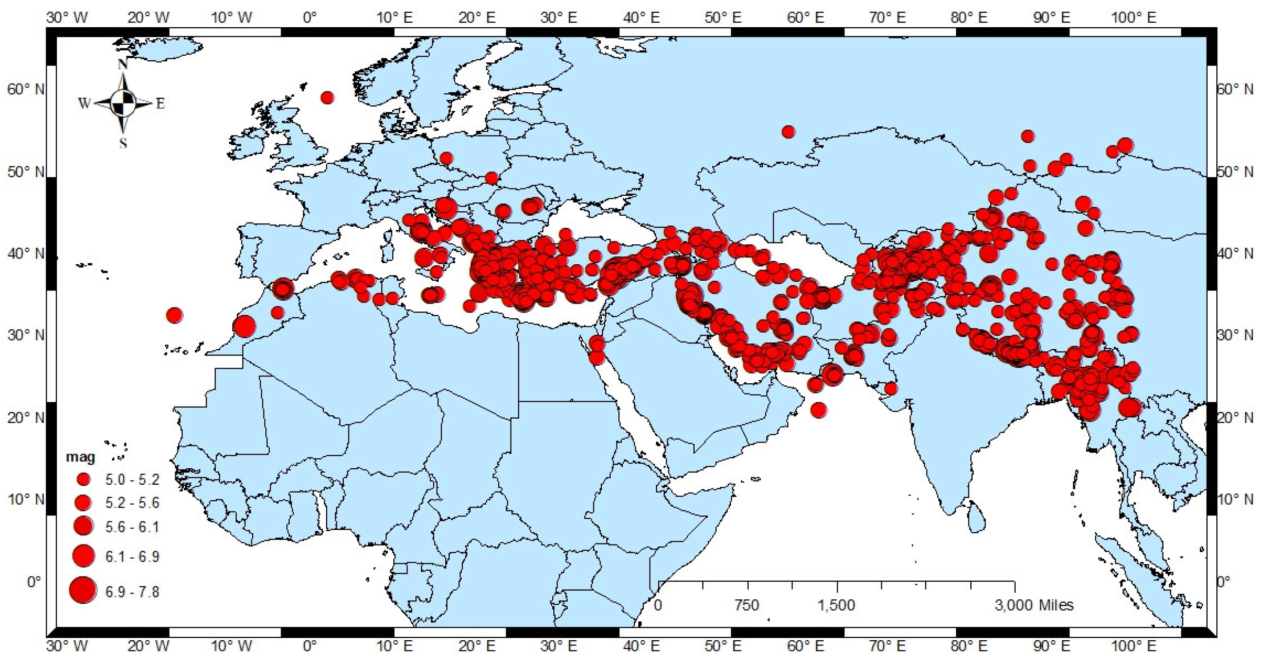
2.1. Swarm Satellite Observations Data
2.2. Seismic Data
2.3. Analysis and Magnetic Field Satellite Anomaly Definition
- The peak-to-peak amplitude is ≥0.3 nT.
- Anomalies should last for at least ten seconds.
- Determine if the anomalies did or did not occur during times when geomagnetic indicators were in quiet conditions.
3. Results and Discussion
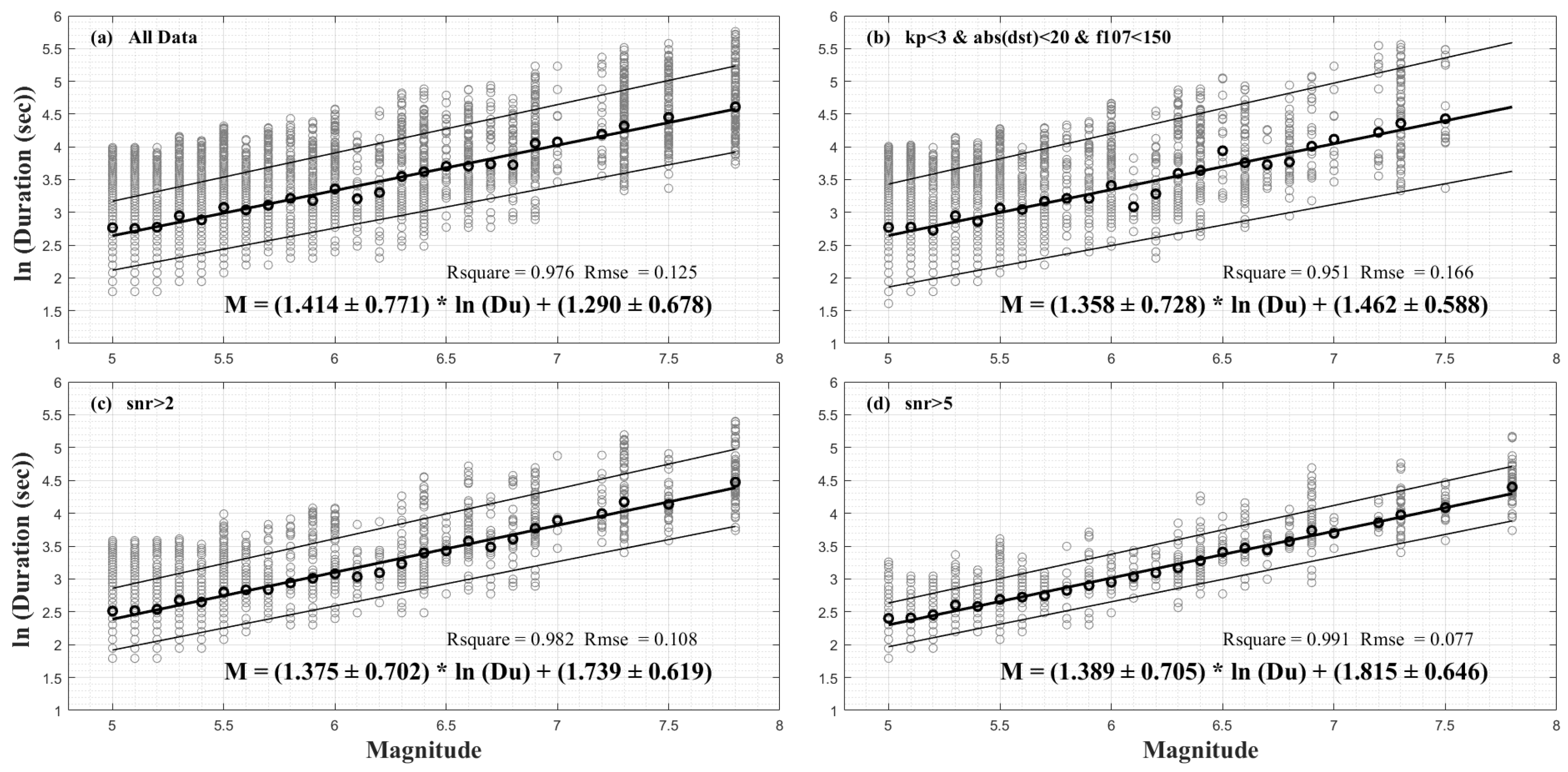
- Magnitude-duration correlation
- Magnitude-Energy correlation
- Magnitude-(Duration × Distance) correlation
- Magnitude-(Duration × Time) correlation
3.1. Confutation Analysis
3.2. Extended Validation Analyses as the Base for an OEPS
4. Conclusions
Supplementary Materials
Author Contributions
Funding
Data Availability Statement
Acknowledgments
Conflicts of Interest
References
- Olaiz, A.J.; Muñoz-Martín, A.; De Vicente, G.; Vegas, R.; Cloetingh, S. European continuous active tectonic strain–stress map. Tectonophysics 2009, 474, 33–40. [Google Scholar] [CrossRef]
- Scholz, C.H. The Mechanics of Earthquakes and Faulting; Cambridge University Press: Cambridge, UK, 2019. [Google Scholar]
- Kanamori, H.; Brodsky, E.E. The physics of earthquakes. Rep. Prog. Phys. 2004, 67, 1429. [Google Scholar] [CrossRef]
- Picozza, P.; Conti, L.; Sotgiu, A. Looking for earthquake precursors from space: A critical review. Front. Earth Sci. 2021, 9, 578. [Google Scholar] [CrossRef]
- Donner, R.V.; Potirakis, S.M.; Balasis, G.; Eftaxias, K.; Kurths, J. Temporal correlation patterns in pre-seismic electromagnetic emissions reveal distinct complexity profiles prior to major earthquakes. Phys. Chem. Earth Parts A/B/C 2015, 85, 44–55. [Google Scholar] [CrossRef]
- Fraser-Smith, A.C.; Bernardi, A.; McGill, P.R.; Ladd, M.; Helliwell, R.; Villard, O.G., Jr. Low-frequency magnetic field measurements near the epicenter of the Ms 7.1 Loma Prieta earthquake. Geophys. Res. Lett. 1990, 17, 1465–1468. [Google Scholar] [CrossRef]
- Gaffet, S.; Guglielmi, Y.; Virieux, J.; Waysand, G.; Chwala, A.; Stolz, R.; Emblanch, C.; Auguste, M.; Boyer, D.; Cavaillou, A. Simultaneous seismic and magnetic measurements in the Low-Noise Underground Laboratory (LSBB) of Rustrel, France, during the 2001 January 26 Indian earthquake. Geophys. J. Int. 2003, 155, 981–990. [Google Scholar] [CrossRef]
- Molchanov, O.A.; Kopytenko, Y.A.; Voronov, P.M.; Kopytenko, E.A.; Matiashvili, T.G.; Fraser-Smith, A.C.; Bernardi, A. Results of ULF magnetic field measurements near the epicenters of the Spitak (Ms = 6.9) and Loma Prieta (Ms = 7.1) earthquakes: Comparative analysis. Geophys. Res. Lett. 1992, 19, 1495–1498. [Google Scholar] [CrossRef]
- Varotsos, P.A. The Physics of Seismic Electric Signals; TerraPub: Tokyo, Japan, 2005; 338p. [Google Scholar]
- Uyeda, S.; Nagao, T.; Kamogawa, M. Short-term earthquake prediction: Current status of seismo-electromagnetics. Tectonophysics 2009, 470, 205–213. [Google Scholar] [CrossRef]
- Hayakawa, M.; Kawate, R.; Molchanov, O.A.; Yumoto, K. Results of ultra-low-frequency magnetic field measurements during the Guam earthquake of 8 August 1993. Geophys. Res. Lett. 1996, 23, 241–244. [Google Scholar] [CrossRef]
- Larkina, V.I.; Nalivayko, A.V.; Gershenzon, N.I.; Gokhberg, M.B.; Liperovskiy, V.A.; Shalimov, S.L. Observations of VLF emission, related with seismic activity, on the Interkosmos-19 satellite. Geomagn. Aeron. 1983, 23, 684. [Google Scholar]
- Parrot, M. Use of satellites to detect seismo-electromagnetic effects. Adv. Sp. Res. 1995, 15, 27–35. [Google Scholar] [CrossRef]
- Balasis, G.; Mandea, M. Can electromagnetic disturbances related to the recent great earthquakes be detected by satellite magnetometers? Tectonophysics 2007, 431, 173–195. [Google Scholar] [CrossRef]
- Ryu, K.; Chae, J.-S.; Lee, E.; Parrot, M. Fluctuations in the ionosphere related to Honshu Twin Large Earthquakes of September 2004 observed by the DEMETER and CHAMP satellites. J. Atmos. Sol. Terr. Phys. 2014, 121, 110–122. [Google Scholar] [CrossRef]
- De Santis, A.; Marchetti, D.; Spogli, L.; Cianchini, G.; Pavón-Carrasco, F.J.; Franceschi, G.D.; Di Giovambattista, R.; Perrone, L.; Qamili, E.; Cesaroni, C.; et al. Magnetic field and electron density data analysis from Swarm satellites searching for ionospheric effects by great earthquakes: 12 Case studies from 2014 to 2016. Atmosphere 2019, 10, 371. [Google Scholar] [CrossRef]
- Varotsos, P.; Sarlis, N.; Skordas, E. Magnetic field variations associated with the SES before the 6.6 Grevena-Kozani Earthquake. Proc. Jpn. Acad. Ser. Β 2001, 77, 93–97. [Google Scholar] [CrossRef]
- Cicerone, R.D.; Ebel, J.E.; Britton, J. A systematic compilation of earthquake precursors. Tectonophysics 2009, 476, 371–396. [Google Scholar] [CrossRef]
- De Santis, A.; Cianchini, G.; Marchetti, D.; Piscini, A.; Sabbagh, D.; Perrone, L.; Campuzano, S.A.; Inan, S. A multiparametric approach to study the preparation phase of the 2019 M7. 1 Ridgecrest (California, United States) earthquake. Front. Earth Sci. 2020, 8, 540398. [Google Scholar] [CrossRef]
- Freund, F. Pre-earthquake signals: Underlying physical processes. J. Asian Earth Sci. 2011, 41, 383–400. [Google Scholar] [CrossRef]
- De Santis, A.; De Franceschi, G.; Spogli, L.; Perrone, L.; Alfonsi, L.; Qamili, E.; Cianchini, G.; Di Giovambattista, R.; Salvi, S.; Filippi, E.; et al. Geospace perturbations induced by the Earth: The state of the art and future trends. Phys. Chem. Earth Parts A/B/C 2015, 85, 17–33. [Google Scholar] [CrossRef]
- Breiner, S. Piezomagnetic effect at the time of local earthquakes. Nature 1964, 202, 790–791. [Google Scholar] [CrossRef]
- Moore, G.W. Magnetic disturbances preceding the 1964 Alaska earthquake. Nature 1964, 203, 508–509. [Google Scholar] [CrossRef]
- Stacey, F.D. Seismo-magnetic effect and the possibility of forecasting earthquakes. Nature 1963, 200, 1083–1085. [Google Scholar] [CrossRef]
- Johnston, M.J.S. Review of electric and magnetic fields accompanying seismic and volcanic activity. Surv. Geophys. 1997, 18, 441–476. [Google Scholar] [CrossRef]
- Zlotnicki, J.; Nishida, Y. Review on morphological insights of self-potential anomalies on volcanoes. Surv. Geophys. 2003, 24, 291–338. [Google Scholar] [CrossRef]
- Freund, F. Earthquake forewarning—A multidisciplinary challenge from the ground up to space. Acta Geophys. 2013, 61, 775–807. [Google Scholar] [CrossRef]
- Hayakawa, M.; Asano, T.; Rozhnoi, A.; Solovieva, M. Very-low-to low-frequency sounding of ionospheric perturbations and possible association with earthquakes. Pre-Earthq. Process. A Multidiscip. Approach Earthq. Predict. Stud. 2018, 275–304. [Google Scholar] [CrossRef]
- Pulinets, S.; Ouzounov, D. Lithosphere–Atmosphere–Ionosphere Coupling (LAIC) model–An unified concept for earthquake precursors validation. J. Asian Earth Sci. 2011, 41, 371–382. [Google Scholar] [CrossRef]
- Friis-Christensen, E.; Lühr, H.; Hulot, G. Swarm: A constellation to study the Earth’s magnetic field. Earth Planets Sp. 2006, 58, 351–358. [Google Scholar] [CrossRef]
- Ritter, P.; Lühr, H.; Rauberg, J. Determining field-aligned currents with the Swarm constellation mission. Earth Planets Sp. 2013, 65, 1285–1294. [Google Scholar] [CrossRef]
- Olsen, N.; Friis-Christensen, E.; Floberghagen, R.; Alken, P.; Beggan, C.D.; Chulliat, A.; Doornbos, E.; Da Encarnação, J.T.; Hamilton, B.; Hulot, G.; et al. The Swarm satellite constellation application and research facility (SCARF) and Swarm data products. Earth Planets Sp. 2013, 65, 1189–1200. [Google Scholar] [CrossRef]
- Olsen, N.; Ravat, D.; Finlay, C.C.; Kother, L.K. LCS-1: A high-resolution global model of the lithospheric magnetic field derived from CHAMP and Swarm satellite observations. Geophys. J. Int. 2017, 211, 1461–1477. [Google Scholar] [CrossRef]
- Grayver, A.V.; Schnepf, N.R.; Kuvshinov, A.V.; Sabaka, T.J.; Manoj, C.; Olsen, N. Satellite tidal magnetic signals constrain oceanic lithosphere-asthenosphere boundary. Sci. Adv. 2016, 2, e1600798. [Google Scholar] [CrossRef] [PubMed]
- Irrgang, C.; Saynisch, J.; Thomas, M. Utilizing oceanic electromagnetic induction to constrain an ocean general circulation model: A data assimilation twin experiment. J. Adv. Model. Earth Syst. 2017, 9, 1703–1720. [Google Scholar] [CrossRef]
- De Santis, A.; Marchetti, D.; Pavón-Carrasco, F.J.; Cianchini, G.; Perrone, L.; Abbattista, C.; Alfonsi, L.; Amoruso, L.; Campuzano, S.A.; Carbone, M.; et al. Precursory worldwide signatures of earthquake occurrences on Swarm satellite data. Sci. Rep. 2019, 9, 20287. [Google Scholar] [CrossRef] [PubMed]
- Rikitake, T. Earthquake precursors in Japan: Precursor time and detectability. Tectonophysics 1987, 136, 265–282. [Google Scholar] [CrossRef]
- Dobrovolsky, I.P.; Zubkov, S.I.; Miachkin, V.I. Estimation of the size of earthquake preparation zones. Pure Appl. Geophys. 1979, 117, 1025–1044. [Google Scholar] [CrossRef]
- Yan, R.; Parrot, M.; Pinçon, J.-L. Statistical Study on Variations of the Ionospheric Ion Density Observed by DEMETER and Related to Seismic Activities. J. Geophys. Res. Space Phys. 2017, 122, 12–421. [Google Scholar] [CrossRef]
- Plastino, W.; Bella, F.; Catalano, P.G.; Di Giovambattista, R. Radon groundwater anomalies related to the Umbria-Marche, September 26, 1997, earthquakes. Geofis. Int. 2002, 41, 369–375. [Google Scholar]
- Vizzini, F.; Brai, M. In-soil radon anomalies as precursors of earthquakes: A case study in the SE slope of Mt. Etna in a period of quite stable weather conditions. J. Environ. Radioact. 2012, 113, 131–141. [Google Scholar] [CrossRef] [PubMed]
- De Santis, A.; Balasis, G.; Pavòn-Carrasco, F.J.; Cianchini, G.; Mandea, M. Potential earthquake precursory pattern from space: The 2015 Nepal event as seen by magnetic Swarm satellites. Earth Planet. Sci. Lett. 2017, 461, 119–126. [Google Scholar] [CrossRef]
- Trnkoczy, A. Understanding & setting sta/lta trigger algorithm parameters for the k2. Appl. Note 1998, 41, 16–20. [Google Scholar]
- Riswadkar, A.V.; Dobbins, B. Solar Storms: Protecting Your Operations Against the Sun’s’ Dark Side. Zurich Serv. Corp. Schaumbg. 2010, 1–12. Available online: https://www.nuevatribuna.es/media/nuevatribuna/files/2014/02/06/solarstorms.pdf (accessed on 1 February 2024).
- Zerbo, J.L.; Amory Mazaudier, C.; Quattara, F.; Richardson, J.D. Solar wind and geomagnetism: Toward a standard classification of geomagnetic activity from 1868 to 2009. Ann. Geophys. 2012, 20, 421–426. [Google Scholar] [CrossRef]
- Pulinets, S.; Boyarchuk, K. Ionospheric Precursors of Earthquakes; Springer Science & Business Media: Berlin/Heidelberg, Germany, 2004. [Google Scholar]
- Marchetti, D.; De Santis, A.; Campuzano, S.A.; Soldani, M.; Piscini, A.; Sabbagh, D.; Cianchini, G.; Perrone, L.; Orlando, M. Swarm Satellite Magnetic Field Data Analysis Prior to 2019 Mw = 7.1 Ridgecrest (California, USA) Earthquake. Geosciences 2020, 10, 502. [Google Scholar] [CrossRef]
- Pinheiro, K.J.; Jackson, A.; Finlay, C.C. Measurements and uncertainties of the occurrence time of the 1969, 1978, 1991, and 1999 geomagnetic jerks. Geochem. Geophys. Geosystems 2011, 12, 32. [Google Scholar] [CrossRef]
- De Santis, A.; Perrone, L.; Calcara, M.; Campuzano, S.A.; Cianchini, G.; D’Arcangelo, S.; Di Mauro, D.; Marchetti, D.; Nardi, A.; Orlando, M.; et al. A comprehensive multiparametric and multilayer approach to study the preparation phase of large earthquakes from ground to space: The case study of the June 15 2019, M7. 2 Kermadec Islands (New Zealand) earthquake. Remote Sens. Environ. 2022, 283, 113325. [Google Scholar] [CrossRef]
- Namgaladze, A.A.; Klimenko, M.V.; Klimenko, V.V.; Zakharenkova, I.E. Physical mechanism and mathematical modeling of earthquake ionospheric precursors registered in total electron content. Geomagn. Aeron. 2009, 49, 252–262. [Google Scholar] [CrossRef]
- Pulinets, S.; Ouzounov, D.; Parrot, M. Conjugated near-equatorial effects registered by DEMETER satellite before Sumatra earthquake M8. 7 of March 28, 2005. J. Asian Earth Sci. 2006, 49, 252–262. [Google Scholar]
- Yeturu, K. Chapter 3—Machine learning algorithms, applications, and practices in data science. In Handbook of Statistics; Rao, A.S.R.S., Rao, C.R., Eds.; Elsevier: Amsterdam, The Netherlands, 2020; Volume 43, pp. 81–206. [Google Scholar] [CrossRef]
- Saad, O.M.; Chen, Y.; Savvaidis, A.; Fomel, S.; Jiang, X.; Huang, D.; Oboué, Y.A.; Yong, S.; Wang, X.A.; Zhang, X.; et al. Earthquake Forecasting Using Big Data and Artificial Intelligence: A 30-Week Real-Time Case Study in China. Bull. Seismol. Soc. Am. 2023, 113, 2461–2478. [Google Scholar] [CrossRef]
- Swets, J.A.; Dawes, R.M.; Monahan, J. Better decisions through science. Sci. Am. 2000, 283, 82–87. Available online: https://www.jstor.org/stable/26058901 (accessed on 1 February 2024). [CrossRef] [PubMed]
- Sarlis, N.V. Statistical Significance of Earth’s Electric and Magnetic Field Variations Preceding Earthquakes in Greece and Japan Revisited. Entropy 2018, 20, 561. [Google Scholar] [CrossRef]


| Magnitude Range | Number of EQs That Exhibit Anomalies | Total Number of EQs | Percentage (%) |
|---|---|---|---|
| Full range | 900 | 1077 | 83.5 |
| 5.0–5.5 | 663 | 821 | 80.8 |
| 5.5–6.0 | 155 | 172 | 90 |
| 6.0–6.5 | 53 | 55 | 96 |
| 6.5–7.8 | 29 | 29 | 100 |
| Magnitude Range | Number of EQs That Exhibit Anomalies | Total Number of EQs | Percentage (%) |
|---|---|---|---|
| Full range | 615 | 786 | 78.2 |
| 5.0–5.5 | 448 | 594 | 75.4 |
| 5.5–6.0 | 110 | 130 | 84.6 |
| 6.0–6.5 | 38 | 43 | 88.3 |
| 6.5–7.8 | 19 | 19 | 100 |
| Zone | Number of EQs That Exhibit Anomalies | Total Number of EQs | Percentage (%) |
|---|---|---|---|
| Base | 900 | 1076 | 83 |
| Shift | 256 | 1069 | 24 |
| Zone | Number of EQs That Exhibit Anomalies | Total Number of EQs | Percentage (%) |
|---|---|---|---|
| Base | 615 | 786 | 78 |
| Shift | 132 | 770 | 17 |
| Bx, By, Bz Anomalies | Seismicity | |
|---|---|---|
| Y | N | |
| Y | 5699 | 800 |
| N | 1126 | 1427 |
| Column totals | 6825 | 2227 |
Disclaimer/Publisher’s Note: The statements, opinions and data contained in all publications are solely those of the individual author(s) and contributor(s) and not of MDPI and/or the editor(s). MDPI and/or the editor(s) disclaim responsibility for any injury to people or property resulting from any ideas, methods, instructions or products referred to in the content. |
© 2024 by the authors. Licensee MDPI, Basel, Switzerland. This article is an open access article distributed under the terms and conditions of the Creative Commons Attribution (CC BY) license (https://creativecommons.org/licenses/by/4.0/).
Share and Cite
Alimoradi, H.; Rahimi, H.; De Santis, A. Successful Tests on Detecting Pre-Earthquake Magnetic Field Signals from Space. Remote Sens. 2024, 16, 2985. https://doi.org/10.3390/rs16162985
Alimoradi H, Rahimi H, De Santis A. Successful Tests on Detecting Pre-Earthquake Magnetic Field Signals from Space. Remote Sensing. 2024; 16(16):2985. https://doi.org/10.3390/rs16162985
Chicago/Turabian StyleAlimoradi, Homayoon, Habib Rahimi, and Angelo De Santis. 2024. "Successful Tests on Detecting Pre-Earthquake Magnetic Field Signals from Space" Remote Sensing 16, no. 16: 2985. https://doi.org/10.3390/rs16162985
APA StyleAlimoradi, H., Rahimi, H., & De Santis, A. (2024). Successful Tests on Detecting Pre-Earthquake Magnetic Field Signals from Space. Remote Sensing, 16(16), 2985. https://doi.org/10.3390/rs16162985