Underwater Acoustic Scattering from Multiple Ice Balls at the Ice–Water Interface

Abstract

We investigate the underwater acoustic scattering from various distributed “ice balls” floating on the water, aiming to understand acoustic scattering in the marginal ice zone (MIZ). The MIZ, including a wide range of heterogeneous ice cover, significantly impacts acoustic propagation. We use acoustic modelling, simulation, and laboratory experiments to understand the acoustic scattering from various distributed ice balls. The acoustic scattering fields from a single sound source (90 kHz) in water are analyzed based on selected principal scattering waves between the surfaces of ice and water. The target strengths are calculated using the plate element method and physical acoustic methods, which are validated with water tank experimental data. The methodology is then extended to multiple ice ball cases, specifically considering a single ice ball, equally spaced ice balls of the same size, and randomly distributed ice balls of various sizes. Additionally, experimental measurements under similar conditions are conducted in a laboratory water tank. The scattering intensities at different receiving positions are simulated and compared with lab experiments. The results show good agreement between experimental and numerical results, with an absolute error of less than 3 dB. Scattering intensity is positively correlated with water surface reflection when the receiving angle is close to the mirror reflection angle of the incident wave. Our approach sets the groundwork for further research to address more complex ice–water interfaces with various ice covers in the MIZ.

1. Introduction

Remote sensing technology is widely applied across various fields, yet single-source remote sensing is no longer sufficient to meet the information acquisition needs in complex environments. Consequently, multi-source information fusion technology gradually became a research hotspot. In polar regions, the transmission of radio and light waves in water is limited, making acoustic waves the primary medium for information transmission. For instance, the propagation distance of light waves in water is limited, typically penetrating only a few meters deep, while radio waves attenuate rapidly in water, rendering them nearly ineffective for transmitting information. Therefore, acoustic waves, with their advantages of long propagation distance and lower attenuation in water, became the main medium for underwater information sensing and transmission in polar regions. Research vessels operating in polar oceans often utilize sonar systems to transmit sound waves for underwater communication and detection. The presence of sea ice cover can scatter and absorb the acoustic waves propagating underneath, thus reducing the efficiency of related work. It is critical to understand the scattering mechanisms of sound waves in the marginal ice zone (MIZ) for ensuring the safety of navigation and other operations in the polar regions. Therefore, continuous attention in Arctic hydroacoustic research is demanded for hydroacoustic studies to elucidate the acoustic scattering characteristics at the ice–water boundary and to unravel the complexities of the scattering processes related to the sea ice [1].

Hutt [2] provided a comprehensive review of the underwater acoustic field, emphasizing how the presence of ice cover significantly influences acoustic properties. This foundational understanding led to the development of underwater acoustic techniques for detecting ice cover, which are crucial for improving acoustic communication and navigation beneath sea ice [3,4,5]. McCammom et al. [6] built upon this by modeling an ice layer as a continuous elastic medium to calculate the reflection coefficient of a layered elastic solid plane wave. Their model, which assumes a fluid half space, offers insights into the relationship between the internal properties of ice and the acoustic reflection at the ice–water interface. Extending this work, Liu et al. [7] analyzed the scattering coefficient and coherent reflection from a rough, single-layer sea ice cover, highlighting the complexities of acoustic interactions in such environments.

While these studies focus on continuous ice layers, the marginal ice zone (MIZ) presents unique challenges due to the diverse forms of sea ice, such as frazil ice, grease ice, and pancake ice. To address these challenges, several studies from difference aspects are briefly reviewed. Lucieer et al. [8] introduced novel multiple workflows for processing underwater acoustic bathymetry and backscatter data. Their approach can identify distinct sea ice textures, providing new insights into the acoustic signatures of various ice surfaces. In parallel, Jiang et al. [9] developed a semi-supervised interactive system for classifying sea ice in dual-polarized RADARSAT-2 imagery. This system leverages machine learning techniques to handle the increasing volume of SAR data, offering a complementary approach to traditional manual interpretation. Empirical observations by Garrison et al. [10] and Ito et al. [11] provide further insights into acoustic scattering in icy environments. Garrison et al. measured the backscattering intensity from the bottom of flat, one-year sea ice using a 60 kHz pulse signal, contributing valuable data on acoustic interactions with older, stable ice. Ito et al. focused on detecting backscatter signals from underwater frazil ice and sediment using bottom-mounted acoustic Doppler current profilers with a 300 kHz frequency, shedding light on the acoustic properties in more dynamic ice conditions.

It is a challenge to model the underwater acoustic scattering field beneath partially ice-covered water. Acoustic waves near the ice–water boundary give rises to a multiple-scattered acoustic field due to repeated reflections from the water surface and submerged ice. Accordingly, the problem of sound scattering with at the ice–water interface can be considered as an extension of the target sound scattering problem at the interface, a topic receiving considerable attention. Huang and Gaunaurd [12,13] used a classical separation of variables technique to precisely analyze the acoustic scattering by a submerged spherical elastic shell near a free surface, ensuring the boundary conditions on the shell and free surface were satisfied. A virtual source method was employed to examine the acoustic scattering of plane waves around spherical objects at various incident angles within low to medium frequency ranges, where the acoustic scattering fields are solved by expanding the classical modal series of the spherical wave function. The authors further studied the sound scattering by bubble clouds near the sea surface, adapting the classical formulation for evaluating the scattering cross-sections of a single air bubble in a liquid, to a cloud of interacting bubbles near a boundary. The adaption resulted in multiple scattering cross-sections and a series of coupled algebraic equations to determine the coupling coefficients [14]. Richardson et al. [15] studied the scattering of high-frequency acoustic signal scattering from seashells to model seafloor backscattering. They conducted experiments on varying sizes of glass beads and shells. Comparison of the measurements with a simple target strength-based model’s predication indicated the potential importance of interface and multiple scattering effects, and the discrete scatterers in backscattering scenarios. Kungl et al. [16] expanded the theoretical framework by modeling frazil ice in open water as both a sphere and an oblate spheroid. Their work extended the classical Rayleigh analysis to determine the acoustic backscattering cross-section. Their oblate spheroid-based backscattering model is consistent with previous laboratory studies and observations of frazil ice in rivers across a broad frequency range from 125 kHz to 774 kHz.

Furthermore, advanced numerical methods were developed to resolve scattering problems with complicated target surfaces. Simon et al. [17] adopted the finite element method to model acoustic wave propagation scattered by the ice–water interface, where the ice cover is modeled as both an elastic medium and a pressure release surface. Chen et al. [18] proposed a boundary condition method for calculating the acoustic reflection coefficient of the layered ice–snow model based on the conditions between two adjacent layers. The plate element method is used to model complex interface shape and calculate the scattering field of the target with an incident plane wave [19,20]. Abewi [21] modeled a target as an assembly of triangular facets to solve the scattering problem from a target in a waveguide. The Kirchhoff approximation was used to compute scattering from each facet analytically for each set of incident and scattered plane waves, and solutions were then combined coherently.

This study focuses on the impact of polar sea ice surfaces on underwater acoustic wave propagation, aiming to enhance the accuracy of underwater information sensing and transmission and to provide theoretical support for the application of multi-source information fusion technology in polar environments. Specifically, this paper examines the acoustic scattering phenomena due to partial sea ice coverage in the MIZ, particularly brash ice, with notable three-dimensional shapes. For analytical tractability, following Kungl et al. [16], we simplify the complex ice–water interface by treating individual ice floes as spherical scatterers with acoustic resistance, hereafter called ice balls. This approach enables a detailed analysis of the principal scattering waves and provides insights into the acoustic field under rough interface. This simplification inherently limits the model’s ability to capture the irregular geometries, and variable surface roughness of various ice types will, consequently, not be fully represented in the real MIZ. Nonetheless, this approach provides a necessary foundation for extending the analysis to more complex and realistic ice–water interfaces. We further extend this model to account for multiple, randomly distributed ice balls and explore both uniform and non-uniform distributions. This comprehensive analysis is crucial for understanding the acoustic behavior in real MIZ conditions, where ice floes are rarely uniform. The theoretical models are then validated through controlled water tank experiments, with results showing good agreement between simulated and experimental data, reinforcing the reliability of the proposed models. These findings have direct implications for acoustic detection and communication in polar regions, laying the groundwork for future research and operational strategies in these challenging environments.

The structure of this paper is addressed below. In Section 2, we investigate the sound scattering of a spherical ball floating in the water. By accounting for principal scattering paths, the acoustic scattering field of an ice–water interface is simulated using the plate element method. Moreover, we conduct acoustic scattering experiments with real ice balls in a water tank for validation. In Section 3, the model is further extended for general conditions, including multiple ice balls with different sizes, and to report the relevant validations by laboratory experiments. The discussion and conclusion are given in Section 4.

2. Single Ice Ball Model

For an inelastic target, the acoustic scattering field is primarily governed by the geometric shape of the target surface, while the surface impedance characteristics can be treated as a geometric scattering field. In the case of high-frequency waves (i.e., $ka>>1$, where $k$ indicates the wavenumber, and a indicates the radius of the ice ball) [22], the scattered waves are inclined to follow the patterns of geometric scattering. In fact, geometrically scattered waves often form the essence of an acoustic scattering field. Given that the surface of an ice ball is non-rigid, the resulting acoustic scattering field contains both internal elastic echoes and geometric reflections. Our focus primarily lies on geometric scattering, and an additional reflection coefficient attributable to the resistive surface of an ice ball. This reflection coefficient is influenced by the angle and frequency of the incident wave, and the properties of the ice surface.

The plate element method is utilized to calculate the surface element integral of complex target surfaces. By applying Green’s theorem, the area integral of acoustic scattering by a target surface is transformed into a line integral, subsequently simplified as a simple algebraic summation. For each small surface element, its acoustic scattering field is solvable through classical acoustic methods. The aggregate acoustic scattering field is represented by the vector summation of the acoustic fields emanating from all elements. Hence, the plate element method is appropriate for simulating the underwater acoustic scattering field of intricate targets. The precision of calculation improves with finer element subdivision yet incurs higher computational costs.

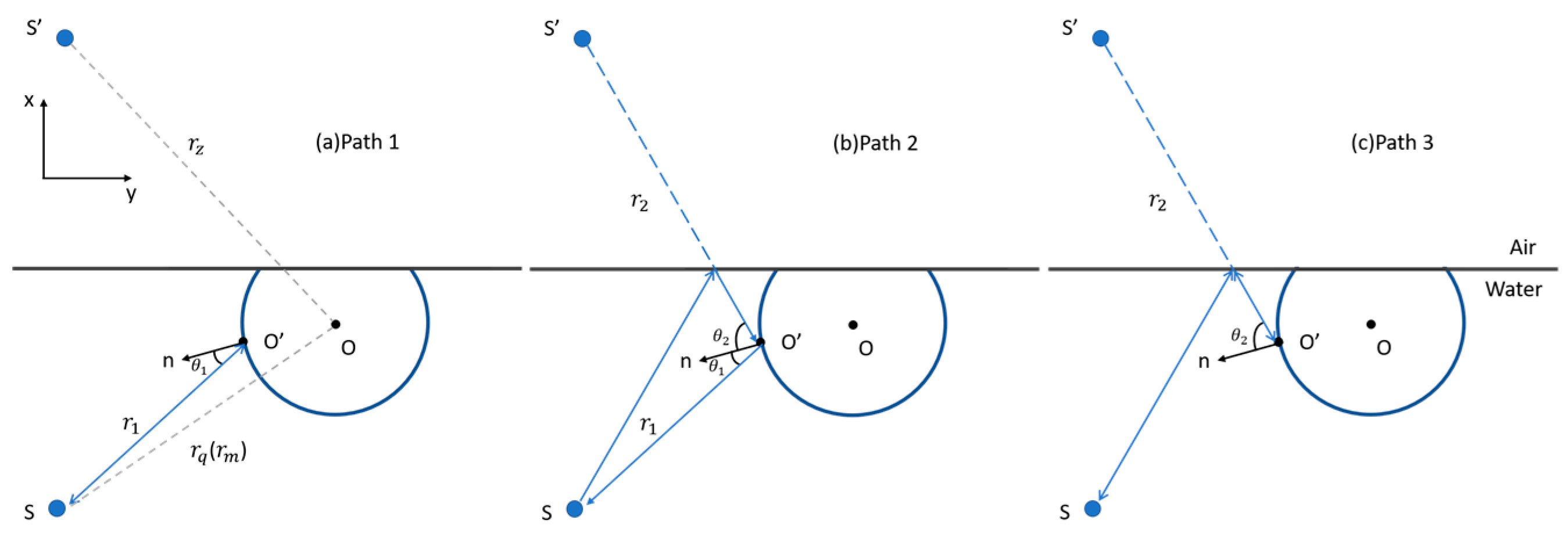
2.1. Acoustic Scattering under Ice–Water Interface with a Single Ice Ball

The acoustic scattering field for an ice ball floating on water is more complex than that in the free field. This complexity comes from multiple scatterings between the target and the water surface, resulting in a complicated echo structure of acoustic scattering around the target, which in turns influences the target strength. The Kirchhoff approximation formula for the target scattering problem near the interface [23,24] is discussed further below,

$${\varphi }_s\left(\mathit{r}\right)={\displaystyle \frac{1}{4\pi }}{\iint }_s\left[{\varphi }_s\right(Q){\displaystyle \frac{\partial G(\mathit{r},Q)}{\partial \mathit{n}}}-G(\mathit{r},Q\left){\displaystyle \frac{\partial {\varphi }_s\left(Q\right)}{\partial \mathit{n}}}\right]ds$$

(1)

where ${\varphi }_s\left(\mathit{r}\right)$ is the scattering potential function at the receiving point $R$ in the semi-infinite space with vector radius $\mathit{r}$, $\mathit{n}$ is the outer normal direction, ${\varphi }_s\left(Q\right)$ is the potential function at the scattering point $Q$ on the surface, and $G(\mathit{r},Q)$ is an approximation of the Green’s function in the semi-infinite space:

$$G(r_2,Q)={\displaystyle \frac{e^{jk{r}_1}}{r_1}}+V_b\left(\alpha \right){\displaystyle \frac{e^{jk{r}_2}}{r_2}}$$

(2)

where $j$ indicates imaginary unit, $V_b\left(\alpha \right)$ is reflection coefficient of the interface, $\alpha$ is the included angle between the incident wave direction and the interface normal direction, $r_1$ indicates distance from the sound source $S$ to $Q$, and $r_2$ indicates distance from the virtual source $S^{\prime }$ of $S$ to $Q$.

For the condition of monostatic transducer, the potential function of incident acoustic wave ${\varphi }_i$ consists of the direct wave and the interface reflected wave, which shares the same format as the Green’s function in Equation (2):

$${\varphi }_i\left(Q\right)={\displaystyle \frac{e^{jk{r}_1}}{r_1}}+V_b\left(\alpha \right){\displaystyle \frac{e^{jk{r}_2}}{r_2}}.$$

(3)

For targets with a non-rigid surface, such as the ice discussed in this paper, in the case of high frequencies where the local plane wave approximation is applicable ($ka>>1$). We denote the surface reflection coefficient as V(β) and the acoustic impedance as $Z_b$. The following equations describe the behavior at the target surface:

$$\left\{\begin{array}{c}{\varphi }_s=V\left(\beta \right){\displaystyle \frac{e^{jk{r}_1}}{r_1}}+V\left(\beta \right)V_b\left(\alpha \right){\displaystyle \frac{e^{jk{r}_2}}{r_2}}\\ {\displaystyle \frac{j\omega \rho \left({\mathsf{\varphi }}_i+{\mathsf{\varphi }}_s\right)}{\partial \left({\mathsf{\varphi }}_i+{\mathsf{\varphi }}_s\right)/\partial n}}=-Z_b\end{array}\right..$$

(4)

We have an approximation under far-field condition:

$${\displaystyle \frac{\partial G}{\partial n}}={\displaystyle \frac{\partial {\varphi }_i}{\partial n}}=-jk\left[{\displaystyle \frac{e^{jk{r}_1}}{r_1}}\mathit{cos}{\theta }_1+V_b\left(\alpha \right){\displaystyle \frac{e^{jk{r}_2}}{r_2}}\mathit{cos}{\theta }_2\right]$$

(5)

where $\mathit{cos}{\theta }_1=\partial r_1/\partial n$ and $\mathit{cos}{\theta }_2=\partial r_2/\partial n$. Substituting Equation (4) into Equation (5), we can obtain

$$-{\displaystyle \frac{\partial {\varphi }_s}{\partial n}}=\left[{\displaystyle \frac{jk\rho c}{Z_b}}\left(1+V\left(\beta \right)\right)-jk\cos {\theta }_1\right]{\displaystyle \frac{e^{jk{r}_1}}{r_1}}+\left[{\displaystyle \frac{jk\rho c}{Z_b}}\left(1+V\left(\beta \right)\right)V_b\left(\alpha \right)-jk{V}_b\left(\alpha \right)\cos {\theta }_2\right]{\displaystyle \frac{e^{jk{r}_2}}{r_2}}.$$

(6)

Substituting Equations (5) and (6) into Equation (1), and considering the relationship: ${\displaystyle \frac{1-V\left(\beta \right)}{1+V\left(\beta \right)}}={\displaystyle \frac{\rho c/\mathit{cos}{\theta }_1}{Z_b}}$, where $\rho$ is water density and $c$ is sound speed in water, it yields the physical acoustic formula of the scattering field beneath the resistive surface target at the water surface as

$${\varphi }_s=-{\displaystyle \frac{jk}{2\pi }}{\iint }_s\left\{V\left(\beta \right)[\cos {\theta }_1{\displaystyle \frac{e^{j2k{r}_1}}{r_1^2}}+\right.V_b\left(\alpha \right)\left(\cos {\theta }_1+\cos {\theta }_2\right)\left.{\displaystyle \frac{e^{jk\left(r_2+r_1\right)}}{r_2{r}_1}}+V_b^2\left(\alpha \right)\cos {\theta }_2{\displaystyle \frac{e^{j2k{r}_2}}{r_2^2}}]\right\}dS.$$

(7)

The surfaces of the target and water can be discretized into a number of small elements M using the plate element method. This approach enables us to effectively approximate the integral of the acoustic scattering problem. As the number of plate elements M approaches infinity, the scattering potential function can be written as

$${\varphi }_s=\underset{M\to \infty }{\lim }{\sum }_{m=1}^M{\left({\phi }_{s1}+{\phi }_{s2}+{\phi }_{s3}\right)}_m.$$

(8)

For the single ice ball model with a monostatic transducer, we select three principal scattering paths for sound waves emanating from source S. The choice of these paths is detailed below and is depicted in Figure 1 to help visualize each path.

• Path 1: A sound wave from S is reflected off the ice ball’s spherical surface and returns to S. This trajectory represents the target echo in the free field, unaffected by the water surface, and is commonly considered as the primary contributor to the overall acoustic scattering field [22,25].
• Path 2: A sound wave from S initially reaches the water surface, then contacts the target surface following reflection off the water, and then reverberates back to S after the spherical reflection; alternatively, the sound wave from S first reaches the spherical surface of the target, and subsequently the water surface, before finally reaching S. Both trajectories exemplify double-station scattering from S to S’.
• Path 3: A sound wave from S is reflected by the water surface to reach the spherical surface of the ice ball. Subsequently, it is reflected from the spherical surface to the water surface and then back to S. This path represents a single-station echo of S’ relative to the ice ball.

Potential functions corresponding to the selected paths are:

Path 1:

$$({\phi }_{s1}{)}_m=-{\displaystyle \frac{jk}{2\pi }}{\displaystyle \frac{e^{2jk{r}_q}}{{r_q}^2}}\left[{\displaystyle \frac{jk{r}_q-1}{jk{r}_q}}\mathit{cos}{\theta }_1\right]S_{m1}$$

(9)

where $S_{m1}={{\iint }_{\mathsf{\Delta }{S}_{m1}}e}^{-2jk\mathsf{\Delta }{r}_q}ds$.

Path 2:

$$({\phi }_{s2}{)}_m=-{\displaystyle \frac{jk}{2\pi }}{\displaystyle \frac{e^{jk\left(r_q+r_z\right)}}{r_q{r}_z}}{V}_b\left(\alpha \right)\left[{\displaystyle \frac{jk{r}_q-1}{jk{r}_q}}\mathit{cos}{\theta }_1+{\displaystyle \frac{jk{r}_z-1}{jk{r}_z}}\mathit{cos}{\theta }_2\right]{S_m}_2$$

(10)

where $S_{m2}={{\iint }_{\mathsf{\Delta }{S}_{m2}}e}^{-2jk\mathsf{\Delta }{r}_z}ds$.

Path 3:

$$({\phi }_{s3}{)}_m=-{\displaystyle \frac{jk}{2\pi }}{\displaystyle \frac{e^{2jk{r}_z}}{{r_z}^2}}{V_b}^2\left(\alpha \right)\left[{\displaystyle \frac{jk{r}_z-1}{jk{r}_z}}\mathit{cos}{\theta }_2\right]{S_m}_3$$

(11)

where $S_{m3}={{\iint }_{\mathsf{\Delta }{S}_{m3}}e}^{-jk(\mathsf{\Delta }{r}_q+\mathsf{\Delta }{r}_z)}ds$.

In a scenario employed with a bistatic configuration, we present four principal scattering paths, such as the derivation of the scattering potential function under the monostatic transducer. These paths are described below and illustrated in Figure 2.

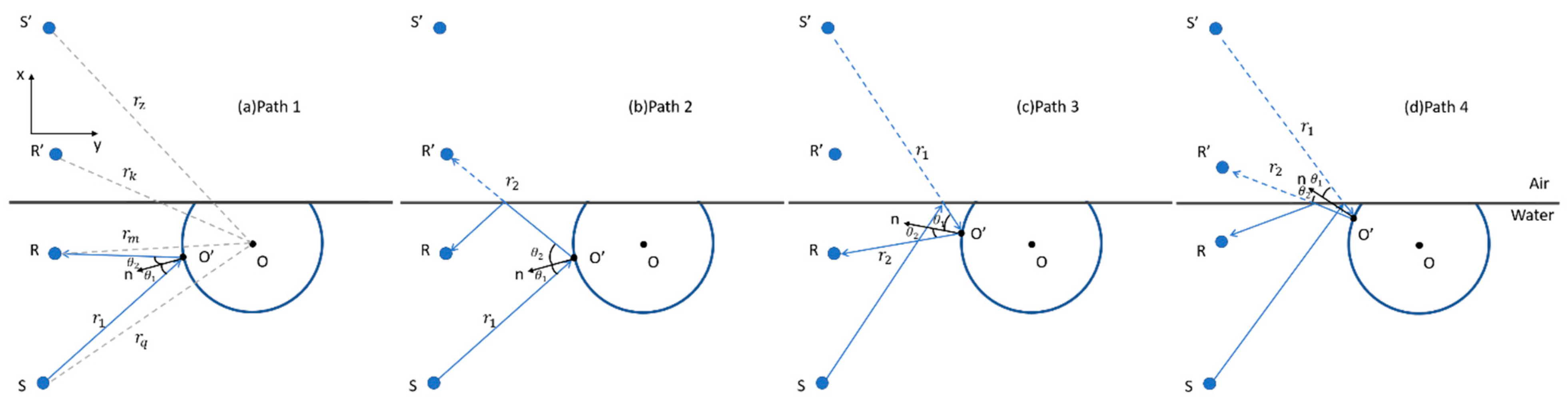
• Path 1: considering the target echo in the free field without interface effect, that is, the sound wave from S reaches R after being reflected by the ice ball.
• Path 2: Starting from S, the wave reaches the ice ball surface, then the water surface, and finally R. This is equivalent to the path arriving at the mirror image point of the receiving position R’ through the water surface. The reflection coefficient $V_b\left(\alpha \right)$ is added due to the reflection at the water surface.
• Path 3: Similar to the path 2, $V_b\left(\alpha \right)$ is considered. The path can be viewed as the starting point at the S’ and reaching R after being reflected by the ice ball surface.
• Path 4: Both the incident and reflected waves from the ice ball are reflected by the water surface, which can be viewed as waves emitted from S’ to R’ after being reflected by the ice ball surface. Due to the twice reflections at the water surface, the interface reflection coefficient becomes a quadratic term $V_b^2\left(\alpha \right)$.

The relevant potential functions of scattering field for the biostatic transducer case:

Path 1:

$$({\phi }_{s1}{)}_m=-{\displaystyle \frac{jk}{4\pi }}{\displaystyle \frac{e^{jk(r_q+r_m)}}{r_q{r}_m}}V(\beta )\left[{\displaystyle \frac{jk{r}_q-1}{jk{r}_q}}\mathit{cos}{\theta }_1+{\displaystyle \frac{jk{r}_m-1}{jk{r}_m}}\mathit{cos}{\theta }_2\right]S_{m1}$$

(12)

where $S_{m1}={{\iint }_{\mathsf{\Delta }{S}_{m1}}e}^{-jk(\mathsf{\Delta }{r}_q+\mathsf{\Delta }{r}_m)}ds$.

Path 2:

$$({\phi }_{s2}{)}_m=-{\displaystyle \frac{jk}{4\pi }}{\displaystyle \frac{e^{jk\left(r_q+r_k\right)}}{r_q{r}_k}}{V}_b\left(\alpha \right)\left[V\left(\beta \right){\displaystyle \frac{(jk{r}_q-1)}{jk{r}_q}}\mathit{cos}{\theta }_1+V\left(\beta \right){\displaystyle \frac{(jk{r}_k-1)}{jk{r}_k}}\mathit{cos}{\theta }_2\right]{S_m}_2$$

(13)

where $S_{m2}={{\iint }_{\mathsf{\Delta }{S}_{m2}}e}^{-jk(\mathsf{\Delta }{r}_q+\mathsf{\Delta }{r}_k)}ds$.

Path 3:

$$({\phi }_{s3}{)}_m=-{\displaystyle \frac{jk}{4\pi }}{\displaystyle \frac{e^{jk\left(r_z+r_m\right)}}{r_z{r}_m}}{V}_b\left(\alpha \right)\left[V\left(\beta \right){\displaystyle \frac{(jk{r}_z-1)}{jk{r}_z}}\mathit{cos}{\theta }_1+V\left(\beta \right){\displaystyle \frac{(jk{r}_m-1)}{jk{r}_m}}\mathit{cos}{\theta }_2\right]{S_m}_3$$

(14)

where $S_{m3}={{\iint }_{\mathsf{\Delta }{S}_{m3}}e}^{-jk(\mathsf{\Delta }{r}_z+\mathsf{\Delta }{r}_m)}ds$.

Path 4:

$$({\phi }_{s4}{)}_m=-{\displaystyle \frac{jk}{4\pi }}{\displaystyle \frac{e^{jk\left(r_z+r_k\right)}}{r_z{r}_k}}{V_b}^2\left(\alpha \right)\left[V\left(\beta \right){\displaystyle \frac{\left(jk{r}_z-1\right)}{jk{r}_z}}\mathit{cos}{\theta }_1+V\left(\beta \right){\displaystyle \frac{\left(jk{r}_k-1\right)}{jk{r}_k}}\mathit{cos}{\theta }_2\right]{S_m}_4$$

(15)

where $S_{m4}={{\iint }_{\mathsf{\Delta }{S}_{m4}}e}^{-jk(\mathsf{\Delta }{r}_z+\mathsf{\Delta }{r}_k)}ds$.

The target strength of an object is defined as

$$TS=10\log {\left|{\displaystyle \frac{I_r}{I_i}}\right|}_{r=1m}$$

(16)

where $I_i$ indicates the incident sound intensity at the object, and $I_r$ indicates the scattered sound intensity at $r=1 \mathrm{m}$ from the center of the object. We can rewrite Equation (16) in terms of the potential function as:

$$TS=20\log {\left|{\displaystyle \frac{r·{\varphi }_s}{{\varphi }_i}}\right|}_{r=1\mathrm{m}}.$$

(17)

Substituting the principal potential functions mentioned above into Equation (17), we can obtain the target strength in the acoustic scattering field of a single ice ball model.

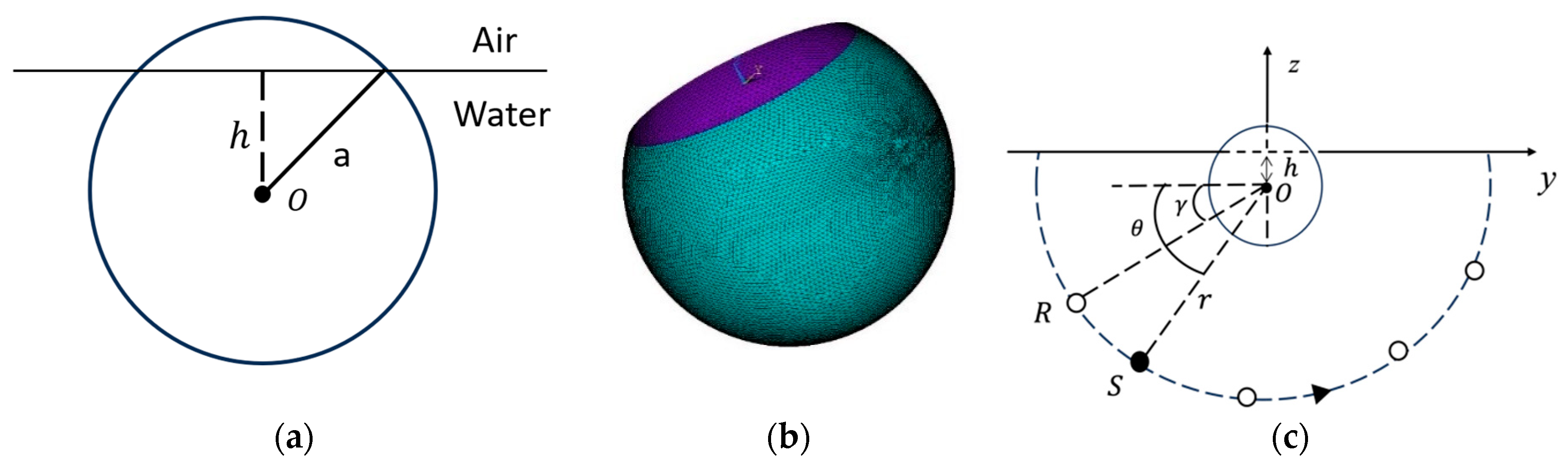
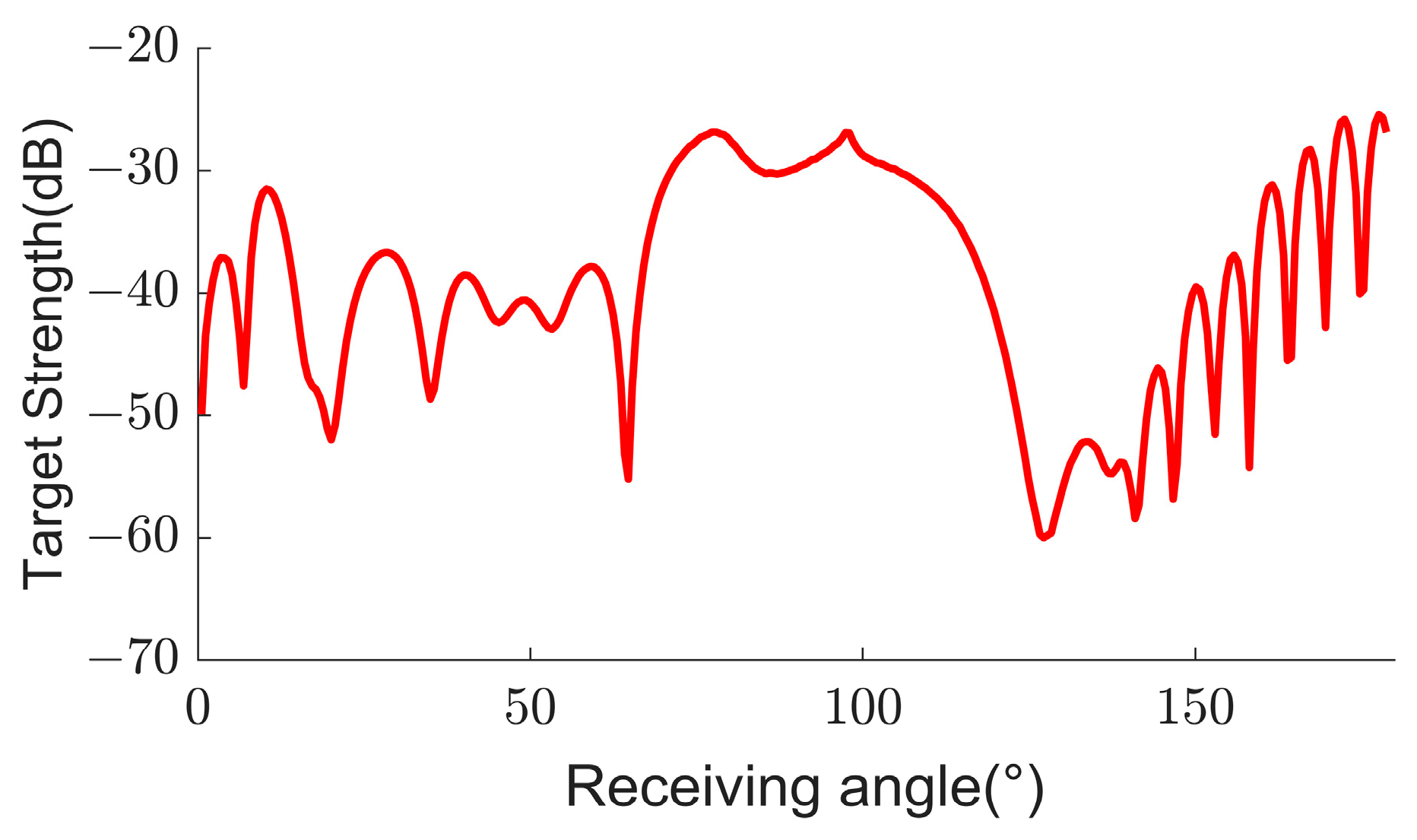
2.2. Simulation of the Signal Ice Ball Model

We conduct numerical experiments to simulate the acoustic scattering field of an ice ball floating on water. The experimental layout is depicted in Figure 3. Figure 3a depicts a schematic vertical cross-section of an ice ball floating in still water, where $a$ denotes the ball radius, and $h$ denotes the vertical distance from center point $O$ to the water surface. Applying the Archimedes principle of a floating ice ball on water, $F={\rho }_{ice}g{V}_{ice}=\rho g(V_{ice}-V_{cap})$, for a given ball radius $a,h$ can be solved from the following derivation,

$$1-{\displaystyle \frac{{\rho }_{ice}}{\rho }}={\displaystyle \frac{V_{cap}}{V_{ice}}}={\displaystyle \frac{\pi {(a-h)}^2\left(a-\frac{a-h}{3}\right)}{\frac{4}{3}\pi a^3}}$$

(18)

where $V_{ice}$ indicates the ice volume, $V_{cap}$ denotes the partial volume of the ice ball that is above water, and ${\rho }_{ice}$ indicates the ice density.

The portion of the ball exposed above the water surface is excluded in the analysis since it does not affect the underwater acoustic scattering field. The underwater portion of the ice ball surface is divided by the element segmentation through the Delaunay triangulation method, as illustrated in Figure 3b. Figure 3c shows a schematic of the single ice ball model employing a bistatic configuration with a transmitting transducer and a receiving transducer. In this layout, the horizontal direction y is parallel to the water surface. The source $S$ and receiver $R$ are located on an arc with a radius $r$, and centered at $O$. The grazing angle $\theta$ is defined as the angle between the original sound wave direction and the horizontal direction. While the receiving angle γ is the angle between $R-O$ and the horizontal direction, varying between 0° and 180°.

To compare with laboratory experimental data addressed in Section 2.3 later, we choose the model parameters unless otherwise specified, including $a=5$ cm, $\rho =1000 \mathrm{kg}/{\mathrm{m}}^3$, ${\rho }_{ice}=915 \mathrm{kg}/{\mathrm{m}}^3, \mathrm{and} c=1500 \mathrm{m}/\mathrm{s}$. We note that salinity levels in both ice and water are critical in affecting the underwater sound speed and refraction, and the participation of the submerged ice surface in the underwater acoustic scattering. In our model, the salinity effects are implicitly introduced by the choice of model parameters, such as the densities of ice and water, sound speed, and absorption coefficient. Model parameters are selected to satisfy specific salinity levels in the calculation of target or scattering intensities within our model.

Applying the incident wave on the ball surface and under far-field conditions, we can calculate the target strength against receiving angle $\gamma$ by Equation (17). For $\theta =$ 45°, Figure 4 shows that the target strength of the ice ball fluctuates greatly when the receiving angle is less than 60° or greater than 120°. The fluctuations can be attributed to the occurrence of the additional wave paths caused by multiple scattering between the ice ball and the water surface. The latter results in lager differences in the wave phase of the echo signal for each path. Because of the independences of the path-related bright regions and the signals received at each angle, the target strength curve does not show symmetry. In the bright spot model, the presence of the water surface increases the inherent bright spot from the free-field case, thus resulting in a complex echo structure of the floating ice ball.

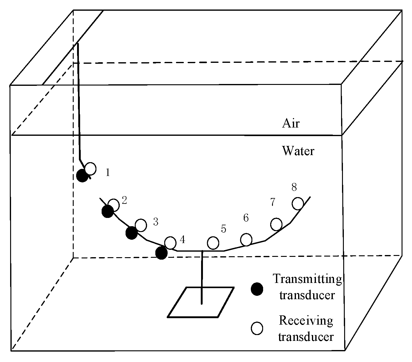
2.3. Water Tank Experiment

To validate the theoretical simulation mentioned earlier, we conducted a laboratory experiment in a water tank to measure the target strength in a single ice ball model. The laboratory experiment layout is depicted in Figure 5. Here, an ice ball is centrally positioned on the water surface in a water tank. The dimensions of the water tank were 1.4 m in length, 1.2 m in width, and 1.2 m in height, and the water depth was 1.1 m. Sound-absorbing wedges were attached to both sides of the tank walls to further reduce the wall scattering noises. The transmission signal is a CW pulse signal at a frequency of 90 kHz, with a single continuous wave duration of 0.2 ms and a signal interval of 1 s. This configuration of long pulse interval and short duration aids in the distinction between the object backscattering signal and the wall scattering noise. Transmitting the transducer sound source level and the receiving transducer sensitivity were tested in prior, and the results are detailed in the Appendix A.

The transducers were mounted in a pre-made curved steel frame mounted at the tank bottom. Some of these transducers are observed as black boxes in Figure 5. Given the potential of deviations from the intended design angles during the fabrication of the steel frame and the installation of the transducers onto the frame, we measured the angle of each transducer relative to a reference plane after they were placed in the slots. A high-precision digital inclinometer was used for this purpose, aligned with the vertical axis, and multiple measurements were taken to determine the final installation angles of the transducers. We use a transmitting transducer with grazing angle θ = 30° and an array of five receiving transducers with receiving angles γ = 30°, 45°, 60°, 73°, and 90°, respectively. The angles of the receiving transducer and the distances between the receiving transducers and the ice ball center are given in

Table 1. Receiving angles of transducers and distances between the receiving transducers and the ice ball centers.

Transducers	1	2	3	4	5
Angle (°)	30	45	60	73	90
Distance (m)	0.65	0.75	0.80	0.81	0.80

. The experimental duration was short enough to ignore the ice melting in the cool water. Therefore, we did not measure the ice ball’s mass or volume post-experiment to estimate the melting impact. To minimize experimental error, we replicated each experiment four times by measuring the scattering acoustic signals. Steady-state values from the measured signal waveforms are selected to obtain the averages.

The target strength can be written as

$$TS=20\log \left|{\displaystyle \frac{r{r}_{i}g{e}_{oc}/M}{p_{ref}g·{10}^{\frac{SPL}{20}}}}\right|$$

(19)

where $r$ is the distance between the receiving transducer and the ice ball surface, and $r_i$ is the distance from the sound source point to the ice ball surface, $g$ is gravity acceleration, $p_i$ indicates the valid sound pressure value at the receiver, and $p_{ref}=1 \mathsf{\mu }\mathrm{P}\mathrm{a}$ is the reference source pressure in water, then the acoustic pressure level is calculated through $SPL=20\log \left({\displaystyle \frac{p_i}{p_{ref}}}\right)$. Additionally, $M={\displaystyle \frac{e_{oc}}{p_0}}$ is the acoustic pressure sensitivity of the receiver where $e_{oc}$ indicates the open-circuit voltage output by the transducer.

By substituting the measured data into Equation (19), we calculate the target strengths at the five selected receiving angles. The measured target strengths are depicted as blue dots in Figure 6 along with the theoretical simulation (red curve), as a function of the receiving angle. To quantify the agreement between the experimental and simulation results, the average of absolute errors across the receiving angles is calculated as 2.91 dB. The bias is considered acceptable within the scope of our study for validating the single ice ball model discussed in Section 2.

Note that errors in our study can arise from both theoretical modeling and experimental procedures. Theoretically, we model the ice ball as an elastic sphere with resistance, simulating wave scattering within a semi-infinite domain. This simplification may introduce discrepancies between the modeling and the measurements, which contributes to the errors. Experimentally, errors can arise from several sources. For instant, the positioning of the ice ball and the transducers in the laboratory setup may deviate from ideal conditions. Additionally, the ice ball may not be perfectly spherical with the homogenous reflection feature due to mold constraints and laboratory environmental conditions with even slight melting potentially affecting the acoustic wave scattering. Experimental errors could also come from factors including the precise positioning the transducer, the distance between the transducer and the target, variations in the transducer’s sound source level, and the instruments’ sensitivity.

3. Acoustic Scattering under Ice Water Interface with Multiple Ice Balls

In this section, we further consider scenarios that feature multiple ice balls with both uniform and non-uniform distributions. We investigate the corresponding underwater acoustic scattering fields through numerical simulations and conduct relevant water tank experiments for comparison.

3.1. Theory of Multiple Ice Balls Model

The acoustic scattering field of multiple ice balls floating on water is more complex than the single ice ball case mentioned above. To simplify the problem, we represent the acoustic scattering intensity at a specific location by superposing the acoustic scattering fields generated by each ice ball within the domain. However, we neglect the effects of multiple scattering and occlusion among the spheres. Additionally, Bragg scattering [26] is not considered due to the micro-scale roughness on the ball surface falling outside the scope of this study. Generally, assuming there are N ice balls floating in water, the scattering potential function at a given location is formulated as:

$${\varphi }_{Sall}={\sum }_{n=1}^N{\varphi }_{S_n}+{\varphi }_{water}$$

(20)

where ${\varphi }_{S_n}$ indicates the scattering potential function of the n-th ice ball and ${\varphi }_{water}$ indicates the scattering potential function from the water surface.

In the bistatic transducer configuration case, the scattering potential function can be simplified as

$${\varphi }_s=\underset{M\to \mathrm{\infty }}{lim}{\sum }_{m=1}^M({\phi }_{s1}+{\phi }_{s2}+{\phi }_{s3}+{\phi }_{s4}{)}_m$$

(21)

where

$$({\phi }_{s1}{)}_m=-{\displaystyle \frac{jk}{4\pi }}{\displaystyle \frac{e^{jk(r_q+r_m)}}{r_q{r}_m}}V(\beta )\left[{\displaystyle \frac{jk{r}_q-1}{jk{r}_q}}\mathit{cos}{\theta }_1+{\displaystyle \frac{jk{r}_m-1}{jk{r}_m}}\mathit{cos}{\theta }_2\right]S_{m1}$$

(22)

$$({\phi }_{s2}{)}_m=-{\displaystyle \frac{jk}{4\pi }}{\displaystyle \frac{e^{jk\left(r_q+r_k\right)}}{r_q{r}_k}}{V}_b\left(\alpha \right)\left[V\left(\beta \right){\displaystyle \frac{\left(jk{r}_q-1\right)}{jk{r}_q}}\mathit{cos}{\theta }_1+V\left(\beta \right){\displaystyle \frac{\left(jk{r}_k-1\right)}{jk{r}_k}}\mathit{cos}{\theta }_2\right]S_{m2}$$

(23)

$$({\phi }_{s3}{)}_m=-{\displaystyle \frac{jk}{4\pi }}{\displaystyle \frac{e^{jk\left(r_z+r_m\right)}}{r_z{r}_m}}{V}_b\left(\alpha \right)\left[V\left(\beta \right){\displaystyle \frac{\left(jk{r}_z-1\right)}{jk{r}_z}}\mathit{cos}{\theta }_1+V\left(\beta \right){\displaystyle \frac{\left(jk{r}_m-1\right)}{jk{r}_m}}\mathit{cos}{\theta }_2\right]S_{m3}$$

(24)

$$({\phi }_{s4}{)}_m=-{\displaystyle \frac{jk}{4\pi }}{\displaystyle \frac{e^{jk\left(r_z+r_k\right)}}{r_z{r}_k}}{V}_b^2\left(\alpha \right)\left[V\left(\beta \right){\displaystyle \frac{\left(jk{r}_z-1\right)}{jk{r}_z}}\mathit{cos}{\theta }_1+V\left(\beta \right){\displaystyle \frac{\left(jk{r}_k-1\right)}{jk{r}_k}}\mathit{cos}{\theta }_2\right]S_{m4}.$$

(25)

Due to the different reflection characteristics among ice scattering and the multiple scattering interactions between ice and water, we utilize the scattering intensity as the metric, rather than target strength, for the acoustic scattering field beneath the ice–water interface. The scattering intensity $S_s$ is defined as the ratio of the sound intensity scattered by a unit volume or area to the incident wave sound intensity at a reference distance of 1 m, formulated as

$$S_s=10{\log \left|{\displaystyle \frac{I_s}{I_i}}\right|}_{r=1m}.$$

(26)

For the incident wave with potential function ${\varphi }_i={\displaystyle \frac{e^{jk{r}_{10}}}{r_{10}}}$, the scattering intensity under the ice–water interface is further given as

$$S_s=10\log {\displaystyle \frac{{\left|\frac{r_{20}{\varphi }_{sall}}{{\varphi }_i}\right|}^2}{A}}$$

(27)

where $r_{10}$ is the distance between the sound source and the center of the interface, $r_{20}$ is the distance between the receiving point and the center of the interface, and $A$ represents the horizontal area of the ice–water interface.

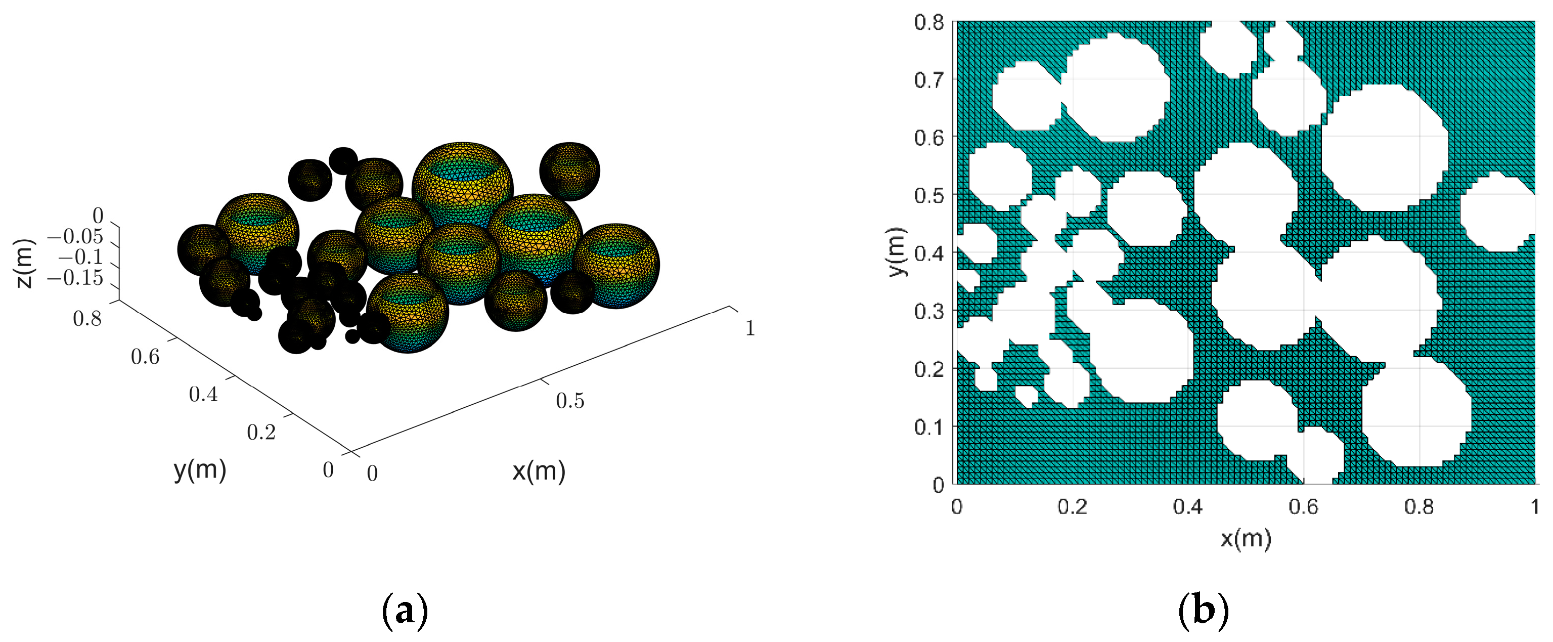
3.2. Simulation of Multiple Ice Balls Floating in Water

We first focus on modeling the acoustic scattering field associated with an ice–water interface consisting of equally sized ice balls distributed uniformly. Specifically, the ice balls were placed at equidistant grid nodes on a two-dimensional water surface, forming a regular grid pattern. As with the single ice ball model, each modeled sphere is divided into multiple smaller surface elements using the Delaunay triangulation method. By removing the segments of the balls above the water, the resulting three-dimensional surface element division of the balls’ surface submerged in water is shown in Figure 7a. Moreover, Figure 7b gives a top view of the triangular elements of the water surface (x-y plane) after removal of the ice balls.

Using these surface meshes with surfel division, the scattering intensities of the ice spheres and the water surface are calculated individually using Equation (27). The calculations are performed at the ‘receiver’ located along an arc, which keeps a consistent distance between the sound source S and the mean coordinates of the ice balls. These scattering intensities of the two are then superimposed to obtain the overall scattering intensity of the ice–water interface.

Figure 8 illustrates the total scattering intensity from the ice–water interface (red dash) and its components from the ice balls (blue dot–dash) and the water surfaces (green solid) as a function of the receiving angle γ. In these simulations, we set the grazing angle θ to 45° as in the single ice ball model. It is observed that when γ is small, the scattering intensity of the ice–water interface is in good agreement with that of the ice ball component. However, the scattering intensity of the ice ball rapidly deviates from the other components as γ exceeds 120°, in which the reflection component of the water surface plays a crucial role for larger γ. This discrepancy is mostly pronounced for γ within the approximate range of 120° to 160°. The peak scattering intensity occurs at γ = 135°, where the intensity from the water surface component becomes dominant and much larger than that of the ice balls.

We further investigate the scattering behavior of non-uniformly distributed ice balls in water, where the ice–water interface consists of randomly sized ice balls floating in the still water. In the simulation setup, we designate a horizontal domain of $1 \mathrm{m}\times 0.8 \mathrm{m}$ for the ice–water interface, with an ice concentration varying from 4/10 to 5/10. Figure 9a illustrates an example of the ice balls’ surface element division, where the ice balls of varying diameters are distributed in the water, satisfying the specified ice concentration constraints. The scattering intensity for a given ice–water interface is determined using the method applied for the uniformly distributed ice balls. To obtain a robust statistical scattering intensity for this random scenario, we simulate 100 repetitions to calculate an average scattering intensity for the random ice–water interface cases. Figure 9b presents the resulting average scattering intensity, which also includes the individual contributions from reflections off the free surface and reflections from the ice balls surfaces.

For the non-uniformly distributed ice–water interface, Figure 10 illustrates the relationship between the receiving angle γ and the scattering intensity. When γ is far away from the mirror reflection angle, the scattering intensity is mainly influenced by the surface scattering of the ice balls, compared with the fluctuations of the water surface reflection. However, as γ approaches the mirror reflection angle, the influence of the water surface reflection becomes significant. Notably, at a grazing angle of 30°, corresponding to a mirror reflection angle of 150°, the reflection from the water surface reaches the maximum, resulting in a peak scattering intensity of the ice–water interface.

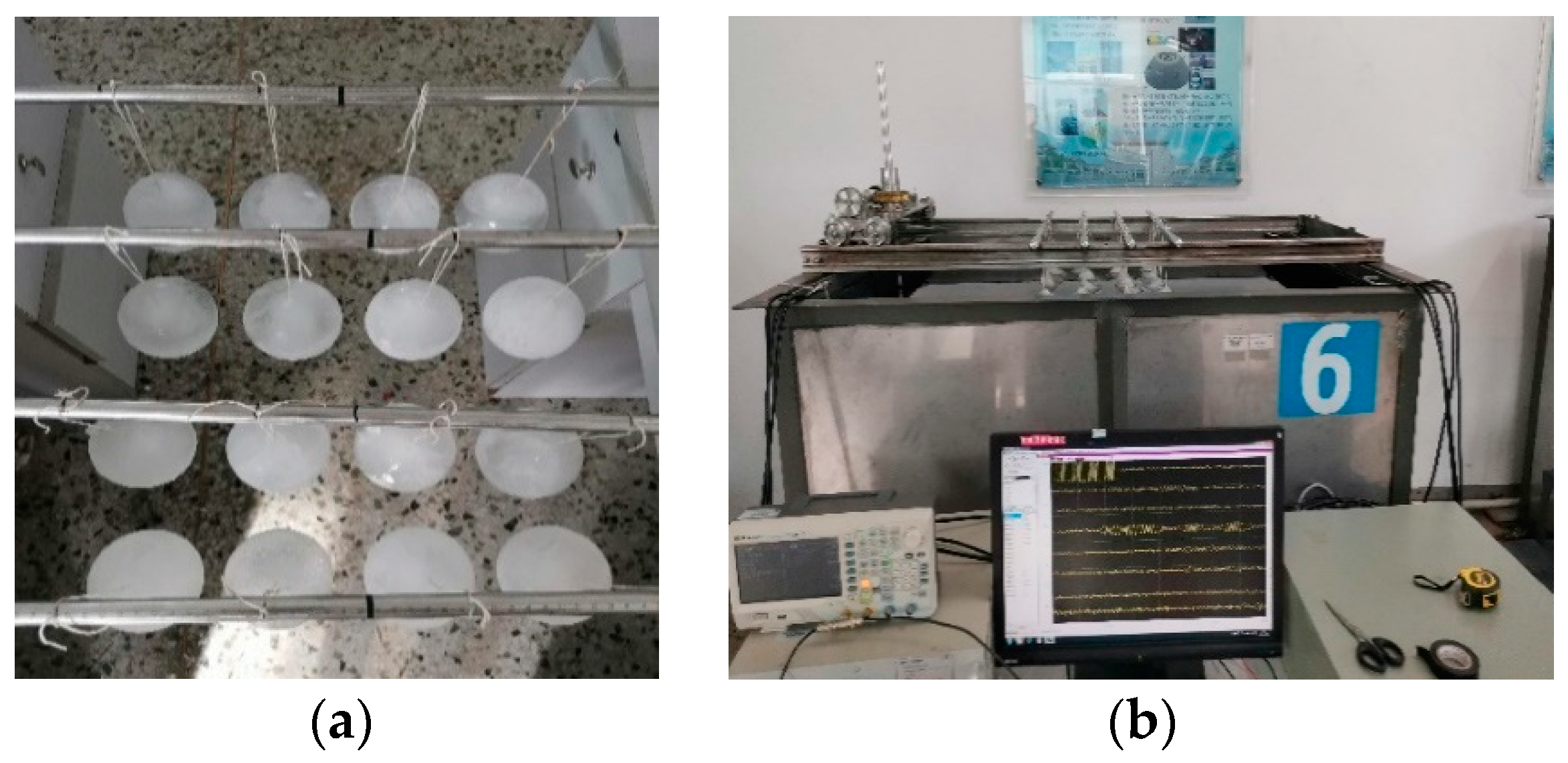
3.3. Experiments of Multiple Ice Balls Floating in a Water Tank

We carried out a series of water tank experiments to measure the scattering intensity, to validate our model for the multiple ice balls situations. The experimental setup is depicted in Figure 11. The same water tank and transmission signal were utilized as in the single ice ball experiment. Transmitting transducers (solid circles) and receiving transducers (hollow circles) were mounted on a transducer base array frame with the scattering azimuth of 0°. The grazing angles θ corresponding to the transmitting transducers were selected as 30°, 42°, 56°, and 70°. Meanwhile, the receiving transducers were positioned at angles of 30°, 45°, 60°, 73°, 90°, 107°, 121°, and 135°. Both sound source levels of the transmitting transducer and the sensitivity of the receiving transducer were measured prior to the experiments. These measurements are detailed in the Appendix A.

A total of 16 equal-sized ice balls were prepared in one experiment. These ice balls were tied with strings and suspended beneath iron rods, as shown Figure 12a. This setup allowed the ice balls to float freely in the water while maintaining the uniform distribution. Figure 12b depicts the overall layout of the experiment, where the acoustic signals are collected in a water tank by the receiving transducer and transmitted to a computer for further analysis.

The scattering intensity of the ice–water interface can be obtained as

$$S_S=10\log \left|{\displaystyle \frac{e_s^2{r}_1^2{r}_2^2}{P_{inc0}^2{M}^2{A}_M}}\right|$$

(28)

where the sound pressure value at the transmitting transducer $P_{inc0}$ is obtained before the experiment. Its value is converted from the known sound source level of the transmitting transducer and the sensitivity of the receiving transducer M. Therefore, in the actual measurement, it is necessary to record several parameters, including the distance between the receiving transducer and the center of the horizontal domain in the water tank, denoted as $r_1$, and the distance between the transmitting transducer and the center of the horizontal domain $r_2$, the echo voltage of the ice–water interface $e_s$, and the area of ice–water interface within the beam range of the transducers $A_M$.

Figure 13 shows the scattering intensities obtained between the experimental and the simulated results for grazing angles: 30°, 42°, 56°, and 70°. The simulated curve exhibits high fluctuations across the chosen receiving angles. The smaller grazing angle correlates with the larger receiving angles where maximum scattering intensity is observed. Despite this variation, the experimental data are generally within the range of the simulated scattering intensity, indicating good agreement between the simulated and observed results. The absolute errors between the simulation and experimental data over the receiver positions are given in

Table 2. Absolute errors averaged over receiving locations for uniformly distributed ice balls.

$\mathrm{Grazing} \mathrm{angle} \theta$ (°)	30	42	56	70
Error (dB)	3.1	2.13	3.68	2.92

, with the absolute errors being generally less than 4 dB for the examined grazing angles. In addition to the discussion in Section 2.3, it is noteworthy that the potential bias of placing the transducers could be important due to the sensitivity of calculated scattering intensity regarding to the receiving angle. Considering the comprehensive errors, the validity of our methodology can be proved. This agreement further confirms the robustness of our model in capturing the scattering intensities.

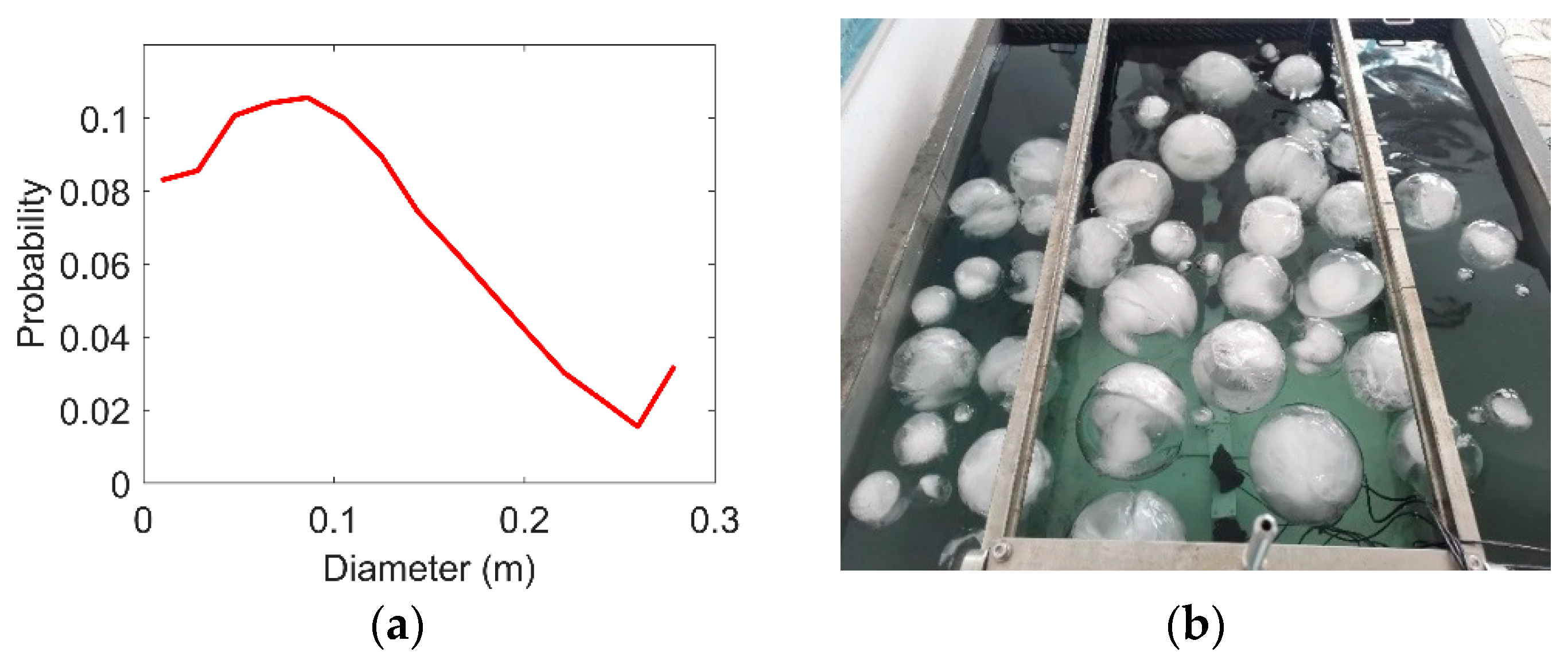
3.4. Experiments of Randomized Ice Balls Floating in a Water Tank

We further present water tank measurements of the scattering fields for the non-uniformly distributed ice–water interface. To compare the statistical properties of the laboratory experiments and the simulations, we estimated the diameter distribution of the ice balls using the numerical approach previously described for the generation of the non-uniformly distributed ice–water interface. Specifically, we carried out 100 generations of randomly distributed ice balls within a $1.4 \mathrm{m}\times 1.2 \mathrm{m}$ domain, matching the horizontal extent of the water tank. The density distribution of the ice balls is set to 45/m². The resulting probability for the ice ball diameter generation is presented in Figure 14a. This probability curve guided the selection of ice balls for the experiments. However, due to the limitation in mold sizes available for preparing ice balls, it is difficult to prepare ice ball diameters exactly according to the probability curve. Therefore, the actual selection of ice ball sizes in the experiments was an approximation derived from this probability curve. An example of the non-uniform distribution of ice balls floating in the water tank is illustrated in Figure 14b.

We conducted a series of 12 experiments with different randomly distributed ice–water interfaces within the water tank, maintaining a consistent concentration of ice balls throughout.

Table 3. Sizes and number of ice balls used in the water tank experiments.

Diameter (cm)	3	5	6	8	9	10	12
Amount	5	5	6	6	7	6	6
Diameter (cm)	14	16	18	20	22	24	26
Amount	5	4	3	3	3	2	4

summarizes the specific diameters of the ice balls and their respective counts for these experiments. For each experiment, we measured the acoustic signals at different grazing and receiving angles, as depicted in Figure 11. Steady-states of the acquisition waveforms are selected to calculate the average voltage, which is then substituted into Equation (28) to compute the scattering intensity of the ice–water interface for the non-uniform ice balls.

Figure 15 presents the scattering intensities obtained from experimental measurements (blue dots) and simulations (red curves). Furthermore, to enhance the visualization of the overall trends in the simulated data, a 20-degree moving average window was applied to the red curve, marked as the smoothed black curves. The two sets of data are generally in good agreement. As the receiving angle approaches the mirror reflection angle of the incident wave, there is an increasing trend of the scattering intensity. Conversely, the scattering intensity decreases as the receiving angle diverges from the mirror reflection angle. Notably, when the receiving angle diverges from the mirror reflection angle, the scattering intensity contributed by the ice surfaces becomes predominant, leading to better agreement between the simulated and experimental results. However, when the receiving angle is closer to the mirror reflection angle, the mirror reflection component from the sound wave passing through the water surface becomes larger, leading to larger discrepancies between the observations and simulations. The respective absolute errors averaged over all the receiving angles are given in

Table 4. Absolute errors averaged over receiving locations for non-uniformly distributed ice balls in water.

Grazing angle $\theta$ (°)	30	42	56	70
Error (dB)	2.64	1.83	3.64	3.73

for each case. In general, the mean absolute error over these grazing angles is within 3 dB.

4. Discussion and Conclusions

This study presents a groundwork for future development of acoustic scattering methodologies considering the influence of real ice in the marginal ice zones of polar oceans. Simplifying the complexity of a real ice environment, we conceptualized an individual ice floe (similar to brash ice, with a thickness comparable to its floe size) as a sphere with acoustic resistance. Given the intricacies of multiple scattering, our focus was on the analysis of the principal scattering waves to evaluate the underwater acoustic scattering field. Applying numerical simulations, we segmented the ice–water interface into finely divided elements through the plate element method. We then analyzed the acoustic scattering path for each discrete element and culminated in comprehensive evaluations, such as the target intensity and scattering strength. The key conclusions drawn from this study are as follows:

• The underwater acoustic field in the presence of ice floes on the water surface is discussed. The multiple scatterings between the ice balls and the free surface lead to a complex echo structure. We analyze the resulting acoustic field by selecting the primary contributors, such as the direct wave in the free field, the echo due to the virtual source, and two scattering waves between the ice ball and water surfaces in a single ice ball model.
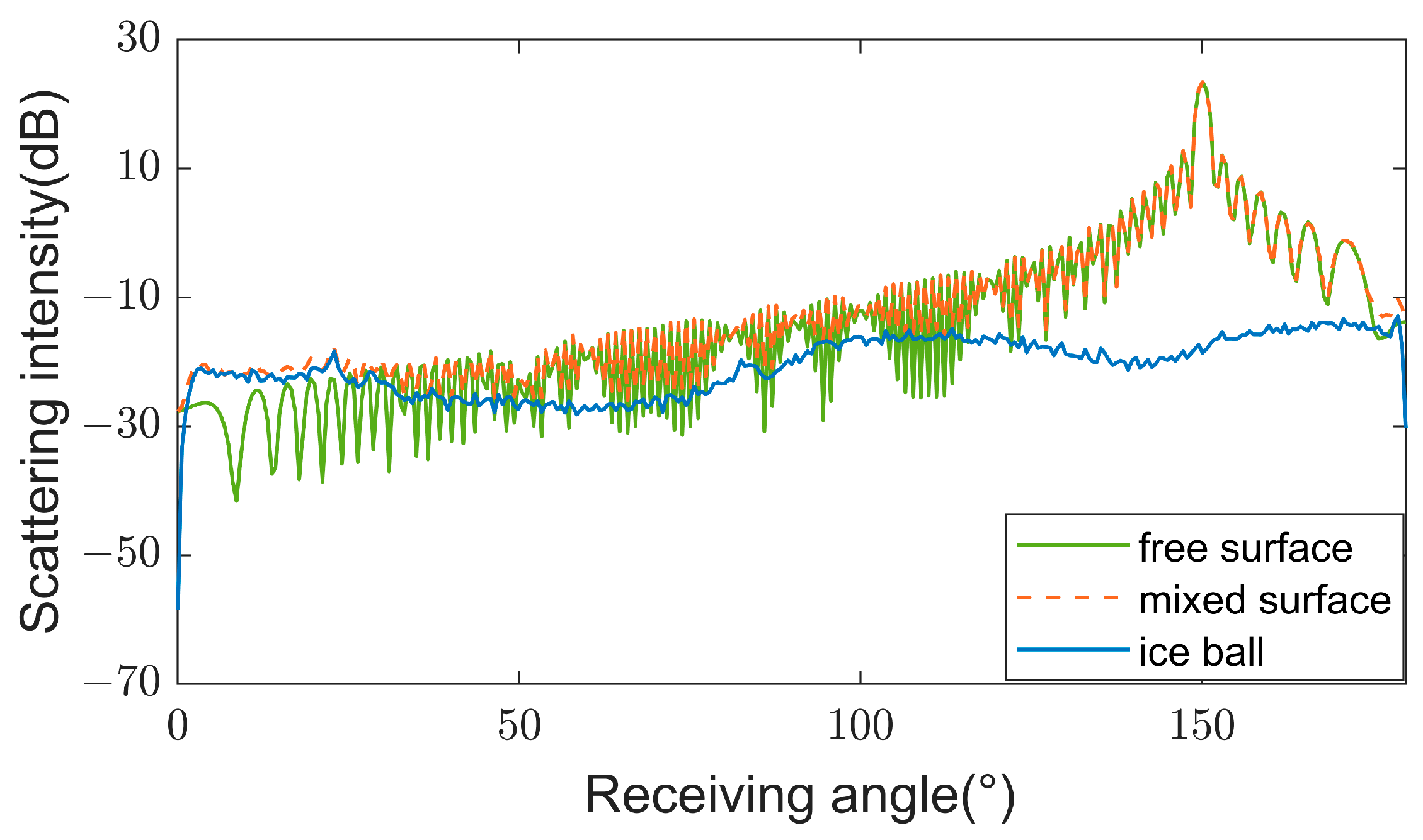
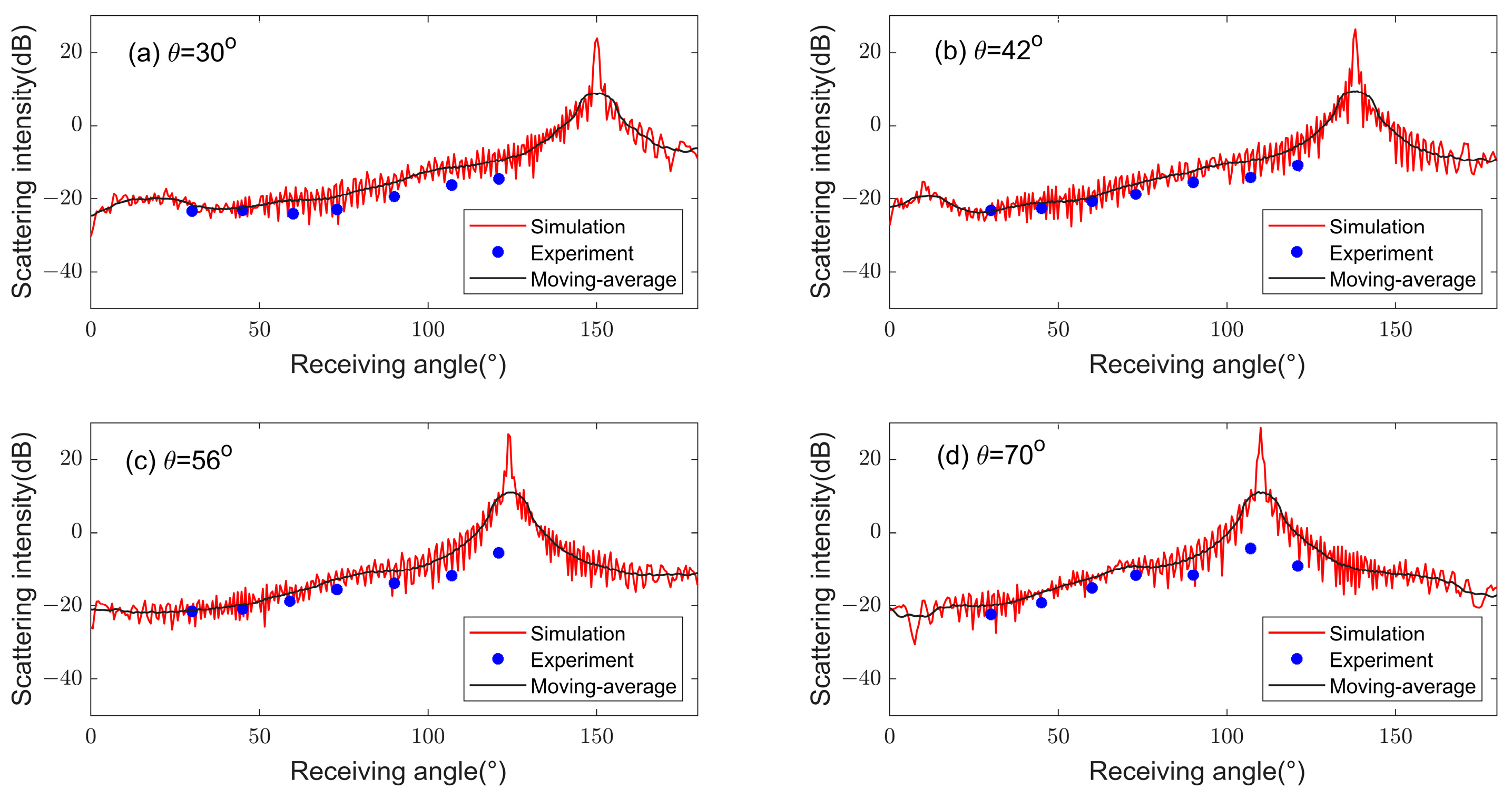
• Based on the analysis of the scattering acoustic field, we establish a single ice ball model to calculate the target strength. The model is then extended to two cases with multiple ice balls in water: one model is established for uniformly distributed ice balls, and another model is established for non-uniformly distributed ice balls. The scattering intensity for the corresponding ice–water interfaces is calculated, including reflections from the surfaces of submerged ice balls and the free water surface. The results indicate that when the receiving angle is close to the incident acoustic wave’s mirror reflection angle, the scattering intensity positively correlates with the reflection component of the water surface.
• The scattering intensity measured in a water tank is used to validate the theoretical models. For the uniformly distributed ice–water interface, the average error over the receiving angles is found to be within 3 dB, thereby verifying the validity of the model while considering the analysis error. For the non-uniformly distributed ice–water interface, the experimental and simulation results show consistent trends, and the average error is also within 3 dB. The best agreement between the measured and simulated results occurs when the receiving angle is far from the mirror reflection angle, whereas larger errors are observed when the receiving angle is near the mirror reflection angle.
• The overall good agreement between the experimental and theoretical results supports the effectiveness of our methods for analyzing complex acoustic scattering in the presence of ice–water interfaces. We acknowledge the bias from non-uniform distribution and sizes of the ice balls from both modeling and experimental perspectives. From a modeling perspective, we simplified an ice ball as a sphere with resistance and simulated wave scattering in a semi-infinite domain. From an experimental perspective, ice balls cannot be precisely located in the water tank and may move or melt during the experiment. The ice balls randomly generated by the simulation are approximated by the limited number of molds used to freeze ice balls. Moreover, the number of experiments might be insufficient to obtain unbiased statistical variables.

References

1. Zhu, G.; Yin, J.; Chen, W.; Hu, S.; Zhou, H.; Guo, L. Modeling and characteristics of acoustic channel under typical arctic ice. Acoust. Acta Sin. 2017, 42, 152–158. [Google Scholar]
2. Hutt, D. An overview of Arctic Ocean acoustics. In AIP Conference Proceedings; American Institute of Physics: College Park, MD, USA, 2012; Volume 1495. [Google Scholar]
3. Morozov, A.K.; Altshuler, T.W.; Jones, T.C.P.; Freitag, L.E.; Koski, P.A.; Singh, S. Underwater acoustic technologies for long-range navigation and communications in the Arctic. In Proceedings of the International Conference on Underwater Acoustic Measurements, Kos, Greece, 20–24 June 2011; Papadakis, J.S., Bjorno, L., Eds.; Technologies & Results. 2011. [Google Scholar]
4. Alexander, P.; Duncan, A.; Bose, N.; Smith, D. Modelling Acoustic Transmission Loss Due to Sea Ice Cover. Acoust. Aust. 2013, 41, 79–87. [Google Scholar]
5. Freitag, L.; Koski, P.; Singh, S.; Maksym, T.; Singh, H. Acoustic communications under shallow shore-fast Arctic ice. In Proceedings of the OCEANS 2017-Anchorage, Anchorage, AK, USA, 18–21 September 2017; pp. 1–5. [Google Scholar]
6. Mccammon, D.F.; Mcdaniel, S.T. The influence of the physical properties of ice on reflectivity. Acoust. Soc. Am. J. 1985, 77, 499–507. [Google Scholar] [CrossRef]
7. Liu, S.; Li, Z. Reflection and scattering characteristics of sea ice on sound waves. Acta Phys. Sin. 2017, 66, 206–213. [Google Scholar]
8. Lucieer, V.; Nau, A.W.; Forrest, A.L.; Hawes, I. Fine-Scale Sea Ice Structure Characterized Using Underwater Acoustic Methods. Remote Sens. 2016, 8, 821. [Google Scholar] [CrossRef]
9. Jiang, M.; Chen, X.; Xu, L.; Clausi, D.A. IceGCN: An Interactive Sea Ice Classification Pipeline for SAR Imagery Based on Graph Convolutional Network. Remote Sens. 2024, 16, 2301. [Google Scholar] [CrossRef]
10. Garrison, G.; Early, E. Acoustic backscattering from uniform Arctic Sea ice. In Proceedings of the IEEE International Conference on Engineering in the Ocean Environment, Halifax, NS, Canada, 21–23 August 1974. [Google Scholar]
11. Ito, M.; Ohshima, K.I.; Fukamachi, Y.; Mizuta, G.; Kusumoto, Y.; Nishioka, J. Observations of frazil ice formation and upward sediment transport in the Sea of Okhotsk: A possible mechanism of iron supply to sea ice. J. Geophys. Res. Ocean. 2017, 122, 788–802. [Google Scholar] [CrossRef]
12. Huang, H.; Gaunaurd, G. Exact analysis of the acoustic scattering by an arbitrarily insonified spherical body near a flat boundary. J. Acoust. Soc. Am. 1994, 95, 2946. [Google Scholar] [CrossRef]
13. Huang, H.; Gaunaurd, G. Scattering of a plane acoustic wave by a spherical elastic shell near a free surface. Int. J. Solids Struct. 1997, 34, 591–602. [Google Scholar] [CrossRef]
14. Gaunaurd, G.; Huang, H. Sound scattering by bubble clouds near the sea surface. J. Acoust. Soc. Am. 2000, 107, 95–102. [Google Scholar] [CrossRef] [PubMed]
15. Richardson, M.E.; Briggs, K.B.; Williams, K.L.; Jackson, D.R.; Naval Research Lab Stennis Space Center Ms Marine Geosciences Div. Scattering of High-Frequency Acoustic Energy from Discrete Scatterers on the Seafloor: Glass Spheres and Shells. Proc.-Inst. Acoust. 2001, 23, 369–374. [Google Scholar]
16. Kungl, A.F.; Schumayer, D.; Frazer, E.K.; Langhorne, P.J.; Leonard, G.H. An oblate spheroidal model for multi-frequency acoustic back-scattering of frazil ice. Cold Reg. Sci. Technol. 2020, 177, 103122. [Google Scholar] [CrossRef]
17. Simon, B.; Isakson, M.; Ballard, M. Modeling acoustic wave propagation and reverberation in an ice covered environment using finite element analysis. In Proceedings of the Meetings on Acoustics 175ASA, Minneapolis, MN, USA, 7–11 May 2018; Acoustical Society of America: Melville, NY, USA, 2018; Volume 33, p. 070002. [Google Scholar]
18. Chen, W.; Hu, S.; Wang, Y.; Yin, J.; Korochensev, V.I.; Zhang, Y. Study on acoustic reflection characteristics of layered sea ice based on boundary condition method. Waves Random Complex Media 2021, 31, 2177–2196. [Google Scholar] [CrossRef]
19. Chen, W.; Sun, H.; Wang, W. Study on calculation method of target strength in waveguide. In Proceedings of the 2016 IEEE/OES China Ocean Acoustics (COA), Harbin, China, 9–11 January 2016; pp. 1–4. [Google Scholar]
20. Peng, X. The effects of the sail on acoustic scattering characteristics of the underwater structure. In Proceedings of the INTER-NOISE and NOISE-CON Congress and Conference, New Orleans, LA, USA, 29 June–1 July 2020; Institute of Noise Control Engineering: Wakefield, MA, USA, 2020; Volume 261, pp. 4382–4388. [Google Scholar]
21. Abawi, A.T. Kirchhoff scattering from underwater targets modeled as an assembly of triangular facets. J. Acoust. Soc. Am. 2009, 125, 2608. [Google Scholar] [CrossRef]
22. Lavia, E.F.; Gonzalez, J.D.; Blanc, S. Modeling high-frequency backscattering from a mesh of curved surfaces using Kirchhoff Approximation. J. Theor. Comput. Acoust. 2019, 27, 1850057. [Google Scholar] [CrossRef]
23. Seybert, A.F.; Wu, T.W. Modified Helmholtz integral equation for bodies sitting on an infinite plane. J. Acoust. Soc. Am. 1989, 85, 19–23. [Google Scholar] [CrossRef]
24. Tang, W. Calculation of acoustic scattering from object near an interface using physical acoustic method. Acta Acust.-Peking- 1999, 24, 1–5. [Google Scholar]
25. Williams, K.L.; Marston, P.L. Synthesis of backscattering from an elastic sphere using the Sommerfeld–Watson transformation and giving a Fabry–Perot analysis of resonances. J. Acoust. Soc. Am. 1986, 79, 1702–1708. [Google Scholar] [CrossRef]
26. Gurcan, M.; Creasey, D.J.; Gazey, B.K. Development of a sonar to measure the size of sea-bed material. In Proceedings of the Acoustics and the Sea-Bed Conference, Bath, UK, 6–8 April 1983; pp. 357–365. [Google Scholar]
Figure 1. Schematic diagram of principal scattering paths selected in a single ice ball model for monostatic transducer setup.
Remotesensing 16 03113 g001
Figure 2. Schematic diagram of principal scattering paths selected in a single ice ball model for the biostatic transducer setup.
Remotesensing 16 03113 g002
Figure 3. Numerical modeling of a signal ice ball floating in water; (a) vertical section view of the ice ball in water; (b) panel division diagram of an ice ball surface submerged in water; and (c) layout of the bistatic transducer setup.
Remotesensing 16 03113 g003
Figure 4. Simulated target strength over receiving angle γ for a signal ice ball model.
Remotesensing 16 03113 g004
Figure 5. Experimental layout of a single ice ball model in a water tank.
Remotesensing 16 03113 g005
Figure 6. Comparison of measured and theoretical target strength against receiving angle γ .
Remotesensing 16 03113 g006
Figure 7. Surfel division for a uniformly distributed ice water interface. (a) Surface elements of ice balls submerged in water. (b) Surface elements grid of the free surface.
Remotesensing 16 03113 g007
Figure 8. Scattering intensities of a uniformly distributed ice–water interface versus receiving angle γ .
Remotesensing 16 03113 g008
Figure 9. Surfel division for a non-uniformly distributed ice–water interface. (a) Surface elements of ice balls submerged in water. (b) Surface elements grid of the free surface.
Remotesensing 16 03113 g009
Figure 10. Scattering intensities averaged over 100 non-uniformly distributed ice–water interfaces against receiving angle γ .
Remotesensing 16 03113 g010
Figure 11. Schematic diagram of transmitting and receiving transducers in a water tank.
Remotesensing 16 03113 g011
Figure 12. Experiment setup for a uniformly distributed ice balls case, (a) prepared ice ball tied under iron rods, and (b) the experimental layout.
Remotesensing 16 03113 g012
Figure 13. Scattering intensities against receiving angle γ for uniformly distributed ice balls in water.
Remotesensing 16 03113 g013
Figure 14. (a) Probability of ice ball diameters for the case of non-uniformly distributed ice balls, and (b) an example of non-uniformly distributed ice balls in water.
Remotesensing 16 03113 g014
Figure 15. Scattering intensities against the receiving angle γ for non-uniformly distributed ice balls in water.
Remotesensing 16 03113 g015