MFO-Fusion: A Multi-Frame Residual-Based Factor Graph Optimization for GNSS/INS/LiDAR Fusion in Challenging GNSS Environments

Abstract

In various practical applications, such as autonomous vehicle and unmanned aerial vehicle navigation, Global Navigation Satellite Systems (GNSSs) are commonly used for positioning. However, traditional GNSS positioning methods are often affected by disturbances due to external observational conditions. For instance, in areas with dense buildings, tree cover, or tunnels, GNSS signals may be obstructed, resulting in positioning failures or decreased accuracy. Therefore, improving the accuracy and stability of GNSS positioning in these complex environments is a critical concern. In this paper, we propose a novel multi-sensor fusion framework based on multi-frame residual optimization for GNSS/INS/LiDAR to address the challenges posed by complex satellite environments. Our system employs a novel residual detection and optimization method for continuous-time GNSS within keyframes. Specifically, we use rough pose measurements from LiDAR to extract keyframes for the global system. Within these keyframes, the multi-frame residuals of GNSS and IMU are estimated using the Median Absolute Deviation (MAD) and subsequently employed for the degradation detection and sliding window optimization of the GNSS. Building on this, we employ a two-stage factor graph optimization strategy, significantly improving positioning accuracy, especially in environments with limited GNSS signals. To validate the effectiveness of our approach, we assess the system’s performance on the publicly available UrbanLoco dataset and conduct experiments in real-world environments. The results demonstrate that our system can achieve continuous decimeter-level positioning accuracy in these complex environments, outperforming other related frameworks.

1. Introduction

Global Navigation Satellite System (GNSS) technology has become the backbone of numerous navigation applications, owing to its exceptional ability to deliver precise spatio-temporal data [1]. However, traditional GNSS navigation is vulnerable in challenging GNSS environments and can be significantly impaired due to noise-induced jitter, compromising the overall navigation accuracy [2,3]. As precision in positioning is crucial across various applications, this flaw seriously undermines the utility of traditional GNSS navigation systems. Similarly, conventional LiDAR-inertial odometry (LIO) [4], despite its wide usage owing to its real-time 3D mapping capabilities, comes with its own set of drawbacks. One major problem is the deviation of navigation paths. Even with LiDAR’s high pointing accuracy, there can be a notable drift over time in trajectories estimated by LIO. Such deviation becomes more noticeable during extended journeys, resulting in a significant offset in navigation paths.

Advanced navigation and mapping applications have benefited greatly from the unique precision and reliability achieved through the amalgamation of GNSS, INS, and LiDAR technologies [5]. In multi-sensor fusion for positioning, integrating different ranging sources plays a crucial role in enhancing anti-spoofing capabilities. By checking the consistency between outputs from various sensors, such as GNSS, IMU, and LiDAR, the system can effectively detect and counter GNSS spoofing attacks. Relevant studies highlight the importance of improving the security and reliability of navigation systems [6,7,8]. However, in challenging terrains like urban canyons, forests, and tunnels, where GNSS signals might be obstructed or degraded, the performance of these systems can seriously decline. To counter these challenges, recent developments in the sensor fusion field have demonstrated promising potential in augmenting the accuracy and robustness of navigation and mapping systems. Scholars have extensively investigated multi-sensor integrated navigation systems, categorizing the methodologies into loosely-coupled and tightly-coupled paradigms [9,10,11]. Loosely-coupled approaches are known for their flexibility and efficiency; however, they often suffer from suboptimal performance due to inevitable information loss, especially in environments with severe sensor degradation [12,13,14,15]. In these systems, each sensor’s data are processed independently, and the results are fused at a higher level, which can lead to significant information gaps. On the other hand, tightly-coupled methodologies are designed to maximize the exploitation of multi-sensor information, significantly enhancing navigation and positioning precision [16,17,18,19,20,21]. Tightly-coupled systems integrate data at a lower level, directly combining raw sensor inputs, which allows for a more comprehensive and robust use of available information. This approach not only improves accuracy but also maintains system performance and stability even when individual sensors experience failures or performance degradation. While tightly-coupled systems are more complex to implement, their superior precision and reliability make them ideal for high-stakes applications requiring consistent and accurate navigation data.

Among these advancements, factor graph optimization (FGO) [22] has emerged as an effective means of compiling measurements from multiple sensors to estimate a system’s status. Nonetheless, traditional sensor fusion techniques often fail to deliver in difficult environments, where individual sensor measurement quality varies significantly, leading to sub-par system performance. The complex nature of fusion algorithms, along with the high computational cost for processing data from multiple sensors, might impede the system’s real-time performance. Moreover, current fusion techniques may not optimally harness the continuous-time information provided by sensors like GNSS, INS, and LiDAR, which could potentially fine-tune the accuracy of navigation and mapping systems.

To address these challenges, we propose a novel MFO-Fusion framework that leverages the multi-frame residual of GNSS/INS/LiDAR measurements and employs sophisticated factor graph optimization algorithms to achieve a robust and accurate fusion of sensor data. By incorporating continuous frame information and leveraging advanced optimization techniques, MFO-Fusion aims to overcome the limitations of traditional sensor fusion approaches and provide a more reliable navigation and mapping solution in challenging environments. Our design provides the following contributions:

(1)

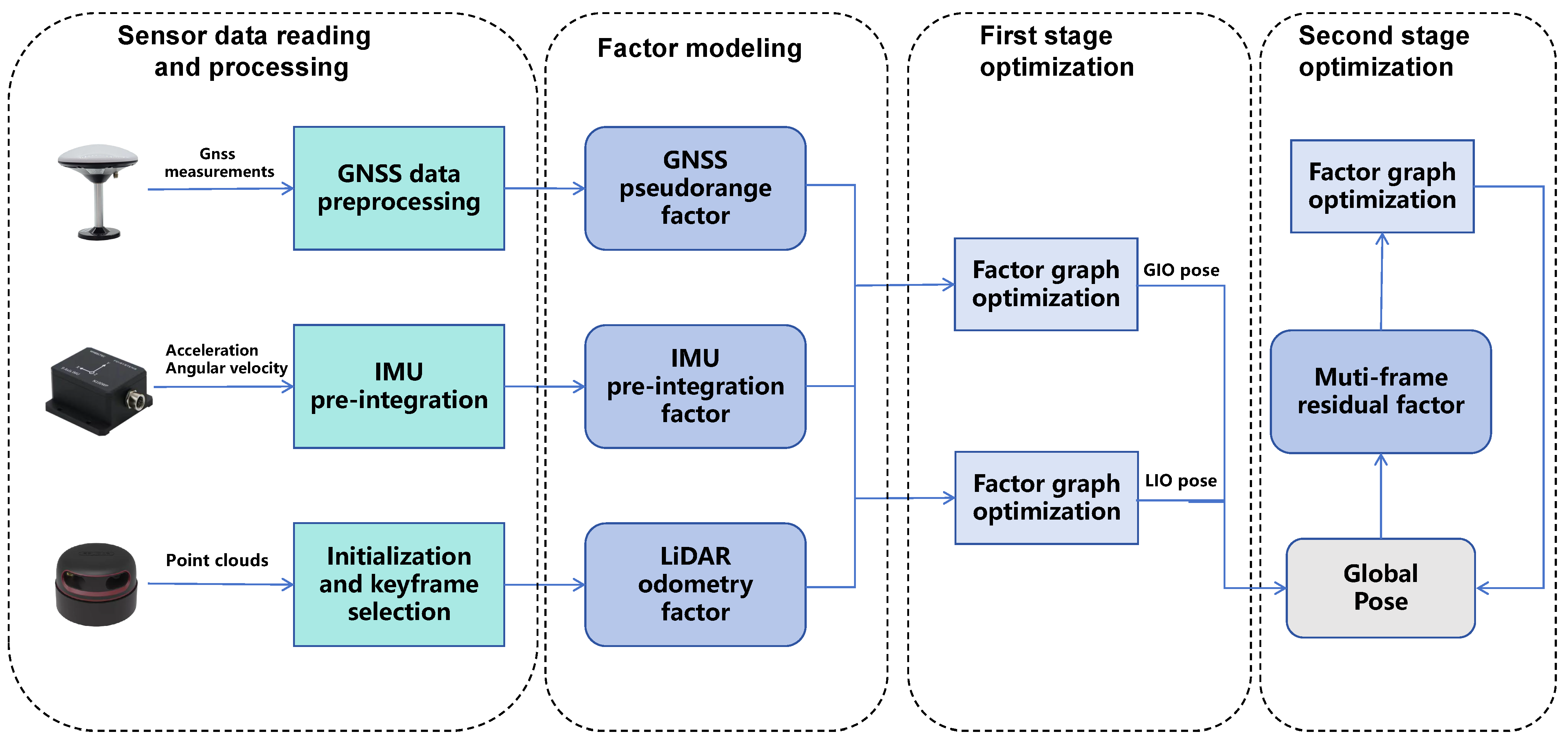
A factor graph-optimized odometry framework based on GNSS, IMU, and LiDAR is proposed, which tightly integrates GNSS pseudorange measurement, IMU attitude measurement, and LiDAR point cloud measurement for precise and stable positioning in complex scenes;

(2)

A fusion strategy based on two-stage optimization was proposed, and a multi-frame residual factor was introduced for outlier detection and the calibration of positioning errors, achieving robust and globally consistent state estimation;

(3)

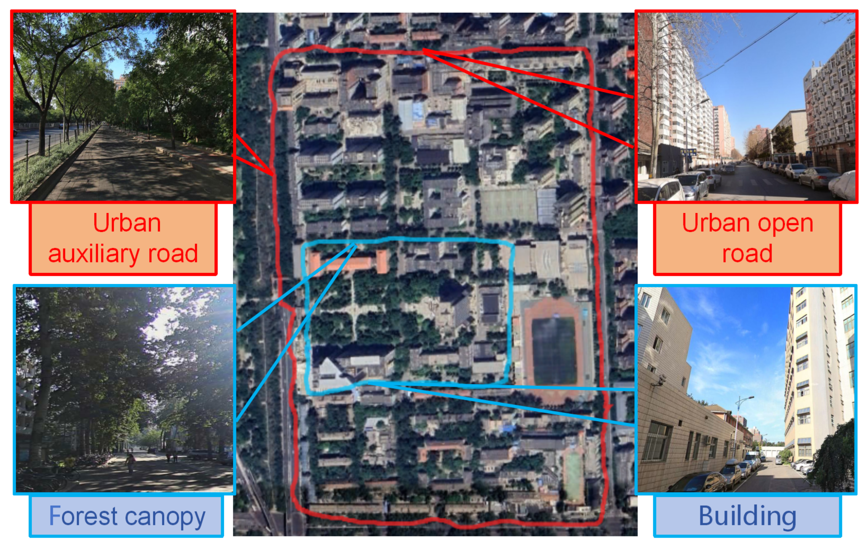
The proposed method has been extensively experimentally validated in both public urban challenge scenarios and complex on-site scenarios, demonstrating its effectiveness.

The rest of this paper is organized as follows. In Section 2, we provide an overview of related work in the fields of sensor fusion and factor graph optimization. In Section 3, we describe the MFO-Fusion framework in detail, including the multi-frame residual of GNSS/INS/LiDAR measurements and the factor graph optimization algorithms. In Section 4, we present the experimental results of MFO-Fusion in challenging environments and compare its performance with existing fusion techniques. Finally, in Section 6, we conclude the paper and discuss potential future research directions in the field of sensor fusion for challenging GNSS environments.

2. Related Work

Recent advancements in GNSS/INS and LiDAR-based sensor fusion have significantly improved navigation and positioning accuracy in challenging environments. Dual-sensor integration, such as GNSS/INS and LiDAR/INS, has been a focus of research. Meanwhile, multi-sensor systems that combine GNSS, INS, and LiDAR are emerging. We introduce the research progress of dual- and multi-sensor GNSS/INS/LiDAR in the following content.

2.1. Dual-Sensor Integrated Localization

The integration of dual sensors for attitude positioning and navigation has been a hot topic among researchers. For GNSS/INS integration, a robot-centered iterative error-state Kalman filter (ESKF) has been devised to achieve precise and efficient pose estimation in a tightly-coupled manner [16]. Additionally, a robust time-differenced carrier phase (TDCP) closed-loop method based on factor graphs has been proposed to enhance the integrated performance of tightly-coupled GNSS/IMU systems [17]. This method involves cycle slip detection to eliminate its influence during the closed-loop formation, leveraging Doppler shift for detection and selecting corresponding carrier phase measurements to construct TDCP loop closures for improved positioning performance. The performance of tightly-coupled GNSS/IMU integrations has also been analyzed using single-station and network GNSS stations, along with post-processing kinematics methods, with a specific focus on forward Kalman filtering and smoothing algorithms [18]. Furthermore, a novel GNSS positioning enhancement method based on 3D LiDAR has been introduced [19], which utilizes a sliding window map for real-time detection of non-visible range satellites and implements effective deviation correction through reflection point correction and measurement uncertainty reconstruction. A refined strong tracking unscented Kalman filter (RSTUKF) is developed to enhance robustness against kinematic model error [23]. An online constrained-optimization method has also been proposed to simultaneously estimate attitude and other related parameters, benefiting from self-initialization without the need for prior attitude or sensor measurement noise information [24]. Additionally, a method based on the recurrent neural network (RNN) has been introduced, utilizing the calculation principle of INS and the memory function of RNN to estimate INS errors, providing a continuous, reliable, and high-precision navigation solution even in GNSS-denied environments [25].

For LiDAR/INS integration, an integrated INS/LiDAR SLAM navigation system has been proposed to improve positioning results in challenging GNSS environments by utilizing an extended Kalman filter (EKF) [26]. A LiDAR-assisted inertial navigation system, combining commercial IMU and LiDAR, optimizes the search range of SLAM, using the original IMU output to establish stable long-term navigation in GNSS-restricted environments. This system applies a global scanning matching algorithm based on non-feature extraction grid maps, which offers higher accuracy and stability with lower computational complexity compared to other radar scanning matching schemes [27]. A tightly-coupled LiDAR–IMU SLAM algorithm has been proposed for the accurate and robust estimation of position, attitude, velocity, and deviation in under-featured off-road environments [20]. To mitigate accumulated errors and address environmental degradation, a closed-loop detection method that incorporates inertial measurement unit (IMU) and LiDAR information has been presented [21]. Initially, an odometer calculation method based on an iterative extended Kalman filter (IEKF) is introduced, integrating key LiDAR features and IMU data to improve FAST-LIO [28] initial attitude estimation accuracy. Subsequently, in the closed-loop detection process, a novel global descriptor for scanning context is developed, considering both geometry and intensity information. This descriptor is constructed from the distortion feature points of the front-end IMU, enhancing closed-loop detection accuracy compared to the original point cloud descriptor. Finally, GTSAM [22] is employed for global optimization, integrating GPS constraints to mitigate trajectory drift and achieve globally consistent trajectories and maps.

2.2. Multi-Sensor Integrated Localization

A GNSS–IMU–LiDAR constrained Kalman filtering approach [29] is proposed for mobile platform attitude estimation. This method employs scalable factor graph optimization for multi-sensor data fusion to construct high-precision odometers. Original GNSS observations are introduced to enhance LiDAR–IMU calibration, eliminating the need for predefined targets [30]. To achieve stable and accurate navigation in urban canyon environments, a LiDAR-aided continuous GNSS-RTK positioning method with GNSS smart selection functionality is proposed [31]. LIO progressively generates locally accurate motion estimates and point cloud maps. Then, based on LiDAR environmental description, urbanization level, and GNSS signal quality assessment, available GNSS-RTK in light urban areas is detected. Finally, integrated with LIO optimization results, continuous accurate positioning is achieved in highly urban areas, with low-drift LIO local estimates and global GNSS correction, resulting in significant performance improvement compared to non-GNSS integration. A tightly-coupled data fusion system of GNSS, INS, and visual odometry [32] is designed, employing error-state extended Kalman filtering for multi-sensor integration, tightly-coupled pseudorange, and carrier phase measurements via double-difference RTK model, and further integrating stereo visual odometry with multi-constraint Kalman filtering to enhance positioning performance. To improve RTK performance in challenging GNSS environments, ref. [33] fuses the raw data via extended Kalman filter (EKF), improving positioning accuracy and refining direction and velocity estimates.

To address the degradation in localization and calibration due to asynchronous and outlier measurements, an enhanced adaptive factor graph is proposed for GNSS/IMU/odometer integrated synchronous localization and calibration (SLAC). This new framework constructs variable nodes based on odometer measurements and uses IMU preintegration to handle asynchronous GNSS positions, with noise parameters estimated via an Expectation-Maximization (EM) algorithm [34,35]. A tightly-coupled fusion method with fixed lag smoothing improves robustness through enhanced LiDAR registration [36]. Further optimizations include a Two-Phase Sensor Fusion (TPSF), combining GNSS, LiDAR, and IMU data [37]; a mapping method that integrates LiDAR, IMU, and GNSS data with vertical drift mitigation [38]; a robust fusion odometer system with GNSS–IMU for coarse state estimation and LiDAR–IMU for refined mapping [39]; and the GLIO estimator for globally consistent attitude estimation using a two-stage optimization scheme [40].

3. Materials and Methods

3.1. System Overview

We first define the coordinate system frames and related notation used in the paper. We set the latitude, longitude, and altitude (LLA) coordinate system, where the GNSS receiver is located as $\mathbf{L}$, and the Earth Center Earth Fixed Frame (ECEF) coordinate system, where the GNSS satellite is located as $\mathbf{E}$. The East–North–Up (ENU) coordinate system $\mathbf{N}$ serves as the coordinate system for the the vehicle body. Moreover, we set the coordinate system of the LiDAR as $\mathbf{C}$ and the IMU as $\mathbf{B}$. The vehicle body’s state variable x is commonly represented according to the conventional approach,

$$\begin{array}{cc}\hfill x& ={\left[p,v,q,b_{\mathrm{g}},b_{\mathrm{a}},g\right]}^{\top }\hfill \end{array}$$

(1)

where p, v, and q represent the position, velocity, and rotation of the vehicle body at a specific moment. Specifically, p and v are three-dimensional vectors, while $q\in SO\left(3\right)$ represents a rotation matrix in the form of a Lie group. $b_{\mathrm{g}}$ and $b_{\mathrm{a}}$, respectively, represent the bias of the gyroscope and accelerometer within the IMU. The parameter g represents the acceleration of gravity, as shown in Figure 1.

The system collects data from GNSS receivers, IMUs, and LiDAR sensors and estimates the vehicle body’s posture status and trajectory changes using initial data observations. The problem of pose estimation can be defined as the Maximum Posteriori Problem (MAP), which is modeled and solved using factor graphs. Under the assumption of a Gaussian noise model, our problem can be reformulated as a least squares problem and subsequently solved. Firstly, we designated three types of sensors as GPS-inertial odometry and LiDAR-inertial odometry. The sensors inside the odometry utilize a tightly-coupled factor graph optimization strategy. After optimizing the initial loose coupling between the two odometries, we proceed to use the multi-frame residual factor and conduct a secondary optimization. In the following sections, we introduce our odometry generation process, the generation method of multi-frame residual factor, and the secondary optimization strategy.

3.2. GPS-Inertial Odometry

We use the factor graph optimization method to initially establish the GPS-inertial odometry subsystem. The specific processing logic of the odometry is as follows. Firstly, the algorithm for external static IMU initialization is used to determine the bias and gravity direction. Subsequently, the GNSS signal is utilized to obtain the initial position. When the IMU data arrive, we use the pre-integration method to accumulate information about the IMU’s pose changes. After receiving GNSS data, we formulate a graph optimization problem using the previous and current GNSS information. We incorporate a pre-integration factor and GNSS pseudorange factor as constraints. Notably, we initialize the optimization process with the predicted values of IMU pre-integration.

3.2.1. GNSS Pseudorange Factor

The pseudorange of the i-th satellite in a GNSS receiver can be modeled in the following form:

$$\begin{array}{c}\hfill {\rho }_{\mathrm{GPS}}^i=r^i+c\delta t_r-c\delta t_s+c{I}^i+c{T}^i+{\tilde{\epsilon }}_{\rho }^i\end{array}$$

(2)

where ${\rho }_{\mathrm{GPS}}^i$ is the measured pseudorange of the i-th satellite, $r^i$ is the actual distance between the signal receiver and the satellite transmission antenna, $\delta t_r$ is the receiver clock deviation, c is the speed of light, $\delta t_s$ is the satellite clock deviation, $I^i$ is the ionospheric delay, $T^i$ is the tropospheric delay, and ${\tilde{\epsilon }}_{\rho }^i$ is the noise and multipath error. Satellite clock errors are typically corrected using the clock correction parameters transmitted within the satellite navigation message. Ionospheric errors can be corrected using dual-frequency GNSS signals, which allow for the estimation and removal of ionospheric delay effects by examining the differences in signal delay between the two frequencies [41]. As a result, it is possible to simplify the equation to

$$\begin{array}{c}\hfill {\rho }_{\mathrm{GPS}}^i=r_{\mathrm{GPS}}^i+c\delta t_r+{\tilde{\epsilon }}_{\rho }^i\end{array}$$

(3)

The actual distance $r_{\mathrm{GPS}}^i$ from the satellite receiver to the i-th satellite is

$$\begin{array}{c}\hfill r_{\mathrm{GPS}}^i=\sqrt{{\left(x-x^i\right)}^2+{\left(y-y^i\right)}^2+{\left(z-z^i\right)}^2}=∥\mathit{p}-{\mathit{p}}_{\mathrm{S}}^i∥\end{array}$$

(4)

where x, y, and z represent the 3D position of the GNSS receiver in the ECEF coordinate system. Define the pseudo-distance received by the IMU as

$$\begin{array}{c}\hfill {\rho }_{\mathrm{INS}}^i=\sqrt{{\left(x_{\mathrm{INS}}-x^i\right)}^2+{\left(y_{\mathrm{INS}}-y^i\right)}^2+{\left(z_{\mathrm{INS}}-z^i\right)}^2}=∥{\mathit{p}}_{\mathrm{INS}}-{\mathit{p}}_{\mathrm{S}}^i∥\end{array}$$

(5)

Thus, the pseudorange error between the GPS and INS of the i-th satellite is

$$\begin{array}{c}\hfill {\rho }_{\mathrm{GPS}}^i-{\rho }_{\mathrm{INS}}^i=∥\mathit{p}-{\mathit{p}}_{\mathrm{S}}^i∥-∥{\mathit{p}}_{\mathrm{INS}}-{\mathit{p}}_{\mathrm{S}}^i∥+c\delta t_r+{\tilde{\epsilon }}_{\rho }^i\end{array}$$

(6)

Due to the disparate coordinate systems of GNSS satellites and INS, it is necessary to execute suitable coordinate system transformations to ensure consistency in the calculation of residuals. Given that the IMU resides in the vehicle coordinate system B, the GNSS receiver operates in the LLA coordinate system, and the GPS satellite operates in the ECEF coordinate system. Given the pose in the ENU coordinate system, the rotation of the pose from the ENU coordinate system to the ECEF coordinate system is

$$\begin{array}{c}\hfill {\mathbf{R}}_n^e=\left[\begin{array}{ccc}-sin\lambda & -sin\varphi cos\lambda & cos\varphi cos\lambda \\ cos\lambda & -sin\varphi sin\lambda & cos\varphi sin\lambda \\ 0& cos\varphi & sin\varphi \end{array}\right]\end{array}$$

(7)

where $\varphi$ and $\lambda$ represent the latitude and longitude of the reference point in the geographic coordinate system. Using this rotation matrix, given that the rotation matrix ${\mathbf{R}}_l^n$, ${\mathbf{R}}_b^n$ between the satellite receiver and the vehicle body coordinate system concerning the ENU coordinate system is known, we can derive the expression for the residual as

$$\begin{array}{c}\hfill r_{\mathcal{P}}\left({\tilde{\mathbf{z}}}_{L,B,S}^i,\mathcal{X}\right)=∥{\mathbf{R}}_l^n{\mathbf{R}}_n^e{\mathit{p}}_{\mathrm{L}}^i-{\mathit{p}}_{\mathrm{S}}^i∥-∥{\mathbf{R}}_b^n{\mathbf{R}}_n^e{\mathit{p}}_{\mathrm{B}}^i-{\mathit{p}}_{\mathrm{S}}^i∥+c\delta t_r+{\tilde{\epsilon }}_{\rho }^i\end{array}$$

(8)

3.2.2. IMU Pre-Integration Factor

To ensure efficient integration of high-frequency IMU data and improve the accuracy and stability of multi-sensor fusion systems, we construct pre-integrated residual factors using the pre-integration method. This method accumulates accelerometer and gyroscope data from the IMU over longer time intervals, reducing computational load and smoothing high-frequency noise. This approach ensures more reliable data for fusion, accurately reflects the system’s nonlinear dynamics, and enhances the precision in complex motion environments.

A conventional IMU can measure the acceleration and angular velocity of object motion, but its observed values are affected by noise, bias, and gravity. Set the measured values to $\tilde{\mathit{\omega }}$, $\tilde{\mathit{a}}$; then, observations at time t can be modeled as follows:

$$\begin{array}{c}\hfill \begin{array}{cc}\hfill \tilde{\mathit{\omega }}\left(t\right)& =\mathit{\omega }\left(t\right)+{\mathit{b}}_{\mathrm{g}}\left(t\right)+{\mathit{\eta }}_{\mathrm{g}}\left(t\right)\hfill \\ \hfill \tilde{\mathit{a}}\left(t\right)& ={\mathit{R}}^{\top }(\mathit{a}\left(t\right)-\mathit{g})+{\mathit{b}}_{\mathrm{a}}\left(t\right)+{\mathit{\eta }}_{\mathrm{a}}\left(t\right)\hfill \end{array}\end{array}$$

(9)

where ${\mathit{b}}_{\mathrm{g}}$ and ${\mathit{b}}_{\mathrm{a}}$ are the zero deviation of the gyroscope and accelerometer, and ${\mathit{\eta }}_{\mathrm{g}}$, ${\mathit{\eta }}_{\mathrm{a}}$ are the measured Gaussian noise. The kinematic equations of the Inertial Measurement Unit (IMU) allow us to deduce the mathematical correlation between the measured variables and the state variables:

$$\begin{array}{c}\hfill \begin{array}{cc}\hfill \mathit{R}(t+\Delta t)& =\mathit{R}\left(t\right)Exp\left(\left(\tilde{\omega }-{\mathit{b}}_{\mathrm{g}}\left(t\right)-{\mathit{\eta }}_{\mathrm{gd}}\left(t\right)\right)\Delta t\right)\hfill \\ \hfill \mathit{v}(t+\Delta t)& =\mathit{v}\left(t\right)+\mathit{g}\Delta t+\mathit{R}\left(t\right)\left(\tilde{\mathit{a}}-{\mathit{b}}_{\mathrm{a}}\left(t\right)-{\mathit{\eta }}_{\mathrm{ad}}\left(t\right)\right)\Delta t\hfill \\ \hfill \mathit{p}(t+\Delta t)& =\mathit{p}\left(t\right)+\mathit{v}\left(t\right)\Delta t+{\displaystyle \frac{1}{2}}\mathit{g}\Delta t^2+{\displaystyle \frac{1}{2}}\mathit{R}\left(t\right)\left(\tilde{\mathit{a}}-{\mathit{b}}_{\mathrm{a}}\left(t\right)-{\mathit{\eta }}_{\mathrm{ad}}\left(t\right)\right)\Delta t^2\hfill \end{array}\end{array}$$

(10)

It is worth noting that we use the form of Lie groups to derive pre-integration, where $\mathit{R}\in SO\left(3\right)$ is the rotation of the object, $\mathit{v}$ is the velocity, and $\mathit{p}$ is the position. ${\mathit{\eta }}_{\mathrm{gd}}$, ${\mathit{\eta }}_{\mathrm{ad}}$ is the discretized random walk noise [42].

$$\begin{array}{c}\hfill \begin{array}{c}Cov\left({\mathit{\eta }}_{\mathrm{gd}}\left(t\right)\right)={\displaystyle \frac{1}{\Delta t}}Cov\left({\mathit{\eta }}_{\mathrm{g}}\left(t\right)\right)\hfill \\ Cov\left({\mathit{\eta }}_{\mathrm{ad}}\left(t\right)\right)={\displaystyle \frac{1}{\Delta t}}Cov\left({\mathit{\eta }}_{\mathrm{a}}\left(t\right)\right)\hfill \end{array}\end{array}$$

(11)

Given the discrete frames i and j, the cumulative variables of the IMU sensor are

$$\begin{array}{c}\hfill \begin{array}{cc}\hfill \Delta {\mathit{R}}_{ij}& \doteq {\mathit{R}}_i^{\top }{\mathit{R}}_j=\prod _{k=i}^{j-1}Exp\left(\left({\tilde{\omega }}_k-{\mathit{b}}_{\mathrm{g},k}-{\mathit{\eta }}_{\mathrm{gd},k}\right)\Delta t\right)\hfill \\ \hfill \Delta {\mathit{v}}_{ij}& \doteq {\mathit{R}}_i^{\top }\left({\mathit{v}}_j-{\mathit{v}}_i-\mathit{g}\Delta t_{ij}\right)=\sum _{k=i}^{j-1}\Delta {\mathit{R}}_{ik}\left({\tilde{\mathit{a}}}_k-{\mathit{b}}_{\mathrm{a},k}-{\mathit{\eta }}_{\mathrm{ad},k}\right)\Delta t\hfill \\ \hfill \Delta {\mathit{p}}_{ij}& \doteq {\mathit{R}}_i^{\top }\left({\mathit{p}}_j-{\mathit{p}}_i-{\mathit{v}}_i\Delta t_{ij}-{\displaystyle \frac{1}{2}}\mathit{g}\Delta t_{ij}^2\right)\hfill \\ & =\sum _{k=i}^{j-1}\left[\Delta {\mathit{v}}_{ik}\Delta t+{\displaystyle \frac{1}{2}}\Delta {\mathit{R}}_{ik}\left({\tilde{\mathit{a}}}_k-{\mathit{b}}_{\mathrm{a},k}-{\mathit{\eta }}_{\mathrm{ad},k}\right)\Delta t^2\right]\hfill \end{array}\end{array}$$

(12)

where $\Delta t$ is the accumulated time. Separating the observation part and noise part of the above equation, we can obtain the IMU pre-integration observation model:

$$\begin{array}{c}\hfill \begin{array}{c}\hfill \Delta {\tilde{\mathit{R}}}_{ij}={\mathit{R}}_i^{\top }{\mathit{R}}_{j}Exp\left(\delta {\mathit{\varphi }}_{ij}\right)\\ \hfill \Delta {\tilde{\mathit{v}}}_{ij}={\mathit{R}}_i^{\top }\left({\mathit{v}}_j-{\mathit{v}}_i-\mathit{g}\Delta t_{ij}\right)+\delta {\mathit{v}}_{ij}\\ \hfill \Delta {\tilde{\mathit{p}}}_{ij}={\mathit{R}}_i^{\top }\left({\mathit{p}}_j-{\mathit{p}}_i-{\mathit{v}}_i\Delta t_{ij}-{\displaystyle \frac{1}{2}}\mathit{g}\Delta t_{ij}^2\right)+\delta {\mathit{p}}_{ij}\end{array}\end{array}$$

(13)

where $\delta \mathit{\varphi }$, $\delta \mathit{v}$, $\delta \mathit{p}$ are the errors between the observed and inferred actual values. Consequently, the residual corresponding to the observed values and the predicted values derived from IMU pre-integration can be modeled as

$$\begin{array}{c}\hfill \begin{array}{c}{\mathbf{r}}_{\mathcal{B}}\left({\tilde{\mathbf{z}}}_j^i,\mathcal{X}\right)=\left[\begin{array}{c}\delta {\mathit{\varphi }}_{ij}\\ \delta {\mathit{v}}_{ij}\\ \delta {\mathit{p}}_{ij}\\ \delta {\mathbf{b}}_a\\ \delta {\mathbf{b}}_g\end{array}\right]\\ =\left[\begin{array}{c}log\left(\Delta {\tilde{\mathit{R}}}_{ij}^{\top }\left({\mathit{R}}_i^{\top }{\mathit{R}}_j\right)\right)\\ {\mathit{R}}_i^{\top }\left({\mathit{v}}_j-{\mathit{v}}_i-\mathit{g}\Delta t_{ij}\right)-\Delta {\tilde{\mathit{v}}}_{ij}\\ {\mathit{R}}_i^{\top }\left({\mathit{p}}_j-{\mathit{p}}_i-{\mathit{v}}_i\Delta t_{ij}-{\displaystyle \frac{1}{2}}\mathit{g}\Delta t_{ij}^2\right)-\Delta {\tilde{\mathit{p}}}_{ij}\\ {\mathbf{b}}_{aj}-{\mathbf{b}}_{ai}\\ {\mathbf{b}}_{gj}-{\mathbf{b}}_{gi}\end{array}\right]\end{array}\end{array}$$

(14)

To sum up, the optimization architecture of the factor graph of GPS-inertial odometry in the first stage is shown as follows:

$$\begin{array}{c}\hfill {\mathcal{X}}_{GIO}^{*}=argmin\left\{\sum _{i,j\in \mathcal{B}}{∥{\mathbf{r}}_B\left({\tilde{\mathbf{Z}}}_j^i,{\mathcal{X}}_{GIO}\right)∥}_{{\mathsf{\Omega }}_B}^2+\sum _{i\in \mathcal{P}}{∥r_p\left({\tilde{\mathbf{Z}}}_{L,B,S}^i,{\mathcal{X}}_{GIO}\right)∥}_{{\mathsf{\Omega }}_P}^2\right\}\end{array}$$

(15)

3.3. LiDAR-Inertial Odometry

The LiDAR-inertial odometry processes raw data from LiDAR and IMU systems to estimate an initial pose. Initially, significant features are extracted from the point cloud data, delivered by the LiDAR mechanism. Subsequently, a residual factor for the radar is constructed from these features. Thereafter, we merge the pre-integration factor with the LiDAR factor, thereby formulating the optimization problem throughout for the odometry.

The initial attitude derived from the IMU is employed to assist in initializing the LiDAR. After eliminating the influence of motion distortion, we extract edge and plane features by calculating the curvature of the point cloud in the region. Points with smaller curvature values mean better local smoothness, divided into planar points. Correspondingly, edge points are composed of points with larger curvature. The edge and plane features extracted from LiDAR frames at time $t_k$ are represented as ${\mathcal{F}}_{t_k}^e$ and ${\mathcal{F}}_{t_k}^p$, respectively.

Using each LiDAR frame for feature extraction and residual calculation results in excessive computational complexity. In order to reduce computational complexity and meet the needs of subsequent factor additions, we adopt a keyframe extraction strategy. When the body posture changes beyond the threshold, we extract the keyframe ${\mathbb{F}}_{i+1}$, corresponding to the posture node $x_{i+1}$. Within a sliding window $\left\{{\mathbb{F}}_i,\dots ,{\mathbb{F}}_{i+n}\right\}$, we extract multiple sub keyframes and form a local voxel map:

$$\begin{array}{c}\hfill {\mathcal{M}}_i=\left\{{\mathcal{M}}_i^e,{\mathcal{M}}_i^p\right\}\\ \hfill \mathrm{where}:{\mathcal{M}}_i^e={}^{\prime }{\mathcal{F}}_i^e{\cup }^{\prime }{\mathcal{F}}_{i+1}^e\cup \dots {\cup }^{\prime }{\mathcal{F}}_{i+n}^e\\ \hfill {\mathcal{M}}_i^p={}^{\prime }{\mathcal{F}}_i^p{\cup }^{\prime }{\mathcal{F}}_{i+1}^p\cup \dots {\cup }^{\prime }{\mathcal{F}}_{i+n}^p\end{array}$$

(16)

In order to match the current new keyframe with the sub map, we need to match the edge and plane features of the keyframe with the map frame to establish geometric constraints. The coordinate transformation formula of feature points is as follows:

$$\begin{array}{c}\hfill {}^W\mathbf{P}_i={\mathbf{R}}_{b_{k+1}}^e\left({\mathbf{R}}_l^b·{}^{l_{k+1}}{\mathbf{P}}_i+{\mathbf{p}}_l^b\right)+{\mathbf{p}}_{b_{k+1}}^e-{\mathbf{P}}_{\mathbf{0}}\end{array}$$

(17)

Based on the transformed edge and plane features, we construct the point-to-line and point-to-face distance residuals:

$$\begin{array}{c}\hfill {\mathbf{r}}_{{\mathcal{L}}^e}\left({\widehat{\mathbf{z}}}_i^e,\mathcal{X}\right)={\displaystyle \frac{\left|\left({}^W\mathbf{p}_{i+1,k}^e-{}^W\mathbf{p}_{u,\mathcal{M}}^e\right)\times \left({}^W\mathbf{p}_{i+1,k}^e-{}^W\mathbf{p}_{v,\mathcal{M}}^e\right)\right|}{\left|{}^W\mathbf{p}_{u,\mathcal{M}}^e-{}^W\mathbf{p}_{v,\mathcal{M}}^e\right|}}\\ \hfill {\mathbf{r}}_{{\mathcal{L}}^p}\left({\widehat{\mathbf{z}}}_i^p,\mathcal{X}\right)={\displaystyle \frac{\left|\begin{array}{c}\left({}^W\mathbf{p}_{i+1,k}^p-{}^W\mathbf{p}_{u,\mathcal{M}}^p\right)\\ \left({}^W\mathbf{p}_{u,\mathcal{M}}^p-{}^W\mathbf{p}_{v,\mathcal{M}}^p\right)\times \left({}^W\mathbf{p}_{u,\mathcal{M}}^p-{}^W\mathbf{p}_{w,\mathcal{M}}^p\right)\end{array}\right|}{\mid \left({}^W\mathbf{p}_{u,\mathcal{M}}^p-{}^W\mathbf{p}_{v,\mathcal{M}}^p\right)\times \left({}^W\mathbf{p}_{u,\mathcal{M}}^p-{}^W\mathbf{p}_{w,\mathcal{M}}^p\right)\mid }}\end{array}$$

(18)

For the detailed derivation of the residual formula, refer to LIO-SAM [4]. Similar to the factor graph optimization of GPS-inertial odometry, the factor graph optimization modeling of LiDAR-inertial odometry is

$$\begin{array}{c}\hfill {\mathcal{X}}_{LIO}^{*}=argmin\left\{\sum _{i,j\in \mathcal{B}}{∥{\mathbf{r}}_B\left({\tilde{\mathbf{Z}}}_j^i,{\mathcal{X}}_{LIO}\right)∥}_{{\mathsf{\Omega }}_B}^2+\sum _{i\in {\mathcal{L}}^e}\rho \left({∥{\mathbf{r}}_{{\mathcal{L}}^e}\left({\widehat{\mathbf{z}}}_i^e,{\mathcal{X}}_{LIO}\right)∥}_{{\mathsf{\Omega }}_{{\mathcal{L}}^e}}^2\right)+\right.\\ \hfill \left.\sum _{i\in {\mathcal{L}}^p}\rho \left({∥{\mathbf{r}}_{{\mathcal{L}}^p}\left({\widehat{\mathbf{z}}}_i^p,{\mathcal{X}}_{LIO}\right)∥}_{{\mathsf{\Omega }}_{{\mathcal{L}}^p}}^2\right)\right\}\end{array}$$

(19)

3.4. Multi-Frame Residual Factor

As discussed above, the single-frame optimization of GNSS/INS is significantly limited in challenging GNSS environments, and the tight coupling between LiDAR and IMU is also affected by long-term drift. After obtaining the pose information of two odometries, we introduce a new multi-frame residual factor for continuous multi-frame optimization. In contrast to the methodology delineated in Section 3.3, which only calculates the position and attitude for LiDAR keyframes, we have extended this analysis to encompass non-keyframes as well. This is an effort to harness more fully the position and attitude data across multiple frames. This expanded approach ensures a more comprehensive understanding and utilization of the LiDAR data collected.

After completing the position and attitude calculation of GPS-inertial odometry and GPS-inertial odometry in the first stage, the pseudorange residual of LiDAR and GNSS receivers in a specific frame i can be designed as

$$\begin{array}{c}\hfill r_{\mathcal{S}}\left({\tilde{\mathbf{z}}}_{GIO,LIO}^i,\mathcal{X}\right)=∥{\mathbf{R}}_l^n{\mathbf{R}}_n^e{\mathit{p}}_{\mathrm{GIO}}^i-{\mathit{p}}_{\mathrm{S}}^i∥-∥{\mathbf{R}}_c^n{\mathbf{R}}_n^e{\mathit{p}}_{\mathrm{LIO}}^i-{\mathit{p}}_{\mathrm{S}}^i∥+c\delta t_r+{\tilde{\epsilon }}_{\rho }^i\end{array}$$

(20)

Within a sliding window continuous frame with a given length of M, the residual set of a single frame is

$$\begin{array}{c}\hfill \left\{Re{s}_{i,m}\right\}=\left\{r_{\mathcal{S}}\left({\tilde{\mathbf{z}}}_{GIO,LIO}^{i-m},\mathcal{X}\right),r_{\mathcal{S}}\left({\tilde{\mathbf{z}}}_{GIO,LIO}^{i-m+1},\mathcal{X}\right),\right.\\ \hfill \left....,r_{\mathcal{S}}\left({\tilde{\mathbf{z}}}_{GIO,LIO}^{i-1},\mathcal{X}\right),r_{\mathcal{S}}\left({\tilde{\mathbf{z}}}_{GIO,LIO}^i,\mathcal{X}\right)\right\}\end{array}$$

(21)

Upon securing the residual set from the continuous frames, our methodology involves calculating the Median Absolute Deviation (MAD) for a specific frame within the set. The MAD is a robust measure of statistical dispersion. In simple terms, it represents the distance between each value in the set and the median of all the values. By calculating MAD, we are able to identify and effectively handle outliers that could skew our results. These outliers are then strategically eliminated from our data set. What remains is our target residual—the value that we consider as the optimized outcome to be used for further analysis. The use of MAD in this process assists us in obtaining a more resilient, and less biased, estimate of data variability. After eliminating the abnormal value, we define it as the target residual that we need to optimize:

$$\begin{array}{c}\hfill {\mathbf{r}}_{\mathcal{T}}\left({\widehat{\mathbf{z}}}_{i+1,m}^{MAD},\mathcal{X}\right)=r_{\mathcal{S}}\left({\tilde{\mathbf{z}}}_{GIO,LIO}^{i+1},\mathcal{X}\right)-Median\left(\left\{Re{s}_{i,m}\right\}\right)\end{array}$$

(22)

It is difficult to include all LiDAR frames in the calculation of multi-frame residuals. How to determine the length of time window to obtain the best optimization results also needs to be considered carefully. In this regard, we use the adjacent key frames extracted from the LiDAR inertial odometry as the start and end points of the time residual window.

3.5. Secondary Optimization

After the preliminary optimization of odometry before, referring to the paper [40], we fused GNSS factor, IMU factor, LiDAR factor, and multi-frame residual factor to carry out the second-stage optimization for outlier detection and elimination based on absolute median difference. Specifically, after the first stage of optimization, we introduce the frame residual factor to establish constraints between successive frames within the LiDAR key frame, and use the absolute median difference to detect and eliminate the state of GNSS within the frame of adjacent key frames. If the frame residuals exceed the threshold, GNSS is considered unavailable within that time. Importantly, the factor graph in the second stage can greatly enhance the constraint redundancy of states while maintaining global consistency, so as to achieve accurate outlier detection and elimination. In short, the second-stage batch optimization can use a sufficient number of healthy GNSS measurements and strong relative pose constraints from LiDAR and IMU for a long time and, ultimately, achieve global consistency and locally robust optimization. In the second stage, the fusion is executed in another thread, and the global state is updated after optimization. Algorithm 1 shows our factor graph optimization process based on multi-frame residuals in the second optimization stage, as shown in Figure 2.

The factor graph optimization of the final system can be modeled as

$$\begin{array}{c}\hfill {\mathcal{X}}^{*}=argmin\left\{{∥r_p-{\mathrm{H}}_{p}x∥}^2+\sum _{i,j\in \mathcal{B}}{∥{\mathbf{r}}_B\left({\tilde{\mathbf{Z}}}_j^i,\mathcal{X}\right)∥}_{{\mathsf{\Omega }}_B}^2\right.\\ \hfill +\sum _{i\in {\mathcal{L}}^e}\rho \left({∥{\mathbf{r}}_{{\mathcal{L}}^e}\left({\widehat{\mathbf{z}}}_i^e,\mathcal{X}\right)∥}_{{\mathsf{\Omega }}_{{\mathcal{L}}^e}}^2\right)\\ \hfill +\sum _{i\in {\mathcal{L}}^p}\rho \left({∥{\mathbf{r}}_{{\mathcal{L}}^p}\left({\widehat{\mathbf{z}}}_i^p,\mathcal{X}\right)∥}_{{\mathsf{\Omega }}_{{\mathcal{L}}^p}}^2\right)\\ \hfill +\sum _{i\in \mathcal{P}}\rho \left({∥r_p\left({\tilde{\mathbf{Z}}}_{L,B,S}^i,\mathcal{X}\right)∥}_{{\mathsf{\Omega }}_P}^2\right)\\ \hfill \left.+\sum _{m\in \mathcal{T}}\rho \left({∥{\mathbf{r}}_{\mathcal{T}}\left({\widehat{\mathbf{Z}}}_{i,m}^{MAD},\mathcal{X}\right)∥}_{\mathsf{\Omega }}^2\right)\right\}\end{array}$$

(23)

Algorithm 1 Multi-Frame Residual Factor Optimization

Require:  GNSS+IMU data, LiDAR+IMU data Ensure:  Optimized trajectory   1: Load GNSS+IMU data and LiDAR+IMU data   2: Interpolate data to same length   3: Set sliding window with length M   4: for each frame i do   5:    ${\mathcal{X}}_i\leftarrow$ Initial optimization of frame i   6:    $Re{s}_{i,m}\leftarrow \{r_{\mathcal{S}}({\tilde{\mathbf{z}}}_{GIO,LIO}^{i-m},\mathcal{X}),\dots ,r_{\mathcal{S}}({\tilde{\mathbf{z}}}_{GIO,LIO}^i,\mathcal{X})\}$   7:    $\mathrm{MAD}\leftarrow$ Median Absolute Deviation of $Re{s}_{i,m}$   8:    Eliminate outliers based on MAD   9:    ${\mathbf{r}}_{\mathcal{T}}\leftarrow r_{\mathcal{S}}({\tilde{\mathbf{z}}}_{GIO,LIO}^{i+1},\mathcal{X})-Median\left(Re{s}_{i,m}\right)$ 10:    Optimize ${\mathcal{X}}_i$ using ${\mathbf{r}}_{\mathcal{T}}$ 11: end for 12: Combine optimized segments to form global trajectory 13: Perform secondary optimization: $$\begin{array}{cc}\hfill {\mathcal{X}}^{*}=argmin\{\parallel r_p& \hfill -{\mathrm{H}}_p{x\parallel }^2+\sum _{i,j\in \mathcal{B}}{\parallel {\mathbf{r}}_B({\tilde{\mathbf{Z}}}_j^i,\mathcal{X})\parallel }_{{\mathsf{\Omega }}_B}^2\\ & \hfill +\sum _{i\in {\mathcal{L}}^e}\rho (\parallel {\mathbf{r}}_{{\mathcal{L}}^e}({\widehat{\mathbf{z}}}_i^e,\mathcal{X}){\parallel }_{{\mathsf{\Omega }}_{{\mathcal{L}}^e}}^2)\\ & \hfill +\sum _{i\in {\mathcal{L}}^p}\rho (\parallel {\mathbf{r}}_{{\mathcal{L}}^p}({\widehat{\mathbf{z}}}_i^p,\mathcal{X}){\parallel }_{{\mathsf{\Omega }}_{{\mathcal{L}}^p}}^2)\\ & \hfill +\sum _{i\in \mathcal{P}}\rho (\parallel r_p({\tilde{\mathbf{Z}}}_{L,B,S}^i,\mathcal{X}){\parallel }_{{\mathsf{\Omega }}_P}^2)\\ & \hfill +\sum _{m\in \mathcal{T}}\rho (\parallel {\mathbf{r}}_{\mathcal{T}}({\widehat{\mathbf{Z}}}_{i,m}^{MAD},\mathcal{X}){\parallel }_{\mathsf{\Omega }}^2)\}\end{array}$$ 14: return Optimized global trajectory

4. Results

In this work, we implement our algorithm framework based on the Robot Operation System [43] using the C++ programming language and utilize the G2O code library to solve the problems of factor graph optimization and nonlinear optimization. We tested and compared the basic performance of our algorithm on the publicly available dataset UrbanLoco [44].

The UrbanLoco dataset focuses on highly urbanized areas in San Francisco and Hong Kong, with a complete sensor kit: 360-degree camera (San Francisco), fisheye sky camera (Hong Kong), LiDAR, GNSS receiver, and IMU. This dataset covers various road conditions, including tunnels, urban canyons, building locations, etc. The above urban environment makes it difficult for GNSS receivers to provide healthy and effective positioning data, posing serious challenges to the overall positioning of the system. In addition, the complex and ever-changing road and traffic environment also has a negative impact on the mapping accuracy of LiDAR.

Concurrently, to thoroughly validate the navigation capabilities of our proposed multi-sensor fusion framework, we conducted vehicle road tests in both the actual campus setting and the urban canyon environment. In the campus test, the vehicle starts from the entrance area of the campus, passes through the area with a large number of buildings and trees, and then returns to the starting point. The urban road scene is similar to the campus, including challenging scenes such as residential areas and dense vehicles. The general trajectory of our field test and the actual environment that we traversed are depicted in Figure 3.

4.1. Experimental Platform Equipment

The experimental platform of UrbanLoco data is equipped with a diverse array of sensors, among which the u-blox F9P serves as a low-cost GNSS receiver. It is utilized in this work to obtain raw single-frequency GPS, BeiDou, and Galileo signals at a frequency of 10 Hz. Moreover, the platform employs the Xsens MTi-10 IMU that gathers inertial measurements at a frequency of 100 Hz while Velodyne HDL-32E collects point cloud data at a similar rate of 10 Hz. For assuring ground truth, the platform uses NovAtel SPAN-CPT, which performs multi-frequency and constellation GNSS Real-time Kinematic (RTK) in conjunction with a tactical IMU. After being carefully collected, the trajectory data undergo a rigorous post-processing phase, which ultimately guarantees centimeter-level accuracy. Furthermore, extrinsic parameters of these devices have been preliminarily calibrated and are ready for use. Utilizing this array of meticulously-calibrated advanced sensor tools promises optimal accuracy and, overall, promotes a more reliable and effective operation of the UrbanLoco platform.

Meanwhile, as shown in Figure 4, the hardware platform used in the field test of this paper includes a low-cost MEMS-IMU (Wheeltec N200WP), GNSS receiver (FDI DETA100R4G) and its associated antenna, mechanical 16 harness LiDAR (LSLiDAR C16), and high-precision tactical IMU (FSS-IMU16460), in which the integrated navigation of tactical IMU and GNSS can be used as the ground truth of the trajectory. We also accurately measured the external parameter matrix of the GNSS receiver and IMU and used the open-source platform LiDARIMUcalib to calibrate the parameters of LiDAR and MEMS-IMU. In order to make a fair comparison between different methods, we have the same configuration for the GNSS module, as shown in

Table 1. Performance parameters of the GNSS receiver.

Performance Index	Config
GNSS signal selection	BDS: B1I+B2I+B3I GPS: L1 C/A+L2 P (Y)/L2 C+L5 GLONASS: L1+L2 Galileo: E1+E5a+E5b QZSS: L1+L2+L5
Update frequency	20 Hz
Data format	NMEA 0183

. The receiving frequency of the GNSS module is 20 Hz. The frequency of the output data of MEMS-IMU and tactical IMU is set to 200 Hz, and the comparison of relevant parameters is shown in

Table 2. IMU sensor specifications.

IMU Sensors	Bias Instability		Random Walk
	Gyro. ($°$/h)	Acc. (ug)	Angular ($°/\sqrt{\mathrm{h}}$)	Velocity (m/s/$\sqrt{\mathrm{h}}$)
Wheeltec N200WP	5.0	400	0.60	/
FSS-IMU16460	3.0	35	0.30	0.05

. The sampling frequency of LiDAR is set to 20 Hz.

4.2. Test Results and Comparison

Our proposed method underwent a thorough evaluation, both qualitatively and quantitatively, using several key benchmarks. This included an analysis of positioning accuracy through different methods. Positioning accuracy was determined by comparing the mean and maximum values of the Root Mean Square Error (RMSE) of Absolute Trajectory (ATE) in both horizontal and vertical scenarios. The specific evaluation methods used are as follows:

(1) RTKLIB: RTKLIB is an open-source software package designed for precise positioning using Real-Time Kinematic (RTK) and Post-Processing Kinematic (PPK) methods. Developed by Tomoji Takasu, RTKLIB supports various GNSS constellations such as GPS, GLONASS, Galileo, and BeiDou and provides tools for handling raw satellite data to achieve high-accuracy positioning [45]. Utilizing RTKLIB first, we evaluated the performance of traditional GNSS-RTK techniques in intricately challenging scenarios. The process involved the use of GNSS pseudorange measurements and implementing forward and backward filtering in fixed and hold modes;

(2) GNSS + IMU: The single GNSS and IMU fusion odometry discussed in Section 3.2 utilizes GNSS pseudorange measurements and IMU pre-integration measurements. This method conducts a tightly coupled fusion using factor graph optimization;

(3) LiDAR + IMU: The single LiDAR and IMU fusion odometry proposed in Section 3.3 employs LiDAR measurements and IMU pre-integration measurements. Similar to GNSS + IMU, it uses factor graph optimization for a tightly coupled fusion;

(4) GIO + LIO: The method represents the straightforward loose-coupled results of the odometry of GNSS and IMU, combined with the odometry of LiDAR and IMU after the initial stage of optimization. The primary purpose here is to validate the effectiveness of our method when the second-stage optimization is absent;

(5) GLIO: GLIO is a tightly coupled open-source framework that integrates GNSS, LiDAR and IMU [40]. It uses factor graph optimization to calculate residuals and adopts quadratic optimization. The experimental comparison with GLIO validates the impact of our proposed multi-frame residual factor on trajectory optimization;

(6) Proposed: Our proposed tightly coupled GNSS/LiDAR/IMU integrated system with optimization stages one and two. We have included this method to showcase the effectiveness of GNSS, IMU, and LiDAR factor integration with multi-frame residual factors and to demonstrate the ultimate performance of the proposed method.

Our experimental setup is grounded in the concept of ablation studies, which systematically evaluate the impact of each component in the system. By isolating different combinations of sensors, we can clearly observe the contributions of each modality to the overall system performance. This method allows us to demonstrate the added value of our proposed tightly coupled GNSS/LiDAR/IMU integrated system, as well as the importance of the multi-frame residual factor. Through this approach, we can highlight how the inclusion or exclusion of certain sensors affects positioning accuracy, ultimately validating the effectiveness of our proposed multi-sensor fusion method.

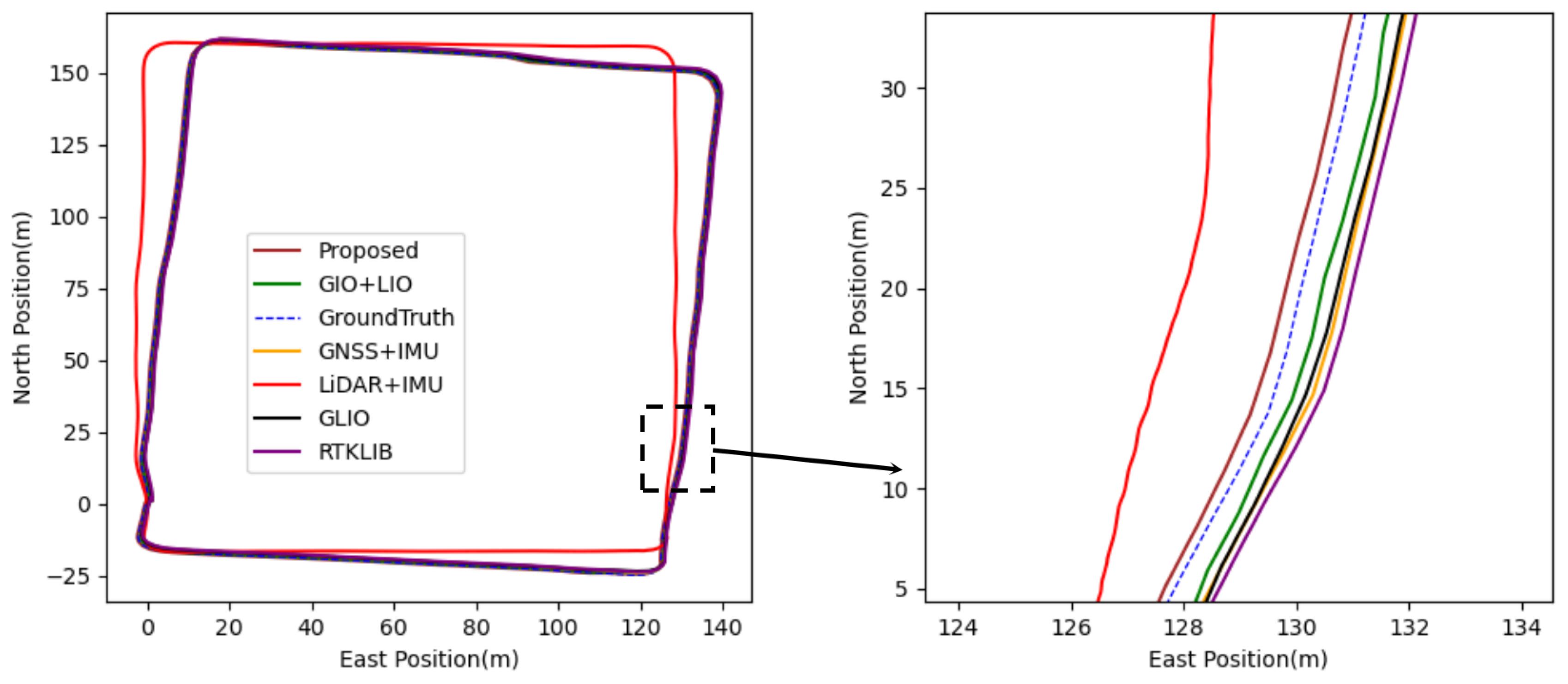
4.2.1. Testing of UrbanLoco

We selected two urban scenarios from the UrbanLoco dataset, HK0117 and HK0331, for the performance test, and the trajectory comparison is shown in Figure 5 and Figure 6.

Table 3. Positioning error comparison of different algorithms on the UrbanLoco HK0117 sequence.

	Horizontal Position Error (m)		Vertical Position Error (m)
	RMSE	Maximum Error	RMSE	Maximum Error
RTKLIB	1.99	5.47	6.14	12.02
GNSS+IMU	1.63	2.82	1.76	3.17
LiDAR+IMU	4.32	11.28	7.15	14.83
GIO+LIO	1.56	2.13	1.35	2.36
GLIO	1.61	2.55	1.13	2.93
Proposed	1.44	2.09	0.86	1.31

and

Table 4. Positioning error comparison of different algorithms on the UrbanLoco HK01331 sequence.

	Horizontal Position Error (m)		Vertical Position Error (m)
	RMSE	Maximum Error	RMSE	Maximum Error
RTKLIB	0.92	1.78	1.83	3.27
GNSS+IMU	1.29	2.02	0.94	1.61
LiDAR+IMU	18.78	30.60	1.69	2.65
GIO+LIO	1.31	1.72	1.49	1.93
GLIO	1.26	1.80	0.66	1.62
Proposed	0.88	1.64	0.75	1.38

, respectively, show the quantitative test results under the two scenarios, including Root Mean Square Error and maximum error. While RTKLIB demonstrates strong performance in horizontal positioning accuracy, it falls short in vertical positioning due to sudden shifts in error. This impacts the overall 3D position accuracy, rendering it less than ideal. This is primarily attributed to the multi-path interference triggered by high-rise buildings and city vehicles’ dynamic movement. In the HK0117 sequence, RTKLIB’s horizontal average error reaches up to 1.99 m, with the maximum spiking to 5.47 m; its vertical average error amounts to 6.14 m, with a maximum elevation of 12.02 m. Moving on to the HK0331 sequence, RTKLIB’s horizontal average error is marginally better at 0.92 m and a maximum error of 1.78 m. However, its vertical average error stands at 4.39 m, reaching a peak of 10.17 m. This data underscores a discernible deterioration of GNSS signal quality in the urban environment. The fusion of LiDAR and IMU within the odometry algorithm has been found to cause a degree of trajectory drift due to the accumulation of inherent errors. In the HK0117 sequence, the experiment revealed that the average and maximum errors in the horizontal plane were 4.32 m and 11.28 m, respectively. Regarding the vertical measurement, the average error was found to be 7.15 m, with a notable maximum discrepancy of 14.83 m. The HK0331 sequence presented an average error of 18.78 m in the horizontal plane and a significant maximum misalignment of 30.60 m. Conversely, the vertical error was tangibly lower, averaging 1.69 m and peaking at 2.65 m. The horizontal positioning error of the LIO odometry method is larger than that of GNSS sensor, although it maintains a more realistic trajectory shape.

When contrasted with the RTKLIB and LIO odometry approaches, the GNSS–IMU-based odometry significantly curtails pose error. Evaluations on the HK0117 sequence show that the horizontal average error for the GIO odometry is 1.63 m, with a maximum error of 2.82 m. The vertical average error clocks in at 1.76 m, with the maximum error reaching 3.17 m. For the HK0331 sequence, horizontal average error is observed at 1.29 m and the maximum at 2.02 m. The vertical errors average at 0.94 m, peaking at 1.61 m. As a result, the GNSS and IMU positioning combination is more prevalent in conventional settings. However, the odometry still registers a degree of error when there is substantial GNSS signal interference. This can be attributed to the inability of GNSS to receive high-precision positions and accurate covariance, thereby posing challenges for the graph optimizer.

In various scenarios, the performance of the loosely coupled GIO+LIO method fluctuates, exceeding or falling short of the GNSS+IMU odometry. In HK0117 sequence, this loosely coupled technique outperforms those relying solely on GNSS and IMU. The average horizontal error is reduced to 1.56 m, with a peak reduction to 2.13 m. Vertical errors average at 1.35 m, with a maximum error reported at 2.36 m. However, in the HK0331 sequence, errors resulting from loose-coupling emerge greater than with the GNSS+IMU odometry. The average horizontal error is calculated at 1.31 m, peaking at 1.72 m. Vertically, the average error stands at 1.49 m and reaches maximally 1.93 m. This can likely be attributed to the loosely coupled method’s inability to effectively balance the weights of the GIO and LIO odometry. If the trajectory drift of LIO odometry is excessive, the resultant error can come to compromise the whole loosely coupled system. This validation suggests that the loosely coupled approach may not be suitable for more complex environments.

Conclusively, our proposed method, reliant on multi-frame residuals and two-stage optimization, showcases superior performance. Upon analyzing the HK0117 sequence, the horizontal Root Mean Square Error is calculated to be 1.44 m, with a maximum error of 2.09 m. In terms of the vertical average error, it stands at 0.86 m, reaching a peak at 1.31 m. Proceeding to the HK0331 sequence assessment, the horizontal Root Mean Square Error decreases to 0.88 m, with the maximum error reducing to 1.64 m. The vertical average error is further reduced to 0.75 m, attaining a maximum error of 1.38 m. These results demonstrate the efficiency of the multi-frame residual factor in coordinating the error weights of GNSS, IMU, and LiDAR within the graph optimization system. Additionally, the secondary optimization strategy effectively mitigates the impact of faulty GNSS observations, resulting in an overall superior performance of the method.

Figure 5 and Table 3 also provide a comparative analysis of the GLIO and Proposed algorithms in terms of their trajectory accuracy and positioning errors on the UrbanLoco HK0117 sequence. In terms of trajectory accuracy, the Proposed method aligns more closely with the GroundTruth, displaying a smaller deviation, especially in the zoomed-in view, compared to GLIO, which shows noticeable deviations. For positioning errors, the Proposed method outperforms GLIO across all metrics. The horizontal position Root Mean Square Error (RMSE) for the Proposed method is 1.44 m, which is less than GLIO’s 1.61 m. Similarly, the maximum horizontal error of the Proposed method is 2.09 m, compared to 2.55 m for GLIO. In the vertical position error comparison, the Proposed method shows a significant improvement, with an RMSE of 0.86 m, while GLIO has an RMSE of 1.13 m. The maximum vertical error for the Proposed method is 1.31 m, considerably lower than GLIO’s 2.93 m.

On the UrbanLoco HK0331 sequence, the Proposed method shows a closer alignment to the GroundTruth, particularly noticeable in the zoomed-in view, where it displays smaller deviations compared to the GLIO algorithm. For positioning errors, the Proposed method consistently outperforms GLIO across all metrics. The horizontal position RMSE for the Proposed method is 0.88 m, which is lower than GLIO’s 1.26 m. The maximum horizontal error of the Proposed method is 1.64 m, compared to GLIO’s 1.80 m. In the vertical position error comparison, the Proposed method also demonstrates superior performance with an RMSE of 0.64 m, significantly lower than GLIO’s 0.66 m. The maximum vertical error for the Proposed method is 0.75 m, which is notably lower than GLIO’s 1.62 m.

Overall, these results highlight the superior performance of the Proposed tightly coupled GNSS/LiDAR/IMU integrated system with multi-frame residual factors, demonstrating its enhanced accuracy and reliability in trajectory optimization compared to the GLIO algorithm.

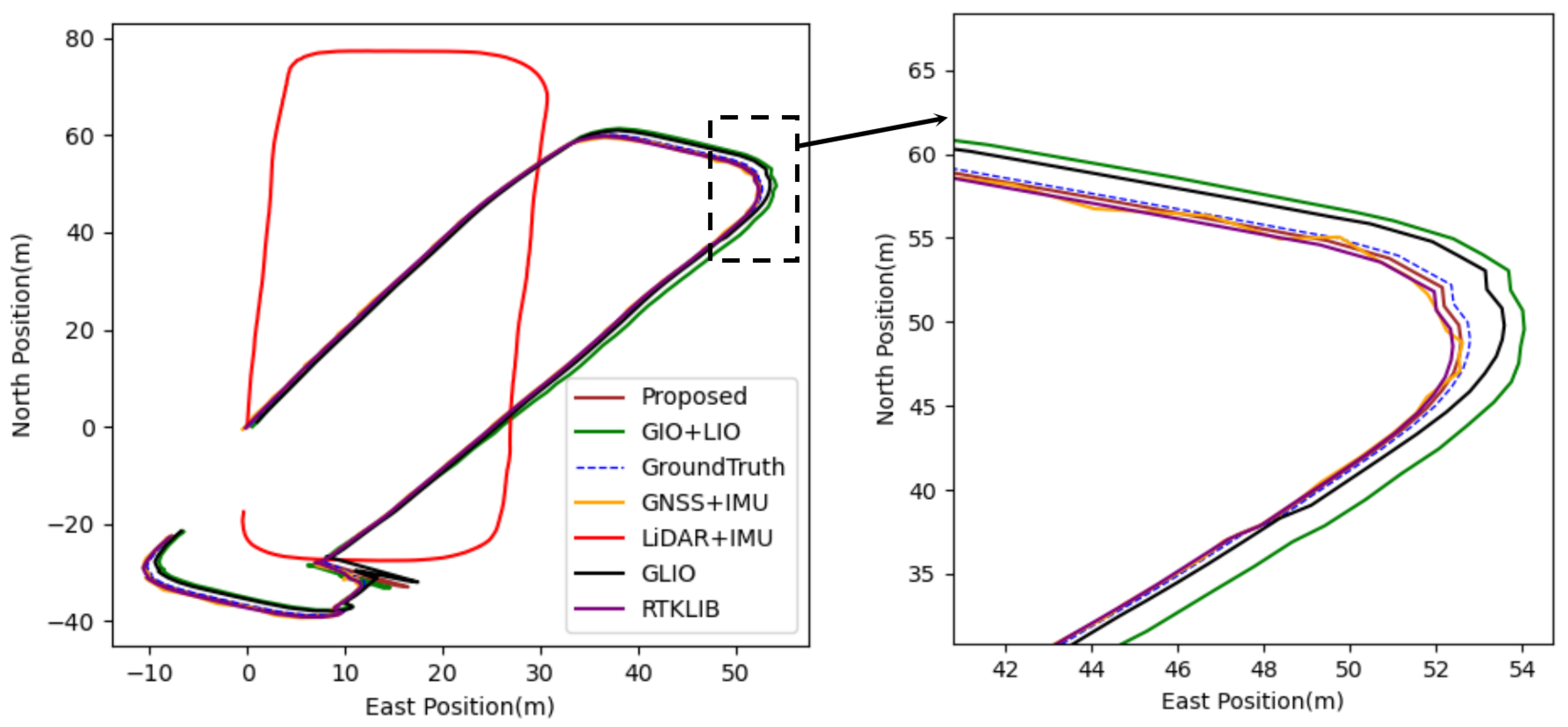
4.2.2. Testing of Actual Dataset

Figure 7 showcases the trajectories obtained from various algorithms, including the Proposed method, compared against the GroundTruth data. The table below (

Table 5. Positioning error comparison of different algorithms on an urban road scene.

	Horizontal Position Error (m)		Vertical Position Error (m)
	RMSE	Maximum Error	RMSE	Maximum Error
RTKLIB	3.59	4.86	2.63	9.44
GNSS+IMU	1.37	1.64	2.58	8.60
LiDAR+IMU	24.70	41.35	5.72	10.92
GIO+LIO	1.39	1.83	2.77	9.96
GLIO	1.08	1.69	1.39	3.23
Proposed	0.41	0.54	1.46	3.39

) presents the Root Mean Square Error (RMSE) and maximum errors in both horizontal and vertical positions.

The table clearly shows that the Proposed algorithm has the lowest horizontal position error among all the compared methods. The RMSE for the Proposed method is 0.41 m, significantly lower than the RTKLIB (3.59 m), GNSS+IMU (1.37 m), LiDAR+IMU (24.70 m), and GIO+LIO (1.39 m) methods. Additionally, the maximum horizontal error for the Proposed algorithm is only 0.54 m, which is in stark contrast to the maximum errors observed in other methods, with LiDAR+IMU being the highest at 41.35 m.

Similarly, the vertical position errors further demonstrate the advantage of the Proposed algorithm. It achieves an RMSE of 1.46 m, outperforming all other methods. For instance, RTKLIB and GNSS+IMU have RMSE values of 2.63 m and 2.58 m, respectively. The maximum vertical error for the Proposed method stands at 3.39 m, remarkably lower than the errors found with RTKLIB (9.44 m), GNSS+IMU (8.60 m), and GIO+LIO (9.26 m).

The trajectory plots in Figure 7 substantiate these numerical findings. The Proposed method’s trajectory aligns closely with the GroundTruth data, indicating higher positional accuracy. In contrast, other algorithms, especially LiDAR+IMU, show significant deviations from the GroundTruth trajectory.

Figure 8 displays the trajectories produced by different algorithms, including the Proposed method, against the GroundTruth data. The trajectories provide a visual representation that supports these quantitative findings. The Proposed method’s trajectory, though not perfect, remains closer to the GroundTruth data, indicating higher overall positional accuracy. In contrast, other algorithms show significant deviations, especially in areas with high environmental interference. As shown in

Table 6. Positioning error comparison of different algorithms on a school road scene.

	Horizontal Position Error (m)		Vertical Position Error (m)
	RMSE	Maximum Error	RMSE	Maximum Error
RTKLIB	7.27	30.54	7.92	13.65
GNSS+IMU	6.31	28.42	7.78	13.91
LiDAR+IMU	4.88	31.40	5.26	10.33
GIO+LIO	5.98	22.62	4.80	11.53
GLIO	4.75	27.99	3.51	8.84
Proposed	2.47	13.49	2.98	7.46

, the Proposed algorithm exhibits the lowest horizontal position error among all the evaluated methods. The RMSE for the Proposed method is 2.47 m, which, although higher than optimal, remains substantially lower than that of RTKLIB (7.27 m), GNSS+IMU (6.31 m), LiDAR+IMU (4.88 m), and GIO+LIO (5.98 m). The maximum horizontal error for the Proposed algorithm is 13.49 m, which is significantly lower compared to RTKLIB (30.54 m) and other methods.

The vertical position errors also affirm the advantage of the Proposed algorithm. It achieves an RMSE of 2.98 m, outperforming other methods such as RTKLIB and GNSS+IMU, which have RMSE values of 7.92 m and 7.78 m, respectively. The maximum vertical error for the Proposed method stands at 7.46 m, favorably lower than RTKLIB (13.65 m) and GNSS+IMU (13.91 m).

Given the environmental challenges such as weak GNSS signals and the high density of vehicles and pedestrians in the school area, achieving high positional accuracy is inherently difficult. These factors contribute to the performance degradation observed across all methods. Nevertheless, the Proposed algorithm’s superior performance demonstrates its robustness and adaptability in real-world, challenging conditions. The marginal errors associated with the Proposed method underscore its reliability compared to traditional algorithms under similar adverse circumstances.

The comparative analysis of the GLIO and Proposed algorithms on different datasets highlights the significant improvements achieved by the Proposed method. In both urban and school road scenes, the Proposed tightly coupled GNSS/LiDAR/IMU integrated system with multi-frame residual factors demonstrates superior trajectory accuracy, with closer alignment to GroundTruth and consistently lower positioning errors across all metrics compared to the GLIO algorithm. This clearly showcases the enhanced accuracy and robustness of the Proposed method in trajectory optimization.

Despite the challenging environment characterized by weak GNSS signals and significant disruptions due to vehicle and pedestrian activity, the Proposed algorithm exhibits superior performance in both horizontal and vertical positional accuracy. The analysis, reinforced by both statistical metrics and visual trajectory comparisons, validates the Proposed method’s effectiveness and reliability. This makes it a valuable solution for applications that require high positional accuracy in difficult environments.

We also focused on the system’s performance in mapping. By comparing the point cloud maps generated by LiDAR+IMU, GIO+LIO, and the proposed algorithm in a campus environment, we observed that the proposed algorithm demonstrated superior performance. From the top-down views (Figure 9), it is evident that the proposed algorithm offers more accurate and detailed structural integrity than the other two methods. The side views (Figure 10) further highlight the advantages of the proposed algorithm, showing minimal Z-axis drift, which is in sharp contrast to the vertical spreading observed in LiDAR+IMU and GIO+LIO. The original LIO odometry exhibited significant mapping errors in the complex campus environment. Although integrating GNSS assistance reduced Z-axis drift, it still resulted in inaccuracies in height mapping. This indicates that the proposed algorithm excels in maintaining vertical accuracy and stability, which is crucial for precise 3D environment reconstruction. Consequently, it proves to be highly effective and reliable for high-precision mapping applications.

5. Discussion

In this paper, we propose and validate the MFO-Fusion framework, which integrates GNSS, IMU, and LiDAR data to achieve high-precision positioning, even in challenging environments. Experimental results demonstrate that MFO-Fusion significantly outperforms existing fusion technologies under various complex conditions. Firstly, our experimental results show that multi-sensor fusion greatly enhances positioning accuracy compared to single-sensor systems. This improvement is particularly evident when GNSS signals are disrupted or lost. By combining the high-frequency short-term data from IMU with the environmental perception capabilities of LiDAR, MFO-Fusion effectively compensates for the shortcomings of individual sensors. Secondly, the use of a two-stage factor graph optimization strategy, based on multi-frame residual processing, further enhances the system’s robustness and accuracy. Compared to traditional optimization methods, the two-stage factor graph optimization strategy better handles nonlinear errors and offers greater flexibility and scalability in multi-sensor data fusion. Our experimental results also indicate that MFO-Fusion consistently demonstrates superior performance across different test environments. This suggests that our framework has strong generalization capabilities and can adapt to various complex real-world application scenarios. This result stands in stark contrast to previous studies, further proving the potential of multi-sensor fusion in improving positioning accuracy and robustness.

However, despite these significant advancements, MFO-Fusion has some limitations. For instance, the computational complexity is relatively high, and real-time performance needs further optimization. Additionally, in extreme environments such as severe occlusion or dynamic interference, the system’s performance still requires improvement. Future research could explore these areas further, including optimizing the computational efficiency of algorithms and incorporating more types of sensor data.

6. Conclusions

In this paper, we proposed and validated a novel framework called MFO-Fusion for sensor fusion and factor graph optimization in challenging environments. We provided a comprehensive description of the framework, including the multi-frame residual processing of GNSS/INS/LiDAR measurements and a two-stage factor graph optimization strategy. Through a series of experiments, we demonstrated the performance of MFO-Fusion in challenging environments and compared it with existing fusion techniques. The experimental results showed that MFO-Fusion significantly improves positioning accuracy, particularly in environments with limited GNSS signals. Compared to traditional methods, MFO-Fusion excels not only in fusing multiple sensors’ data but also in mitigating GNSS signal loss and the cumulative drift errors of other sensors. Furthermore, our research revealed potential directions for the further optimization of sensor fusion. Future research could focus on the following areas:

• Algorithm Optimization: Enhance the computational efficiency and robustness of factor graph optimization algorithms to adapt to more complex environments;
• Multi-Sensor Fusion: Explore the integration of additional sensors, such as visual sensors, to further improve positioning accuracy and environmental perception;
• Real-Time Applications: Develop real-time sensor fusion systems suitable for practical applications, such as autonomous driving and drone navigation.

In summary, the MFO-Fusion framework provides an effective solution for multi-sensor fusion in complex environments, offering broad application prospects and potential value. We look forward to more research and application explorations in this field to further enhance the performance and reliability of positioning and navigation technologies.

References

1. Cao, S.; Lu, X.; Shen, S. GVINS: Tightly coupled GNSS-visual-inertial fusion for smooth and consistent state estimation. IEEE Trans. Robot. 2022, 38, 2004–2021. [Google Scholar] [CrossRef]
2. Li, Y.; Zhuang, Y.; Hu, X.; Gao, Z.; Hu, J.; Chen, L.; El-Sheimy, N. Toward location-enabled IoT (LE-IoT): IoT positioning techniques, error sources, and error mitigation. IEEE Internet Things J. 2021, 8, 4035–4062. [Google Scholar] [CrossRef]
3. Qian, C.; Liu, H.; Tang, J.; Chen, Y.; Kaartinen, H.; Kukko, A.; Zhu, L.; Liang, X.; Chen, L.; Hyyppä, J. GNSS/INS/LiDAR-SLAM positioning method for highly accurate forest stem mapping. Remote Sens. 2017, 9, 3. [Google Scholar] [CrossRef]
4. Shan, T.; Englot, B.; Meyers, D. Lio-sam: Tightly-coupled lidar inertial odometry via smoothing and map. In Proceedings of the 2020 IEEE/RSJ International Conference on Intelligent Robots and Systems (IROS), Las Vegas, NV, USA, 24 October 2020–24 January 2021; pp. 5135–5142. [Google Scholar]
5. Barfoot, T.D. State Estimation for Robotics; Cambridge University Press: Cambridge, UK, 2017; pp. 205–284. [Google Scholar]
6. Crosara, L.; Ardizzon, F.; Tomasin, S. Worst-Case Spoofing Attack and Robust Countermeasure in Satellite Navigation Systems. IEEE Trans. Inf. Forensics Secur. 2023, 19, 2039–2050. [Google Scholar] [CrossRef]
7. Chang, J.; Zhang, Y.; Fan, S. An Anti-Spoofing Model Based on MVM and MCCM for a Loosely-Coupled GNSS/INS/LiDAR Kalman Filter. IEEE Trans. Intell. Veh. 2023, 9, 1744–1755. [Google Scholar] [CrossRef]
8. Radoš, K.; Brkić, M.; Begušić, D. Recent Advances on Jamming and Spoofing Detection in GNSS. Sensors 2024, 24, 4210. [Google Scholar] [CrossRef]
9. Chen, S.; Liu, B.; Feng, C.; Vallespi-Gonzalez, C.; Wellington, C. 3D Point Cloud Processing and Learning for AutonomousDriving: Impacting Map Creation, Localization, and Perception. IEEE Signal Process. Mag. 2020, 38, 68–86. [Google Scholar] [CrossRef]
10. Wang, Z.; Wu, Y.; Niu, Q. Multi-Sensor Fusion in Automated Driving: A Survey. IEEE Access 2019, 8, 2847–2868. [Google Scholar] [CrossRef]
11. Kim, H.; Lee, I. Localization of a car based on multi-sensor fusion. Int. Arch. Photogramm. Remote Sens. Spat. Inf. Sci. 2018, 42, 247–250. [Google Scholar] [CrossRef]
12. Wan, G.; Yang, X.; Cai, R.; Li, H.; Zhou, Y.; Wang, H.; Song, S. Robust and precise vehicle localization based on multi-sensor fusion in diverse city scenes. In Proceedings of the 2018 IEEE International Conference on Robotics and Automation, Brisbane, Australia, 21–25 May 2018; pp. 4670–4677. [Google Scholar]
13. Schütz, A.; Sánchez-Morales, D.E.; Pany, T. Precise positioning through a loosely-coupled sensor fusion of GNSS-RTK, INS and LiDAR for autonomous driving. In Proceedings of the 2020 IEEE/ION Position, Location and Navigation Symposium, Portland, OR, USA, 20–23 April 2020; pp. 219–225. [Google Scholar]
14. Martin, T. Advanced receiver autonomous integrity monitoring in tightly integrated GNSS/inertial systems. In Proceedings of the 2020 DGON Inertial Sensors and Systems, Braunschweig, Germany, 15–16 September 2020; pp. 1–14. [Google Scholar]
15. Li, T.; Pei, L.; Xiang, Y.; Wu, Q.; Xia, S.; Tao, L.; Yu, W. P 3-LOAM: PPP/LiDAR loosely coupled SLAM with accurate covariance estimation and robust RAIM in urban canyon environment. IEEE Sens. J. 2020, 21, 6660–6671. [Google Scholar] [CrossRef]
16. Qin, C.; Ye, H.; Pranata, C.E.; Han, J.; Zhang, S.; Liu, M. Lins: A LiDAR-inertial state estimator for robust and efficient navigation. In Proceedings of the 2020 IEEE International Conference on Robotics and Automation, Paris, France, 31 May 2020–31 August 2020; pp. 8899–8906. [Google Scholar]
17. Bai, S.; Lai, J.; Lyu, P.; Cen, Y.; Sun, X.; Wang, B. Performance Enhancement of Tightly Coupled GNSS/IMU Integration Based on Factor Graph with Robust TDCP Loop Closure. IEEE Trans. Intell. Transp. Syst. 2023, 25, 2437–2449. [Google Scholar] [CrossRef]
18. Jouybari, A.; Bagherbandi, M.; Nilfouroushan, F. Numerical Analysis of GNSS Signal Outage Effect on EOPs Solutions Using Tightly Coupled GNSS/IMU Integration: A Simulated Case Study in Sweden. Sensors 2023, 14, 6361. [Google Scholar] [CrossRef]
19. Wen, W. 3D LiDAR aided GNSS and its tightly coupled integration with INS via factor graph optimization. In Proceedings of the 33rd International Technical Meeting of the Satellite Division of the Institute of Navigation, Online, 21–25 September 2020; pp. 1649–1672. [Google Scholar]
20. Zhang, Z.; Liu, H.; Qi, J.; Ji, K. A tightly coupled LiDAR-IMU SLAM in off-road environment. In Proceedings of the 2019 IEEE International Conference on Vehicular Electronics and Safety, Cairo, Egypt, 21 November 2019; pp. 1–6. [Google Scholar]
21. Pan, H.; Liu, D.; Ren, J.; Huang, T.; Yang, H. LiDAR-IMU Tightly-Coupled SLAM Method Based on IEKF and Loop Closure Detection. IEEE J. Sel. Top. Appl. Earth Obs. Remote Sens. 2024, 17, 6986–7001. [Google Scholar] [CrossRef]
22. Dellaert, F. Factor graphs and GTSAM: A hands-on introduction. Ga. Inst. Technol. 2012, 2, 4. [Google Scholar]
23. Hu, G.; Wang, W.; Zhong, Y. A new direct filtering approach to INS/GNSS integration. Aerosp. Sci. Technol. 2018, 77, 755–764. [Google Scholar] [CrossRef]
24. Wu, Y.; Wang, J.; Hu, D. A new technique for INS/GNSS attitude and parameter estimation using online optimization. IEEE Trans. Signal Process. 2014, 62, 2642–2655. [Google Scholar] [CrossRef]
25. Dai, H.; Bian, H.; Wang, R. An INS/GNSS integrated navigation in GNSS denied environment using recurrent neural network. Def. Technol. 2020, 16, 334–340. [Google Scholar] [CrossRef]
26. Abdelaziz, N.; El-Rabbany, A. An integrated ins/lidar slam navigation system for gnss-challenging environments. Sensors 2022, 22, 4327. [Google Scholar] [CrossRef] [PubMed]
27. Tang, J.; Chen, Y.; Niu, X. LiDAR scan matching aided inertial navigation system in GNSS-denied environments. Sensors 2015, 15, 16710–16728. [Google Scholar] [CrossRef]
28. Xu, W.; Zhang, F. FAST-LIO: A Fast, Robust LiDAR-Inertial Odometry Package by Tightly-Coupled Iterated Kalman Filter. IEEE Robot. Autom. Lett. 2021, 6, 3317–3324. [Google Scholar] [CrossRef]
29. Chen, H.; Wu, W.; Zhang, S.; Wu, C.; Zhong, R. A GNSS/LiDAR/IMU Pose Estimation System Based on Collaborative Fusion of Factor Map and Filtering. Remote Sens. 2023, 3, 790. [Google Scholar] [CrossRef]
30. Li, S.; Li, X.; Zhou, Y.; Xia, C. Targetless extrinsic calibration of LiDAR-IMU system using raw GNSS observations for vehicle applications. IEEE Trans. Instrum. Meas. 2023, 72, 1003311. [Google Scholar] [CrossRef]
31. Zhang, J.; Wen, W.; Huang, F.; Chen, X.; Hsu, L.T. Continuous GNSS-RTK aided by LiDAR/inertial odometry with intelligent GNSS selection in urban canyons. In Proceedings of the 34th International Technical Meeting of the Satellite Division of the Institute of Navigation, St. Louis, MO, USA, 20–24 September 2021; pp. 4198–4207. [Google Scholar]
32. Liu, T.; Li, B.; Yang, L.; He, L.; He, J. Tightly coupled gnss, ins and visual odometry for accurate and robust vehicle positioning. In Proceedings of the 2022 5th International Symposium on Autonomous Systems, Hangzhou, China, 22 April 2022; pp. 1–6. [Google Scholar]
33. Li, X.; Wang, S.; Li, S.; Zhou, Y.; Xia, C.; Shen, Z. Enhancing RTK Performance in Urban Environments by Tightly Integrating INS and LiDAR. IEEE Trans. Veh. Technol. 2023, 8, 9845–9856. [Google Scholar] [CrossRef]
34. Bai, S.; Lai, J.; Lyu, P.; Wang, B.; Sun, X.; Yu, W. An Enhanced Adaptable Factor Graph for Simultaneous Localization and Calibration in GNSS/IMU/Odometer Integration. IEEE Trans. Veh. Technol. 2023, 9, 11346–11357. [Google Scholar] [CrossRef]
35. Pan, L.; Ji, K.; Zhao, J. Tightly-coupled multi-sensor fusion for localization with LiDAR feature maps. In Proceedings of the 2021 IEEE International Conference on Robotics and Automation, Xi’an, China, 18 October 2021; pp. 5215–5221. [Google Scholar]
36. Lee, J.U.; Won, J.H. Adaptive Kalman Filter Based LiDAR aided GNSS/IMU Integrated Navigation System for High-Speed Autonomous Vehicles in Challenging Environments. In Proceedings of the 2024 International Technical Meeting of The Institute of Navigation, Long Beach, CA, USA, 23–25 January 2024; pp. 1095–1102.
37. Ai, M.; Asl Sabbaghian Hokmabad, I.; Elhabiby, M.; El-Sheimy, N. A novel LiDAR-GNSS-INS Two-Phase Tightly Coupled integration scheme for precise navigation. ISPRS Ann. Photogramm. Remote Sens. Spat. Inf. Sci. 2024, 10, 1–6. [Google Scholar] [CrossRef]
38. Shen, Z.; Wang, J.; Pang, C.; Lan, Z.; Zheng, Y.; Fang, Z. A LiDAR-IMU-GNSS fused mapping method for large-scale and high-speed scenarios. Measurement 2024, 225, 113976. [Google Scholar] [CrossRef]
39. Gao, J.; Sha, J.; Li, H.; Wang, Y. A Robust and Fast GNSS-Inertial-LiDAR Odometry With INS-Centric Multiple Modalities by IESKF. IEEE Trans. Instrum. Meas. 2024, 73, 8501312. [Google Scholar] [CrossRef]
40. Liu, X.; Wen, W.; Hsu, L.T. GLIO: Tightly-Coupled GNSS/LiDAR/IMU Integration for Continuous and Drift-free State Estimation of Intelligent Vehicles in Urban Areas. IEEE Trans. Intell. Veh. 2023, 1, 1412–1422. [Google Scholar] [CrossRef]
41. Noureldin, A.; Karamat, T.B.; Georgy, J. Fundamentals of Inertial Navigation, Satellite-Based Positioning and Their Integration; Springer Science + Business Media: Berlin, Germany, 2012; pp. 65–123. [Google Scholar]
42. Crassidis, J.L. Sigma-point Kalman filtering for integrated GPS and inertial navigation. IEEE Trans. Aerosp. Electron. Syst. 2006, 42, 750–756. [Google Scholar] [CrossRef]
43. Vijeth, G.; Gatti, R.R. Review on Robot Operating System. Self-Powered Cyber Phys. Syst. 2023, 297–307. [Google Scholar] [CrossRef]
44. Wen, W.; Zhou, Y.; Fahandezh-Saadi, S.; Bai, X.; Zhan, W.; Tomizuka, M.; Hsu, L.T. UrbanLoco: A Full Sensor Suite Dataset for Mapping and Localization in Urban Scenes. In Proceedings of the 2020 IEEE International Conference on Robotics and Automation (ICRA), Paris, France, 15 September 2020; pp. 2310–2316. [Google Scholar]
45. Vázquez-Ontiveros, J.R.; Padilla-Velazco, J.; Gaxiola-Camacho, J.R.; Vázquez-Becerra, G.E. Evaluation and Analysis of the Accuracy of Open-Source Software and Online Services for PPP Processing in Static Mode. Remote Sens. 2023, 15, 2034. [Google Scholar] [CrossRef]
Figure 1. Sensor fusion and optimization pipeline. The pipeline begins with sensor data reading and processing, where GNSS measurements are preprocessed, IMU data undergo pre-integration, and point clouds are used for initialization and keyframe selection. This is followed by factor modeling, converting GNSS data to GNSS pseudorange factors, IMU data to IMU pre-integration factors, and LiDAR data to LiDAR odometry factors. In the first stage of optimization, GNSS and IMU factors pass through factor graph optimization to produce GIO and LIO poses. Finally, in the second stage of optimization, multi-frame residual factors and factor graph optimization refine the global pose.
Remotesensing 16 03114 g001
Figure 2. The two-stage optimization process for sensor fusion using GNSS, IMU, and LiDAR data. The first stage integrates GNSS pseudorange, IMU pre-integration, and LiDAR odometry factors to estimate initial states. The second stage refines these estimates with additional multi-frame residual factors for improved accuracy.
Remotesensing 16 03114 g002
Figure 3. Various scenarios in the experimental field. The red line trajectory represents the urban road scene, and the blue line trajectory area represents the campus scene. In both areas, the trajectory passes through an environment shielded by trees and buildings, leading to satellite signal interference.
Remotesensing 16 03114 g003
Figure 4. Experimental equipment setup for data collection.
Remotesensing 16 03114 g004
Figure 5. Trajectory comparison of different algorithms on the UrbanLoco HK0117 sequence. The image has been modified.
Remotesensing 16 03114 g005
Figure 6. Trajectory comparison of different algorithms on the UrbanLoco HK0331 sequence. The image has been modified.
Remotesensing 16 03114 g006
Figure 7. Trajectory comparison of different algorithms on an urban road scene. The image has been modified.
Remotesensing 16 03114 g007
Figure 8. Trajectory comparison of different algorithms on a school road scene. The image has been modified.
Remotesensing 16 03114 g008
Figure 9. Generated top views of the campus environment point cloud under different algorithms. The brightness of the point cloud represents the position height of the point cloud.
Remotesensing 16 03114 g009
Figure 10. Generated side view of the campus environment point cloud. This view clearly shows the Z-axis drift of the map under different algorithms.
Remotesensing 16 03114 g010