The Observation of Traveling Ionospheric Disturbances Using the Sanya Incoherent Scatter Radar

Abstract

In this study, we used the Sanya Incoherent Scatter Radar (SYISR) to observe the altitude profiles of traveling ionospheric disturbances (TIDs) during a moderate magnetic storm from 13 to 15 March 2022. Three TIDs were recorded, including two large-scale TIDs (LSTIDs) and one medium-scale TID (MSTID). These LSTIDs occurred during the storm recovery phase, characterized by periods of ~110–155 min, downward phase velocities of 22–60 m/s, and a relative amplitude of 17–25%. A nearly vertical front was noted at ~350–550 km, differing from AGW theory predictions. This structure is more attributed to the combined effects of sunrise-induced electron density changes and pre-sunrise uplift. Moreover, GNSS observations linked this LSTID to high-latitude origins, indicating a connection to polar magnetic storm excitation. However, the second LSTID was observed at lower altitudes (150–360 km) with a higher elevation angle (~17°). This LSTID, observed by the SYISR, was absent in the GNSS data from mainland China and Japan, suggesting a potential local source. The MSTID exhibited a larger relative amplitude of 29–36% at lower altitudes (130–210 km) with severe upward attenuation. The MSTID may be related to atmospheric gravity waves from the lower atmosphere. AGWs are considered to be the perturbation source for this MSTID event.

1. Introduction

Large-scale traveling ionospheric disturbances (LSTIDs) generally manifest as atmosphere gravity waves (AGWs) that are triggered around the auroral region [1]. These LSTIDs can propagate over several thousand kilometers. LSTIDs experience larger dissipation at low latitude than at mid- and high latitudes [2,3]. Unnikrishnan et al. [4] observed rapid equatorward LSTID decay during magnetic storms south of 35°N at ~−1 TECU/100 km. The accelerated decay of low-latitude LSTIDs may result from increased dissipation, including ion drag due to increased electron density in these areas [5,6,7]. Liu and Yeh [8] reported that the attenuation of AGWs caused by ion drag is modulated by the magnetic inclination and magnetic declination of the geomagnetic field. The attenuation is weaker when AGWs move along the magnetic lines of force. Moreover, some studies suggest that TID amplitude decay only partially reflects AGW decay, and the horizontal decay of LSTIDs increases proportionally with an increase in the elevation angle of an AGW [6,9].

Observations reveal some differences in LSTID propagation directions between low and high latitudes. Most of the LSTIDs exhibited a southwestward propagation direction in the Northern Hemisphere. At low latitudes, although the propagation azimuth of LSTIDs exhibits considerable variability among individual cases, statistical studies have shown a westward deflection with an average angle of ~17°–30° from the south [10]. This westward deflection is more obvious at low latitudes than at mid-latitudes (~9°–20°) [6,11] and high latitudes (i.e., ~4–7°) [12]. Some authors have suggested that latitudinal variation in propagation direction originates from the cumulative effect of the Coriolis force during the long-distance propagation of AGWs [13,14].

The multi-wave structures of LSTIDs are another notable feature observed at low latitudes. Previous studies have demonstrated that LSTIDs originating from the north and south polar regions are often observed simultaneously at low latitudes during magnetic storms, and they exhibit a multi-wave structure [15,16]. In the low-latitude regions of the Northern Hemisphere, poleward LSTIDs from the Southern Hemisphere typically exhibit smaller amplitudes due to increased dissipation during cross-equatorial propagation [17]. These multi-wave structures consist of simultaneous wavefronts from various directions at different velocities, resulting in overlapping peak amplitudes of differential total electron content (DTEC) [16]. Jacobson et al. [18] reported that multi-wave processes are active simultaneously in different seasons and weather conditions, predominantly propagating east and southeast. Recent studies suggest that the composition of multi-wave structures at low latitudes may result from various excitation sources beyond polar origins, including the enhanced equatorial electrojet (EEJ) during magnetic storms, secondary gravity waves due to primary gravity wave dissipation in the troposphere, and solar terminator effects [19,20,21]. Solar terminator effects are disturbances in the atmosphere and ionosphere caused by the rapid transition from day to night at the boundary at sunrise and sunset.

While the horizontal evolution characteristics of LSTIDs have been investigated extensively, limited observations have been conducted to assess the vertical propagation features of LSTIDs. Thome [22] used incoherent scatter radar (ISR) measurements over Puerto Rico and observed that the dominant period of gravity waves (GWs) increases with height, which may be related to fluctuations in background density and wind fields. Consistent findings were noted by Harper and Woodman [23] for the Jicamarca ISR within an altitude range of 60–80 km. Sterling et al. [24] combined ISR and ionosonde data and suggested that variations in the dominant period of internal gravity waves (IGWs) between mid-latitudes and extremely low latitudes may originate from ducted propagation mechanisms. Studies by Bertin et al. [25] and Vlasov et al. [26] revealed that AGWs were most clearly observed in ion line-of-sight velocities, while other parameters exhibited more oscillatory behavior, possibly influenced by polar energy injection. Oliver et al. [27] observed that F-layer TIDs typically have vertical wavelengths ranging from tens of km to 200 km. Moreover, the vertical phase velocities of LSTIDs increase with altitude and decrease with period [28,29,30]. Observations conducted by Djuth et al. [31] revealed that the multi-wave characteristics of GW perturbations manifest in vertical observations with different vertical phase velocities. However, weaker GW components may carry a large amplitude. This results in the multi-wave structure displaying dominant band-like patterns accompanied by some small-scale quasi-periodic downward-propagating oscillatory structures on the electron density perturbation map. However, the vertical propagation features of LSTIDs at low latitudes have not been comprehensively studied thus far due to the limited distribution and operational time of ISRs; furthermore, less emphasis has been placed on studying neutral atmosphere dynamics.

The Sanya Incoherent Scatter Radar (SYISR), which has been in operation since 2021, is currently available for ionospheric observation experiments at low latitudes. The high transmission power and multiple waveforms of the SYISR allow it to obtain profiles with high-precision ionospheric parameters, including electron density and electron temperature. This capability effectively fulfills the requirement for investigating the vertical features of LSTIDs. In this study, we investigated the development of LSTIDs during a moderate magnetic storm from 13 to 15 March 2022, using the SYISR. We also combined total electron content (TEC) data from the GNSS network to examine the propagation process of LSTIDs at low latitudes.

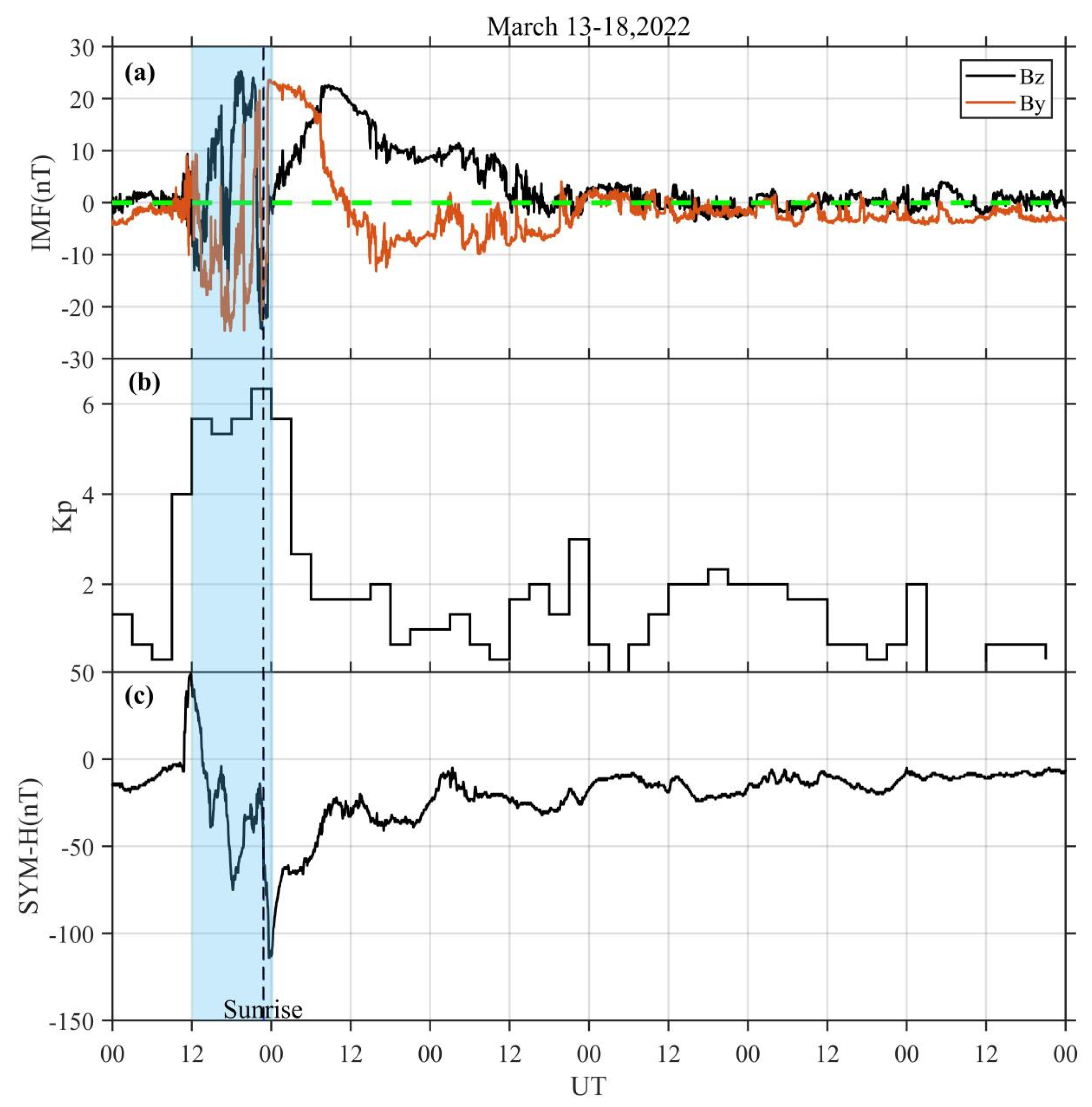
2. Geomagnetic Activity

From 13 to 18 March 2022, a moderate-intensity geomagnetic storm occurred after coronal mass ejections (CMEs) on 10 March. Geospace conditions were monitored using the measurements of the interplanetary magnetic field (IMF) in the Geocentric Solar Ecliptic (GSE) coordinate system, the Kp index, and the SYM-H index, as shown in Figure 1. The IMF data were observed by Advanced Composition Explorer (ACE, Explorer 71). Under the IMF shock, the Bz index exhibited three southward turns between ~11:00 UT on 13 March and 00:00 UT on 14 March (Figure 1a). Throughout these reversals, the Kp index maintained a high level, ranging from 5.3 nT to 6.3 nT (Figure 1b). The SYM-H index rapidly increased from −7 nT to 49 nT within 46 min after 10:45 UT on 13 March, indicating the sudden commencement (SSC) of the magnetic storm (Figure 1c). Subsequently, the SYM-H index decreased as the magnetic storm entered the main phase, reaching a minimum value of −114 nT at ~23:40 UT. During the main phase, local minima of −17.29 nT and −75 nT were observed at ~14:55 UT and 18:12 UT, respectively. After ~23:40 UT, all indices gradually returned to quiet-period levels, and the SYM-H index increased to above −20 nT after 02:00 UT on 15 March, indicating quiet conditions.

3. Materials and Methods

In this study, we use the SYISR to observe the vertical variation in LSTIDs during magnetic storms. To evaluate the horizontal features of the LSTIDs, TEC measurements derived from GNSS network stations were also used. The locations of the SYISR and GNSS stations are shown in Figure 2.

From 2015 to 2020, with the support of the National Natural Science Foundation of China (NSFC), a phased-array incoherent scatter radar was built in Sanya (109.6°E, 18.3°N; Dip 12.8°N). The radar consists of 4096 antennas and transmit/receive (T/R) units with a peak transmission power greater than 2 MW and a maximum antenna gain of 43 dBi [32]. The SYISR employs solid-state transmitters and digital receivers. It is also equipped with various waveforms, including Barker codes (BCs), long pulses (LPs), and alternating codes (ACs). The powerful detection capabilities of the SYISR make it a powerful ground-based device for detecting the upper atmosphere in modern phased array systems at low latitudes in Asia.

During the 13–15 March 2022 magnetic storm, the SYISR continuously operated in zenith stare mode (a single beam) using a 13-bit BC, with a pulse width of 390 $\mathsf{\mu }\mathrm{s}$ and a duty cycle of ~4.9%. The technical indices of the SYISR included a peak power exceeding 2 MW, an antenna gain of 43 dBi, and a noise temperature below 120 K. Compared to other waveforms (e.g., AC and LP), the BC has the characteristics of zero autocorrelation and a low sidelobe, resulting in a higher range resolution [33]. In signal processing, the echo signal detected by the BC was convolved with a matched filter to obtain a signal that effectively improves the height resolution [34]. To eliminate the effects of noise and clutter, incoherent accumulation was performed on the pulse-compressed signal, yielding the power spectrum of the squared signal. According to the radar equation, the ionospheric electron density is proportional to the power of the radar echo signal [35]. Based on this principle, we obtained the altitude profiles and temporal variations in the electron density. Finally, we decoded the raw electron density from the radar equation with a spatial resolution of ~4.5 km and a temporal resolution of ~0.8 s at an altitude ranging from 80 to 1100 km [36].

In this study, TEC data observed by ground-based dual-frequency (f1 = 1.57542 GHz, f2 = 1.2266 GHz) GNSS networks in the Chinese region were also used. These data were provided by the China Meteorological Administration (CMA). Carrier phase and group delay data with temporal resolutions of 15 s and 30 s were recorded at 917 GPS receiving stations. Assuming a thin layer approximation and setting the ionospheric penetration point (IPP) height to 375 km, we applied a mapping function to convert these data to vertical TEC (vTEC) [37]. To avoid multipath errors and ionospheric masking effects, only observations with elevation angles exceeding 30° were considered. In this paper, differential TEC (DTEC) was obtained by applying a bandpass filter of 10–150 min, and 2D-TEC maps were derived from the DTEC. To derive the horizontal parameters of TID events, a slice (the green arrow in Figure 2) was set along the direction of vertical TID propagation to calculate the time–distance plot of TEC perturbations (keogram map). The slice direction, perpendicular to TIDs, enhances clarity for quantitative analyses. The source point of the slice was set at 47.7°5°E (marked by the yellow dot in Figure 2) for detailed representation and facilitated analysis, as outlined by Chen et al. [16].

4. Results

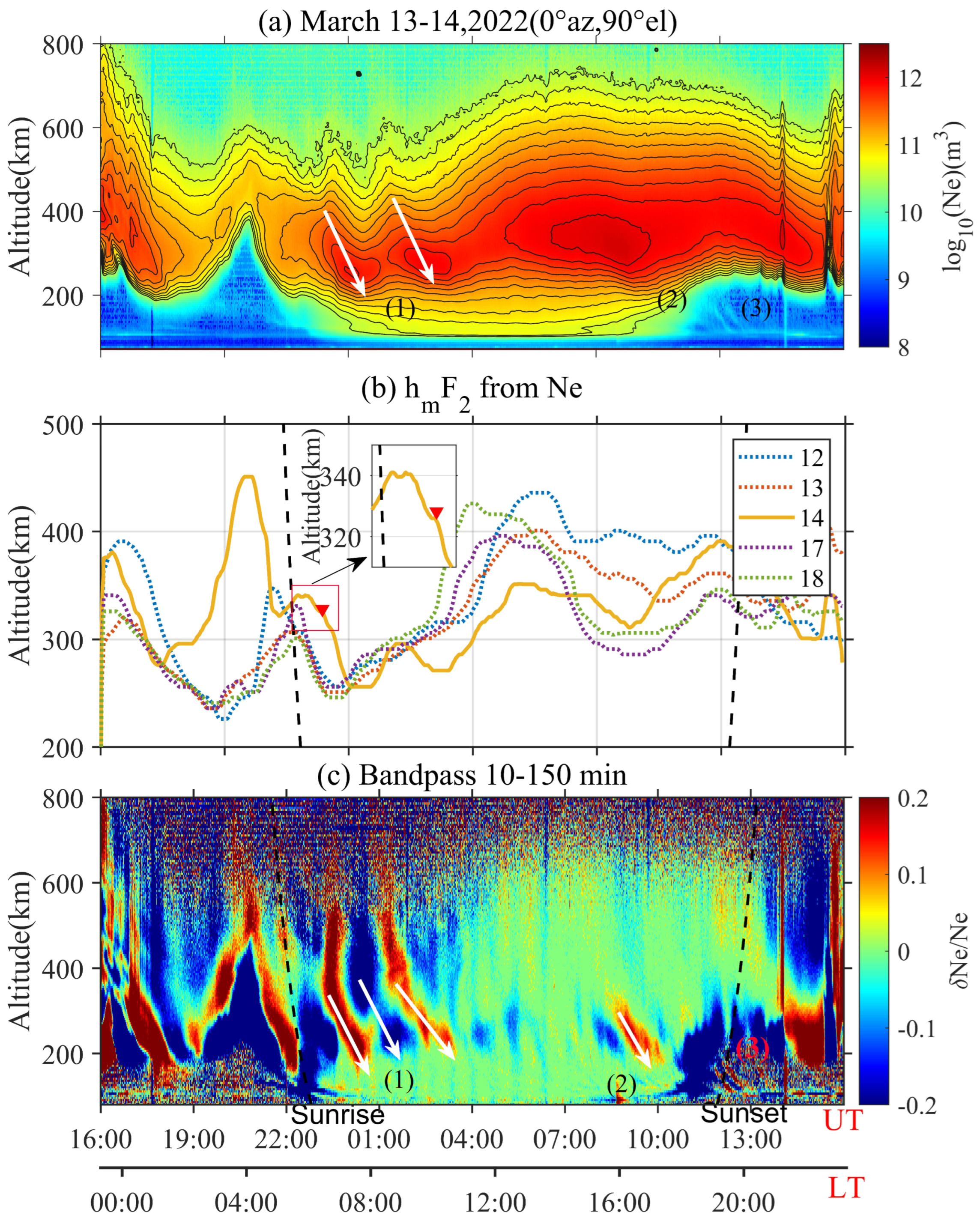
4.1. Result from SYISR

Figure 3a shows the electron density profiles observed by the SYISR in the zenith direction during the period from 16:00 on 13 March to 16:00 UT on 14 March. A diurnal variation is observable in Figure 3a, which shows a post-sunrise increase in electron density with a peak at ~13:00 LT and a gradual decrease after sunset. Between ~10:00UT and 12:00UT, a sharp increase in electron density was observed at altitudes ranging from 105 to 115 km, and this increase was identified as the ionospheric sporadic E-layer (Es layer). Subsequently, as shown in Figure 3a, a discontinuous disturbance structure was observed between 14:00 UT and 16:00 UT on 14 March (~21:20 and 23:20 LT), corresponding to the spread-F events observed in the frequency–height map of the Sanya region. This may be attributed to nighttime plasma bubbles or blobs. Such sudden and intense disturbances in electron density are a common feature at night, occurring on both quiet and disturbed days in low latitudes, and are consistent with previous observations [38,39].

In Figure 3b, the F-layer peak heights derived from the ISR observations of electron density on the days before and after 14 March are presented. Based on our experiments, a positive storm occurred at low latitudes, leading to an increase in ionosphere peak height effects between 19:00 and 22:00 UT (~02:20 and 05:20 LT) on 13 March. Furthermore, according to Figure 3a,b, a regular pre-sunrise uplift was observed between ~20:53 and 23:24 UT (~04:18 and 07:04 LT) on 13 March. This uplift with a lower velocity of ~14.5 m/s resulted in variations in the ionosphere at ~21:50 UT–22:40 UT (~05:10–06:00 LT). This uplift, with a velocity of ~14.5 m/s, causes the peak height of the ionospheric layer to increase to 300–352 km. The nighttime ionospheric enhancement on magnetic quiet days at low latitude is usually considered to be related to plasma transport processes, which mainly include a combination of ambipolar diffusion, neutral winds, and $\overrightarrow{E}\times \overrightarrow{B}$ [40,41]. The pre-sunrise uplift process is associated with a decrease in the electric field at night. The neutral wind during 00:00–05:00 LT usually lifts the ionosphere through equatorward wind. After 02:00LT, the weakening electric field or reversal of $\overrightarrow{E}\times \overrightarrow{B}$ drift may fail to offset the combined upward force of neutral winds and diffusion, resulting in pre-sunrise ionospheric uplift [36]. Furthermore, influenced by the weakening electric field during the storm, particularly between ~19:30 and 23:03 UT (~02:50 and 06:23 LT) on 13 March, the pre-sunrise uplift elevated the ionosphere at speeds of ~14.5 and 25 m/s to altitudes of 341–451 km, surpassing quiet-time uplift levels (Figure 3b).

A 10–150 min bandpass filter was applied to each Ne time series to obtain the disturbance dNe. The relative variation was then derived by dividing dNe by the background Ne0, as shown in Figure 3c. The lower and upper boundaries of the moving windows were selected based on both the existing knowledge of the common range of periods of TIDs and the estimation of periods from the raw data. The altitude range in which the signal-to-noise ratio (SNR) is sufficient to support our clear observation of the electron density variation is from 85 km to 800 km. Above 800 km, perturbations are not observable due to the weak echo signals and reduced SNR. For the same reason, the results are not valid below ~85 km. During the observation period, three quasi-periodic variations displaying downward phase progression were identified. These variations are attributed to TID events. Figure 3c shows that two LSTIDs can be observed at 23:00–03:30 UT and 8:30–10:15 UT. During the nighttime on 14 March, a medium-scale TID (MSTID) occurred from 11:40 to 12:50 UT (~19:00 to 20:10 LT) at the bottom of the ionosphere. The band-like structure observed from approximately 16:30 UT to 22:00 UT on 13 March, reflecting the positive storm effects on filtered ionospheric changes, is beyond the scope of TID-focused discussion.

The first LSTID event began before sunrise at ~22:50 UT (~06:10 LT) on 13 March and lasted for ~5 h (Figure 3c). This event was characterized by two positive phase fronts and one negative front with amplitudes of 18–25%, displaying a large range of quasi-periodic oscillations in electron density (Figure 3a,c). The phase fronts extend from ~180 km to more than 700 km. The average period and average vertical phase velocity of the TID were derived from the intervals and slopes of the positive phase front, resulting in values of ~143.5 ± 11.8 min and ~−50.1 ± 10.2 m/s, respectively. Negative values of velocity indicate downward propagation. The second TID event involved a shorter vertical phase velocity of 31.5 ± 8.9 m/s. This TID was observed at a lower altitude range of ~150–360 km with a weak amplitude of ~17–20% and a half period of 55 min on 14 March, exhibiting solitary waves. Unlike the first event, the amplitude of the second LSTID event rapidly decreased with increasing altitude, attenuating to below ~2.1% at ~350 km. This finding indicates a significantly smaller height coverage than that of the first LSTID event.

As shown in Figure 3c, the third TID with a period of 32.2 ± 2.1 min, was observed from 12:00 to 14:00 UT (~19:20 to 21:20 LT) after nightfall on 14 March. This MSTID event was identified by a strong amplitude at ~130 km altitude and significant vertical dissipation. The amplitude ranged from ~ 29% to 36%. This value surpassed the maximum amplitude of the first two LSTID events (i.e., 18–25%). The amplitude of the MSTID decreased quickly as it moved upwards and nearly disappeared upon reaching an altitude of ~210 km.

To show the vertical variation in these TIDs more clearly, we present the temporal perturbation series $\delta Ne/Ne$ at different altitudes in Figure 4. As shown in Figure 4a, the first TID can be observed between 180 and 700 km. The amplitude increased from 11% at 180 km to 29% at 480 km and then decreased above 480 km. The second LSTID event, as depicted in Figure 4b, occurred at a lower altitude range of 170–380 km, with a peak amplitude of ~20% at 250 km. Compared to the first LSTID event, the second LSTID event affected the ionosphere with a weaker amplitude over a narrower altitude range. The third TID event demonstrated a continuous decrease in amplitude with increasing altitude, decreasing by ~−1.11% per kilometer between 130 km and 210 km.

Notably, even though the two phase fronts of the first TID observed by the SYISR (Figure 3c and Figure 4a) originated from the same event, the first phase front is more vertical in the top ionosphere. Previous ISR observations suggested that the phase of atmospheric gravity waves (AGWs) tends to become nearly vertical above 400 km due to the influence of background viscosity on their upward propagation [42]. However, such background variations are insufficient to account for the short-term changes in the phase front. The anomaly phase is observed during 23:00–00:00 UT on 13 March. The front seems to show an almost vertical phase propagation at an altitude ranging from ~350 km to 550 km. Further analysis revealed that this observed phase anomaly is closely related to ionosphere disturbances caused by the combined effect of sunrise and pre-sunrise uplift rather than by variations in the AGW. The unusual phase front occurred between ~06:20 and 09:10 LT (~23:06 and 01:26 UT) shortly after local sunrise (~06:10 LT). In response to sunrise, the electron density at lower altitudes increases more rapidly than that at higher altitudes. Simulations suggest a shift from photochemical dominance at low altitudes to transport processes at higher altitudes [43,44]. The model results indicate that the maximum altitude of electron density variation caused by sunrise shifts to higher altitudes over time [45]. Multiple days of SYISR observations reveal a time delay of ~36–45 min between the increase in electron density at 181 km and 320 km altitude during quiet magnetic days. The electron density variations induced by sunrise at different altitudes result in an almost vertical phase in the electron density time series at different altitudes. This phase was mixed with the phases generated by TIDs at different altitudes, resulting in the observed phase anomaly shown in Figure 3c and Figure 4a. Moreover, during this magnetic disturbance period, the ionosphere during the corresponding period of the first TID event was lifted by ~40–70 km relative to that during the same period on a quiet day (22:50 UT–23:35 UT; Figure 3b). Under the combined influence of sustained electric field disturbances and sunrise, the ionosphere is lifted to higher altitudes. The continued increase in electron density corresponded to the increase in the altitude of the phase anomaly during the first TID event, suggesting an interaction with TID-induced changes and contributing to the observed phase anomaly in the filtered observations (Figure 3c and Figure 4a).

4.2. Result from GNSS TEC

To investigate the horizontal propagation characteristics of these TIDs, we utilized dense GNSS data from the Chinese regional network to analyze the 2D-TEC variations in TIDs in China, as illustrated in Figure 5. The results revealed three groups of LSTID events (group A, group B, and group C) during this period. Among them, the A group of TIDs, which was observed after sunrise (~06:20 LT), propagated westward (see the phase fronts plotted with dashed lines). TID events with similar directions during the same local time were also observed on both the preceding and following days, which implies that the first group of TIDs is caused by the solar terminator (ST), which are commonly observed in the Chinese region [13].

The black solid line in Figure 6 represents the phase lines of the group B TID events. These TIDs propagated southeastward with an azimuth of ~169° to 172°. The keogram shown in Figure 6 provides detailed information on the components of the propagation of these TIDs. The wavefronts in the keogram formed nearly continuous lines, exhibiting well-organized periodicity with an average period of 136.2 ± 11.8 min, which is consistent with the first TID event observed by the SYISR. The first two persistent positive fronts, moving at a horizontal velocity of 587.14 ± 71.11 m/s, cover an extensive region exceeding 3500 km in the slice shown (Figure 1). After 01:50 UT, the group C TID emerged in northeastern China with an amplitude of ~2.6 TECU. This TID propagated toward the southwest with a lower horizontal phase velocity of ~440.97 ± 47.78 m/s (Figure 5g–i). This TID group experienced significant attenuation during propagation, decreasing to less than 50% of the maximum amplitude after covering ~1200 km and eventually dissipating almost entirely after reaching ~3050 km (Figure 6). The above multi-wave process may have led to the expansion of and enhancement in the band structure (Figure 5d–f) at low latitudes, which is a common phenomenon during storm at that latitude [16].

Our observations indicate temporal and spatial alignment between the second group of TIDs in GNSS and the first LSTID events detected by the SYISR. Based on the keogram, we infer that the group B TIDs propagated with strong amplitudes across Sanya, while group C dissipated before reaching Sanya (Figure 6). The two positive phase fronts of the first LSTID observed by the SYISR correspond to ~23:24 UT on 13 March to 00:50 UT on 14 March and 01:03 UT to 02:02 UT on 14 March, aligning with the arrival times of the two positive phase fronts of the group B LSTIDs at 3200 km, as shown in Figure 5b–f (~23:50 UT–00:20 UT on 13 March and 01:20 UT–02:10 UT on 14 March). This concurrence confirms the persistence of LSTIDs during ISR observations.

Through GNSS, we found that the group B LSTIDs observed by the SYISR were propagated from mainland China; however, other TIDs in the GNSS observations were not identified by the SYISR. Group A TID events were associated with ST activities, which are typically observed by the SYISR during quiet times. These events may have been masked by intense background variations. Additionally, group C GNSS-detected TIDs experienced significant dissipation during propagation and did not reach Sanya given the source point’s approximate distance of 3200 km. The severe dissipation of group C TIDs may result from their higher elevation angle during propagation. According to GNSS observations and GW dispersion relationships, the elevation angle of the third TID is 7°, which is obviously larger than that of group B TIDs (3° and 4°).

4.3. Result from Ionosonde

The LSTID events were observed at the same time by the ionosondes at the mid- and low-latitude regions of China. Figure 7 presents the temporal variation in the virtual height at various frequencies, ranging from 2 to 8 MHz, with a step size of 1 MHz. Between 23:30 on 13 March and 03:00 UT on 14 March, quasi-periodic disturbances in virtual height occurred shortly after intense ionospheric disturbances. These quasi-periodic disturbances first appeared in Wuhan (30.6°N) as oscillations with three wave peaks. The disturbances then propagated southward, and after approximately 40 min, the first two wave peaks reached Sanya (18.3°N). Meanwhile, the appearance of the two wave peaks at the Sanya station coincided with the timing of the peaks observed by the SYISR at the bottom of the ionosphere. It was inferred from the above results that both the ionosondes and the SYISR addressed the same TID. It is noteworthy that the increase in virtual height first occurred at higher detection frequencies, indicating a downward phase velocity, a characteristic indicative of LSTIDs driven by AGWs. This disturbance pattern is consistent with the SYISR observations of TIDs at the bottom of the ionosphere (Figure 3a,c), suggesting that the observed more vertical phase front resulted from a combination of TIDs and significant background influences at sunrise. Furthermore, the time delay of the wave peaks between different stations matches the results observed in the TEC-2D data, indicating that both GPS and ionosonde observations detected the same LSTID events. Neither the SYISR nor the Sanya ionosonde observed the third peak. Under further analysis, we found that the third peak could also be detected in the Wuhan region in the TEC-2D data (Figure 5). This peak corresponds to the third group of TID events detected by GNSS. It is shown in Section 4.2 that due to the severe attenuation at low latitudes, the third TID group did not propagate to Sanya.

5. Discussion

Using the SYISR, we observed two LSTIDs and one MSTID event during the medium magnetic storm from 13 to 14 March 2022. These events exhibited different vertical propagation characteristics. The first event caused ionospheric variations in the altitude range of 180–700 km, with a maximum amplitude of approximately 29%. The second event, with a smaller maximum amplitude of approximately 18%, was mainly observed in the range of ~150–350 km. Both events exhibited similar amplitude profiles, with the wave amplitude concentrated in the altitude range of 200–250 km. Additionally, a more vertical change in altitude was observed for the first phase of the first LSTID, suggesting a more likely connection with electron density variations near sunrise. During the nighttime on 14 March, we observed one MSTID event in the lower altitude range of 100–200 km, characterized by a strong amplitude (~32%) at lower altitudes, which attenuated rapidly with increasing altitude.

The two LSTID events were observed over a period of ~110–150 min with a vertical wavelength of ~105.6–260 km (Figure 3c and Figure 4a). These observed periods were consistent with the typical LSTID scales reported in previous ISR studies (~30 min to several hours) [46,47,48]. This vertical wavelength is also similar to earlier research conducted at higher magnetic latitudes by MU ISR (~24.9°) and Arecibo ISR (~30°) with ~100–300 km [27,49]. Vargas [50] identified LSTIDs with larger vertical wavelengths (~150–350 km) above the mesosphere, similar to the simulations by Vadas (~150–300 km) [51]. Based on the dispersion relation of Hines [52], we estimated a vertical wavelength of ~198.1 km from horizontal parameters obtained from the TEC observations, which is greater than the observed wavelength (~105.6 ± 23.9 km). Lanchester et al. [53] suggested that atmospheric inhomogeneities cause the estimated wavelengths to be close to or larger than the observed values.

The observed disturbances in electron density caused by two LSTID events exhibit a maximum relative amplitude of ~18–25% (Figure 3 and Figure 4), which is similar to prior observational studies (~20–35%) [54,55]. These amplitudes are slightly smaller than the modeled values (~25–40%) [56,57]. Discrepancies between simulations and observations originate from factors, such as plasma diffusion and the oversimplified assumption of a broad line in height for wavelength and amplitude [58]. Variations in amplitude among observations are generally believed to contribute to wind field filtering and the dissipation theory of GW [51].

The LSTID relative amplitudes obtained by the ISR all showed a trend of increasing and then decreasing with altitude (Figure 4). Early studies suggest that the vertical variation in amplitude primarily results from the combined effects of heat conduction and viscosity [59,60,61]. At lower altitudes, chemical loss processes limit amplitude variations [62]. With increasing altitude, energy conservation leads to an exponential increase in the amplitude of upward-propagating waves when propagating without dissipation [63]. The effects of viscosity and conduction are weaker in the mesosphere and at lower altitudes, while in the higher altitude range, the energy of gravity waves gradually dissipates due to the effects of heat conductivity and viscosity, leading to a gradual decrease in amplitude [64,65,66]. This finding also aligns with continuity equation predictions and is accompanied by a large vertical wavelength [67]. The simulation studies align with the observations. In the real atmosphere, the TID amplitude rapidly increases with altitude, peaking between 200 and 250 km before gradually decreasing [62].

The vertical variation in the phase of the TID behaves differently above and below the peak ionospheric altitude (Figure 3 and Figure 4). At the bottom of the ionosphere, the phases exhibit curved phase fronts in the increasing direction of the time axis, indicating a small downward phase velocity (Figure 3c and Figure 4). As the altitude increases, the vertical phase velocity gradually increases, shifting the phase fronts toward the vertical time axis at altitudes above ~300 km. Georges [68] and Hearn and Yeh [69] obtained the same conclusion for TID observations in the mid-latitude region. Thome [22] proposed that the real part of the vertical wavenumber of a GW decreases with altitude. Simultaneously, the imaginary part, with a damping term, increases with altitude. The combined damping of background dissipation, including molecular viscosity and heat conduction, results in an increasing phase velocity with altitude [30,59]. This variation in the damping term facilitates the rapid decrease in smaller-scale TIDs, as exemplified in the third TID event.

Combined observations from the SYISR and GNSS indicate that some TID events were observed over a broader region of East Asia. During the time interval from 22:10 UT on 13 March to 3:00 UT on 14 March, disturbances caused by the first LSTID event were observed by GNSS, consistent with the disturbances recorded by the Japan region TEC perturbation (https://aer-nc-web.nict.go.jp/GPS/GEONET/MAP/2022/073/index.html, accessed on 8 June 2023). This LSTID event occurred at low latitudes ~30 min later and was observed by the SYISR, demonstrating the propagation of disturbances over a broad range. Although the second LSTID was observed by the SYISR, it was not detected in the GNSS observations of mainland China. The smaller impact range (~150–360 km) and maximum amplitude (~20%) of this LSTID may originate from a local source in Southeast Asia or propagate across the equator (Figure 3 and Figure 4). However, the LSTID data were not available at the ionosonde station in Darwin (12.45°S, 130.95°E), Australia (https://www.sws.bom.gov.au/HF_Systems/1/3, accessed on 8 June 2023). Additionally, the higher estimated elevation angle of this LSTID event (~17°) compared to that of the first event (~3–7°) suggested that the observed altitude was greater if the event propagated over long distances across the equator. Therefore, we propose that this LSTID event may have been triggered by a local source in the low-latitude region. One potential mechanism for the generation of local LSTIDs is the secondary excitation of upward-propagating MSTIDs during the dissipation process in the lower atmosphere [20].

The MSTID in this study may be related to atmospheric gravity waves (AGWs) from the lower atmosphere. The MSTID occurred around the local time of sunset. Although the Perkins instability is often suggested as the origin for nighttime MSTIDs [70,71], given its bottom-side ionosphere propagation and severe dissipation, the MSTID in the present study is more likely to be caused by AGWs. This is supported by the study of Figueiredo et al. [72], who observed MSTIDs through OI 630 nm airglow at low latitude and suggested that periodic MSTIDs are attributed to gravity wave propagation, while single-band MSTIDs are generated by ionospheric instabilities. The observation altitude range (with a peak OI emission altitude of ~250 km) reported by Figueiredo et al. [72] is similar to ours.

6. Conclusions

In this study, we focus on the vertical variation in TIDs at different scales at low latitudes. Specifically, we investigate three TID events that occurred during the magnetic storm of 13–14 March 2022: two LSTIDs and one MSTID. The propagation characteristics of the fluctuations are analyzed using a combination of electron density profiles, TEC-2D, keograms, and amplitude profiles. The main results are described as follows:

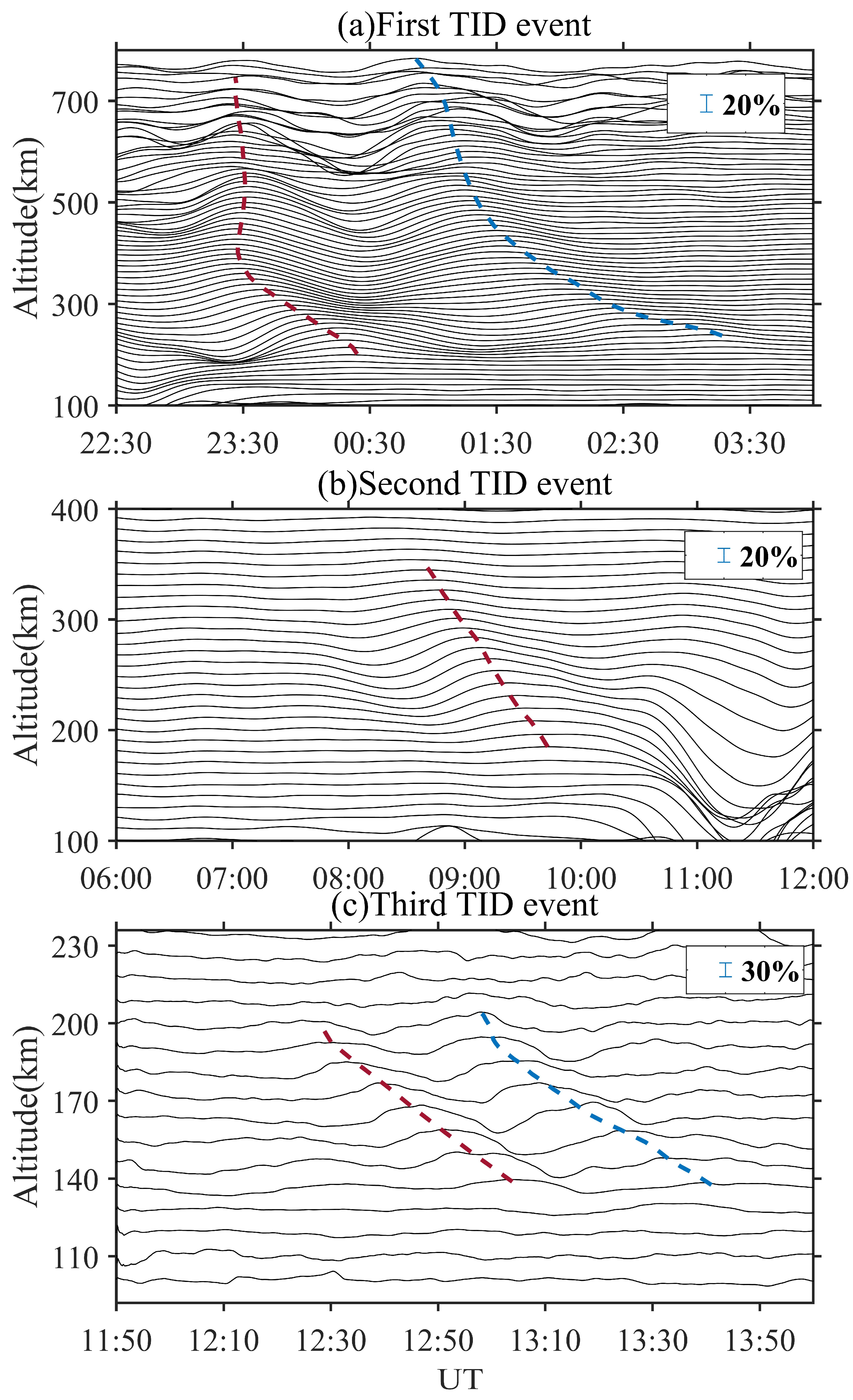
• The two LSTID events exhibit similar yet distinct vertical propagation characteristics. Both events were identified with a dominant period of ~110–155 min and downward vertical phase velocities ranging from 22 m/s to 60 m/s. Their amplitudes continuously increase with increasing altitude and then gradually decrease after reaching their peak at 200–250 km. Additionally, a phase anomaly in the vertical direction of this TID was observed, a phenomenon different from the AGW theory. The first phase of the first LSTID event shows a characteristic with a more vertical phase than the second phase front in the 350–510 km altitude range. This anomaly is likely attributed to the combined effect of sunrise and pre-sunrise uplift. These drastic changes in electron density after sunrise caused a TID-like phase reversal in the filtered phase.
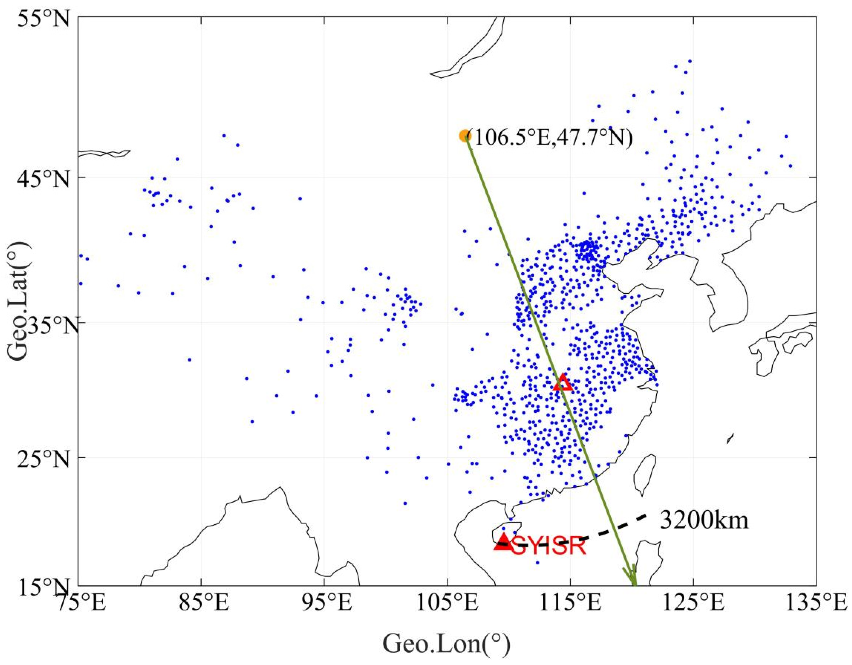
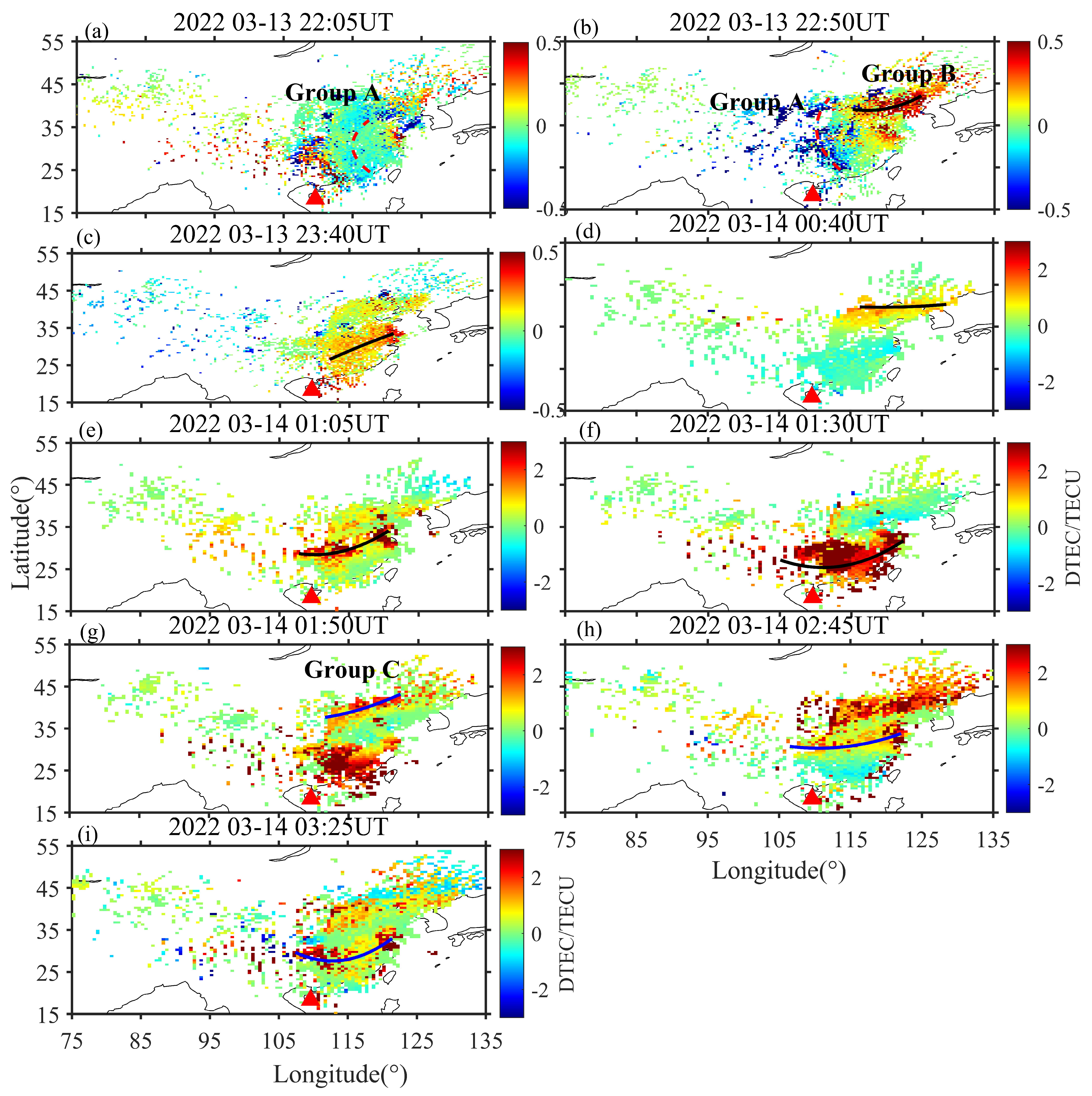
• The different propagation features of the two LSTIDs suggest different sources. The first LSTID event was observed with a relative amplitude of 18–25% at altitudes ranging from 170 km to 700 km. The combined observation of the GNSS network and SYISR showed that the first LSTID originated from the high latitudes of the Asian sector, propagated across East Asia, and then reached Sanya. A smaller estimated elevation angle (~3°–4°) supports the long-distance propagation of the first LSTID. On the other hand, the second LSTID, not detected by GNSS in mainland China and Japan, displayed a smaller amplitude (~17–20%) and lower propagation altitude (150–360 km). The larger estimated elevation angle (~17°) implies that the second LSTID was likely triggered by a local source.
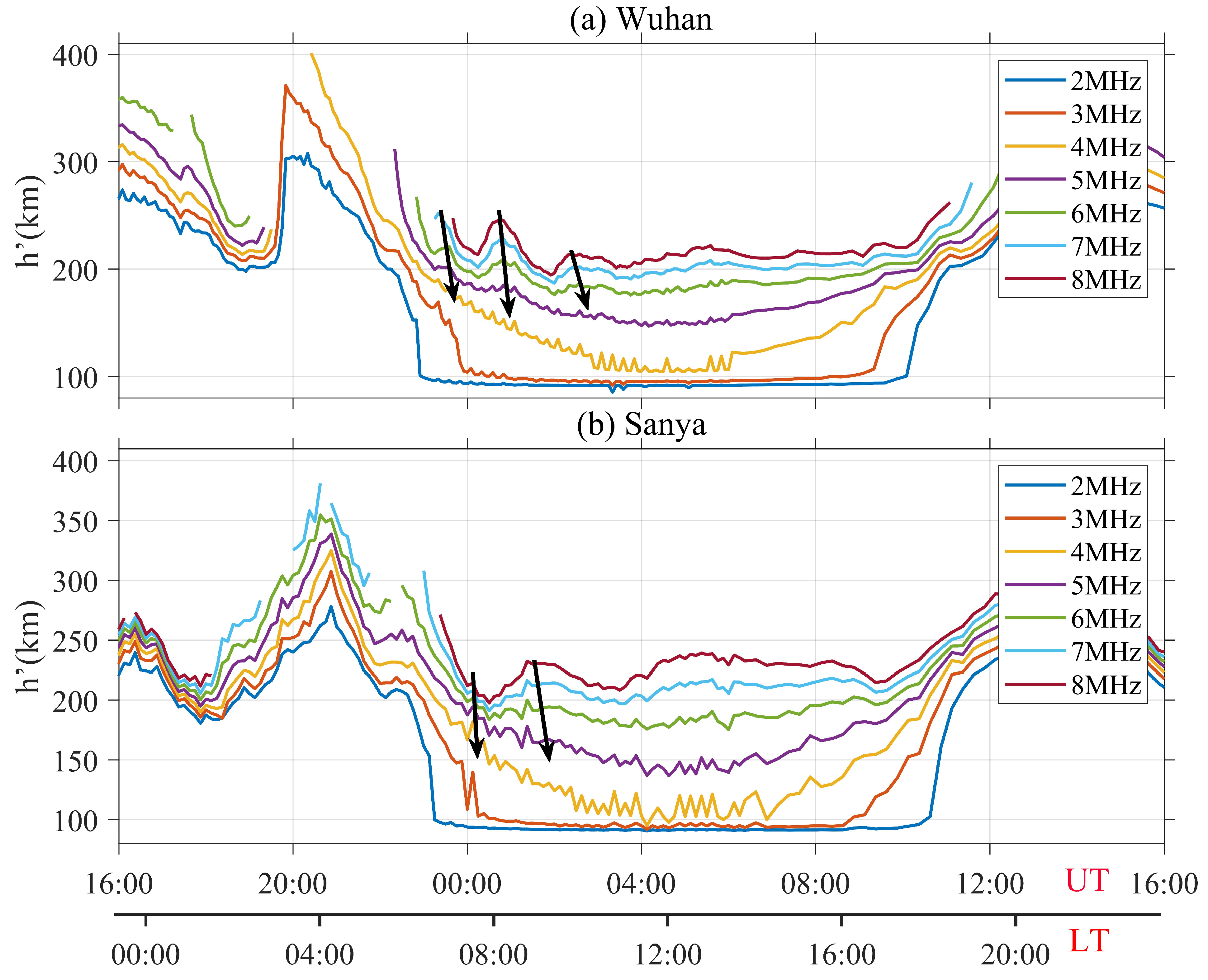
• The periodic MSTID event may be associated with lower atmospheric AGWs. This MSTID event occurred in the lower ionosphere (130–210 km) above Es. Although a notable maximum amplitude of ~29–36% was observed at ~130 km altitude, this TID event dissipated rapidly during its upward propagation at a rate of approximately −1.11%/km.

References

1. Hajkowicz, L.A. Auroral electrojet effect on the global occurrence pattern of large-scale traveling ionospheric disturbances. Planet. Space Sci. 1991, 39, 1189–1196. [Google Scholar] [CrossRef]
2. Ding, F.; Wan, W.; Liu, L.; Afraimovich, E.L.; Voeykov, S.V.; Perevalova, N.P. A statistical study of large-scale traveling ionospheric disturbances observed by GPS TEC during major magnetic storms over the years 2003–2005. J. Geophys. Res. Space Phys. 2008, 113, e2008ja013037. [Google Scholar] [CrossRef]
3. Liu, J.; Zhang, D.H.; Coster, A.J.; Zhang, S.R.; Ma, G.Y.; Hao, Y.Q.; Xiao, Z. A case study of the large-scale traveling ionospheric disturbances in the eastern Asian sector during the 2015 St. Patrick’s Day geomagnetic storm. Ann. Geophys. 2019, 37, 673–687. [Google Scholar] [CrossRef]
4. Unnikrishnan, K.; Saito, A.; Otsuka, Y.; Yamamoto, M.; Fukao, S. Transition region of TEC enhancement phenomena during geomagnetically disturbed periods at mid-latitudes. Ann. Geophys. 2005, 23, 3439–3450. [Google Scholar] [CrossRef]
5. Yeh, K.C.; Liu, C.H.; Youakim, M.Y. Attenuation of internal gravity-waves in model atmospheres. Ann. Geophys. 1975, 31, 321–328. [Google Scholar]
6. Tsugawa, T.; Saito, A.; Otsuka, Y. A statistical study of large-scale traveling ionospheric disturbances using the GPS network in Japan. J. Geophys. Res. Space Phys. 2004, 109, e2003ja010302. [Google Scholar] [CrossRef]
7. Ding, F.; Wan, W.; Ning, B.; Zhao, B.; Li, Q.; Zhang, R.; Xiong, B.; Song, Q. Two-dimensional imaging of large-scale traveling ionospheric disturbances over China based on GPS data. J. Geophys. Res. Space Phys. 2012, 117, e2012ja017546. [Google Scholar] [CrossRef]
8. Liu, C.H.; Yeh, K.C. Effect of ion drag on propagation of acoustic-gravity waves in the atmosphericFregion. J. Geophys. Res. 1969, 74, 2248–2255. [Google Scholar] [CrossRef]
9. Song, Q.; Ding, F.; Wan, W.; Ning, B.; Zhao, B. Monitoring traveling ionospheric disturbances using the GPS network around China during the geomagnetic storm on 28 May 2011. Sci. China Earth Sci. 2013, 56, 718–726. [Google Scholar] [CrossRef]
10. Maeda, S.; Handa, S. Transmission of large-scale tids in the ionospheric f2-region. J. Atmos. Terr. Phys. 1980, 42, 853–859. [Google Scholar] [CrossRef]
11. Song, Q.; Ding, F.; Wan, W.; Ning, B.; Liu, L. Global propagation features of large-scale traveling ionospheric disturbances during the magnetic storm of 7~10 November 2004. Ann. Geophys. 2012, 30, 683–694. [Google Scholar] [CrossRef]
12. Wang, M.; Ding, F.; Wan, W.; Ning, B.; Zhao, B. Monitoring global traveling ionospheric disturbances using the worldwide GPS network during the October 2003 storms. Earth Planets Space 2007, 59, 407–419. [Google Scholar] [CrossRef]
13. Ding, F.; Wan, W.; Li, Q.; Zhang, R.; Song, Q.; Ning, B.; Liu, L.; Zhao, B.; Xiong, B. Comparative climatological study of large-scale traveling ionospheric disturbances over North America and China in 2011–2012. J. Geophys. Res.-Space Phys. 2014, 119, 519–529. [Google Scholar] [CrossRef]
14. Aa, E.; Zhang, S.R.; Erickson, P.J.; Coster, A.J.; Goncharenko, L.P.; Varney, R.H.; Eastes, R. Salient Midlatitude Ionosphere-Thermosphere Disturbances Associated With SAPS During a Minor but Geo-Effective Storm at Deep Solar Minimum. J. Geophys. Res. Space Phys. 2021, 126, e2021ja029509. [Google Scholar] [CrossRef]
15. Jonah, O.F.; Coster, A.; Zhang, S.; Goncharenko, L.; Erickson, P.J.; de Paula, E.R.; Kherani, E.A. TID Observations and Source Analysis During the 2017 Memorial Day Weekend Geomagnetic Storm Over North America. J. Geophys. Res.-Space Phys. 2018, 123, 8749–8765. [Google Scholar] [CrossRef]
16. Chen, G.; Ding, F.; Wan, W.; Hu, L.; Zhao, X.; Li, J. Structures of Multiple Large-Scale Traveling Ionospheric Disturbances Observed by Dense Global Navigation Satellite System Networks in China. J. Geophys. Res. Space Phys. 2020, 125, e2019ja027032. [Google Scholar] [CrossRef]
17. Ding, F.; Wan, W.; Ning, B.; Zhao, B.; Li, Q.; Wang, Y.; Hu, L.; Zhang, R.; Xiong, B. Observations of poleward-propagating large-scale traveling ionospheric disturbances in southern China. Ann. Geophys. 2013, 31, 377–385. [Google Scholar] [CrossRef]
18. Jacobson, A.R.; Carlos, R.C. A study of apparent ionospheric motions associated with multiple traveling ionospheric disturbances. J. Atmos. Terr. Phys. 1991, 53, 53–62. [Google Scholar] [CrossRef]
19. Chimonas, G. Equatorial electrojet as a source of long period travelling ionospheric disturbances. Up. Atmos. Motion 1974, 18, 698–706. [Google Scholar] [CrossRef]
20. Vadas, S.L.; Liu, H.l. Generation of large-scale gravity waves and neutral winds in the thermosphere from the dissipation of convectively generated gravity waves. J. Geophys. Res. Space Phys. 2009, 114, e2009ja014108. [Google Scholar] [CrossRef]
21. Borchevkina, O.P.; Karpov, I.V.; Karpov, A.I. Observations of Acoustic Gravity Waves during the Solar Eclipse of March 20, 2015 in Kaliningrad. Russ. J. Phys. Chem. B 2017, 11, 1024–1027. [Google Scholar] [CrossRef]
22. Thome, G.D. Incoherent scatter observations of traveling ionospheric disturbances. J. Geophys. Res. 1964, 69, 4047–4049. [Google Scholar] [CrossRef]
23. Harper, R.M.; Woodman, R.F. Preliminary multiheight radar observations of waves and winds in mesosphere over jicamarca. J. Atmos. Terr. Phys. 1977, 39, 959–963. [Google Scholar] [CrossRef]
24. Sterling, D.L.; Hooke, W.H.; Cohen, R. Traveling ionospheric disturbances observed at the magnetic equator. J. Geophys. Res. 1971, 76, 3777–3782. [Google Scholar] [CrossRef]
25. Bertin, F.; Kofman, W.; Lejeune, G. Observations of gravity-waves in the auroral-zone. Radio Sci. 1983, 18, 1059–1065. [Google Scholar] [CrossRef]
26. Vlasov, A.; Kauristie, K.; van de Kamp, M.; Luntama, J.P.; Pogoreltsev, A. A study of Traveling Ionospheric Disturbances and Atmospheric Gravity Waves using EISCAT Svalbard Radar IPY-data. Ann. Geophys. 2011, 29, 2101–2116. [Google Scholar] [CrossRef]
27. Oliver, W.L.; Otsuka, Y.; Sato, M.; Takami, T.; Fukao, S. A climatology of F region gravity wave propagation over the middle and upper atmosphere radar. J. Geophys. Res. Space Phys. 1997, 102, 14499–14512. [Google Scholar] [CrossRef]
28. Thome, G. Long-period waves generated in the polar ionosphere during the onset of magnetic storms. J. Geophys. Res. 1968, 73, 6319–6336. [Google Scholar] [CrossRef]
29. Ma, S.Y.; Schlegel, K.; Xu, J.S. Case studies of the propagation characteristics of auroral TIDS with EISCAT CP2 data using maximum entropy cross-spectral analysis. Ann. Geophys.-Atmos. Hydrospheres Space Sci. 1998, 16, 161–167. [Google Scholar] [CrossRef]
30. van de Kamp, M.; Pokhotelov, D.; Kauristie, K. TID characterised using joint effort of incoherent scatter radar and GPS. Ann. Geophys. 2014, 32, 1511–1532. [Google Scholar] [CrossRef]
31. Djuth, F.T.; Zhang, L.D.; Livneh, D.J.; Seker, I.; Smith, S.M.; Sulzer, M.P.; Mathews, J.D.; Walterscheid, R.L. Arecibo’s thermospheric gravity waves and the case for an ocean source. J. Geophys. Res. Space Phys. 2010, 115, e2009ja014799. [Google Scholar] [CrossRef]
32. Yue, X.; Wan, W.; Ning, B.; Jin, L.; Ding, F.; Zhao, B.; Zeng, L.; Ke, C.; Deng, X.; Wang, J.; et al. Development of the Sanya Incoherent Scatter Radar and Preliminary Results. J. Geophys. Res. Space Phys. 2022, 127, e2022ja030451. [Google Scholar] [CrossRef]
33. Damtie, B.; Nygrén, T.; Lehtinen, M.S.; Huuskonen, A. High resolution observations of sporadic-E layers within the polar cap ionosphere using a new incoherent scatter radar experiment. Ann. Geophys. 2002, 20, 1429–1438. [Google Scholar] [CrossRef]
34. Damtie, B.; Lehtinen, M.S.; Nygrén, T. Decoding of Barker-coded incoherent scatter measurements by means of mathematical inversion. Ann. Geophys. 2004, 22, 3–13. [Google Scholar] [CrossRef]
35. Mathews, J.D. Incoherent-scatter radar probing of the 60-100-km atmosphere and ionosphere. IEEE Trans. Geosci. Remote Sens. 1986, 24, 765–776. [Google Scholar] [CrossRef]
36. Yue, X.; Cai, Y.; Wang, J.; Lei, J.; Wang, Z.; Wang, Y.; Li, M.; Zhang, N.; Ding, F.; Ning, B. Ionospheric Pre-Sunrise Uplift: Comparison of Sanya Incoherent Scatter Radar Observations and Numerical Simulations. J. Geophys. Res. Space Phys. 2023, 128, e2022ja031119. [Google Scholar] [CrossRef]
37. Zhang, H.P.; Zhu, W.Y.; Peng, J.H.; Huang, C. Analysis of the ionosphere wave-motion with GPS. Chin. Sci. Bull. 2005, 50, 1373–1381. [Google Scholar] [CrossRef]
38. Lee, M.C.; Pradipta, R.; Burke, W.J.; Labno, A.; Burton, L.M.; Cohen, J.A.; Dorfman, S.E.; Coster, A.J.; Sulzer, M.P.; Kuo, S.P. Did Tsunami-Launched Gravity Waves Trigger Ionospheric Turbulence over Arecibo? J. Geophys. Res. Space Phys. 2008, 113, e2007ja012615. [Google Scholar] [CrossRef]
39. Park, J.; Min, K.W.; Kim, V.P.; Kil, H.; Kim, H.J.; Lee, J.J.; Lee, E.; Kim, S.J.; Lee, D.Y.; Hairston, M. Statistical description of low-latitude plasma blobs as observed by DMSP F15 and KOMPSAT-1. Adv. Space Res. 2008, 41, 650–654. [Google Scholar] [CrossRef]
40. Welling, D.T.; André, M.; Dandouras, I.; Delcourt, D.; Fazakerley, A.; Fontaine, D.; Foster, J.; Ilie, R.; Kistler, L.; Lee, J.H.; et al. The Earth: Plasma Sources, Losses, and Transport Processes. Space Sci. Rev. 2015, 192, 145–208. [Google Scholar] [CrossRef]
41. Gong, Y.; Zhou, Q.; Zhang, S.; Aponte, N.; Sulzer, M.; Gonzalez, S. Midnight ionosphere collapse at Arecibo and its relationship to the neutral wind, electric field, and ambipolar diffusion. J. Geophys. Res. Space Phys. 2012, 117, e2012ja017530. [Google Scholar] [CrossRef]
42. Fukao, S.; Yamamoto, Y.; Oliver, W.L.; Takami, T.; Yamanaka, M.D.; Yamamoto, M.; Nakamura, T.; Tsuda, T. Middle and upper-atmosphere radar observations of ionospheric horizontal gradients produced by gravity-waves. J. Geophys. Res.-Space Phys. 1993, 98, 9443–9451. [Google Scholar] [CrossRef]
43. Zhang, S.R.; Oliver, W.L.; Fukao, S.; Otsuka, Y. A study of the forenoon ionospheric F2 layer behavior over the middle and upper atmospheric radar. J. Geophys. Res. Space Phys. 2000, 105, 15823–15833. [Google Scholar] [CrossRef]
44. Le, H.; Liu, L.; Chen, B.; Lei, J.; Yue, X.; Wan, W. Modeling the responses of the middle latitude ionosphere to solar flares. J. Atmos. Sol.-Terr. Phys. 2007, 69, 1587–1598. [Google Scholar] [CrossRef]
45. Le, H.; Liu, L.; Yue, X.; Wan, W. The ionospheric behavior in conjugate hemispheres during the 3 October 2005 solar eclipse. Ann. Geophys. 2009, 27, 179–184. [Google Scholar] [CrossRef]
46. Nicolls, M.J.; Kelley, M.C.; Coster, A.J.; González, S.A.; Makela, J.J. Imaging the structure of a large-scale TID using ISR and TEC data. Geophys. Res. Lett. 2004, 31, e2004gl019797. [Google Scholar] [CrossRef]
47. Negale, M.R.; Taylor, M.J.; Nicolls, M.J.; Vadas, S.L.; Nielsen, K.; Heinselman, C.J. Seasonal Propagation Characteristics of MSTIDs Observed at High Latitudes Over Central Alaska Using the Poker Flat Incoherent Scatter Radar. J. Geophys. Res. Space Phys. 2018, 123, 5717–5737. [Google Scholar] [CrossRef]
48. Bossert, K.; Paxton, L.J.; Matsuo, T.; Goncharenko, L.; Kumari, K.; Conde, M. Large-Scale Traveling Atmospheric and Ionospheric Disturbances Observed in GUVI With Multi-Instrument Validations. Geophys. Res. Lett. 2022, 49, e2022gl099901. [Google Scholar] [CrossRef]
49. Nicolls, M.J.; Vadas, S.L.; Aponte, N.; Sulzer, M.P. Horizontal parameters of daytime thermospheric gravity waves and E region neutral winds over Puerto Rico. J. Geophys. Res. Space Phys. 2014, 119, 575–600. [Google Scholar] [CrossRef]
50. Vargas, F. Traveling Ionosphere Disturbance Signatures on Ground-Based Observations of the O(1D) Nightglow Inferred From 1-D Modeling. J. Geophys. Res. Space Phys. 2019, 124, 9348–9363. [Google Scholar] [CrossRef]
51. Vadas, S.L. Horizontal and vertical propagation and dissipation of gravity waves in the thermosphere from lower atmospheric and thermospheric sources. J. Geophys. Res. Space Phys. 2007, 112, e2006ja011845. [Google Scholar] [CrossRef]
52. Hines, C.O. Gravity-waves in atmosphere. Nature 1972, 239, 73. [Google Scholar] [CrossRef]
53. Lanchester, B.S.; Nygren, T.; Jarvis, M.J.; Edwards, R. Gravity-wave parameters measured with eiscat and dynasonde. Ann. Geophys.-Atmos. Hydrospheres Space Sci. 1993, 11, 925–936. [Google Scholar]
54. Morgan, M.G. Daytime traveling ionospheric disturbances observed at L ≈ 4.5 in western Quebec with rapid-run ionosondes. Radio Sci. 1990, 25, 73–83. [Google Scholar] [CrossRef]
55. Bristow, W.A.; Greenwald, R.A.; Samson, J.C. Identification of high-latitude acoustic gravity wave sources using the Goose Bay HF Radar. J. Geophys. Res. Space Phys. 1994, 99, 319–331. [Google Scholar] [CrossRef]
56. Gardner, L.C.; Schunk, R.W. Large-scale gravity wave characteristics simulated with a high-resolution global thermosphere-ionosphere model. J. Geophys. Res. Space Phys. 2011, 116, e2010ja015629. [Google Scholar] [CrossRef]
57. Yakovets, A.F.; Vodyannikov, V.V.; Gordienko, G.I.; Litvinov, Y.G. Height profiles of the amplitudes of large-scale traveling ionospheric disturbances. Geomagn. Aeron. 2013, 53, 655–662. [Google Scholar] [CrossRef]
58. Huang, C.S.; Sofko, G.J.; Kelley, M.C. Numerical simulations of midlatitude ionospheric perturbations produced by gravity waves. J. Geophys. Res. Space Phys. 1998, 103, 6977–6989. [Google Scholar] [CrossRef]
59. Morgan, M.G.; Ballard, K.A. The height dependence of wave-normal depression and disturbance amplitude in TID’s. J. Geophys. Res. Space Phys. 1978, 83, 5741–5744. [Google Scholar] [CrossRef]
60. Djuth, F.T.; Sulzer, M.P.; Elder, J.H.; Wickwar, V.B. High-resolution studies of atmosphere-ionosphere coupling at Arecibo Observatory, Puerto Rico. Radio Sci. 1997, 32, 2321–2344. [Google Scholar] [CrossRef]
61. Vadas, S.L.; Fritts, D.C. Influence of solar variability on gravity wave structure and dissipation in the thermosphere from tropospheric convection. J. Geophys. Res. Space Phys. 2006, 111, e2005ja011510. [Google Scholar] [CrossRef]
62. Kirchengast, G. Elucidation of the physics of the gravity wave-TID relationship with the aid of theoretical simulations. J. Geophys. Res. Space Phys. 1996, 101, 13353–13368. [Google Scholar] [CrossRef]
63. Hines, C.O. Some consequences of gravity-wave critical layers in upper atmosphere. J. Atmos. Terr. Phys. 1968, 30, 837–843. [Google Scholar] [CrossRef]
64. Gossard, E.; Munk, W. On gravity waves in the atmosphere. J. Meteorol. 1954, 11, 259–269. [Google Scholar] [CrossRef]
65. Kirchengast, G.; Hocke, K.; Schlegel, K. Gravity waves determined by modeling of traveling ionospheric disturbances in incoherent-scatter radar measurements. Radio Sci. 1995, 30, 1551–1567. [Google Scholar] [CrossRef]
66. Hocke, K.; Schlegel, K. A review of atmospheric gravity waves and travelling ionospheric disturbances: 1982-1995. Ann. Geophys. 1996, 14, 917–940. [Google Scholar] [CrossRef]
67. Vadas, S.L.; Nicolls, M.J. Temporal evolution of neutral, thermospheric winds and plasma response using PFISR measurements of gravity waves. J. Atmos. Sol.-Terr. Phys. 2009, 71, 744–770. [Google Scholar] [CrossRef]
68. Georges, T.M. HF Doppler studies of traveling ionospheric disturbances. J. Atmos. Terr. Phys. 1968, 30, 735–746. [Google Scholar] [CrossRef]
69. Hearn, A.L.; Yeh, K.C. Medium scale TID’s and their associated internal gravity waves as seen through height-dependent electron density power spectra. J. Geophys. Res. 1977, 82, 4983–4990. [Google Scholar] [CrossRef]
70. Liu, Y.; Zhou, C.; Tang, Q.; Kong, J.; Gu, X.; Ni, B.; Yao, Y.; Zhao, Z. Evidence of Mid- and Low-Latitude Nighttime Ionospheric E-F Coupling: Coordinated Observations of Sporadic E Layers, F-Region Field-Aligned Irregularities, and Medium-Scale Traveling Ionospheric Disturbances. IEEE Trans. Geosci. Remote Sens. 2019, 57, 7547–7557. [Google Scholar] [CrossRef]
71. Perkins, F. SpreadFand ionospheric currents. J. Geophys. Res. 1973, 78, 218–226. [Google Scholar] [CrossRef]
72. Figueiredo, C.A.O.B.; Takahashi, H.; Wrasse, C.M.; Otsuka, Y.; Shiokawa, K.; Barros, D. Investigation of Nighttime MSTIDS Observed by Optical Thermosphere Imagers at Low Latitudes: Morphology, Propagation Direction, and Wind Filtering. J. Geophys. Res.-Space Phys. 2018, 123, 7843–7857. [Google Scholar] [CrossRef]
Figure 1. Geomagnetic conditions for 13–18 March 2022: (a) the By and Bz components of the interplanetary magnetic field observed by ACE, (b) 3 hr Kp index, and (c) SYM-H. The blue shaded area indicates the main phase of the magnetic storm, and the black dashed line indicates the local sunrise time at ground level in Sanya.
Remotesensing 16 03126 g001
Figure 2. The geographical location of the SYISR station (red triangle) and ground-based global navigation satellite system (GNSS) receivers in China (blue dots). The green line is the horizontal distance axis set to calculate the DTEC keogram across China. The dashed line represents an arc with a radius of 3200 km from the origin of the coordinate axis (yellow dot). The distance of 3200 km approximately corresponds to the distance from the origin to the SYISR location. The red hollow triangle indicates the location of the ionosonde at the Wuhan station.
Remotesensing 16 03126 g002
Figure 3. SYISR observations on 13–14 March 2022. (a) Raw electron density. (b h m F 2  before and after 14 March 2022. The red inverted triangle indicates when the first TID appeared. The black rectangle is an enlarged view of  h m F 2  on 14 March near the appearance of the LSTID event. (c) Bandpass-filtered relative electron density perturbation ( δ N e / N e ). The sunrise and sunset are marked as black dashed lines. The white arrow indicates the propagation direction of two LSTID events.
Remotesensing 16 03126 g003
Figure 4. A time series profile of relative electron density perturbations at different altitudes for the three TID events. (a) The first TID event. The altitude sampling interval is 10 km. The blue and red dashed lines indicate the phase fronts. (b) The second TID event. The altitude sampling interval is 10 km. (c) The third TID event. The altitude sampling interval is 9 km. The mark at the top right corner is the relative amplitude scale.
Remotesensing 16 03126 g004
Figure 5. (ai) Two-dimensional differential total electron content (DTEC) maps from 13 March 22:05 UT to 14 March 03:25 UT. The colors represent the deviation in the TEC in units of TECU. The solid lines in black and dark blue correspond to the TID phase lines fitted by the peak positions of TEC perturbations. The red dashed line indicates the TID phase front induced by ST. The red triangle represents the location of the SYISR.
Remotesensing 16 03126 g005
Figure 6. Variations in TEC as a function of the UT and distance across the slice shown in Figure 1. The solid and dashed arrows indicate the location of the peaks and valleys of the TID, respectively.
Remotesensing 16 03126 g006
Figure 7. Temporal variations in virtual height, at detection frequencies ranging from 2 to 8 MHz, with a step of 1 MHz, recorded by the ionosonde chain in China on 13–14 March 2022. Frequencies are shown on each curve. The frequencies and virtual heights were read from the F-layer trace in the ionograms recorded by ionosondes in (a) Wuhan (30.5°N) and (b) Sanya (18.3°N). The time resolution is 7.5 min. The black arrow lines in each plot connect the peaks of variation at different frequencies.
Remotesensing 16 03126 g007
Disclaimer/Publisher’s Note: The statements, opinions and data contained in all publications are solely those of the individual author(s) and contributor(s) and not of MDPI and/or the editor(s). MDPI and/or the editor(s) disclaim responsibility for any injury to people or property resulting from any ideas, methods, instructions or products referred to in the content.