Multi-Target Pairing Method Based on PM-ESPRIT-like DOA Estimation for T/R-R HFSWR

Abstract

The transmit/receive-receive (T/R-R) synergetic High Frequency Surface Wave Radar (HFSWR) has increasingly attracted attention due to its high localization accuracy, but multi-target pairing needs to be performed before localization in multi-target scenarios. However, existing multi-target parameter matching methods have primarily focused on track association, which falls under the category of information-level fusion techniques, with few methods based on detected points. In this paper, we propose a multi-target pairing method with high computational efficiency based on angle information for T/R-R synergetic HFSWR. To be more specific, a dual-receiving array signal model under long baseline condition is firstly constructed. Then, the amplitude and phase differences of the same target reaching two subarrays are calculated to establish the cross-correlation matrix. Subsequently, in order to extract the rotation factor matrices containing pairing information and improve angle estimation performance, we utilize the conjugate symmetry properties of the uniform linear array (ULA) manifold matrix for generalized virtual aperture extension. Ultimately, azimuths estimation and multi-target pairing are accomplished by combining the propagator method (PM) and the ESPRIT algorithm. The proposed method relies solely on angle information for multi-target pairing and leverages the rotational invariance property of Vandermonde matrices to avoid peak searching or iterations, making it computationally efficient. Furthermore, the proposed method maintains superb performance regardless of whether the spatial angles are widely separated or very close. Simulation results validate the effectiveness of the proposed method.

1. Introduction

HFSWR functions in a shortwave band of 3 MHz to 30 MHz. Unlike conventional microwave radars, which are limited to detecting targets within the line of sight, the vertically polarized electromagnetic waves in this band can propagate beyond the Earth’s curvature by diffracting along the sea surface with low loss. Therefore, HFSWR systems are typically used for over-the-horizon detection of maritime and low-altitude targets, enabling the detection and tracking of targets up to 500 kilometers away and also facilitating the remote sensing of ocean parameters [1,2,3,4,5]. Notable examples of such systems include the Ocean Surface Current Radar (OSCR) system [6] in Britain and the SWR-503 [7] system in Canada. Due to its large occupied area and difficulty of deployment, compact HFSWR systems have been developed, such as the array antenna-based WERA-S system [8] in Germany, the cross-loop antenna-based SeaSonde system [9] in the United States, etc.

A traditional HFSWR system is composed of a transmitting antenna and a receiving antenna array, as shown in Figure 1a. Commonly, HFSWR operates in a monostatic transmit/receive (T/R) mode, which means that the system places the transmitting antenna and the receiver at the same site near the coastline. The transmitting antenna employs a wideband antenna to radiate radar waveform signals, covering the detection area. Simultaneously, the receiving antenna array captures the echoes reflected by targets, facilitating target detection and tracking. To achieve the required azimuth accuracy and directional gain, the receiving antenna array typically comprises array elements spanning several hundred meters in total length [10,11].

As the demand for modern maritime surveillance intensifies, multistatic HFSWR systems have attracted widespread attention [12]. The simplest form of multistatic HFSWR systems is the T/R-R synergetic HFSWR configuration. As illustrated in Figure 1b, the T/R-R synergetic HFSWR setup consists of a monostatic radar paired with an extra receiving array. This configuration includes a single transmitting antenna alongside two receiving arrays. Among these, one receiving array is situated near the transmitting antenna while the other is placed at a remote location. This arrangement offers flexibility and concealment for the receivers [13,14,15]. Furthermore, with the increase in the number of receivers, the coverage area is expanded, allowing targets to be independently detected and tracked within the overlapping detection zones of the two radars. Additionally, the overall performance of the radar system can be enhanced through the use of signal-level and information-level fusion technologies [16,17].

So far, there has been limited development of T/R-R synergetic HFSWR. Existing research on T/R-R synergetic radar systems primarily focuses on theoretical and simulation analysis [5,14,18,19]. A two-dimensional imaging algorithm is introduced in [20] for rotating targets using a T/R-R bistatic radar system. Sun et al. explore a vessel tracking algorithm employing a T-R bistatic compact HFSWR [21]. A T/R-R synergetic HFSWR approach to enhance target detection and flight mode recognition is proposed [18]. Sun et al. suggest a method to estimate ship speed and heading from Doppler echoes using a T/R-R composite compact HFSWR [22]. In addition, these papers [23,24,25,26] discuss the beam-space methods of bistatic systems, and an algorithm for deriving directional ocean wave spectra by effectively utilizing synthetic bistatic HFSWR data is described in [19].

In recent years, a significant number of localization methods through direction estimation have been investigated in bistatic radar systems [27,28]. However, research on multi-target pairing is scarce, with the majority of studies on multi-target pairing for T/R-R radars focusing on track-to-track association [29,30,31,32,33], which is part of information-level fusion technology, while fewer methods directly achieve target pairing from detected points. The only retrievable method using detected points is the one proposed in our earlier work [34], which is based on angle estimation information for multi-target pairing. But its performance is significantly affected by the spatial position of the targets, especially when dealing with targets with small angular intervals. Additionally, research on multi-target pairing in array signal processing also appears in the literature related to two-dimensional direction-of-arrival (2D-DOA) estimation using L-shaped arrays, where these methods can perform multi-target two-dimensional parameter pairing based on estimated 2D-DOA information [35,36,37,38]. Nevertheless, these 2-D DOA methods capable of multi-target pairing on L-shaped arrays are not applicable to T/R-R synergetic radar systems, as the echo signals arriving at the two receiving arrays are inconsistent when there is a long baseline separation between the two receiving arrays.

In this paper, we propose a method that combines the Propagator Method (PM) with the ESPRIT algorithm, utilizing only the estimated angle information to achieve multi-target pairing in T/R-R synergetic radar systems. Specifically, based on the spherical wave equation, the differences in amplitude and phase of target echoes arriving at the two subarrays are calculated, which are then utilized to construct a cross-correlation matrix for long baseline array signals. Following this, the conjugate symmetry of ULAs manifold matrices is exploited to effectively extend the array aperture. A large generalized received data matrix is subsequently built, and its propagator matrix is obtained using the Propagator Method (PM). Finally, by leveraging the rotation-invariant property of the array manifold matrix constructed from the propagator matrix, the ESPRIT algorithm is used to estimate the azimuths of the two subarrays and achieve multi-target pairing. Simulation results demonstrate that the proposed method achieves better angle estimation accuracy and multi-target pairing performance compared to the MPTV [34] method.

The proposed method is characterized by several features and advantages:

(1)

The proposed method belongs to the class of DOA estimation algorithms and relies solely on angle information for multi-target pairing.

(2)

Unlike track association methods, the proposed method eliminates the need for multiframe association operations and complex mathematical computations. Moreover, the proposed method does not require iterative operations or spectral peak searching, making it computationally efficient.

(3)

If the two subarrays are considered as a single non-uniform linear array for angle estimation and multi-target pairing, the long baseline can lead to grating lobes and angle ambiguity. The proposed method can avoid these issues.

(4)

By employing the generalized virtual array aperture extension, we construct a large generalized received data matrix, which enables the proposed method to maintain robust angle estimation and multi-target pairing performance under small angular interval target conditions.

This paper is structured as follows: In Section 2, the dual receiving arrays model of a receiving system is formulated. The multi-target pairing method utilizing the generalized virtual array aperture extension technique is proposed in Section 3. Section 4 validates the effectiveness of the proposed method by presenting simulation results and providing a thorough analysis. The conclusions are drawn in Section 5.

Notations: The notational conventions established within this paper are as follows: capital boldface letters, lower-case letters, and nonboldface letters indicate matrices, column vectors, and scalars, respectively. ${\left(·\right)}^H$, ${\left(·\right)}^T$, ${\left(·\right)}^{*}$, ${\left(·\right)}^{†}$, and ${\left(·\right)}^{-1}$ denote Hermitian transpose, transpose, conjugate, persudo-inverse, and inverse, respectively. The notations $diag\left\{·\right\}$ and $phase\left\{·\right\}$ stand for the diagonalization on a vector and phase angle operator for complex number. While ${\mathbf{O}}_{m\times n}$, ${\mathbf{I}}_M$, ${\mathbf{J}}_M$ and ⊗ denote respectively an $m\times n$ zero matrix, an $M\times M$ identity matrix, an $M\times M$ exchange matrix with ones on its anti-diagonal and zeros elsewhere, and Kronecker product. Additionally, $E\left\{·\right\}$ and ${\delta }_{m,t}$ represent the expectation operation and Kronecker delta.

2. Signal Model

When using the HFSWR radar system to monitor maritime and low-altitude targets, the accuracy of azimuth angle calculation only concerns the receiving array and is unrelated to the transmitting array. Therefore, only the receiving array needs to be considered when modeling. The dual receiving arrays model of the T/R-R synergetic radar system is shown in Figure 2. Two independent uniform linear arrays $S_1$ and $S_2$ are arranged horizontally on the same baseline to form the T/R-R synergetic radar receiving array system. Each receiving array contains N isotropic sensors with intersensor spacing d. The coordinates of the reference sensors for the two arrays are $S_1\left(x,y\right)$ and $S_2\left(x,y\right)$, respectively, with L representing the baseline length between the two arrays, and $L\gg Nd$.

Assume that K targets are randomly distributed in the space, with $r_{1,k}$ and $r_{2,k}$, $k=1,2,\cdots K$ denoting the distances between the two subarrays and the kth target. The transmitting array emits electromagnetic waves to irradiate the targets, and after reflection, K uncorrelated narrowband far-field signals with wavelength $\lambda$ impinging on the two receiving arrays, respectively. The azimuth of the kth target relative to $S_1$-subarray and $S_2$-subarray are denoted by ${\theta }_k$ and ${\phi }_k$, $k=1,2,\cdots K$, where ${\theta }_k\ne {\theta }_i$, ${\phi }_k\ne {\phi }_i$ for $k\ne i$. It is noteworthy that both ${\theta }_k$ and ${\phi }_k$ refer to the angles between the impinging signal and x-axis.

Let $\mathbf{x}\left(n\right)={\left[x_1\left(n\right),x_2\left(n\right),\cdots ,x_N\left(n\right)\right]}^T$ and $\mathbf{z}\left(n\right)={\left[z_1\left(n\right),z_2\left(n\right),\cdots ,z_N\left(n\right)\right]}^T$ represent the data vectors obtained from the nth snapshot of the $S_1$-subarray and $S_2$-subarray, respectively, which can be expressed as

$$\mathbf{x}\left(n\right)={\mathbf{A}}_x\left(\theta \right){\mathbf{s}}_x\left(n\right)+{\mathbf{n}}_x\left(n\right),$$

(1)

$$\mathbf{z}\left(n\right)={\mathbf{A}}_z\left(\phi \right){\mathbf{s}}_z\left(n\right)+{\mathbf{n}}_z\left(n\right),$$

(2)

respectively, where ${\mathbf{A}}_x\left(\theta \right)$ and ${\mathbf{A}}_z\left(\phi \right)$ denote the array manifold matrices of the two subarrays, which can be written as

$${\mathbf{A}}_x\left(\theta \right)=\left[\mathbf{a}\left({\theta }_1\right)\right.,\cdots ,\mathbf{a}\left({\theta }_k\right),\cdots \left.,\mathbf{a}\left({\theta }_K\right)\right],$$

(3)

$$\mathbf{a}\left({\theta }_k\right)={\left[1,{\xi }_k,{\xi }_k^2,\cdots ,{\xi }_k^{N-1}\right]}^T,k=1,2,\cdots K,$$

(4)

$${\xi }_k=\exp \left(j2\pi d\cos {\theta }_k/\phantom{j2\pi d\cos {\theta }_k\lambda }\lambda \right),$$

(5)

$${\mathbf{A}}_z\left(\phi \right)=\left[\mathbf{a}\left({\phi }_1\right)\right.,\cdots ,\mathbf{a}\left({\phi }_k\right),\cdots \left.,\mathbf{a}\left({\phi }_K\right)\right],$$

(6)

$$\mathbf{a}\left({\phi }_k\right)={\left[1,{\eta }_k,{\eta }_k^2,\cdots ,{\eta }_k^{N-1}\right]}^T,k=1,2,\cdots K,$$

(7)

$${\eta }_k=\exp \left(j2\pi d\cos {\phi }_k/\phantom{j2\pi d\cos {\phi }_k\lambda }\lambda \right).$$

(8)

Let ${\mathbf{s}}_x\left(n\right)$ and ${\mathbf{s}}_z\left(n\right)$ represent the $K\times 1$ signal source vectors of $S_1$-subarray and $S_2$-subarray

$${\mathbf{s}}_x\left(n\right)={\left[s_{x1}\left(n\right),s_{x2}\left(n\right),\cdots ,s_{xK}\left(n\right)\right]}^T,$$

(9)

$${\mathbf{s}}_z\left(n\right)={\left[s_{z1}\left(n\right),s_{z2}\left(n\right),\cdots ,s_{zK}\left(n\right)\right]}^T.$$

(10)

${\mathbf{n}}_x\left(n\right)$ and ${\mathbf{n}}_z\left(n\right)$ denote the additive noise in $S_1$-subarray and $S_2$-subarray, respectively,

$${\mathbf{n}}_x\left(n\right)={\left[n_{x1}\left(n\right),n_{x2}\left(n\right),\cdots ,n_{xN}\left(n\right)\right]}^T,$$

(11)

$${\mathbf{n}}_z\left(n\right)={\left[n_{z1}\left(n\right),n_{z2}\left(n\right),\cdots ,n_{zN}\left(n\right)\right]}^T.$$

(12)

The basic assumptions for the signal model are as follows:

(1)

The K targets are mutually uncorrelated, and the number of targets is less than the number of sensors in the subarray, i.e., $K<N$.

(2)

The additive noises ${\mathbf{n}}_x\left(n\right)$ and ${\mathbf{n}}_z\left(n\right)$ on the two subarrays are both zero-mean, Gaussian white noises with a variance of ${\sigma }^2$ in time and space. The noises are statistically independent from each other, i.e., $E\left\{{\mathbf{n}}_x\left(n\right){\mathbf{n}}_z^H\left(m\right)\right\}={\mathbf{O}}_{N\times N}$, and their covariance matrix is as follows: $E\left\{{\mathbf{n}}_z\left(n\right){\mathbf{n}}_z^H\left(m\right)\right\}=E\left\{{\mathbf{n}}_x\left(n\right){\mathbf{n}}_x^H\left(m\right)\right\}={\sigma }^2{\mathbf{I}}_N{\delta }_{m,t}$, $E\left\{{\mathbf{n}}_z\left(n\right){\mathbf{n}}_z^T\left(m\right)\right\}=E\left\{{\mathbf{n}}_x\left(n\right){\mathbf{n}}_x^T\left(m\right)\right\}={\mathbf{O}}_{N\times N}\forall m,n$.

(3)

To facilitate theoretical performance analysis, the incident signal ${\mathbf{s}}_x\left(n\right)$ at the $S_1$-subarray is modeled as the zero-mean, temporally complex Gaussian random process, and the associated variance is determined by $E\left\{s_{xk}\left(m\right)s_{xk}^{*}\left(n\right)\right\}=p_k{\delta }_{m,n}$ and $E\left\{s_{xk}\left(m\right)s_{xk}\left(n\right)\right\}=0\forall m,n$ for $k=1,2,\cdots K$.

(4)

The incident signals ${\mathbf{s}}_x\left(n\right)$ and ${\mathbf{s}}_z\left(n\right)$ are statistically independent from the additive noise ${\mathbf{n}}_x\left(n\right)$ and ${\mathbf{n}}_z\left(n\right)$ at the two subarrays.

3. Proposed Method

3.1. Construction of Cross-Correlation Matrix Based on Long Baseline Array Signals

To reduce the impact of the noises, a cross-correlation matrix is constructed by using the data $\mathbf{x}\left(n\right)$ and $\mathbf{z}\left(n\right)$ from the two receiving arrays

$$\begin{array}{cc}\hfill {\mathbf{R}}_{x,z}& =E\left\{\mathbf{x}\left(n\right){\mathbf{z}}^H\left(n\right)\right\}\hfill \\ \hfill & ={\mathbf{A}}_x\left(\theta \right)E\left\{{\mathbf{s}}_x\left(n\right){\mathbf{s}}_z^H\left(n\right)\right\}{\mathbf{A}}_z^H\left(\phi \right)+E\left\{{\mathbf{n}}_x\left(n\right){\mathbf{n}}_z^H\left(n\right)\right\}\hfill \\ \hfill & ={\mathbf{A}}_x\left(\theta \right)E\left\{{\mathbf{s}}_x\left(n\right){\mathbf{s}}_z^H\left(n\right)\right\}{\mathbf{A}}_z^H\left(\phi \right).\hfill \end{array}$$

(13)

When performing multi-target pairing in the T/R-R radar system, it is necessary to calculate $E\left\{{\mathbf{s}}_x\left(n\right){\mathbf{s}}_z^H\left(n\right)\right\}$. At this point, the two subarrays should be considered as a single unit, since the baseline length L is much larger than the subarray aperture $D=Nd$, the distance, azimuth angle, phase and amplitude at which the same source arrives at the two subarrays are no longer the same. When considering the two subarrays as a whole, the source no longer satisfies the narrowband far-field plane wave assumption. As illustrated in Figure 3, the diagram distinguishes between the near-field and far-field, and the Rayleigh distance $r=2L^2/\phantom{2L^2\lambda }\lambda$ from the target to the midpoint of the baseline connecting the two subarrays serves as the boundary for this distinction [39].

In the context of T/R-R synergetic HWFSR, when the baseline length extends to the kilometer scale, the targets within the detectable space no longer satisfy the narrowband far-field conditions when considering $S_1$-subarray and $S_2$-subarray as a single entity. For example, when the baseline length is 10 km, the target must be at least 10,000 km away to meet the far-field condition, which is far beyond the detectable range. The sources should be regarded as propagating in the form of spherical waves, indicating that the propagation distances from the target to the two subarrays are unequal and the phases of the sources at $S_1$-subarray and $S_2$-subarray are different. To achieve multi-target pairing under long baseline conditions, it is essential to calculate the amplitude and phase differences of the same source as it arrives at the two subarrays.

However, for an individual subarray, the inter-sensor spacing is relatively small compared to the array aperture, which is on the order of hundreds of meters. The maximum time difference for the echo signals arriving at each sensor is significantly smaller than the signal bandwidth, resulting in negligible variation in the signal envelope across the sensors. Consequently, the complex envelopes of the signals received by each sensor can be considered approximately equal at the same time, thereby satisfying the narrowband far-field conditions. Under near-field conditions, the wave equation for the echo signal is formulated as [40,41]:

$${\displaystyle \frac{1}{r^2}}{\displaystyle \frac{\partial }{\partial r}}\left(r^2{\displaystyle \frac{\partial s}{\partial r}}\right)+{\displaystyle \frac{1}{r^2\sin \beta }}{\displaystyle \frac{\partial }{\partial \beta }}\left(\sin \phi {\displaystyle \frac{\partial s}{\partial r}}\right)+{\displaystyle \frac{1}{r^2{\sin }^2\beta }}{\displaystyle \frac{{\partial }^{2}s}{\partial {\alpha }^2}}={\displaystyle \frac{1}{c^2}}{\displaystyle \frac{{\partial }^{2}s}{\partial n^2}},$$

(14)

where $\alpha$ and $\beta$ represent the azimuth angle and elevation angle of the target relative to the array, respectively, and c denotes the propagation speed of the electromagnetic wave. In an isotropic medium, the source s does not vary with changes in the elevation angle and azimuth angle. Therefore, Equation (14) can be simplified as follows:

$${\displaystyle \frac{1}{r^2}}{\displaystyle \frac{\partial }{\partial r}}\left(r^2{\displaystyle \frac{\partial s}{\partial r}}\right)={\displaystyle \frac{1}{c^2}}{\displaystyle \frac{{\partial }^{2}s}{\partial n^2}},$$

(15)

where s can be denoted as $s\left(r,n\right)$, and the solution to Equation (15) is then given by

$$s(r,n)={\displaystyle \frac{A}{r}}\exp \left[j(wn-{\displaystyle \frac{2\pi }{\lambda }}r)\right],$$

(16)

where $\omega$ represents the angular frequency of the source, A and $A/r$ represent the amplitude of the source and the amplitude of the source at distance r reaching the receiving array, respectively. To be more practical, considering that the radar cross-section (RCS) of the target varies with different angles and that the phase of the signal changes after reflection from the target, the signals received by $S_1$-subarray and $S_2$-subarray can be expressed as

$$s(r_{1,k},n)={\displaystyle \frac{{\mathrm{\Gamma }}_{1,k}}{r_{1,k}}}\exp [j(wn-{\displaystyle \frac{2\pi }{\lambda }}{r}_{1,k})],$$

(17)

$$s(r_{2,k},n)={\displaystyle \frac{{\mathrm{\Gamma }}_{2,k}}{r_{2,k}}}\exp [j(wn-{\displaystyle \frac{2\pi }{\lambda }}{r}_{2,k})],$$

(18)

where ${\mathrm{\Gamma }}_{1,k}$ and ${\mathrm{\Gamma }}_{2,k}$ represent the amplitude of the reflected signal from the kth target with phase changes. ${\mathrm{\Gamma }}_{1,k}$ and ${\mathrm{\Gamma }}_{2,k}$ are defined as complex numbers with phases uniformly distributed between 0 and $2\pi$. Additionally, $r_{1,k}$ and $r_{2,k}$ denote the distances from the kth target to $S_1$-subarray and $S_2$-subarray, repectively,

$$r_{1,k}={\displaystyle \frac{L}{\sin ({\phi }_k-{\theta }_k)}}\sin \left({\phi }_k\right).$$

(19)

$$r_{2,k}={\displaystyle \frac{L}{\sin ({\phi }_k-{\theta }_k)}}\sin \left({\theta }_k\right).$$

(20)

The expressions for the signals received by the two subarrays can be used to define a scaling factor $q_k$, which represents the ratio of the echo signals from the kth target arriving at the two subarrays.

$$q_k={\displaystyle \frac{s(r_{2,k},n)}{s(r_{1,k},n)}}={\varpi }_k{\displaystyle \frac{r_{1,k}}{r_{2,k}}}\exp \left[j{\displaystyle \frac{2\pi }{\lambda }}(r_{1,k}-r_{2,k})\right].$$

(21)

where ${\varpi }_k={\mathrm{\Gamma }}_{2,k}/\phantom{{\mathrm{\Gamma }}_{2,k}{\mathrm{\Gamma }}_{1,k}}{\mathrm{\Gamma }}_{1,k}$. Substituting Equations (19) and (20) into Equation (21), we have

$$q_k={\varpi }_k{\displaystyle \frac{\sin \left({\phi }_k\right)}{\sin \left({\theta }_k\right)}}\exp \left[j{\displaystyle \frac{2\pi }{\lambda }}{\displaystyle \frac{L}{\sin ({\phi }_k-{\theta }_k)}}(\sin \left({\phi }_k\right)-\sin \left({\theta }_k\right))\right],k=1,2,\cdots ,K.$$

(22)

Therefore, the relationship between the signals received by the two subarrays is given by

$${\mathbf{s}}_z\left(n\right)=\mathbf{Q}{\mathbf{s}}_x\left(n\right),$$

(23)

where

$$\mathbf{Q}=\left(\begin{array}{ccc}{q}_1& \dots & 0\\ ⋮& \ddots & ⋮\\ 0& \cdots & q_K\end{array}\right).$$

(24)

Then, the cross-correlation constructed by $\mathbf{x}\left(n\right)$ and $\mathbf{z}\left(n\right)$ in Equation (13) is transformed into

$$\begin{array}{cc}\hfill {\mathbf{R}}_{x,z}& ={\mathbf{A}}_x\left(\theta \right)E\left\{{\mathbf{s}}_x\left(n\right){\mathbf{s}}_z^H\left(n\right)\right\}{\mathbf{A}}_z^H\left(\phi \right)\hfill \\ \hfill & ={\mathbf{A}}_x\left(\theta \right)E\left\{{\mathbf{s}}_x\left(n\right){\mathbf{s}}_x^H\left(n\right)\right\}{\mathbf{Q}}^H{\mathbf{A}}_z^H\left(\phi \right)\hfill \\ \hfill & ={\mathbf{A}}_x\left(\theta \right){\mathbf{R}}_s{\mathbf{Q}}^H{\mathbf{A}}_z^H\left(\phi \right),\hfill \end{array}$$

(25)

where ${\mathbf{R}}_s=diag\left\{p_1,\cdots ,p_k,\cdots ,p_K\right\}$ denotes the signal covariance matrix, and $p_k$ is the power of the kth source incident on $S_1$-subarray.

3.2. Generalized Virtual Array Aperture Extension Technique

Both receiving arrays are ULAs, and their array manifold matrices ${\mathbf{A}}_x$ and ${\mathbf{A}}_z$ are Vandermonde matrices with conjugate symmetry properties, i.e.,

$$\begin{array}{cc}\hfill {\mathbf{J}}_N{\mathbf{A}}_x^{*}\left(\theta \right)& ={\mathbf{A}}_x\left(\theta \right){\mathbf{\Lambda }}_x^{-(N-1)},\hfill \end{array}$$

(26)

$$\begin{array}{cc}\hfill {\mathbf{J}}_N{\mathbf{A}}_z^{*}\left(\phi \right)& ={\mathbf{A}}_z\left(\phi \right){\mathbf{\Lambda }}_z^{-(N-1)},\hfill \end{array}$$

(27)

$$\begin{array}{cc}\hfill {\mathbf{A}}_x^T\left(\theta \right){\mathbf{J}}_N& ={\mathbf{\Lambda }}_x^{(N-1)}{\mathbf{A}}_x^H\left(\theta \right),\hfill \end{array}$$

(28)

$$\begin{array}{cc}\hfill {\mathbf{A}}_z^T\left(\phi \right){\mathbf{J}}_N& ={\mathbf{\Lambda }}_z^{(N-1)}{\mathbf{A}}_z^H\left(\phi \right),\hfill \end{array}$$

(29)

where ${\mathbf{\Lambda }}_z=diag\left({\eta }_1,\dots ,{\eta }_k\right)$ and ${\mathbf{\Lambda }}_x=diag\left({\xi }_1,\dots ,{\xi }_K\right)$ denote two $K\times K$ diagonal rotation factor matrices, with ${\mathbf{\Lambda }}_x$ containing K azimuths ${\left\{{\theta }_k\right\}}_{k=1}^K$ of sources incident on the $S_1$-subarray and ${\mathbf{\Lambda }}_z$ containing K azimuths ${\left\{{\phi }_k\right\}}_{k=1}^K$ of sources incident on the $S_2$-subarray, respectively.

Performing the conjugate operation on the basic received data matrix enables a generalized virtual aperture extension, thus enhancing the angle estimation performance. Let ${\mathbf{x}}_1\left(n\right)={\mathbf{J}}_N{\mathbf{x}}^{*}\left(n\right)$ and ${\mathbf{z}}_1\left(n\right)={\mathbf{J}}_N{\mathbf{z}}^{*}\left(n\right)$, we have

$${\mathbf{x}}_1\left(n\right)={\mathbf{J}}_N{\mathbf{x}}^{*}\left(n\right)={\mathbf{A}}_x\left(\theta \right){\mathbf{\Lambda }}_x^{-(N-1)}{{\mathbf{s}}_x}^{*}\left(n\right)+{\mathbf{n}}_{x1}\left(n\right),$$

(30)

$${\mathbf{z}}_1\left(n\right)={\mathbf{J}}_N{\mathbf{z}}^{*}\left(n\right)={\mathbf{A}}_z\left(\phi \right){{\mathbf{\Lambda }}_z}^{-(N-1)}{\mathbf{Q}}^H{{\mathbf{s}}_x}^{*}\left(n\right)+{\mathbf{n}}_{z1}\left(n\right),$$

(31)

where ${\mathbf{n}}_{x1}\left(n\right)={\mathbf{J}}_N{\mathbf{n}}_x^{*}\left(n\right)$, and ${\mathbf{n}}_{z1}\left(n\right)={\mathbf{J}}_N{\mathbf{n}}_z^{*}\left(n\right)$.

In practice, the cross-correlation matrix ${\mathbf{R}}_{x,z}$ in Equation (25) is estimated by the sample cross-correlation matrix ${\widehat{\mathbf{R}}}_{x,z}$, i.e.,

$${\widehat{\mathbf{R}}}_{x,z}=\mathbf{X}{\mathbf{Z}}^H/J={\mathbf{A}}_x\left(\theta \right){\mathbf{R}}_{\mathbf{s}}{\mathbf{Q}}^H{\mathbf{A}}_z{\left(\phi \right)}^H,$$

(32)

where $\mathbf{X}=[\mathbf{x}\left(n_1\right),\mathbf{x}\left(n_2\right),\dots ,\mathbf{x}\left(n_J\right)]$, $\mathbf{Z}=[\mathbf{z}\left(n_1\right),\mathbf{z}\left(n_2\right),\dots ,\mathbf{z}\left(n_J\right)]$, and J represents the number of snapshots received by the two subarrays. Similarly, we have

$${\widehat{\mathbf{R}}}_{x_1,z_1}={\mathbf{X}}_1{{\mathbf{Z}}_1}^H/J={\mathbf{A}}_x\left(\theta \right){{\mathbf{\Lambda }}_x}^{-(N-1)}{\mathbf{R}}_{\mathbf{s}}{{\mathbf{\Lambda }}_z}^{(N-1)}{\mathbf{A}}_z{\left(\phi \right)}^H,$$

(33)

where ${\mathbf{X}}_1=[{\mathbf{x}}_1\left(n_1\right),{\mathbf{x}}_1\left(n_2\right),\dots ,{\mathbf{x}}_1\left(n_J\right)]$, ${\mathbf{Z}}_1={\mathbf{z}}_1\left(n_1\right),{\mathbf{z}}_1\left(n_2\right),\dots ,{\mathbf{z}}_1\left(n_J\right)$. Define the selection matrices ${\psi }^{\left(j\right)}=[{\mathbf{O}}_{(M-1)\times (j-1)},{\mathbf{I}}_{M-1},{\mathbf{O}}_{(M-1)\times (2-j)}],j=1,2$. The rotational invariance characteristic of the array manifold matrix enables the derivation of the following relationships:

$${\psi }^{\left(1\right)}{\mathbf{A}}_z\left(\phi \right)={\mathbf{A}}_{z1}\left(\phi \right),$$

(34)

$${\psi }^{\left(2\right)}{\mathbf{A}}_z\left(\phi \right)={\mathbf{A}}_{z1}\left(\phi \right){\mathbf{\Lambda }}_z,$$

(35)

where ${\mathbf{A}}_{z1}\left(\phi \right)={\mathbf{A}}_z\left(\phi \right)(1:N-1,:)$, that is, ${\mathbf{A}}_{z1}\left(\phi \right)$ is the submatrix extracted the first $N-1$ rows from ${\mathbf{A}}_z\left(\phi \right)$. Using the selection matrices ${\psi }^{\left(j\right)}$, the basic cross-correlation matrices and the cross-correlation matrices obtained through the conjugate operation are partitioned into $N\times N-1$ matrices as

$${\mathbf{Y}}_1={\widehat{\mathbf{R}}}_{x,z}{\left({\psi }^{\left(1\right)}\right)}^T={\mathbf{A}}_x\left(\theta \right){\mathbf{R}}_{\mathbf{s}}{\mathbf{Q}}^H{\mathbf{A}}_{z1}{\left(\phi \right)}^H,$$

(36)

$${\mathbf{Y}}_2={\widehat{\mathbf{R}}}_{x,z}{\left({\psi }^{\left(2\right)}\right)}^T={\mathbf{A}}_x\left(\theta \right){\mathbf{R}}_{\mathbf{s}}{\mathbf{Q}}^H{\mathbf{\Lambda }}_z^{-1}{\mathbf{A}}_{z1}{\left(\phi \right)}^H,$$

(37)

$${\mathbf{Y}}_3={\widehat{\mathbf{R}}}_{x_1,z_1}{\left({\psi }^{\left(1\right)}\right)}^T={\mathbf{A}}_x\left(\theta \right){\mathbf{\Lambda }}_x^{-(N-1)}{\mathbf{R}}_{\mathbf{s}}{\mathbf{Q}\mathbf{\Lambda }}_z^{(N-1)}{\mathbf{A}}_{z1}{\left(\phi \right)}^H,$$

(38)

$${\mathbf{Y}}_4={\widehat{\mathbf{R}}}_{x_1,z_1}{\left({\psi }^{\left(2\right)}\right)}^T={\mathbf{A}}_x\left(\theta \right){\mathbf{\Lambda }}_x^{-(N-1)}{\mathbf{R}}_{\mathbf{s}}{\mathbf{Q}\mathbf{\Lambda }}_z^{(N-2)}{\mathbf{A}}_{z1}{\left(\phi \right)}^H.$$

(39)

By applying the conjugate operation and using the selection matrices, four new $N\times N-1$ cross-correlation matrices ${\mathbf{Y}}_1$∼${\mathbf{Y}}_4$ are derived. These new cross-correlation matrices can be used for matrix concatenation to achieve the generalized virtual array aperture extension.

3.3. Multi-Target Pairing with DOA Estimation

In order to fully utilize ${\mathbf{Y}}_1$∼${\mathbf{Y}}_4$ to extend the array aperture, we construct the large generalized received data matrix $\mathbf{Y}$ by concatenating ${\mathbf{Y}}_1$∼${\mathbf{Y}}_4$ row-wise.

$$\begin{array}{cc}\hfill \mathbf{Y}& =[{\mathbf{Y}}_1;{\mathbf{Y}}_2;{\mathbf{Y}}_3;{\mathbf{Y}}_4]\hfill \\ & ={\mathbf{A}}_{xz}\left(\theta ,\phi \right){\mathbf{R}}_s{{\mathbf{A}}_{z1}}^H\left(\phi \right),\hfill \end{array}$$

(40)

where

$$\begin{array}{cc}\hfill {\mathbf{A}}_{xz}\left(\theta ,\phi \right)& =[{\mathbf{A}}_x\left(\theta \right){\mathbf{Q}}^H;{\mathbf{A}}_x\left(\theta \right){\mathbf{Q}}^H{\mathbf{\Lambda }}_z^{-1};\hfill \\ \hfill & {\mathbf{A}}_x\left(\theta \right){\mathbf{Q}\mathbf{\Lambda }}_x^{-(N-1)}{\mathbf{\Lambda }}_z^{(N-1)};{\mathbf{A}}_x\left(\theta \right){\mathbf{Q}\mathbf{\Lambda }}_x^{-(N-1)}{\mathbf{\Lambda }}_z^{(N-2)}]\hfill \end{array}$$

(41)

represents the generalized array manifold matrix with dimensions $4N\times K$, indicating that the array aperture increases from N to $4N$. ${\mathbf{A}}_{xz}\left(\theta ,\phi \right)$ can be partitioned into two parts

$${\mathbf{A}}_{xz}\left(\theta ,\phi \right)={\left[{\mathbf{A}}_{xz,1}^T\left(\theta ,\phi \right),{\mathbf{A}}_{xz,2}^T\left(\theta ,\phi \right)\right]}^T,$$

(42)

in which ${\mathbf{A}}_{xz,1}\left(\theta ,\phi \right)$ and ${\mathbf{A}}_{xz,1}\left(\theta ,\phi \right)$ are matrices with dimensions $K\times K$ and $(4N-K)\times K$, respectively, and ${\mathbf{A}}_{xz,1}\left(\theta ,\phi \right)$ is full-rank. According to the principle of the PM method, a linear operator exists between the two matrices, represented as

$${\mathbf{A}}_{xz,2}\left(\theta ,\phi \right)={\mathbf{P}}^H{\mathbf{A}}_{xz,1}\left(\theta ,\phi \right),$$

(43)

where $\mathbf{P}$ is the propagation operator matrix. To obtain $\mathbf{P}$, we construct the matrix ${\mathbf{R}}_{yy}$

$${\mathbf{R}}_{yy}=\mathbf{Y}{\mathbf{Y}}^H={\mathbf{A}}_{xz}\left(\theta ,\phi \right){\mathbf{R}}_s{{\mathbf{A}}_{z1}}^H\left(\phi \right){\mathbf{A}}_{z1}\left(\phi \right){\mathbf{R}}_s{\mathbf{A}}_{xz}^H\left(\theta ,\phi \right).$$

(44)

Divide ${\mathbf{R}}_{yy}$ into two matrices, ${\mathbf{R}}_{yy,1}$ and ${\mathbf{R}}_{yy,2}$, with dimensions $K\times 4N$ and $(4N-K)\times 4N$, respectively, i.e., ${\mathbf{R}}_{yy}={\left[{\mathbf{R}}_{yy,1}^T,{\mathbf{R}}_{yy,2}^T\right]}^T$, and we have

$${\mathbf{R}}_{yy,1}={\mathbf{A}}_{xz,1}\left(\theta ,\phi \right){\mathbf{R}}_s{{\mathbf{A}}_{z1}}^H\left(\phi \right){\mathbf{A}}_{z1}\left(\phi \right){\mathbf{R}}_s{\mathbf{A}}_{xz}^H\left(\theta ,\phi \right),$$

(45)

$${\mathbf{R}}_{yy,2}={\mathbf{A}}_{xz,2}\left(\theta ,\phi \right){\mathbf{R}}_s{{\mathbf{A}}_{z1}}^H\left(\phi \right){\mathbf{A}}_{z1}\left(\phi \right){\mathbf{R}}_s{\mathbf{A}}_{xz}^H\left(\theta ,\phi \right),$$

(46)

$${\mathbf{R}}_{yy,2}={\mathbf{P}}^H{\mathbf{R}}_{yy,1}.$$

(47)

Therefore, the propagation operator matrix $\mathbf{P}$ can be derived using ${\mathbf{R}}_{yy,1}$ and ${\mathbf{R}}_{yy,2}$

$$\mathbf{P}={\left({\mathbf{R}}_{yy,1}^H\right)}^{†}{\mathbf{R}}_{yy,2}^H.$$

(48)

Simultaneously, we define an extended propagation operator matrix ${\mathbf{P}}_e={[{\mathbf{I}}_K,\mathbf{P}]}^H$, which is satisfied with

$${\mathbf{P}}_e{\mathbf{A}}_{xz,1}\left(\theta ,\phi \right)={\left[{\mathbf{A}}_{xz,1}^T\left(\theta ,\phi \right),{\mathbf{A}}_{xz,2}^T\left(\theta ,\phi \right)\right]}^T={\mathbf{A}}_{xz}\left(\theta ,\phi \right).$$

(49)

To estimate the azimuths of the target signals incident on $S_1$-subarray, we define two selection matrices

$${\mathbf{G}}_{x,1}={\mathbf{I}}_4\otimes \left[{\mathbf{I}}_{N-1},{\mathbf{O}}_{(N-1)\times 1}\right],$$

(50)

$${\mathbf{G}}_{x,2}={\mathbf{I}}_4\otimes \left[{\mathbf{O}}_{(N-1)\times 1},{\mathbf{I}}_{N-1}\right].$$

(51)

Then, utilizing the rotational invariance characteristic of the generalized array manifold matrix with respect to the azimuth angle $\theta$, we have

$${\mathbf{G}}_{x,1}{\mathbf{P}}_e{\mathbf{A}}_{xz,1}\left(\theta ,\phi \right){\mathbf{\Lambda }}_x={\mathbf{G}}_{x,2}{\mathbf{P}}_e{\mathbf{A}}_{xz,1}\left(\theta ,\phi \right).$$

(52)

Therefore, we can obtain

$${\mathbf{\Pi }}_x={\left({\mathbf{G}}_{x,1}{\mathbf{P}}_e\right)}^{†}{\mathbf{G}}_{x,2}{\mathbf{P}}_e={\mathbf{A}}_{xz,1}\left(\theta ,\phi \right){\mathbf{\Lambda }}_x{\mathbf{A}}_{xz,1}^{-1}\left(\theta ,\phi \right).$$

(53)

Performing eigenvalue decomposition on ${\mathbf{\Pi }}_x$ yields the eigenvalue matrix ${\tilde{\mathbf{\Lambda }}}_x$ and the eigenvector matrix ${\tilde{\mathbf{A}}}_{xz,1}\left(\theta ,\phi \right)$

$${\tilde{\mathbf{A}}}_{xz,1}\left(\theta ,\phi \right)={\mathbf{A}}_{xz,1}\left(\theta ,\phi \right)\mathbf{\Xi },$$

(54)

$${\tilde{\mathbf{\Lambda }}}_x=\mathbf{\Xi }{\mathbf{\Lambda }}_x\mathbf{\Xi },$$

(55)

where $\mathbf{\Xi }$ is a permutation matrix that satisfies $\mathbf{\Xi }={\mathbf{\Xi }}^{-1}$. To determine the azimuth angles of the sources impinging on the $S_2$-subarray and achieve multi-target pairing, we define two azimuth selection matrices

$${\mathbf{G}}_{z,1}={\mathbf{I}}_2\otimes \left[{\mathbf{I}}_N,{\mathbf{O}}_{N\times N}\right],$$

(56)

$${\mathbf{G}}_{z,2}={\mathbf{I}}_2\otimes \left[{\mathbf{O}}_{N\times N},{\mathbf{I}}_N\right].$$

(57)

Similarly, utilizing the rotational invariance property of the generalized array manifold matrix with respect to the azimuth angle $\phi$, we have

$${\mathbf{G}}_{z,1}{\mathbf{P}}_e{\mathbf{A}}_{xz,1}\left(\theta ,\phi \right){\mathbf{\Lambda }}_z={\mathbf{G}}_{z,2}{\mathbf{P}}_e{\mathbf{A}}_{xz,1}\left(\theta ,\phi \right),$$

(58)

$${\mathbf{G}}_{z,1}{\mathbf{P}}_e{\mathbf{A}}_{xz,1}\left(\theta ,\phi \right)\mathbf{\Xi }{\mathbf{\Xi }}^{-1}{\mathbf{\Lambda }}_z\mathbf{\Xi }={\mathbf{G}}_{z,2}{\mathbf{P}}_e{\mathbf{A}}_{xz,1}\left(\theta ,\phi \right)\mathbf{\Xi }.$$

(59)

Let ${\tilde{\mathbf{\Lambda }}}_x=\mathbf{\Xi }{\mathbf{\Lambda }}_x\mathbf{\Xi }$, which can be derived by

$${\tilde{\mathbf{\Lambda }}}_z={\left({\mathbf{G}}_{z,1}{\mathbf{P}}_e{\tilde{\mathbf{A}}}_{xz,1}\left(\theta ,\phi \right)\right)}^{†}{\mathbf{G}}_{z,2}{\mathbf{P}}_e{\tilde{\mathbf{A}}}_{xz,1}\left(\theta ,\phi \right).$$

(60)

By substituting ${\tilde{\mathbf{A}}}_{xz,1}\left(\theta ,\phi \right)$ from Equation (54) into Equation (60), we can ultimately obtain ${\tilde{\mathbf{\Lambda }}}_z$. From ${\tilde{\mathbf{\Lambda }}}_x$ and ${\tilde{\mathbf{\Lambda }}}_z$, the azimuth angles of sources incident on the two subarrays can be determined

$${\widehat{\theta }}_k=\arccos \left[phase\left({\tilde{\mathbf{\Lambda }}}_x\left(k,k\right)\right)\lambda /\phantom{\left({\tilde{\mathbf{\Lambda }}}_x\left(k,k\right)\right)\lambda \left(2\pi d\right)}\left(2\pi d\right)\right],$$

(61)

$${\widehat{\phi }}_k=\arccos \left[phase\left({\tilde{\mathbf{\Lambda }}}_z\left(k,k\right)\right)\lambda /\phantom{\left({\tilde{\mathbf{\Lambda }}}_z\left(k,k\right)\right)\lambda \left(2\pi d\right)}\left(2\pi d\right)\right],$$

(62)

where ${\tilde{\mathbf{\Lambda }}}_x\left(k,k\right)$ represents the element in the kth row and kth column of the matrix ${\tilde{\mathbf{\Lambda }}}_x$. The azimuth angles derived from elements at the same position in ${\tilde{\mathbf{\Lambda }}}_x$ and ${\tilde{\mathbf{\Lambda }}}_z$ correspond to the same target. Leveraging this correspondence, we achieve multi-target pairing. Since the proposed method relies on the angular correspondence between two subarrays for pairing, the maximum number of pairable targets is determined by the number of angles that can be estimated by the subarrays. Evidently, for a ULA, this number is $N-1$, thus the maximum number of pairable targets by the proposed method is $N-1$.

3.4. Complexity Analysis

The method proposed in this paper for achieving multi-target pairing in T/R-R synergetic radar systems is a DOA estimation method and falls under the category of signal-level fusion techniques. In comparison to information-level fusion methods currently applied in existing systems, it demands a comparable or even reduced computational load, thereby satisfying the real-time requirements of T/R-R synergetic HFSWR systems. Compared to the MPTV [34] method, which belongs to the same class of multi-target pairing methods, the proposed method is computationally efficient, as it does not require spectral peak searching or iteration. In detail, the computational complexity of the proposed method primarily involves solving ${\tilde{\mathbf{\Lambda }}}_x$, ${\tilde{\mathbf{\Lambda }}}_z$, ${\mathbf{R}}_{\mathrm{yy}}$, $\mathbf{P}$, and cross-correlation matrices. Thus, the total complexity is order

$$O\left\{\underset{\left(32\right)\sim \left(33\right)}{\underbrace{2N^{2}J}}+\underset{\left(48\right)}{\underbrace{4N{K}^2+4N(4N-K)K}}+\underset{\left(44\right)}{\underbrace{16N^2(N-1)}}+\underset{\left(53\right)}{\underbrace{8(N-1)K^2+K^3}}+\underset{\left(60\right)}{\underbrace{6N{K}^2}}\right\}$$

and the complexity of MPTV is order

$$O\left\{N^{2}J+2(2N-K)K^2+3{(2N-K)}^{2}K+4N_{\mathrm{se}}{(2N-K)}^2+{(2N-K)}^2{K}^2\right\}$$

where $N_{\mathrm{se}}$ represents the number of search iterations within the specified range. The azimuth angle estimation error and pairing success rate of MPTV are influenced by the search interval. To achieve normal performance, the angle search interval must be set very small, thereby increasing the search times. Consequently, it is typically the case that $N_{\mathrm{se}}\gg N$, $N_{\mathrm{se}}\gg K$. Therefore, the computational complexity of the proposed method is significantly lower than that of MPTV.

4. Simulation Results

4.1. Simulation Parameter Settings

In this section, several comparative simulations with MPTV [34] are conducted to validate the performance of the proposed method. In the first four examples, it is assumed that the coordinates of the two subarrays are $S_1\left(0,0\right)$ km and $S_2\left(0,100\right)$ km, with the baseline length $L=100$ km. To comprehensively evaluate the performance of the proposed method in scenarios involving both small and large angular separations between targets, two sets of target positions are configured for each example. For ease of spatial target arrangement, each set contains $K=3$ targets. Notably, the proposed method remains effective for up to $K=N-1$ targets, as discussed at the end of Section 3, with $K=3$ being used here as a representative value for simulation purposes. The positions of the three targets with small angular intervals are $T_1=\left(80,370\right)$ km, $T_2=\left(40,280\right)$ km, $T_3=\left(10,150\right)$ km, and the azimuths of the three target signals incident on $S_1$-subarray and $S_2$-subarray are $\left[{\theta }_1,{\theta }_2,{\theta }_3\right]=\left[{77.79}^{\circ },{81.86}^{\circ },{86.18}^{\circ }\right]$ and $\left[{\phi }_1,{\phi }_2,{\phi }_3\right]=\left[{93.09}^{\circ },{102.09}^{\circ },{124.15}^{\circ }\right]$, respectively. The positions of the three targets with large angular intervals are $T_1=\left(25,150\right)$ km, $T_2=\left(50,50\right)$ km, $T_3=\left(75,150\right)$ km, and the azimuths of the three target signals incident on the two subarrays are $\left[{\theta }_1,{\theta }_2,{\theta }_3\right]=\left[{80.53}^{\circ },{45.00}^{\circ },{63.43}^{\circ }\right]$ and $\left[{\phi }_1,{\phi }_2,{\phi }_3\right]=\left[{116.56}^{\circ },{135.00}^{\circ },{99.46}^{\circ }\right]$, respectively.

In the fifth example, the position of the $S_2$-subarray varies with the length of the baseline, and the target positions are reconfigured. Similarly, two sets of target positions are configured. The positions of the three targets with small angular intervals are $T_1=\left(80,370\right)$ km, $T_2=\left(40,280\right)$ km, $T_3=\left(10,150\right)$ km. The azimuths of the target signals impinging on the $S_1$-subarray are $\left[{\theta }_1,{\theta }_2,{\theta }_3\right]=\left[{77.79}^{\circ },{81.86}^{\circ },{86.18}^{\circ }\right]$, while the azimuths of the target signals incident on the $S_2$-subarray vary with the length of baseline. The positions of the three targets with large angular intervals are $T_1=\left(-10,220\right)$ km, $T_2=\left(50,50\right)$ km, $T_3=\left(138,233\right)$ km, and the azimuths for the $S_1$-subarray are $\left[{\theta }_1,{\theta }_2,{\theta }_3\right]=\left[{92.60}^{\circ },{45.00}^{\circ },{59.36}^{\circ }\right]$. The azimuths for the $S_2$-subarray also vary with the length of the baseline.

Without loss of generality, we assume that the intersensor spacing is half the wavelength, i.e., $d=\lambda /2$, and the power of different targets is equal. The signal-to-noise ratio (SNR) of the sensor data is defined as SNR = $10{\log }_{10}\left({\sigma }_s^2/{\sigma }_w^2\right)$, where ${\sigma }_s^2$ and ${\sigma }_w^2$ denote the signal power and noise power in the sensor channel, respectively. The angle search range for MPTV is set to $\left[0^{\circ },{180}^{\circ }\right]$, with a search interval of ${0.05}^{\circ }$. The multi-target pairing success rate is defined as the percentage of Monte Carlo trials in which the azimuths of all targets are correctly paired. Define the root mean square error (RMSE) of the azimuth angle estimation for S1-subarray and S2-subarray over Monte Carlo experiments as

$${\mathrm{RMSE}}_{\theta }=\sqrt{{\displaystyle \frac{1}{KI}}{\sum _{i=1}^I\sum _{k=1}^K\left({\widehat{\theta }}_k^{\left(i\right)}-{\theta }_k\right)}^2},$$

(63)

$${\mathrm{RMSE}}_{\varphi }=\sqrt{{\displaystyle \frac{1}{KI}}{\sum _{i=1}^I\sum _{k=1}^K\left({\widehat{\varphi }}_k^{\left(i\right)}-{\varphi }_k\right)}^2}.$$

(64)

4.2. Simulation Results and Analysis

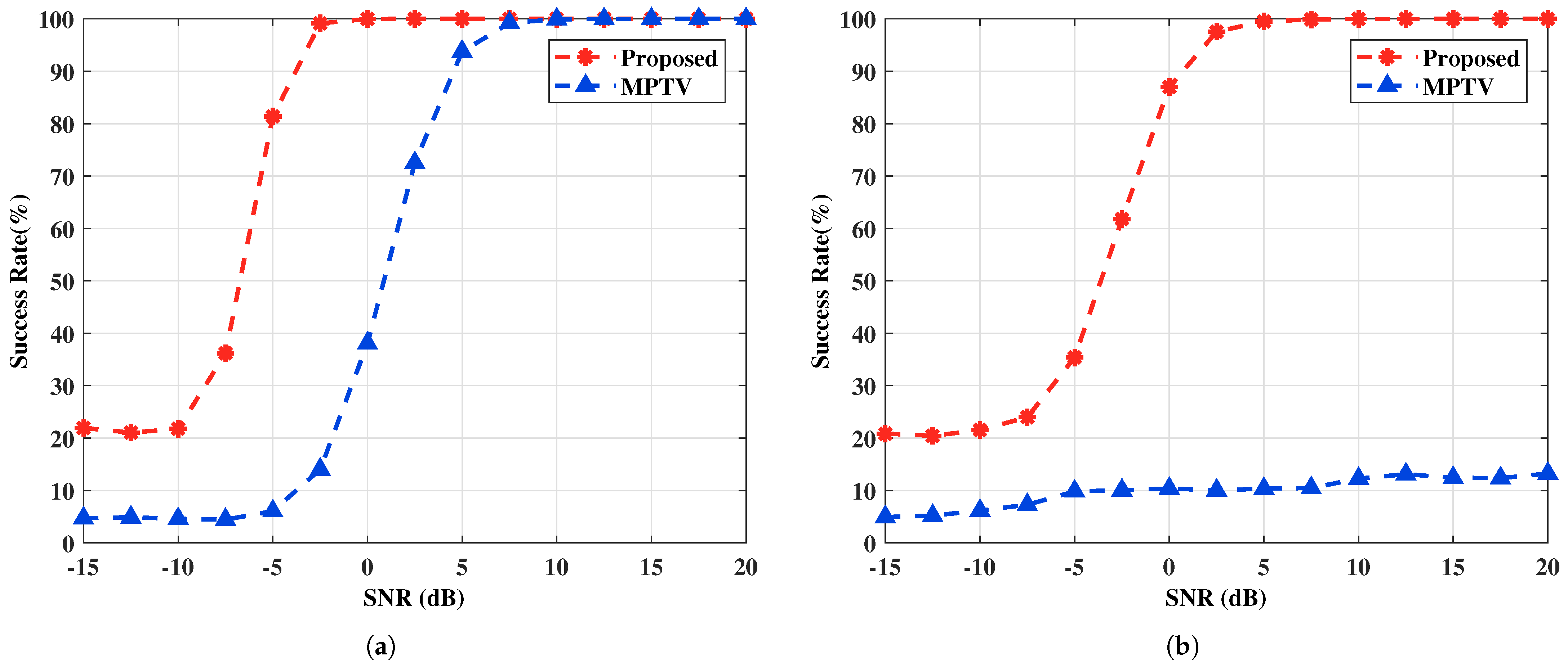
4.2.1. Performance vs. SNR: Example 1

In this example, the efficacy of the proposed method is evaluated in comparison to MPTV, with SNR values ranging from −15 to 20 dB in 2.5 dB increments. The number of subarray elements and the number of snapshots is set to $N=8$ and $J=50$, respectively. Let the amplitude and phase variation factor be ${\varpi }_k=1$ for $k=1,2,\cdots ,K$. To obtain accurate statistical characteristics of the method, 1000 Monte Carlo experiments are conducted for each fixed SNR. The experiments are conducted using two sets of targets with small and large angular intervals. Figure 4 and Figure 5 show the RMSE of DOA estimation versus SNR and the multi-target pairing success rate versus SNR for the two spatial target configurations.

It can be seen obviously from Figure 4 that the accuracy of angle estimation improves with increasing SNR, which concurrently enhances the multi-target pairing success rate, evident in Figure 5. As indicated by Equations (52) and (58), the dimensions of the constructed selection matrices differ, leading to variations in angle estimation performance for the two subarray azimuth angles, $\theta$ and $\phi$, in the proposed method. Specifically, the $S_1$-subarray demonstrates superior angle estimation performance compared to the $S_2$-subarray under low SNR and small angular interval target conditions. However, if we construct ${\mathbf{R}}_{z,x}=E\left\{\mathbf{Z}\left(n\right){\mathbf{X}}^H\left(n\right)\right\}$, the angle estimation performance of the two subarrays will reverse. Hence, if higher angle estimation performance is required for a specific subarray, the cross-correlation matrix can be constructed accordingly. The MPTV method exhibits low angular resolution, causing multiple target spectral peaks to merge together and become indistinguishable in scenarios with small angular interval targets, which leads to significant angle estimation errors and a low multi-target pairing success rate. For the two sets of spatial angles, the proposed method achieves a multi-target pairing success rate greater than 90% at SNR values above −4 dB and 1 dB, respectively. Furthermore, under the experimental conditions, the proposed method surpasses the MPTV method over SNR in both angle estimation accuracy and multi-target pairing success rate.

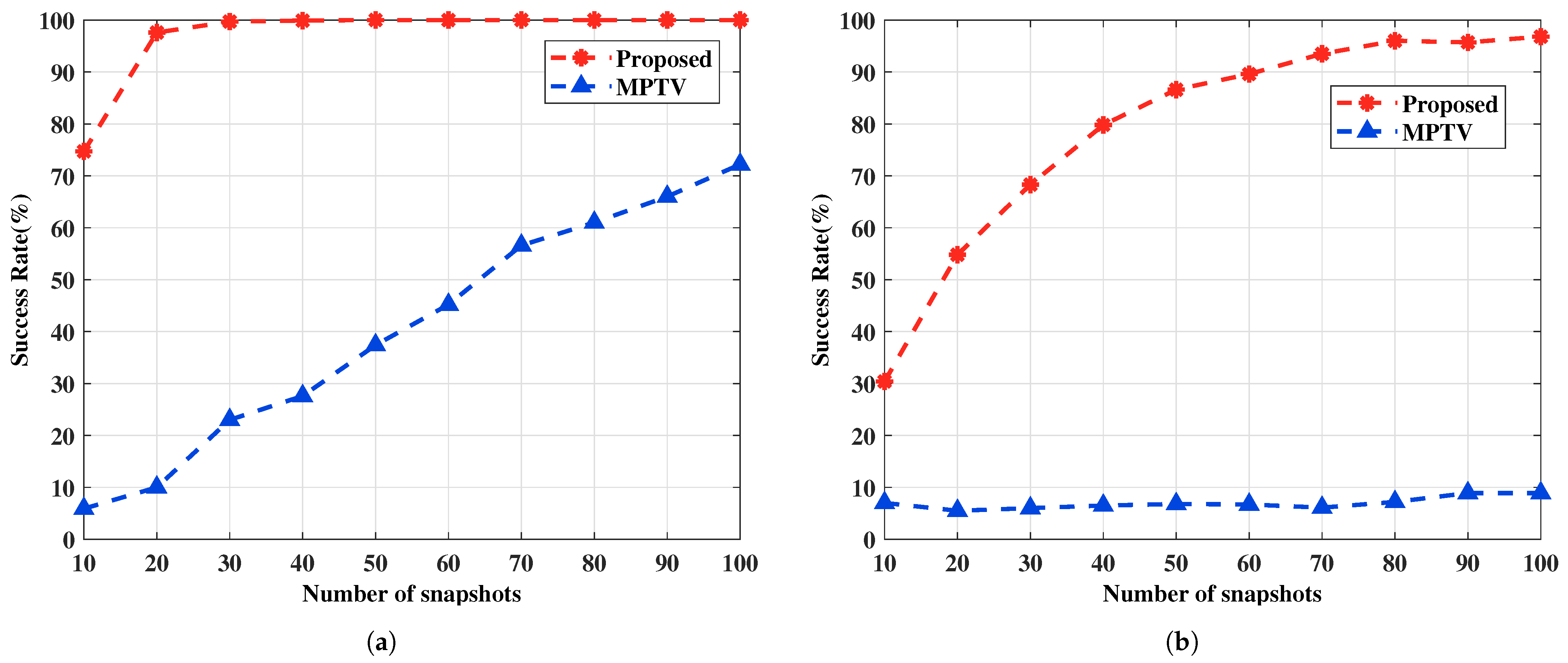
4.2.2. Performance vs. Number of Snapshots: Example 2

This example examines the impact of different numbers of snapshots on the performance of the proposed method and the comparative method MPTV. The SNR is fixed at SNR = 0 dB, and the number of snapshots J varies from 10 to 100 in intervals of 10. Other simulation conditions are the same as in Example 1. Every fixed J carries out 1000 Monte Carlo trials. Figure 6 and Figure 7 present the RMSE of DOA and the multi-target pairing success rate for the two sets of spatial angles, respectively.

As shown in Figure 6, it is evident that the angle estimation accuracy of the proposed method improves with an increasing number of snapshots. Additionally, irrespective of the target scenario involving large or small angular intervals, the RMSE curves of the proposed method remain consistently lower than those of the MPTV method. From Figure 7, it can be seen that a decrease in the number of snapshots increases the angle estimation error, thereby reducing the multi-target pairing success rate. Under the simulation conditions, the success rate of multi-target pairing surpasses 90% when the number of snapshots exceeds 15 and 60, respectively. In both sets of spatial target simulations, the proposed method exhibits better multi-target pairing performance compared to the MPTV method against the number of snapshots.

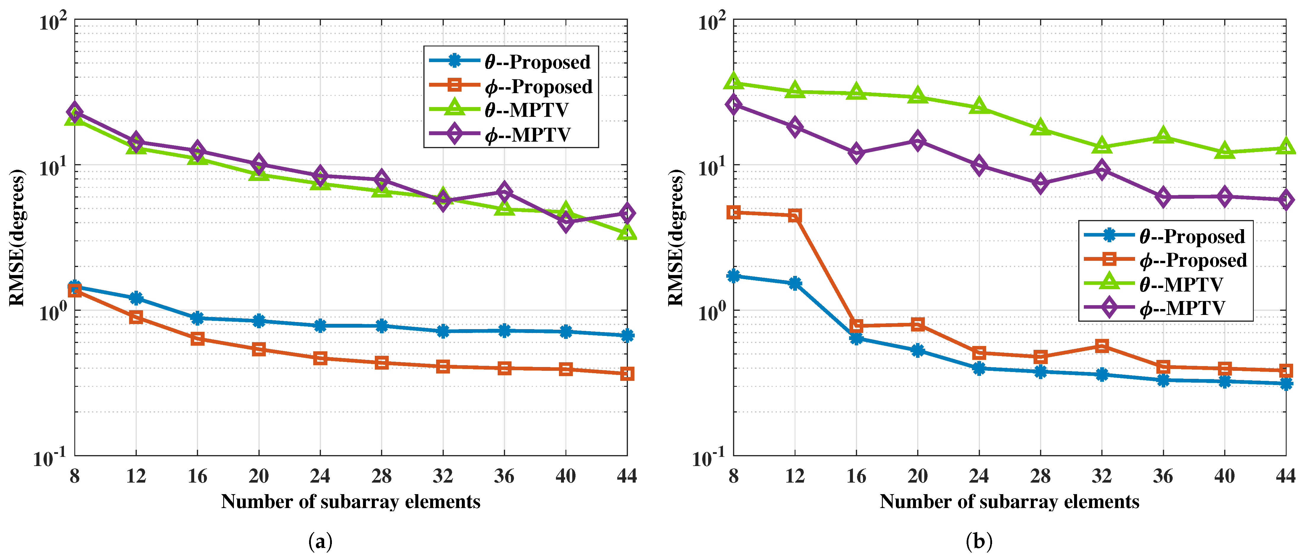
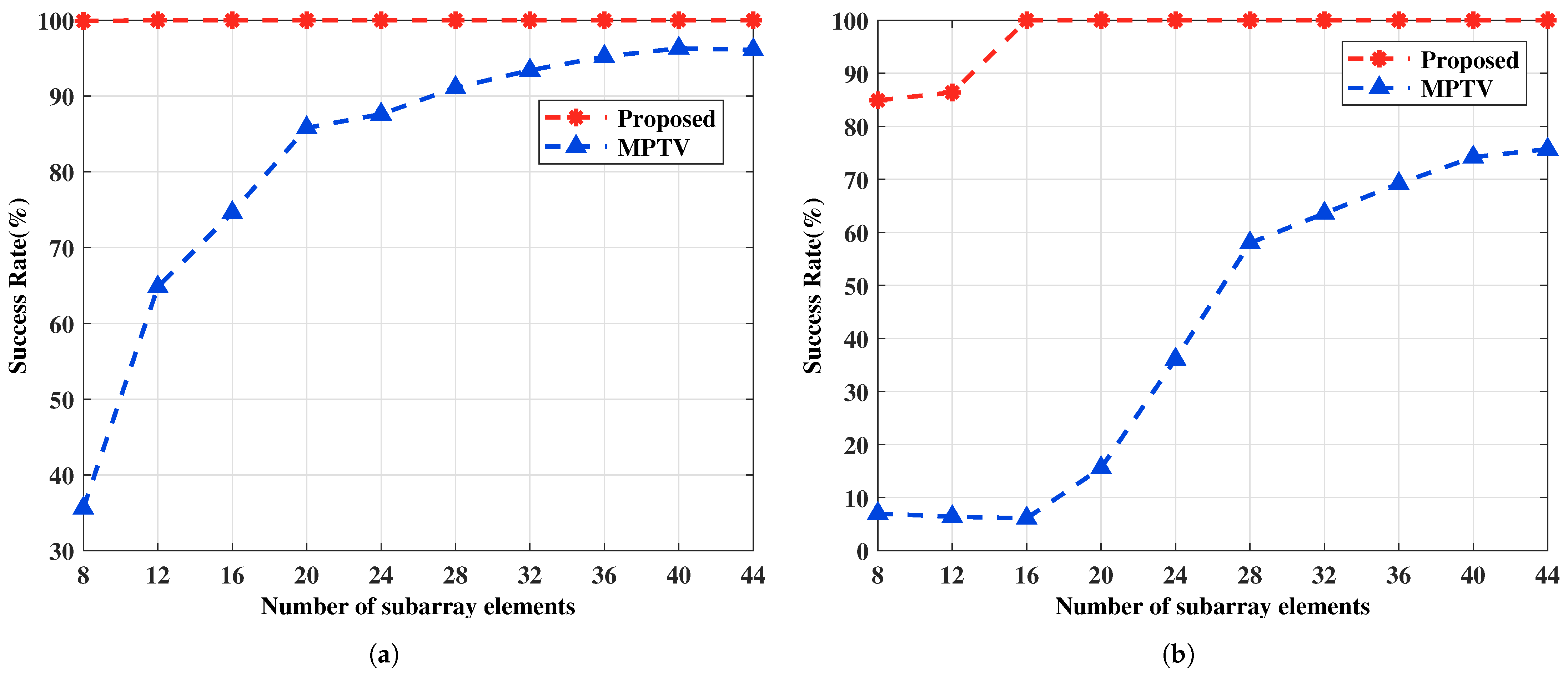
4.2.3. Performance vs. Number of Subarray Elements: Example 3

This example examines the impact of different numbers of snapshots on the performance of the proposed method and the comparative method MPTV. The SNR is fixed at SNR = 0 dB, and the number of snapshots J varies from 10 to 100 in intervals of 10. Other simulation conditions are the same as in Example 1. Every fixed J carries out 1000 Monte Carlo trials. The relationship between the RMSE of DOA estimation and the number of snapshots is shown in Figure 8, and the relationship between the multi-target pairing success rate and the number of snapshots is illustrated in Figure 9.

From Figure 8, it can be concluded that increasing the number of subarray elements results in a larger array aperture, which improves angle resolution and ultimately enhances the multi-target pairing success rate, as illustrated in Figure 9. The proposed method maintains a low angle estimation error and demonstrates superior multi-target pairing performance even with a limited number of subarray elements due to the utilization of generalized virtual array aperture extension technique. For both sets of spatial targets, the proposed method surpasses the MPTV method in terms of angle estimation accuracy and multi-target pairing performance with an identical quantity of subarray elements.

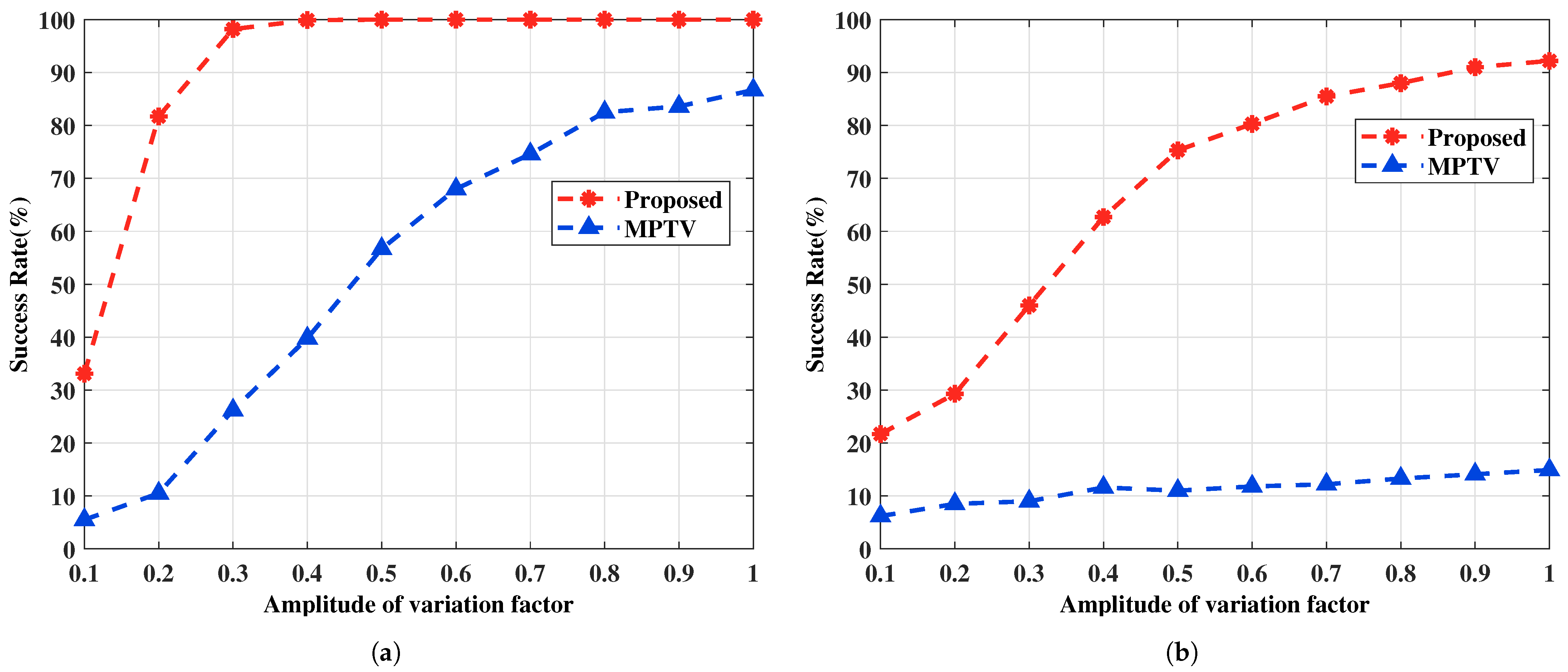
4.2.4. Performance vs. Amplitude and Phase Variation Factor: Example 4

In this example, we investigate the impact of the amplitude and phase variation factor ${\varpi }_k$ on the performance of the two methods. When the amplitude of the variation factor $\left|{\varpi }_k\right|$ is greater than 1, it is equivalent to swapping the positions of the two subarray data during signal processing compared to when $\left|{\varpi }_k\right|$ is less than 1. Therefore, simulations are conducted only for the case where $\left|{\varpi }_k\right|$ is less than 1. To facilitate the simulations and the presentation of results, the amplitude of the variation factors for all target signals is set to be identical, i.e., $\left|{\varpi }_1\right|=\left|{\varpi }_2\right|=\dots =\left|{\varpi }_K\right|$, with the amplitude increasing from 0.1 to 1 in increments of 0.1, and the phase of ${\varpi }_k$ uniformly distributed between 0 and $2\pi$. It is worth noting that the proposed method remains effective even when the amplitudes of the variation factors differ across targets. The SNR is set to 5 dB, and all other simulation conditions are consistent with those in Example 1. For each $\left|{\varpi }_k\right|$, 1000 Monte Carlo simulations are performed. Figure 10 and Figure 11 show the RMSE of DOA estimation and the pairing success rate under two sets of spatial targets.

Figure 10 and Figure 11 show that changes in the amplitude of the variation factor affect the accuracy of DOA estimation, which in turn impacts the success rate of multi-target pairing. As the amplitude of the variation decreases, the signal energy incident on the $S_2$-subarray after target reflection diminishes, resulting in greater angle estimation errors. It is also confirmed that the proposed method remains effective even when the target-reflected signals undergo amplitude and phase variations within a certain range at different angles, and it outperforms the MPTV method in both angle estimation and pairing performance.

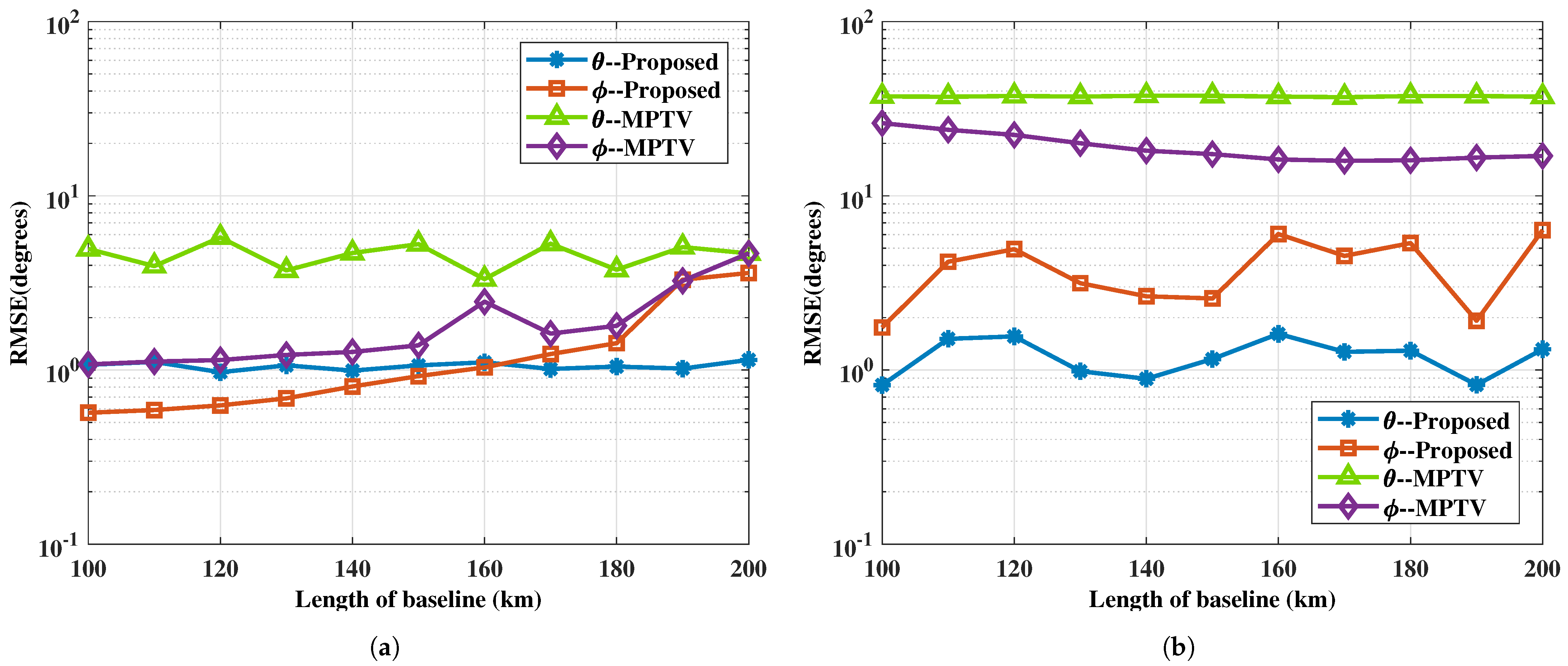
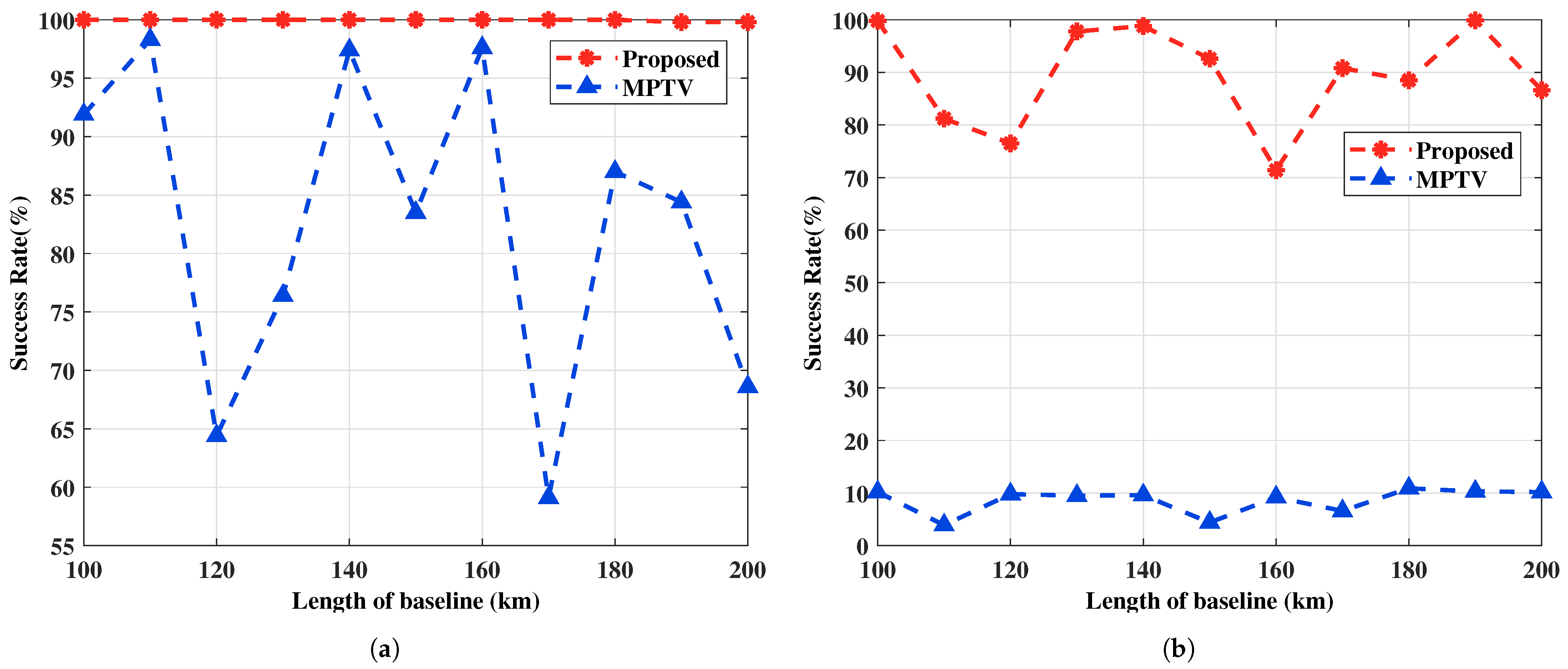
4.2.5. Performance vs. Length of Baseline: Example 5

In this example, we verify the performance of the proposed method compared to the MPTV method with respect to the length of the baseline. Fix SNR to 5 dB. Set the number of snapshots to $J=50$, configure the subarray elements to $N=8$, and let the amplitude and phase variation factor be ${\varpi }_k=1$ for $k=1,2,\dots ,K$. The coordinates of the $S_1$-subarray are $S_1\left(0,0\right)$ km, and the coordinates of the $S_2$-subarray vary from $\left(0,100\right)$ km to $\left(0,200\right)$ km in intervals of 10 km, with the length of baseline L correspondingly varying from 100 km to 200 km in increments of 10 km. A total of 1000 Monte Carlo experiments are carried out for each fixed L. Figure 12 depicts the RMSE of DOA estimation versus the length of baseline, and Figure 13 illustrates the multi-target pairing success rate versus the length of baseline, both for the two sets of target positions.

Figure 12 indicates that the length of the baseline impacts the accuracy of angle estimation, thereby affecting the multi-target pairing success rate, as shown in Figure 13. Specifically, changes in baseline length lead to variations in the amplitude and phase differences of the target signals incident on the two subarrays, indirectly modifying their power. Additionally, the azimuth angles of the S2-subarray also vary with the length of the baseline. The proposed method maintains a high pairing success rate for targets with large angular intervals under varying baseline lengths, whereas the MPTV method is more significantly affected. For targets with small angular intervals, the MPTV method fails to achieve effective multi-target pairing, while the proposed method maintains a pairing success rate of over 70%, despite fluctuations with changes in baseline length.

The preceding examples clearly demonstrate that the proposed method surpasses the MPTV method. This superiority is consistently demonstrated across simulations for both sets of spatial targets. In particular, the proposed method exhibits exceptional performance for small angular intervals and low SNR, owing to its utilization of rotational invariance and generalized aperture extension techniques.

5. Conclusions

In this paper, a computationally efficient multi-target pairing method is proposed to achieve multi-target pairing for further multi-target localization in T/R-R synergetic HFSWR. We calculate the amplitude and phase differences of the target signals impinging on the two subarrays for establishing and simplifying the cross-correlation matrix. In order to extract the rotation factor matrices containing multi-target pairing information and enhance performance, we develop a generalized array aperture extension technique. Ultimately, by combining the PM method and the ESPRIT algorithm, multi-target pairing is achieved using only angle information, with smaller RMSE of DOA estimation leading to higher multi-target pairing success rate. The proposed method overcomes the issues of grating lobes and angle ambiguity resulting from the long baseline. Unlike information-level fusion methods, it can be regarded as a DOA estimation method, falling under signal-level fusion techniques, which avoids multiframe association operations. Moreover, the proposed method does not involve spectral peak searching or iterations. Compared to existing similar methods, it has lower computational complexity while achieving better angle estimation and multi-target pairing performance, regardless of whether the spatial angle separation is large or small. Simulation results validate the method effectiveness and superior performance.

References

1. Li, J.; Yang, Q.; Zhang, X.; Ji, X.; Xiao, D. Space-Time Adaptive Processing Clutter-Suppression Algorithm Based on Beam Reshaping for High-Frequency Surface Wave Radar. Remote Sens. 2022, 14, 2935. [Google Scholar] [CrossRef]
2. Ji, Y.; Cheng, X.; Wang, Y.; Sun, W.; Zhang, X.; Jiang, M.; Ren, J.; Li, F. Motion compensation method using direct wave signal for CTSR bistatic HFSWR. IEEE Geosci. Remote Sens. Lett. 2023, 20, 1–5. [Google Scholar] [CrossRef]
3. Li, Y.; Wang, Z.; Zhang, W.; Lu, Z.; Xu, L.; Wang, Z. Joint correction method for ionospheric phase pollution of high-frequency sky-surface wave radar based on adaptive optimal path. IET Radar Sonar Navig. 2023, 17, 701–718. [Google Scholar] [CrossRef]
4. Yang, Z.; Lai, Y.; Zhou, H.; Tian, Y.; Qin, Y.; Lv, Z. Improving Ship Detection Based on Decision Tree Classification for High Frequency Surface Wave Radar. J. Mar. Sci. Eng. 2023, 11, 493. [Google Scholar] [CrossRef]
5. Sun, H. Conceptual study on bistatic shipborne high frequency surface wave radar. IEEE Aerosp. Electron. Syst. Mag. 2018, 33, 4–13. [Google Scholar] [CrossRef]
6. Wyatt, L.R.; Green, J.J.; Middleditch, A.; Moorhead, M.D.; Howarth, J.; Holt, M.; Keogh, S. Operational wave, current, and wind measurements with the Pisces HF radar. IEEE J. Ocean. Eng. 2006, 31, 819–834. [Google Scholar] [CrossRef]
7. Moo, P.; Ponsford, T.; DiFilippo, D.; McKerracher, R.; Kashyap, N.; Allard, Y. Canada’s Third Generation High Frequency Surface Wave Radar System. J. Ocean Technol. 2015, 10, 21. [Google Scholar]
8. Helzel, T.; Hansen, B.; Kniephoff, M.; Petersen, L.; Valentin, M. Introduction of the compact HF radar WERA-S. In Proceedings of the 2012 IEEE/OES Baltic International Symposium (BALTIC), Klaipeda, Lithuania, 8–10 May 2012; pp. 1–3. [Google Scholar]
9. Chuang, L.Z.; Chung, Y.J.; Tang, S. A simple ship echo identification procedure with SeaSonde HF radar. IEEE Geosci. Remote Sens. Lett. 2015, 12, 2491–2495. [Google Scholar] [CrossRef]
10. Sun, W.; Pang, Z.; Huang, W.; Ma, P.; Ji, Y.; Dai, Y.; Li, X. A multi-stage vessel tracklet association method for compact high-frequency surface wave radar. Remote Sens. 2022, 14, 1601. [Google Scholar] [CrossRef]
11. di Bisceglie, M.; Galdi, C. Ocean Remote Sensing Technologies: High frequency, marine and GNSS-based radar. In Ocean Remote Sensing Technologies: High Frequency, Marine and GNSS-Based Radar; IET The Institution of Engineering and Technology: Cambridge, UK, 2021. [Google Scholar]
12. Huang, W.; Gill, E.; Wu, X.; Li, L. Measurement of sea surface wind direction using bistatic high-frequency radar. IEEE Trans. Geosci. Remote Sens. 2012, 50, 4117–4122. [Google Scholar] [CrossRef]
13. Ji, Y.; Zhang, J.; Wang, Y.; Yue, C.; Gong, W.; Liu, J.; Sun, H.; Yu, C.; Li, M. Coast–ship bistatic HF surface wave radar: Simulation analysis and experimental verification. Remote Sens. 2020, 12, 470. [Google Scholar] [CrossRef]
14. Ji, Y.; Zhang, J.; Wang, Y.; Meng, J.; Yu, C.; Li, M.; Sun, W. Vessel target monitoring with bistatic compact HF surface wave radar. In Proceedings of the IGARSS 2020–2020 IEEE International Geoscience and Remote Sensing Symposium, Waikoloa, HI, USA, 17 February 2021; pp. 296–299. [Google Scholar]
15. Adve, R.S.; Applebaum, L.; Wicks, M.C.; Schneible, R.A. Space-time-waveform adaptive processing for frequency diverse distributed radar apertures. In Proceedings of the 2006 40th Annual Conference on Information Sciences and Systems, Princeton, NJ, USA, 22–24 March 2006; pp. 1413–1417. [Google Scholar]
16. Park, S.; Cho, C.J.; Lee, Y.; Da Costa, A.; Lee, S.; Ko, H. Coastal ship monitoring based on multiple compact high frequency surface wave radars. In Proceedings of the 2017 IEEE International Conference on Multisensor Fusion and Integration for Intelligent Systems (MFI), Daegu, Republic of Korea, 16–18 November 2017; pp. 565–569. [Google Scholar]
17. Lee, E.H.; Song, T.L. Multi-sensor track-to-track fusion with target existence in cluttered environments. IET Radar Sonar Navig. 2017, 11, 1108–1115. [Google Scholar] [CrossRef]
18. Zhao, K.; Yu, C.; Zhou, G.; Quan, T. Simultaneous Target Flying Mode Identification and Altitude Estimation in Bistatic T/R-R HFSWR. Asian J. Control 2016, 18, 1062–1074. [Google Scholar] [CrossRef]
19. Silva, M.T.; Shahidi, R.; Gill, E.W.; Huang, W. Nonlinear extraction of directional ocean wave spectrum from synthetic bistatic high-frequency surface wave radar data. IEEE J. Ocean. Eng. 2019, 45, 1004–1021. [Google Scholar] [CrossRef]
20. Ai, X.; Huang, Y.; Zhao, F.; Yang, J.; Li, Y.; Xiao, S. Imaging of spinning targets via narrow-band T/RR bistatic radars. IEEE Geosci. Remote Sens. Lett. 2012, 10, 362–366. [Google Scholar]
21. Sun, W.; Ji, M.; Huang, W.; Ji, Y.; Dai, Y. Vessel tracking using bistatic compact HFSWR. Remote Sens. 2020, 12, 1266. [Google Scholar] [CrossRef]
22. Sun, W.; Pang, Z.; Huang, W.; Ji, Y.; Dai, Y. Vessel velocity estimation and tracking from Doppler echoes of T/RR composite compact HFSWR. IEEE J. Sel. Top. Appl. Earth Obs. Remote Sens. 2021, 14, 4427–4440. [Google Scholar] [CrossRef]
23. Xu, B.; Zhao, Y. Transmit beamspace-based DOD and DOA estimation method for bistatic MIMO radar. Signal Process. 2019, 157, 88–96. [Google Scholar] [CrossRef]
24. Xu, B.; Zhao, Y. Joint transmit-receive B-PARAFAC method for angle estimation in bistatic MIMO radar. Digit. Signal Process. 2019, 92, 54–61. [Google Scholar] [CrossRef]
25. Dang, X.; Chen, B.; Yang, M.; Zheng, G. Beamspace unitary ESPRIT algorithm for angle estimation in bistatic MIMO radar. Int. J. Antennas Propag. 2015, 2015, 621358. [Google Scholar]
26. Hoffmann, R.; Neuberger, N.; Vehmas, R. Rx beamforming for long baseline multistatic radar networks. In Proceedings of the 2021 IEEE Radar Conference (RadarConf21), Atlanta, GA, USA, 7–14 May 2021; pp. 1–6. [Google Scholar]
27. Zhou, E.; Jiang, H.; Qi, H. 4-D parameter estimation in bistatic MIMO radar for near-field target localization. In Proceedings of the 2015 IEEE International Wireless Symposium (IWS 2015), Shenzhen, China, 30 March–1 April 2015; pp. 1–4. [Google Scholar]
28. Wang, S.; Feng, J.; Wang, F.; Zhang, J.; Liang, X. Research on location accuracy in bistatic radar network. In Proceedings of the 2011 IEEE 2nd International Conference on Computing, Control and Industrial Engineering, Wuhan, China, 20–21 August 2011; Volume 1, pp. 98–101. [Google Scholar]
29. Sun, W.; Li, X.; Pang, Z.; Ji, Y.; Dai, Y.; Huang, W. Track-to-Track association based on maximum likelihood estimation for T/RR composite compact HFSWR. IEEE Trans. Geosci. Remote Sens. 2023, 61, 1–12. [Google Scholar]
30. Xu, Z.; Fang, L. An improved track association algorithm based on AdaBoost and decision tree. In Proceedings of the 2021 4th International Conference on Advanced Electronic Materials, Computers and Software Engineering (AEMCSE), Changsha, China, 26–28 March 2021; pp. 794–800. [Google Scholar]
31. Chen, T.; Yang, P.; Peng, H.; Qian, Z. Multi-target tracking algorithm based on PHD filter against multi-range-false-target jamming. J. Syst. Eng. Electron. 2020, 31, 859–870. [Google Scholar] [CrossRef]
32. Tang, H.; Zhao, Y.; Wang, Y. The multi-target association algorithm based on multi-feature. In Proceedings of the 2018 IEEE International Conference on Computational Electromagnetics (ICCEM), Chengdu, China, 26–28 March 2018; pp. 1–3. [Google Scholar]
33. Hao, L. A possibilistic data association based algorithm for multi-target tracking. In Proceedings of the 2013 Third International Conference on Intelligent System Design and Engineering Applications, Hong Kong, China, 16–18 January 2013; pp. 158–162. [Google Scholar]
34. Bai, Y.; Wu, X.; Deng, W.; Zhang, X. Multi-target pair-matching method based on angle information in transmit/receive-receive synergetic High Frequency Surface Wave Radar. IET Radar Sonar Navig. 2022, 16, 1188–1197. [Google Scholar] [CrossRef]
35. Wu, R.; Zhang, Z. Convex optimization-based 2-D DOA estimation with enhanced virtual aperture and virtual snapshots extension for l-shaped array. IEEE Trans. Veh. Technol. 2020, 69, 6473–6484. [Google Scholar] [CrossRef]
36. Dong, Y.Y.; Dong, C.x.; Xu, J.; Zhao, G.q. Computationally efficient 2-D DOA estimation for L-shaped array with automatic pairing. IEEE Antennas Wirel. Propag. Lett. 2016, 15, 1669–1672. [Google Scholar] [CrossRef]
37. Nie, X.; Li, L. A computationally efficient subspace algorithm for 2-D DOA estimation with L-shaped array. IEEE Signal Process. Lett. 2014, 21, 971–974. [Google Scholar]
38. Wang, G.; Xin, J.; Wang, J.; Zheng, N.; Sano, A. Subspace-based two-dimensional direction estimation and tracking of multiple targets. IEEE Trans. Aerosp. Electron. Syst. 2015, 51, 1386–1402. [Google Scholar] [CrossRef]
39. Cui, M.; Dai, L. Channel estimation for extremely large-scale MIMO: Far-field or near-field? IEEE Trans. Commun. 2022, 70, 2663–2677. [Google Scholar] [CrossRef]
40. Mailloux, R.J. Phased Array Antenna Handbook; Artech House: Norwood, MA, USA, 2017. [Google Scholar]
41. Ryan, J.G.; Goubran, R.A. Array optimization applied in the near field of a microphone array. IEEE Trans. Speech Audio Process. 2000, 8, 173–176. [Google Scholar] [CrossRef]
Figure 1. (a) System configuration of traditional HFSWR. (b) System configuration of T/R-R synergetic HFSWR.
Remotesensing 16 03128 g001
Figure 2. Dual receiving arrays model.
Remotesensing 16 03128 g002
Figure 3. Distinction between the far-field and the near-field regions.
Remotesensing 16 03128 g003
Figure 4. The RMSE of DOA estimation versus SNR. (a) K = 3 with large angular intervals ( 80.53 , 116.56 ) , ( 45.00 , 135.00 ) , ( 63.43 , 99.46 ) , N = 8 , J = 50 . (b) K = 3 with small angular intervals ( 77.79 , 93.09 ) , ( 81.86 , 102.09 ) , ( 86.18 , 124.15 ) , N = 8 and J = 50 .
Remotesensing 16 03128 g004
Figure 5. The multi-target pairing success rate versus SNR. (a) K = 3 with large angular intervals ( 80.53 , 116.56 ) , ( 45.00 , 135.00 ) , ( 63.43 , 99.46 ) , N = 8 , J = 50 . (b) K = 3 with small angular intervals ( 77.79 , 93.09 ) , ( 81.86 , 102.09 ) , ( 86.18 , 124.15 ) , N = 8 and J = 50 .
Remotesensing 16 03128 g005
Figure 6. The RMSE of DOA estimation versus the number of snapshots. (a) K = 3 with large angular intervals ( 80.53 , 116.56 ) , ( 45.00 , 135.00 ) , ( 63.43 , 99.46 ) , N = 8 , SNR = 0 dB. (b) K = 3 with small angular intervals ( 77.79 , 93.09 ) , ( 81.86 , 102.09 ) , ( 86.18 , 124.15 ) , N = 8 and SNR = 0 dB.
Remotesensing 16 03128 g006
Figure 7. The multi-target pairing success rate versus the number of snapshots. (a) K = 3 with large angular intervals ( 80.53 , 116.56 ) , ( 45.00 , 135.00 ) , ( 63.43 , 99.46 ) , N = 8 , SNR = 0 dB. (b) K = 3 with small angular intervals ( 77.79 , 93.09 ) , ( 81.86 , 102.09 ) , ( 86.18 , 124.15 ) , N = 8 , SNR = 0 dB.
Remotesensing 16 03128 g007
Figure 8. The RMSE of DOA estimation versus the number of subarray elements. (a) K = 3 with large angular intervals ( 80.53 , 116.56 ) , ( 45.00 , 135.00 ) , ( 63.43 , 99.46 ) , J = 50 , SNR = 0 dB. (b) K = 3 with small angular intervals ( 77.79 , 93.09 ) , ( 81.86 , 102.09 ) , ( 86.18 , 124.15 ) , J = 50 , SNR = 0 dB.
Remotesensing 16 03128 g008
Figure 9. The multi-target pairing success rate versus the number of subarray elements. (a) K = 3 with large angular intervals ( 80.53 , 116.56 ) , ( 45.00 , 135.00 ) , ( 63.43 , 99.46 ) , J = 50 , SNR = 0 dB. (b) K = 3 with small angular intervals ( 77.79 , 93.09 ) , ( 81.86 , 102.09 ) , ( 86.18 , 124.15 ) , J = 50 and SNR = 0 dB.
Remotesensing 16 03128 g009
Figure 10. The RMSE of DOA estimation versus the amplitude of variation factor. (a) K = 3 with large angular intervals ( 80.53 , 116.56 ) , ( 45.00 , 135.00 ) , ( 63.43 , 99.46 ) , N = 8 , J = 50 , SNR = 5 dB. (b) K = 3 with small angular intervals ( 77.79 , 93.09 ) , ( 81.86 , 102.09 ) , ( 86.18 , 124.15 ) , N = 8 , J = 50 , SNR = 5 dB.
Remotesensing 16 03128 g010
Figure 11. The multi-target pairing success rate versus the amplitude of variation factor. (a) K = 3 with large angular intervals ( 80.53 , 116.56 ) , ( 45.00 , 135.00 ) , ( 63.43 , 99.46 ) , N = 8 , J = 50 , SNR = 5 dB. (b) K = 3 with small angular intervals ( 77.79 , 93.09 ) , ( 81.86 , 102.09 ) , ( 86.18 , 124.15 ) , N = 8 , J = 50 , SNR = 5 dB.
Remotesensing 16 03128 g011
Figure 12. The RMSE of DOA estimation versus the length of baseline. (a) K = 3 with large angular intervals, N = 8 , J = 50 , SNR = 5 dB. (b) K = 3 with small angular intervals, N = 8 , J = 50 and SNR = 5 dB.
Remotesensing 16 03128 g012
Figure 13. The multi-target pairing success rate versus the length of baseline. (a) K = 3 with large angular intervals, N = 8 , J = 50 , SNR = 5 dB. (b) K = 3 with small angular intervals, N = 8 , J = 50 and SNR = 5 dB.
Remotesensing 16 03128 g013
Disclaimer/Publisher’s Note: The statements, opinions and data contained in all publications are solely those of the individual author(s) and contributor(s) and not of MDPI and/or the editor(s). MDPI and/or the editor(s) disclaim responsibility for any injury to people or property resulting from any ideas, methods, instructions or products referred to in the content.