
Modeling the Long-Term Variability in the Surfaces of Three Lakes in Morocco with Limited Remote Sensing Image Sources

 , , and
Abstract
:1. Introduction
2. Data
3. Interpolation Methodology
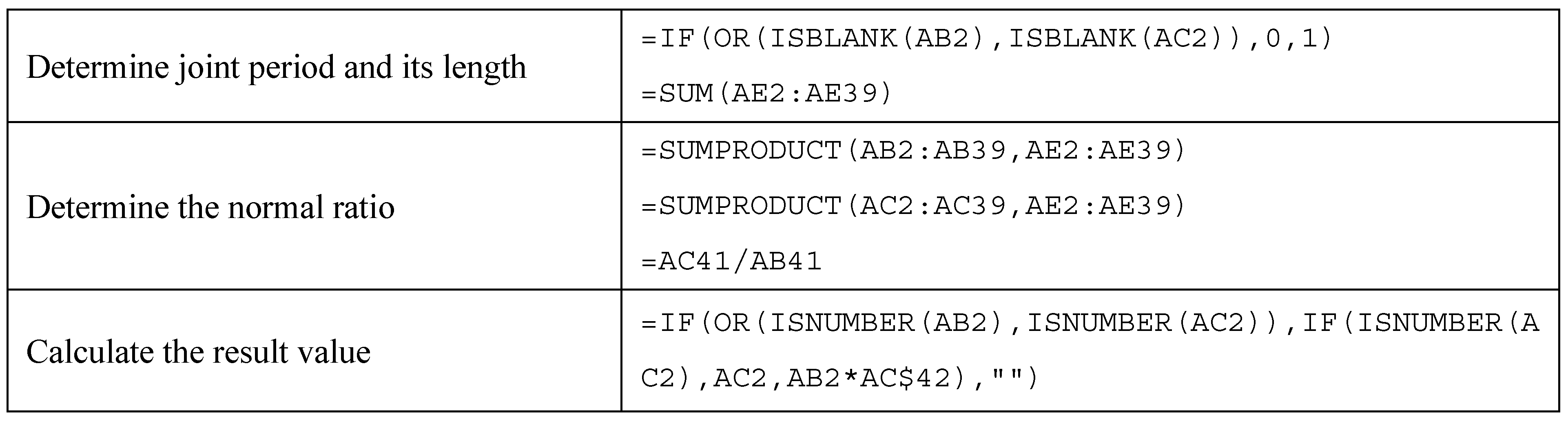
3.1. The Iterative Ratio Method
- N—joint period length;
- xi, yi—values at reference at missing location.
- NR—calculated normal ratio;
- yk—missing value;
- xk—existing value at a different location.
3.2. Kalman Filter
4. Results
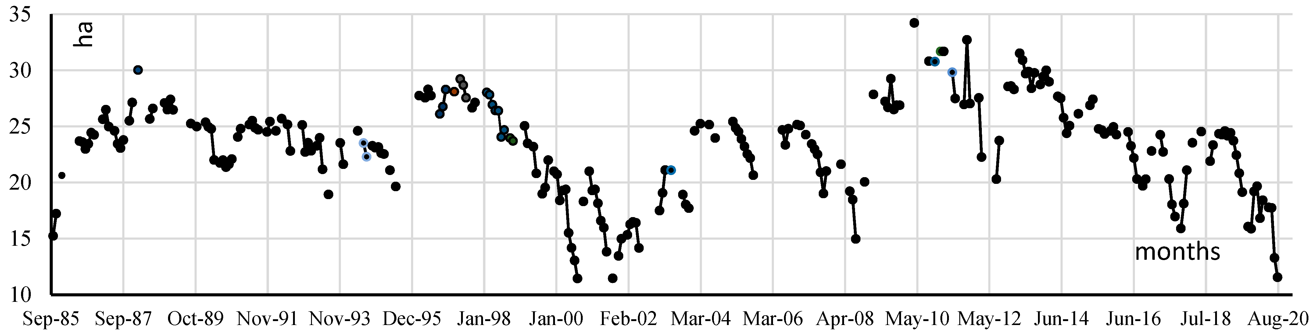
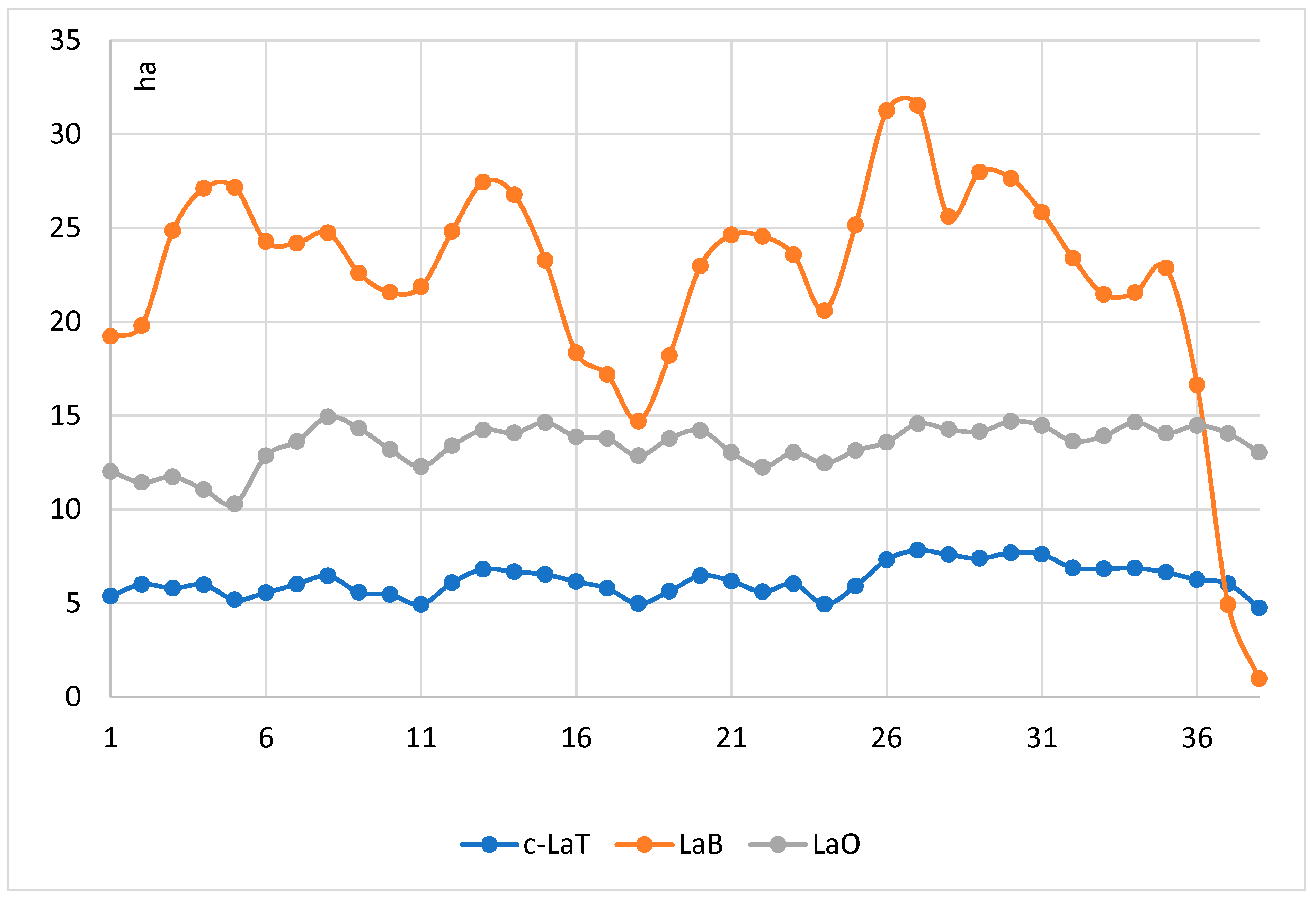
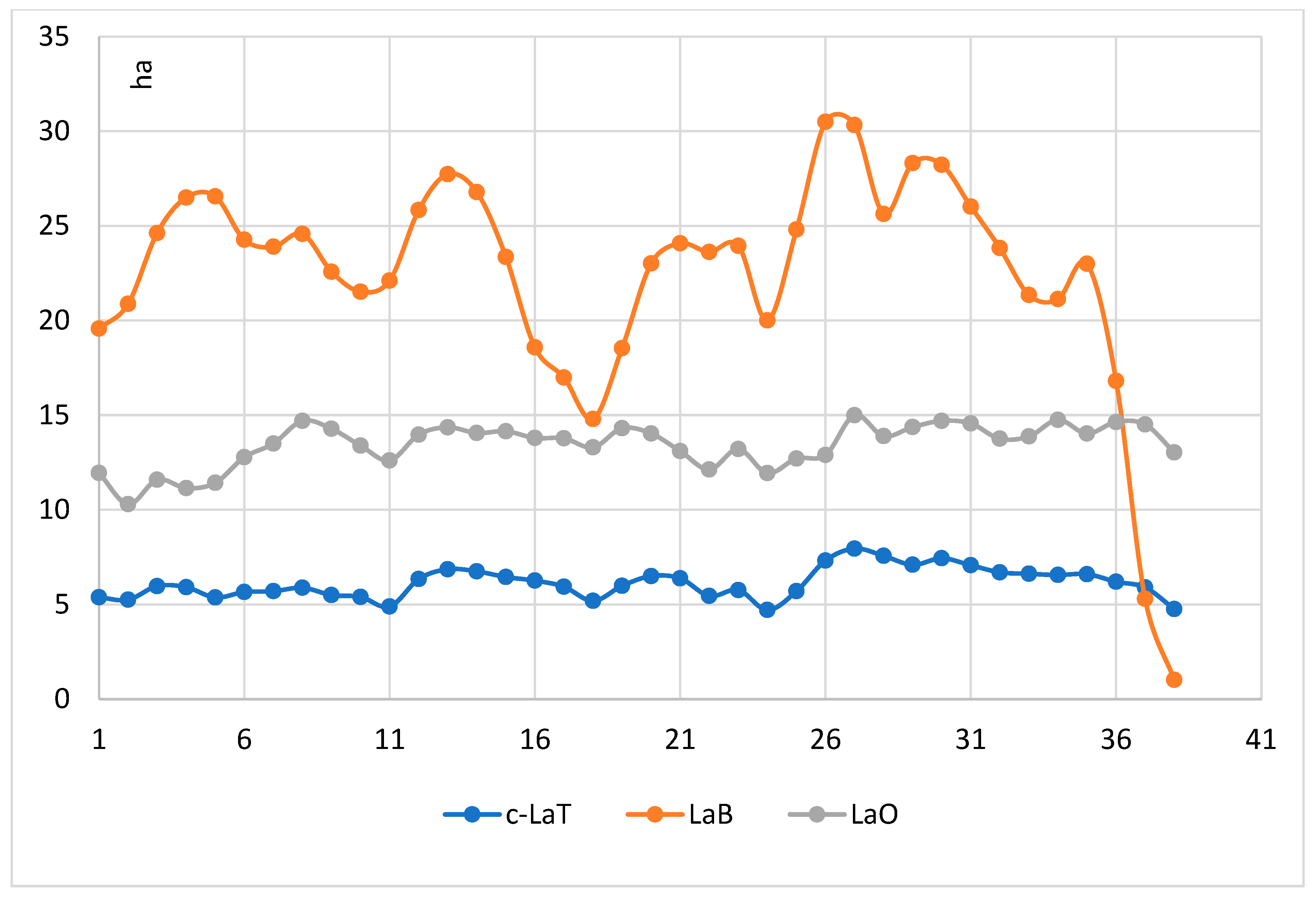
4.1. LaB Case
4.2. LaO Case
4.3. c-LaT Case
5. Discussion
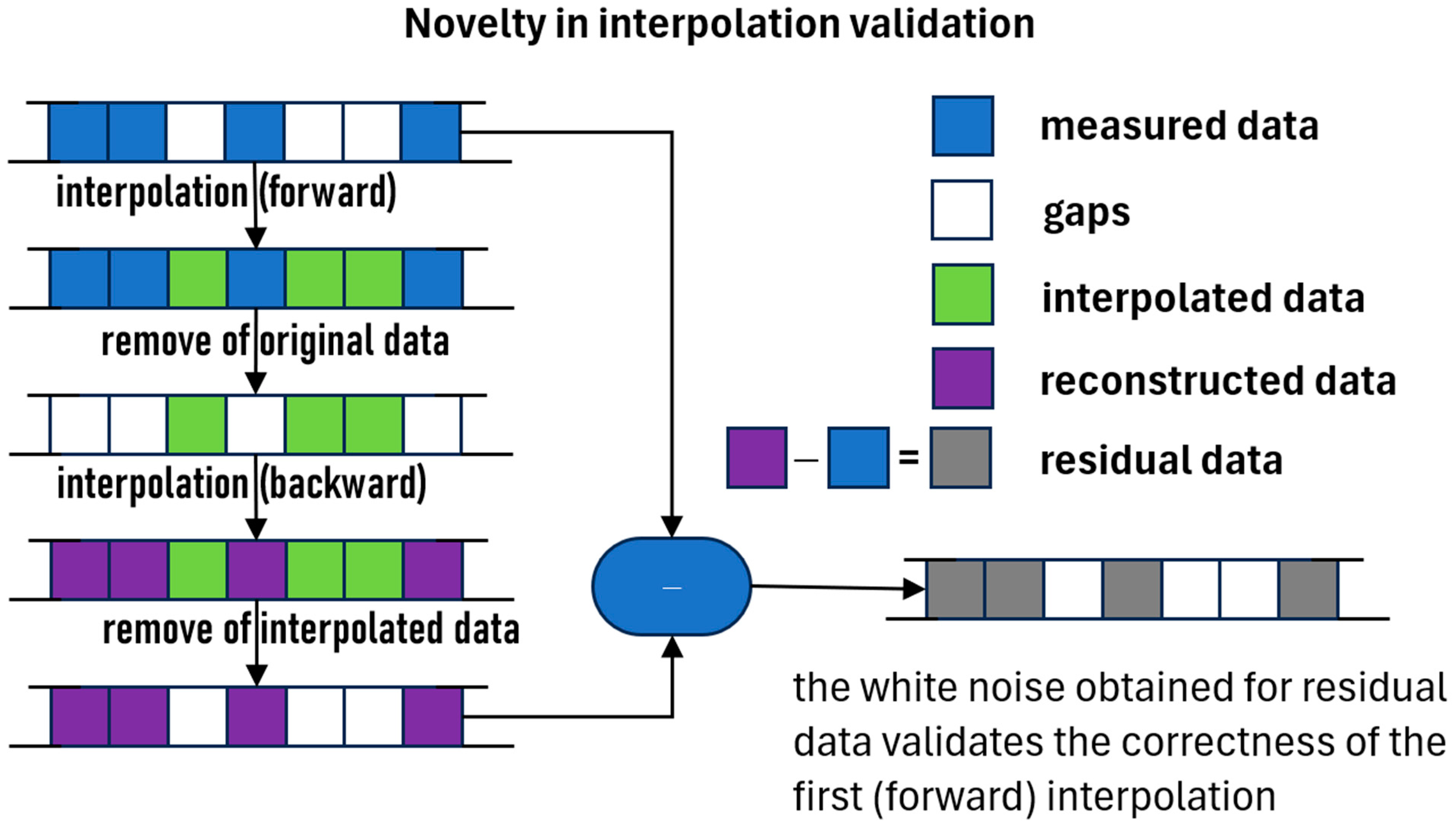
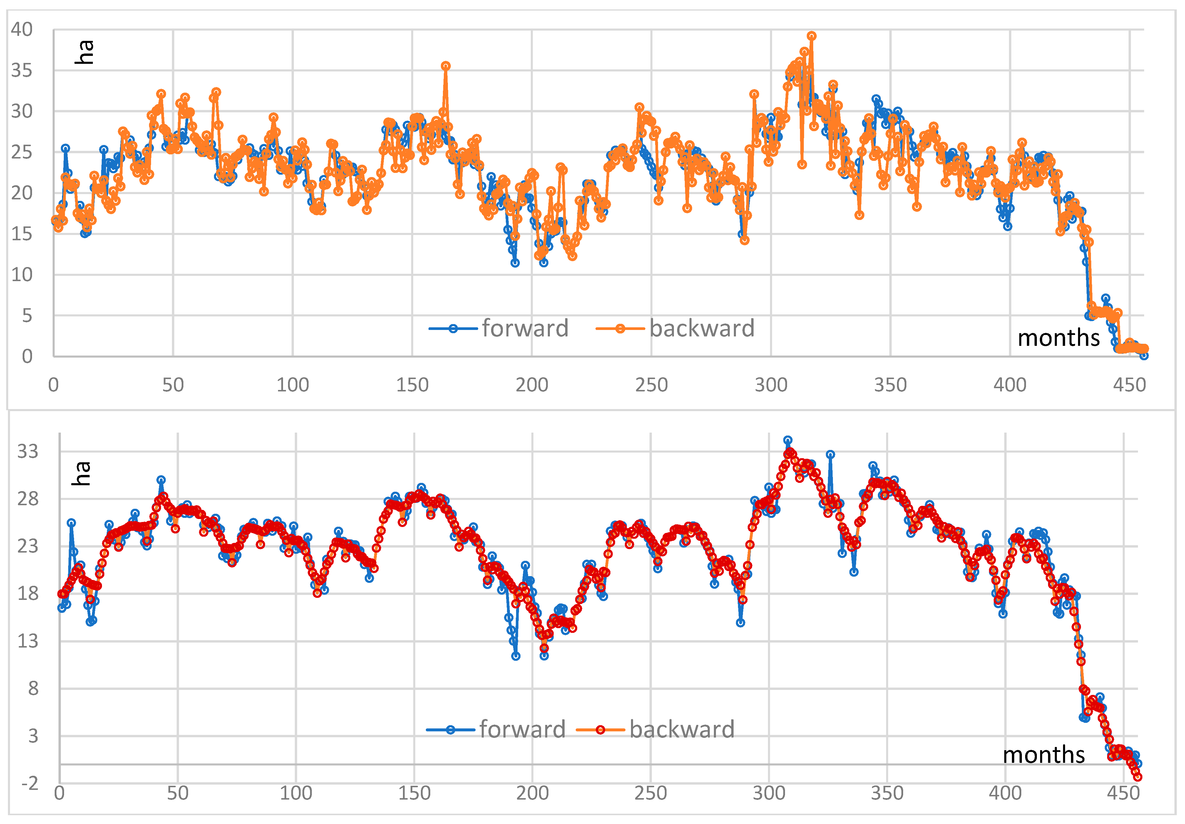
5.1. Discussion on the Interpolation Validation
5.2. Discussion on the Obtained Results
6. Conclusions
Author Contributions
Funding
Data Availability Statement
Acknowledgments
Conflicts of Interest
References
- Everhardt, B.A. Great Lakes Water Resources: Planning for the Nation’s Future. Toledo J. Gt. Lakes Law Sci. Policy 2001, 3, 90–111. [Google Scholar]
- Mleczko, M.; Mróz, M. Wetland Mapping Using SAR Data from the Sentinel-1A and TanDEM-X Missions: A Comparative Study in the Biebrza Floodplain (Poland). Remote Sens. 2018, 10, 78. [Google Scholar] [CrossRef]
- Mishra, A.K.; Singh, V.P. A Review of Drought Concepts. J. Hydrol. 2010, 391, 202–216. [Google Scholar] [CrossRef]
- El-Bouhali, A.; Amyay, M.; Ech-Chahdi, K.E.O. Changes in water surface area of the Middle Atlas-Morocco lakes: A response to climate and human effects. IJEG 2024, 9, 221–232. [Google Scholar] [CrossRef]
- Bai, M.; Mo, X.; Liu, S.; Hu, S. Detection and Attribution of Lake Water Loss in the Semi-Arid Mongolian Plateau-A Case Study in the Lake Dalinor. Ecohydrology 2021, 14, e2251. [Google Scholar] [CrossRef]
- Duan, Z.; Bastiaanssen, W.G.M. Estimating Water Volume Variations in Lakes and Reservoirs from Four Operational Satellite Altimetry Databases and Satellite Imagery Data. Remote Sens. Environ. 2013, 134, 403–416. [Google Scholar] [CrossRef]
- White, L.; Brisco, B.; Dabboor, M.; Schmitt, A.; Pratt, A. A Collection of SAR Methodologies for Monitoring Wetlands. Remote Sens. 2015, 7, 7615–7645. [Google Scholar] [CrossRef]
- Zhao, Z.; Liu, F.; Zhang, Y.; Liu, L.; Qi, W. The Dynamic Response of Lakes in the Tuohepingco Basin of the Tibetan Plateau to Climate Change. Environ. Earth Sci. 2017, 76, 137. [Google Scholar] [CrossRef]
- Yao, F.; Wang, J.; Wang, C.; Crétaux, J.-F. Constructing Long-Term High-Frequency Time Series of Global Lake and Reservoir Areas Using Landsat Imagery. Remote Sens. Environ. 2019, 232, 111210. [Google Scholar] [CrossRef]
- Liu, K.; Song, C.; Wang, J.; Ke, L.; Zhu, Y.; Zhu, J.; Ma, R.; Luo, Z. Remote Sensing-Based Modeling of the Bathymetry and Water Storage for Channel-Type Reservoirs Worldwide. Water Resour. Res. 2020, 56, e2020WR027147. [Google Scholar] [CrossRef]
- Chen, T.; Song, C.; Ke, L.; Wang, J.; Liu, K.; Wu, Q. Estimating Seasonal Water Budgets in Global Lakes by Using Multi-Source Remote Sensing Measurements. J. Hydrol. 2021, 593, 125781. [Google Scholar] [CrossRef]
- Ahmed, I.A.; Shahfahad, S.; Baig, M.R.I.; Talukdar, S.; Asgher, M.S.; Usmani, T.M.; Ahmed, S.; Rahman, A. Lake Water Volume Calculation Using Time Series LANDSAT Satellite Data: A Geospatial Analysis of Deepor Beel Lake, Guwahati. Front. Eng. Built Environ. 2021, 1, 107–130. [Google Scholar] [CrossRef]
- Pi, X.; Luo, Q.; Feng, L.; Xu, Y.; Tang, J.; Liang, X.; Ma, E.; Cheng, R.; Fensholt, R.; Brandt, M.; et al. Mapping Global Lake Dynamics Reveals the Emerging Roles of Small Lakes. Nat. Commun. 2022, 13, 5777. [Google Scholar] [CrossRef]
- Zhao, G.; Li, Y.; Zhou, L.; Gao, H. Evaporative Water Loss of 1.42 Million Global Lakes. Nat. Commun. 2022, 13, 3686. [Google Scholar] [CrossRef] [PubMed]
- Zhao, W.; Xiong, D.; Wen, F.; Wang, X. Lake Area Monitoring Based on Land Surface Temperature in the Tibetan Plateau from 2000 to 2018. Environ. Res. Lett. 2020, 15, 084033. [Google Scholar] [CrossRef]
- Gao, S.; He, D.; Zhang, Z.; Tang, X.; Zhao, Z. A novel dynamic interpolation method based on both temporal and spatial correlations. Appl Intell. 2023, 53, 5100–5125. [Google Scholar] [CrossRef]
- Lepot, M.; Aubin, J.B.; Clemens, F.H. Clemens, Interpolation in Time Series: An Introductive Overview of Existing Methods, Their Performance Criteria and Uncertainty Assessment. Water 2017, 9, 10. [Google Scholar] [CrossRef]
- Qin, R.; Chen, G.; Zhang, H.; Liu, L.; Long, S. A Kalman Filter-Based Method for Reconstructing GMS-5 Land Surface Temperature Time Series. Appl. Sci. 2022, 12, 15. [Google Scholar] [CrossRef]
- Shi, Q.; Dai, W.; Santerre, R.; Liu, N. A Modified Spatiotemporal Mixed-Effects Model for Interpolating Missing Values in Spatiotemporal Observation Data Series. Math. Probl. Eng. 2020, 2020, 1070831. [Google Scholar] [CrossRef]
- Arun, P.V. A comparative analysis of different DEM interpolation methods. Egypt J. Remote Sens. Space Sci. 2013, 16, 133–139. [Google Scholar] [CrossRef]
- Huber, F.; Schulz, S.; Steinhage, V. Deep Interpolation of Remote Sensing Land Surface Temperature Data with Partial Convolutions. Sensors 2024, 24, 5. [Google Scholar] [CrossRef] [PubMed]
- Martin, J.; Jover, H.; Le Coz, J.; Maurer, J.; Noin, D. Géographie du Maroc; Hatier: Paris, France, 1964. [Google Scholar]
- Baali, A. Genèse et Évolution Au Plio-Quaternaire de Deux Bassins Intram-Ontagneux en Domaine Carbonaté Méditerranéen. Les Bassins Versants Des Dayets (Lacs) Afourgagh et Agoulmam (Moyen Atlas, Maroc). Thesis, Université Sidi Mohamed Ben Abdellah, Fès, Morocco, 1998. [Google Scholar]
- Detriche, S. Evolution D’un Système Lacustre Karstique au Cours de la Période Historique D’après L’étude des Archives Sédimentaires: La Dayet Afourgagh (Moyen-Atlas, Maroc). Ph.D. Thesis, Université François Rabelais de Tours, Tours, France, 2007. [Google Scholar]
- Gouiss, A.; Taybi, Y.; Gharmane, Y.; M’Rabet, S. Contribution of Space Remote Sensing and New Gis Tools for Mapping Geological Structures in the Mekkam Region of Northeast Morocco. Geogr. Tech. 2023, 18, 149–157. [Google Scholar] [CrossRef]
- Chillasse, L.; Dakki, M.; Abbassi, M. Valeurs et fonctions écologiques des Zones humides du Moyen Atlas (Maroc). Humed. Mediterráneos 2001, 1, 139–146. [Google Scholar]
- ABHOER. Atlas des Sources et Lacs; Agence du Bassin Hydraulique de l’Oum Er Rbia: Beni Mellal, Morocco, 2019; p. 119. [Google Scholar]
- Chillasse, L.; Dakki, M. Potentialités et Statuts de Conservation Des Zones Humides Du Moyen-Atlas (Maroc), Avec Référence Aux Influences de La Sécheresse. Sci. Chang. Planétaires Sécher. 2004, 15, 337–345. [Google Scholar]
- Benkaddour, A. Changements Hydrologiques et Climatiques Dans Le Moyen-Atlas Marocain, Chronologie, Minéralogie, Géochimie Isotopique et Élémentaire Des Sédiments Lacustres de Tigalmamine. Ph.D. Thesis, Université Paris-Sud, Orsay, France, 1993. [Google Scholar]
- Bonnema, M.; Hossain, F. Inferring Reservoir Operating Patterns across the Mekong Basin Using Only Space Observations. WATER Resour. Res. 2017, 53, 3791–3810. [Google Scholar] [CrossRef]
- Xing, L.; Tang, X.; Wang, H.; Fan, W.; Gao, X. Mapping Wetlands of Dongting Lake in China Using Landsat and Sentinel-1 Time Series at 30 M. Int. Arch. Photogramm. Remote Sens. Spat. Inf. Sci. 2018, 42, 1971–1976. [Google Scholar] [CrossRef]
- Slagter, B.; Tsendbazar, N.-E.; Vollrath, A.; Reiche, J. Mapping Wetland Characteristics Using Temporally Dense Sentinel-1 and Sentinel-2 Data: A Case Study in the St. Lucia Wetlands, South Africa. Int. J. Appl. Earth Obs. Geoinf. 2020, 86, 102009. [Google Scholar] [CrossRef]
- Han, X.; Chen, X.; Feng, L. Four Decades of Winter Wetland Changes in Poyang Lake Based on Landsat Observations between 1973 and 2013. Remote Sens. Environ. 2015, 156, 426–437. [Google Scholar] [CrossRef]
- Song, C.; Huang, B.; Ke, L.; Richards, K.S. Remote Sensing of Alpine Lake Water Environment Changes on the Tibetan Plateau and Surroundings: A Review. ISPRS J. Photogramm. Remote Sens. 2014, 92, 26–37. [Google Scholar] [CrossRef]
- Dörnhöfer, K.; Oppelt, N. Remote Sensing for Lake Research and Monitoring—Recent Advances. Ecol. Indic. 2016, 64, 105–122. [Google Scholar] [CrossRef]
- Lin, Y.; Li, X.; Zhang, T.; Chao, N.; Yu, J.; Cai, J.; Sneeuw, N. Water Volume Variations Estimation and Analysis Using Multisource Satellite Data: A Case Study of Lake Victoria. Remote Sens. 2020, 12, 3052. [Google Scholar] [CrossRef]
- Kang, J.; Guan, H.; Peng, D.; Chen, Z. Multi-Scale Context Extractor Network for Water-Body Extraction from High-Resolution Optical Remotely Sensed Images. Int. J. Appl. Earth Obs. Geoinf. 2021, 103, 102499. [Google Scholar] [CrossRef]
- Xu, H. Modification of Normalised Difference Water Index (NDWI) to Enhance Open Water Features in Remotely Sensed Imagery. Int. J. Remote Sens. 2006, 27, 3025–3033. [Google Scholar] [CrossRef]
- Li, W.; Du, Z.; Ling, F.; Zhou, D.; Wang, H.; Gui, Y.; Sun, B.; Zhang, X. A Comparison of Land Surface Water Mapping Using the Normalized Difference Water Index from TM, ETM+ and ALI. Remote Sens. 2013, 5, 5530–5549. [Google Scholar] [CrossRef]
- Du, Z.; Li, W.; Zhou, D.; Tian, L.; Ling, F.; Wang, H.; Gul, Y.; Sun, B. Analysis of Landsat-8 OLI Imagery for Land Surface Water Mapping. Remote Sens. Lett. 2014, 5, 672–681. [Google Scholar] [CrossRef]
- Singh, K.V.; Setia, R.; Sahoo, S.; Prasad, A.; Pateriya, B. Evaluation of NDWI and MNDWI for Assessment of Waterlogging by Integrating Digital Elevation Model and Groundwater Level. Geocarto Int. 2015, 30, 650–661. [Google Scholar] [CrossRef]
- Du, Y.; Zhang, Y.; Ling, F.; Wang, Q.; Li, W.; Li, X. Water Bodies’ Mapping from Sentinel-2 Imagery with Modified Normalized Difference Water Index at 10-m Spatial Resolution Produced by Sharpening the SWIR Band. Remote Sens. 2016, 8, 354. [Google Scholar] [CrossRef]
- Sarp, G.; Ozcelik, M. Water Body Extraction and Change Detection Using Time Series: A Case Study of Lake Burdur, Turkey. J. Taibah Univ. Sci. 2017, 11, 381–391. [Google Scholar] [CrossRef]
- Inglada, J.; Vincent, A.; Arias, M.; Tardy, B.; Morin, D.; Rodes, I. Operational High Resolution Land Cover Map Production at the Country Scale Using Satellite Image Time Series. Remote Sens. 2017, 9, 95. [Google Scholar] [CrossRef]
- Li, Z.; Shen, H.; Cheng, Q.; Li, W.; Zhang, L. Thick Cloud Removal in High-Resolution Satellite Images Using Stepwise Radiometric Adjustment and Residual Correction. Remote Sens. 2019, 11, 1925. [Google Scholar] [CrossRef]
- Duan, C.; Pan, J.; Li, R. Thick Cloud Removal of Remote Sensing Images Using Temporal Smoothness and Sparsity Regularized Tensor Optimization. Remote Sens. 2020, 12, 3446. [Google Scholar] [CrossRef]
- Paulhus, J.L.H.; Kohler, M.A. Interpolation of missing precipitation records. Mon. Weather Rev. 1952, 80, 129–133. [Google Scholar] [CrossRef]
- Sattari, M.-T.; Rezazadeh-Joudi, A.; Kusiak, A. Assessment of Different Methods for Estimation of Missing Data in Precipitation Studies. Hydrol. Res. 2017, 48, 1032–1044. [Google Scholar] [CrossRef]
- Rugumayo, A.; Kayondo, D. Flood Analysis and Mitigation on Lake Albert, Uganda; Advances in Geosciences. Volume 4: Hydrological Science (HS); World Scientific: Singapore, 2006; pp. 31–45. ISBN 978-981-2707-20-8. [Google Scholar]
- Hedayatizade, M.; Reza Kavianpour, M.; Golestani, M.; Shahrokh Abdi, M. Estimation of Missing Annual Discharge. In Proceedings of the 2010 International Conference on Environmental Engineering and Applications, Singapore, 10–12 September 2010; pp. 38–43. [Google Scholar]
- Xia, Y.; Fabian, P.; Stohl, A.; Winterhalter, M. Forest Climatology: Estimation of Missing Values for Bavaria, Germany. Agric. For. Meteorol. 1999, 96, 131–144. [Google Scholar] [CrossRef]
- Amin Burhanuddin, S.N.Z.; Mohd Deni, S.; Mohamed Ramli, N. Revised Normal Ratio Methods for Imputation of Missing Rainfall Data. Sci. Res. J. 2016, 13, 83. [Google Scholar] [CrossRef]
- Kalman, R.E. A New Approach to Linear Filtering and Prediction Problems. J. Basic Eng. 1960, 82, 35–45. [Google Scholar] [CrossRef]
- Meinhold, R.J.; Singpurwalla, N.D. Understanding the Kalman Filter. Am. Stat. 1983, 37, 123–127. [Google Scholar] [CrossRef]
- Daum, F.E. Kalman Filters. In Encyclopedia of Systems and Control; Springer: Cham, Switzerland, 2021; pp. 1067–1070. ISBN 978-3-030-44184-5. [Google Scholar]
- Sun, L.; Seidou, O.; Nistor, I.; Liu, K. Review of the Kalman-Type Hydrological Data Assimilation. Hydrol. Sci. J. 2016, 61, 2348–2366. [Google Scholar] [CrossRef]
- Oikonomou, P.D.; Alzraiee, A.H.; Karavitis, C.A.; Waskom, R.M. A Novel Framework for Filling Data Gaps in Groundwater Level Observations. Adv. Water Resour. 2018, 119, 111–124. [Google Scholar] [CrossRef]
- Gelb, A. Applied Optimal Estimation; MIT Press: Cambridge, MA, USA, 1974; ISBN 0-262-57048-3. [Google Scholar]
- Julier, S.J.; Uhlmann, J.K. New Extension of the Kalman Filter to Nonlinear Systems. In Proceedings of the Signal processing, sensor fusion, and target recognition VI. SPIE 1997, 3068, 182–193. [Google Scholar]
- Evensen, G. Sequential Data Assimilation with a Nonlinear Quasi-geostrophic Model Using Monte Carlo Methods to Forecast Error Statistics. J. Geophys. Res. Oceans 1994, 99, 10143–10162. [Google Scholar] [CrossRef]
- Evensen, G.; Van Leeuwen, P.J. An Ensemble Kalman Smoother for Nonlinear Dynamics. Mon. Weather Rev. 2000, 128, 1852–1867. [Google Scholar] [CrossRef]
- Maybeck, P.S. Stochastic Models, Estimation, and Control; Academic Press: Cambridge, MA, USA, 1982; ISBN 978-0-08-096003-6. [Google Scholar]
- Khodarahmi, M.; Maihami, V. A Review on Kalman Filter Models. Arch. Comput. Methods Eng. 2023, 30, 727–747. [Google Scholar] [CrossRef]
- Moritz, S.; Bartz-Beielstein, T. imputeTS: Time Series Missing Value Imputation in R. R J. 2017, 9, 207. [Google Scholar] [CrossRef]
- Liu, Q.; Li, Z.; Ji, Y.; Martinez, L.; Ul Haq, Z.; Javaid, A.; Lu, W.; Wang, J. Forecasting the Seasonality and Trend of Pulmonary Tuberculosis in Jiangsu Province of China Using Advanced Statistical Time-Series Analyses. Infect. Drug Resist. 2019, 12, 2311–2322. [Google Scholar] [CrossRef]
- Schoups, G.; Vrugt, J.A. A Formal Likelihood Function for Parameter and Predictive Inference of Hydrologic Models with Correlated, Heteroscedastic, and Non-Gaussian Errors. Water Resour. Res. 2010, 46, W10531. [Google Scholar] [CrossRef]
- Datta, A.R. Evaluation of Implicit and Explicit Methods of Uncertainty Analysis on a Hydrological Modeling. Ph.D. Thesis, University of Windsor, Windsor, ON, Canada, 2011; p. 233. [Google Scholar]
- Laloy, E.; Fasbender, D.; Bielders, C.L. Parameter Optimization and Uncertainty Analysis for Plot-Scale Continuous Modeling of Runoff Using a Formal Bayesian Approach. J. Hydrol. 2010, 380, 82–93. [Google Scholar] [CrossRef]
- Yang, J.; Reichert, P.; Abbaspour, K.C.; Yang, H. Hydrological Modelling of the Chaohe Basin in China: Statistical Model Formulation and Bayesian Inference. J. Hydrol. 2007, 340, 167–182. [Google Scholar] [CrossRef]
- Bates, B.C.; Campbell, E.P. A Markov Chain Monte Carlo Scheme for Parameter Estimation and Inference in Conceptual Rainfall-Runoff Modeling. Water Resour. Res. 2001, 37, 937–947. [Google Scholar] [CrossRef]


| R—Interpolation | K—Interpolation | |||||
|---|---|---|---|---|---|---|
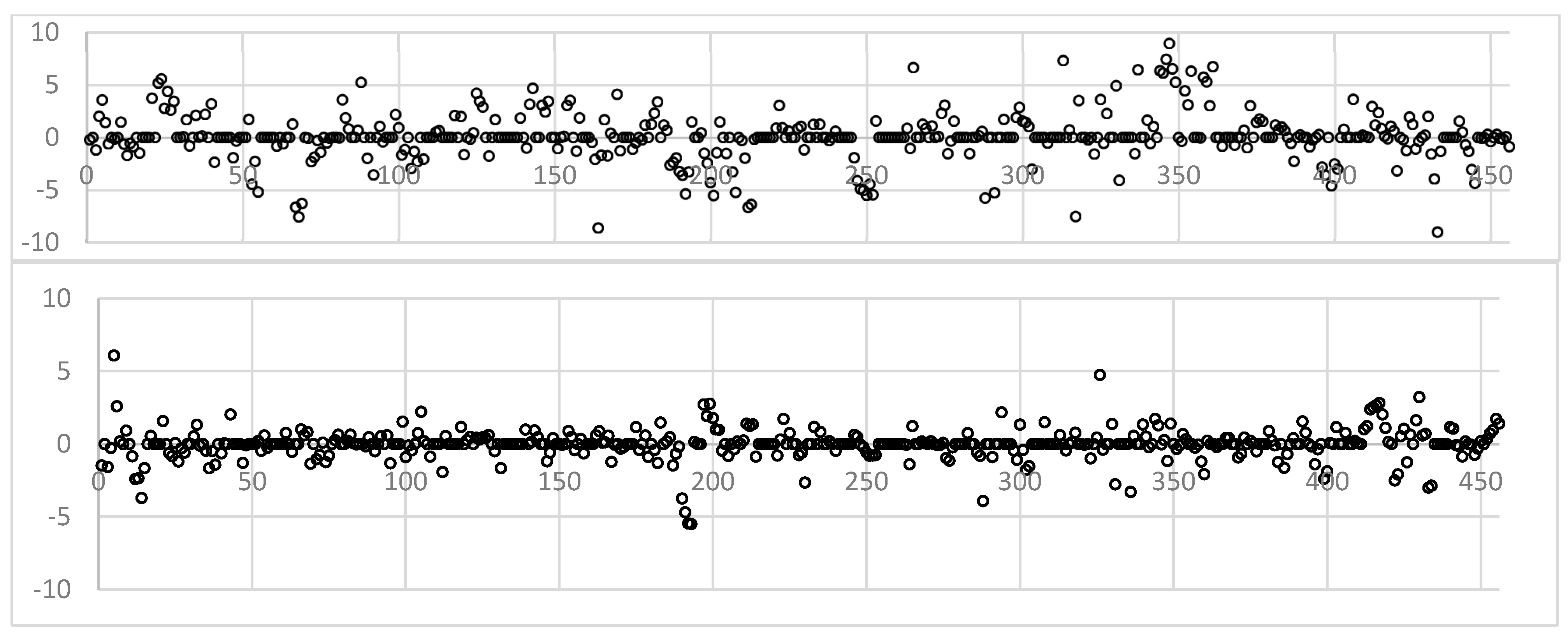
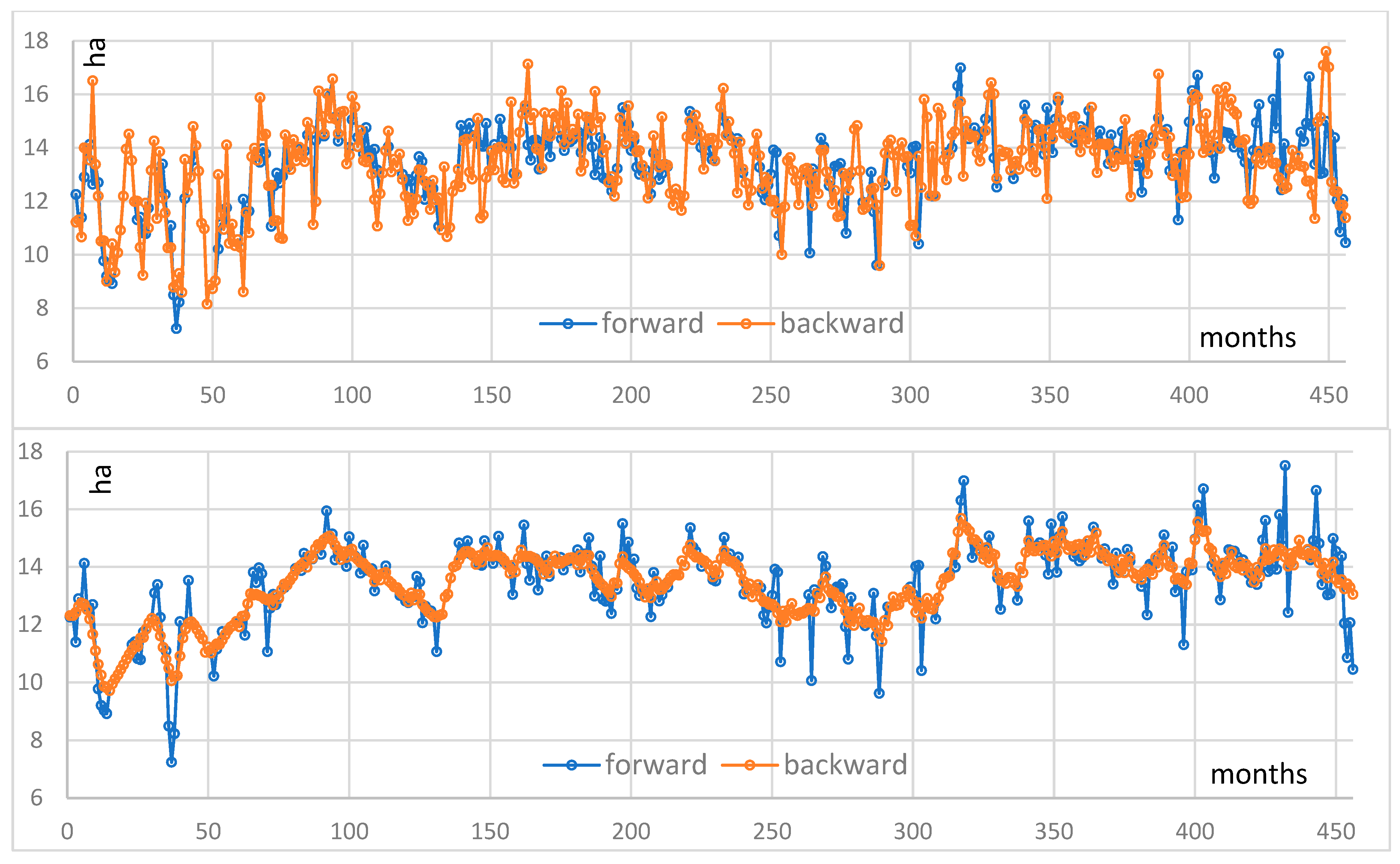
| Forward | Backward | Residual | Forward | Backward | Residual | |
| Number of data [n]: | 456 | 456 | 456 | 456 | 456 | 456 |
| Minimum: | 0.080 | 0.910 | –9.01 | 0.080 | –1.32 | –5.50 |
| Maximum: | 37.3 | 39.2 | 8.95 | 34.2 | 33.0 | 6.08 |
| Average: | 22.4 | 22.3 | 0.0633 | 22.4 | 22.4 | –0.0122 |
| Standard deviation: | 6.36 | 6.19 | 2.27 | 6.09 | 5.97 | 1.06 |
| Median: | 23.6 | 23.0 | 0.00 | 23.7 | 23.6 | 0.00 |
| Coefficient of variation [Cv]: | 0.284 | 0.277 | 35.8 | 0.272 | 0.267 | –86.9 |
| Skewness coefficient [Cs]: | –1.37 | –1.21 | –0.113 | –1.61 | –1.74 | –0.449 |
| Kurtosis coefficient [Ck]: | 5.74 | 5.87 | 6.13 | 6.32 | 6.93 | 10.8 |
| R—Interpolation | K—Interpolation | |||||
|---|---|---|---|---|---|---|
| Forward | Backward | Residual | Forward | Backward | Residual | |
| Number of data [n]: | 456 | 456 | 456 | 456 | 456 | 456 |
| Minimum: | 7.24 | 8.15 | –4.01 | 7.24 | 9.72 | –2.81 |
| Maximum: | 17.5 | 17.6 | 4.64 | 17.5 | 15.7 | 3.18 |
| Average: | 13.4 | 13.4 | 0.0331 | 13.4 | 13.4 | –0.00947 |
| Standard deviation: | 1.55 | 1.61 | 1.02 | 1.38 | 1.15 | 0.585 |
| Median: | 13.8 | 13.6 | 0.00 | 13.7 | 13.7 | 0.00 |
| Coefficient of variation [Cv]: | 0.115 | 0.121 | 30.9 | 0.102 | 0.0855 | –61.7 |
| Skewness coefficient [Cs]: | –0.915 | –0.528 | 0.177 | –0.939 | –0.910 | –0.562 |
| Kurtosis coefficient [Ck]: | 4.34 | 3.44 | 6.24 | 4.78 | 3.49 | 9.60 |
| R—Interpolation | K—Interpolation | |||||
|---|---|---|---|---|---|---|
| Forward | Backward | Residual | Forward | Backward | Residual | |
| Number of data [n]: | 456 | 456 | 456 | 456 | 456 | 456 |
| Minimum: | 3.88 | 3.59 | –2.05 | 4.05 | 4.50 | –1.21 |
| Maximum: | 9.42 | 9.87 | 1.99 | 9.18 | 8.64 | 0.99 |
| Average: | 6.20 | 6.21 | –0.0129 | 6.13 | 6.14 | –0.0113 |
| Standard deviation: | 1.09 | 1.19 | 0.542 | 0.898 | 0.839 | 0.240 |
| Median: | 6.18 | 6.14 | 0.00 | 6.05 | 6.08 | 0.00 |
| Coefficient of variation [Cv]: | 0.175 | 0.192 | –42.0 | 0.147 | 0.137 | –21.3 |
| Skewness coefficient [Cs]: | 0.218 | 0.295 | –0.374 | 0.226 | 0.289 | –0.728 |
| Kurtosis coefficient [Ck]: | 2.56 | 2.67 | 5.90 | 2.52 | 2.36 | 9.58 |
Disclaimer/Publisher’s Note: The statements, opinions and data contained in all publications are solely those of the individual author(s) and contributor(s) and not of MDPI and/or the editor(s). MDPI and/or the editor(s) disclaim responsibility for any injury to people or property resulting from any ideas, methods, instructions or products referred to in the content. |
© 2024 by the authors. Licensee MDPI, Basel, Switzerland. This article is an open access article distributed under the terms and conditions of the Creative Commons Attribution (CC BY) license (https://creativecommons.org/licenses/by/4.0/).
Share and Cite
Haidu, I.; El Orfi, T.; Magyari-Sáska, Z.; Lebaut, S.; El Gachi, M. Modeling the Long-Term Variability in the Surfaces of Three Lakes in Morocco with Limited Remote Sensing Image Sources. Remote Sens. 2024, 16, 3133. https://doi.org/10.3390/rs16173133
Haidu I, El Orfi T, Magyari-Sáska Z, Lebaut S, El Gachi M. Modeling the Long-Term Variability in the Surfaces of Three Lakes in Morocco with Limited Remote Sensing Image Sources. Remote Sensing. 2024; 16(17):3133. https://doi.org/10.3390/rs16173133
Chicago/Turabian StyleHaidu, Ionel, Tarik El Orfi, Zsolt Magyari-Sáska, Sébastien Lebaut, and Mohamed El Gachi. 2024. "Modeling the Long-Term Variability in the Surfaces of Three Lakes in Morocco with Limited Remote Sensing Image Sources" Remote Sensing 16, no. 17: 3133. https://doi.org/10.3390/rs16173133