Abstract
Polarimetric high-resolution range profile (HRRP), with its rich polarimetric and spatial information, has become increasingly important in radar automatic target recognition (RATR). This study proposes an interpretable target-aware vision Transformer (ITAViT) for polarimetric HRRP target recognition with a novel attention loss. In ITAViT, we initially fuse the polarimetric features and the amplitude of polarimetric HRRP with a polarimetric preprocessing layer (PPL) to obtain the feature map as the input of the subsequent network. The vision Transformer (ViT) is then used as the backbone to automatically extract both local and global features. Most importantly, we introduce a novel attention loss to optimize the alignment between the attention map and the HRRP span. Thus, it can improve the difference between the target and the background, and enable the model to more effectively focus on real target areas. Experiments on a simulated X-band dataset demonstrate that our proposed ITAViT outperforms comparative models under various experimental conditions. Ablation studies highlight the effectiveness of polarimetric preprocessing and attention loss. Furthermore, the visualization of the self-attention mechanism suggests that attention loss enhances the interpretability of the network.
1. Introduction
Radar automatic target recognition (RATR) represents a pivotal advancement in military and civilian radar systems, enabling the extraction and analysis of specific features from radar echoes [1,2,3]. This process allows for the automatic recognition of targets based on their attributes, beyond merely tracking their speed and location. The adoption of RATR transforms radar systems from simple detection tools into integral components of advanced intelligence and reconnaissance frameworks, marking a significant leap toward fully autonomous and intelligent defense systems.
Methods for RATR can be primarily divided into two types: those based on narrow-band and wide-band radar systems. Using narrow-band information for RATR involves analyzing data with a limited frequency range, such as radar cross section (RCS) sequences [4,5,6] and Doppler or micro-Doppler signatures [7,8,9]. These methods have the advantage of requiring less data, which simplifies collection and enhances processing efficiency. However, since the target size is usually smaller than the resolution of narrow-band radar, RATR methods based on narrow-band radar often struggle to obtain detailed target information, which in turn, limits the recognition rate. Wide-band radar systems, such as synthetic aperture radar (SAR) [10,11,12] and inverse synthetic aperture radar (ISAR) [13,14,15], use wide-band signals to easily obtain more detailed target recognition. The wide-band-based methods can improve recognition performance with rich detailed information about the target. However, the significant data size and complex imaging algorithms pose severe challenges in data handling and real-time processing. Thus, the efficiency of SAR and ISAR is constrained by their operational demands. A high-resolution range profile (HRRP) represents the projection of a target on the line of sight. It provides more detailed target information than RCS. Compared to SAR and ISAR images, HRRP is easier to store and process. Thus, HRRP-based RATR has received widespread attention.
Currently, HRRP-based RATR methods can be roughly categorized into two types: traditional methods [16,17,18] and deep learning methods [19,20,21]. Li et al. [22] first introduced a framework for HRRP-based RATR, encompassing data collection, preprocessing, feature extraction, and classifier design. Subsequent research has mainly concentrated on feature extraction, which can be divided into two main strategies: dimensionality reduction and data transformation. The dimensionality reduction approach reduces the volume of HRRP data using subspace or sparse methods [23,24]. The data transformation approach converts HRRP into frequency domain representations, such as bi-spectrum or spectrogram [25,26]. Although the features extracted by these methods are highly interpretable, their dependence on experience and inconsistent performance across different datasets constrain their applicability in real-world scenarios.
In recent years, deep learning methods have been widely used in HRRP-based RATR, which can be broadly categorized into three main types. The first type involves auto-encoder models, which leverage signal reconstruction to extract data features for recognition. Pan et al. [27] developed an innovative HRRP target recognition approach utilizing discriminative deep auto-encoders to boost classification accuracy with a limited number of training samples. Du et al. [28] presented a factorized discriminative conditional variational auto-encoder designed to extract features resilient to variations in target orientation. Zhang et al. [29] proposed a patch-wise auto-encoder based on transformers (PwAET) to enhance performance under different noise conditions. These auto-encoder-based methods exhibit strong noise reduction abilities. However, the limited feature extraction capabilities and the requirement for high similarity between training and testing samples restrict their generalization ability.
The second type of method utilizes convolutional neural networks (CNNs), which enable the automatic extraction of local features from HRRP. Wan et al. [30] employed a one-dimensional CNN for processing HRRP in the time domain and a two-dimensional CNN for spectrogram features. Fu et al. [31] applied a residual CNN architecture for ship target recognition. Chen et al. [32] introduced a target-attentional convolutional neural network (TACNN) to improve target recognition effectiveness. Although CNNs are effective in image processing, they struggle to extract global features due to their restricted receptive fields.
For the last type, time-sequential models, including recurrent neural networks (RNNs), long short-term memory networks (LSTMs), and Transformers, are employed to capture temporal features between different range cells. In 2019, Xu et al. [33] introduced a target-aware recurrent attentional network (TARAN) to exploit temporal dependencies and highlight informative regions in HRRP. Zhang et al. [34] proposed a deep model combining a convolutional long short-term memory (ConvLSTM) network with a self-attention mechanism for polarimetric HRRP target recognition. Pan et al. [35] designed a stacked CNN–Bi-RNN with an attention mechanism (SCRAM) to enhance generalization in scenarios with limited samples. In 2022, Diao et al. [36] pioneered the application of the Transformer for HRRP target recognition. These time-sequential models treat HRRP as sequential data. However, HRRP reflects the scattering distribution, so it is more appropriate to consider it as a one-dimensional profile rather than sequential data. Consequently, time-sequential models may overlook the spatial features of targets presented within HRRP.
Currently, most research focuses on extracting the spatial features of HRRP, with few scholars paying attention to the polarimetric features of HRRP. Polarimetric radars work by transmitting and receiving electromagnetic waves in various polarimetric states, significantly enhancing the radar’s capability to obtain more information about the target’s structure. Polarimetric HRRP integrates the advantages of polarimetric radars and wide-band radars, thereby improving the accuracy and reliability of RATR systems. Long et al. [37] applied decomposition along the slow time dimension in a dual polarimetric HRRP sequence and designed a six-zone plane for classification. This is a traditional method of using polarimetric features for classification. Some studies have also integrated polarimetric information into deep networks. For instance, in [38], the amplitude of different polarization channels was used for dual-band polarimetric HRRP target recognition, but this approach might lose the rich phase information present in polarimetric HRRP. Zhang et al. used amplitude and phase features in [34], and in [39], they utilized the real and imaginary parts of polarimetric HRRP and extracted artificial features to guide the model classification. However, experiments have shown that phase, real, and imaginary parts are unstable and not conducive to network learning. Therefore, new methods need to be explored to fully utilize polarimetric information in deep learning networks.
HRRP is often sparse, containing not only scattering information from the target but also from non-target areas. The majority of approaches treat these areas without distinction, hindering the effective use of the most critical range cells in HRRP. One method is to detect the target in the HRRP and then recognize it [40]. However, this method increases complexity, and the recognition result is greatly affected by the performance of the previous detection algorithm, leading to inevitable information loss. Additionally, the target area still includes some undesirable information that may degrade the identification, and the detection method cannot remove them. The self-attention mechanism offers another solution, thanks to its ability to identify and emphasize crucial parts of the input data [29,32,33,34,35]. However, the practicality of this mechanism is limited by the requirement of extensive datasets and an effective training process. Furthermore, these methods often lack good generalization and interpretability.
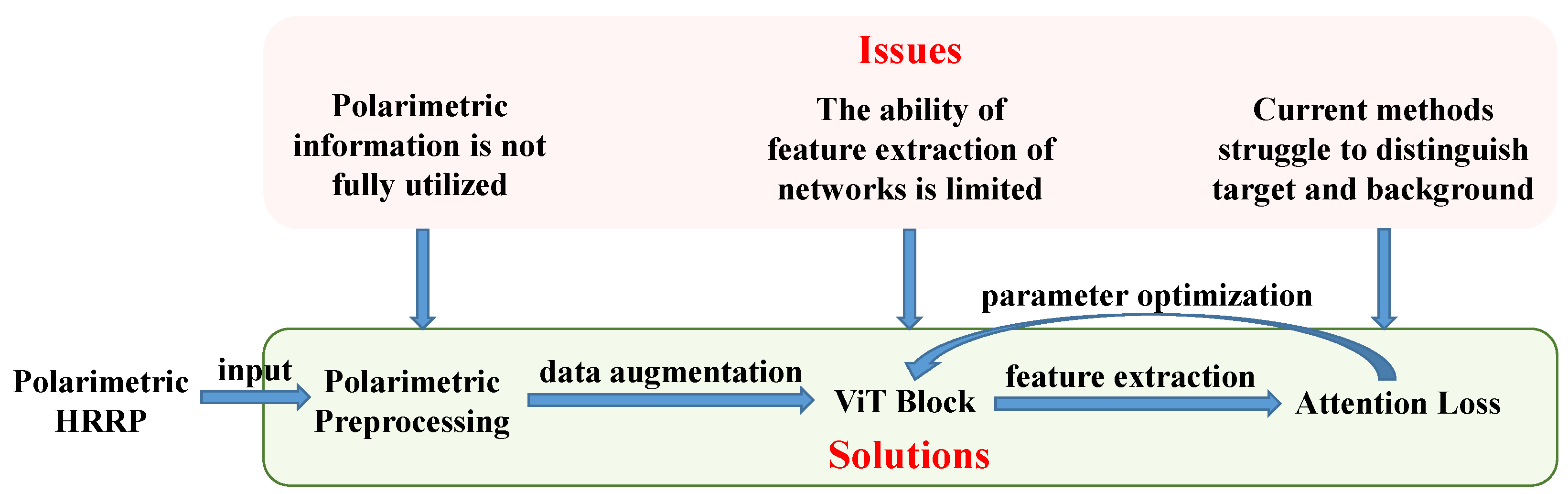
In summary, current HRRP-based RATR methods face three main issues. First, the feature extraction capabilities of the networks are limited. To address this, we use the vision Transformer (ViT) [41] as the backbone network. This model is a variant of the Transformer [42] in the field of image processing. It outperforms auto-encoders in feature extraction, provides a more comprehensive view of global features than CNNs, and better captures the image details of HRRP than traditional time-sequential models, such as RNNs and LSTMs. Second, polarimetric information has not been fully utilized, especially in deep learning methods. To tackle this, we perform two coherent and two incoherent polarimetric decomposition methods. Inspired by [43], we use one-dimensional convolution to increase the number of channels of polarimetric information, which enhances the network’s performance. Last but not least, current methods struggle to distinguish between target and non-target areas in HRRP, resulting in poor generalization and interpretability. In previous studies, attention maps have predominantly been utilized to observe the effects of network training [29,36,39], but they have not been leveraged to enhance network performance. We propose to integrate the difference between the attention map and HRRP span into the loss function to steer the network to focus on range cells of real targets. We previously introduced the foundational ideas in [44]. In this paper, we significantly extend that work by providing a more comprehensive background analysis, incorporating additional polarimetric preprocessing techniques, detailing the attention loss function and its back-propagation process, and conducting extensive supplementary experiments. These expansions not only demonstrate the effectiveness of our proposed method under various conditions but also offer deeper insights into the model’s performance and generalization capabilities. In more detail, this paper makes the main contributions as follows:
- To the best of our knowledge, this paper is the first to apply ViT to polarimetric HRRP target recognition. Experimental results show that our ViT-based method ITAViT consistently outperforms existing approaches across various conditions, achieving superior recognition performance. Furthermore, compared to its base model, the Transformer, ViT provides significant advantages in both recognition accuracy and computational efficiency.
- We propose a hybrid approach that combines traditional feature extraction with a polarimetric preprocessing layer (PPL) to optimize the utilization of polarimetric information, integrating the strengths of both traditional methods and CNNs. Through ablation experiments, we analyze the performance of different features and find that combining the amplitude of polarimetric HRRP with coherent polarimetric features achieves the best performance. We also demonstrate the effectiveness of PPL through comparative experiments.
- A novel attention loss is constructed to guide the model to focus on range cells of real HRRP targets during training and inference processes, and its back-propagation process is derived. This method does not require modifications to the internal structure of the network and much additional computational overhead. The effectiveness of attention loss is demonstrated under various experimental conditions, including scenarios with noise and clutter, as well as situations where there are significant differences between the training and test sets. The results highlight the robustness and generalization capabilities of our proposed method. Additionally, the attention loss offers improved interpretability of the self-attention-based HRRP target recognition task through the visualization of the attention map.
In Figure 1, we present a high-level block diagram of the proposed method to explain the relationship between our contributions and the identified issues, and to illustrate the connections between different modules.
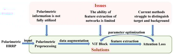
Figure 1.
A high-level block diagram of the proposed method.
The remainder of this paper is organized as follows. In Section 2, we describe the representation of polarimetric HRRP and introduce our proposed method, ITAViT. Section 3 describes the experimental data and presents the experimental results as well as comparisons with other methods. Section 4 analyzes the roles of the three components of the network separately. Finally, Section 5 concludes the paper.
2. Method
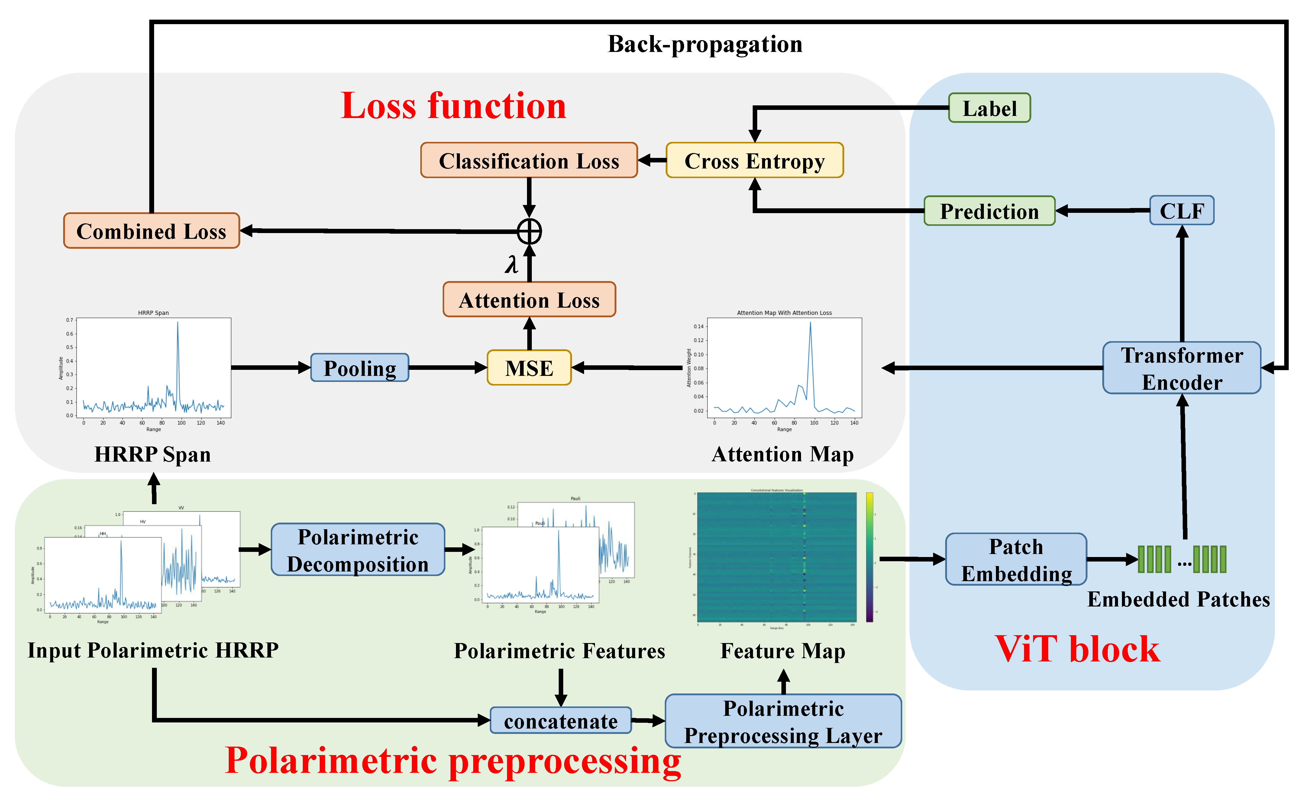
An overview of our proposed method, ITAViT, is illustrated in Figure 2. The entire network primarily consists of three components: polarimetric preprocessing, the ViT block, and the loss function. In the polarimetric preprocessing stage, we concatenate the polarimetric features obtained from polarimetric decomposition with the amplitude of the input polarimetric HRRP. These combined data are then fed into the PPL to generate a fusion feature map, which is subsequently input into the ViT block. Within the block, the feature map is transformed into embedded patches through patch embedding and then processed by the Transformer encoder. The encoder, via a classification head (CLF), generates the prediction and also produces an attention map indicating the attention level of different patches. For the loss function calculation, the prediction and the real label are used to compute the classification loss via cross-entropy. Simultaneously, the attention loss between the attention map and the pooled HRRP span is computed via mean square error (MSE) during the training process. The total loss is the combination of these two components.
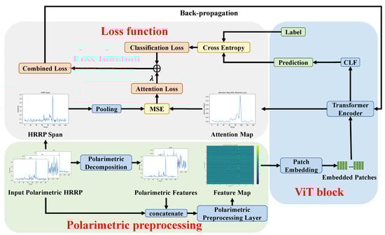
Figure 2.
An overview of the proposed method ITAViT.
2.1. Representation of Polarimetric HRRP
Linear frequency modulated signals are widely used in high-resolution imaging, and the signal can be expressed as [45]:
where t is the fast time variable, T is the pulse duration, is the slope of frequency modulation, is the central frequency of the transmitted signal. is a rectangular window function. According to the scattering center model [46], in high-frequency situations where the target size is larger than the radar’s range resolution, the target echo can be approximated as the sum of the echoes from several strong scattering points on the target. Assuming the target has N scattering points, the echo signal is given by:
where is the delay of the kth scattering point, is the distance between the scattering point and the radar, and is the amplitude of the signal reflected by the scattering point. After down-conversion to baseband and range compression, the received signal can be presented as [47]:
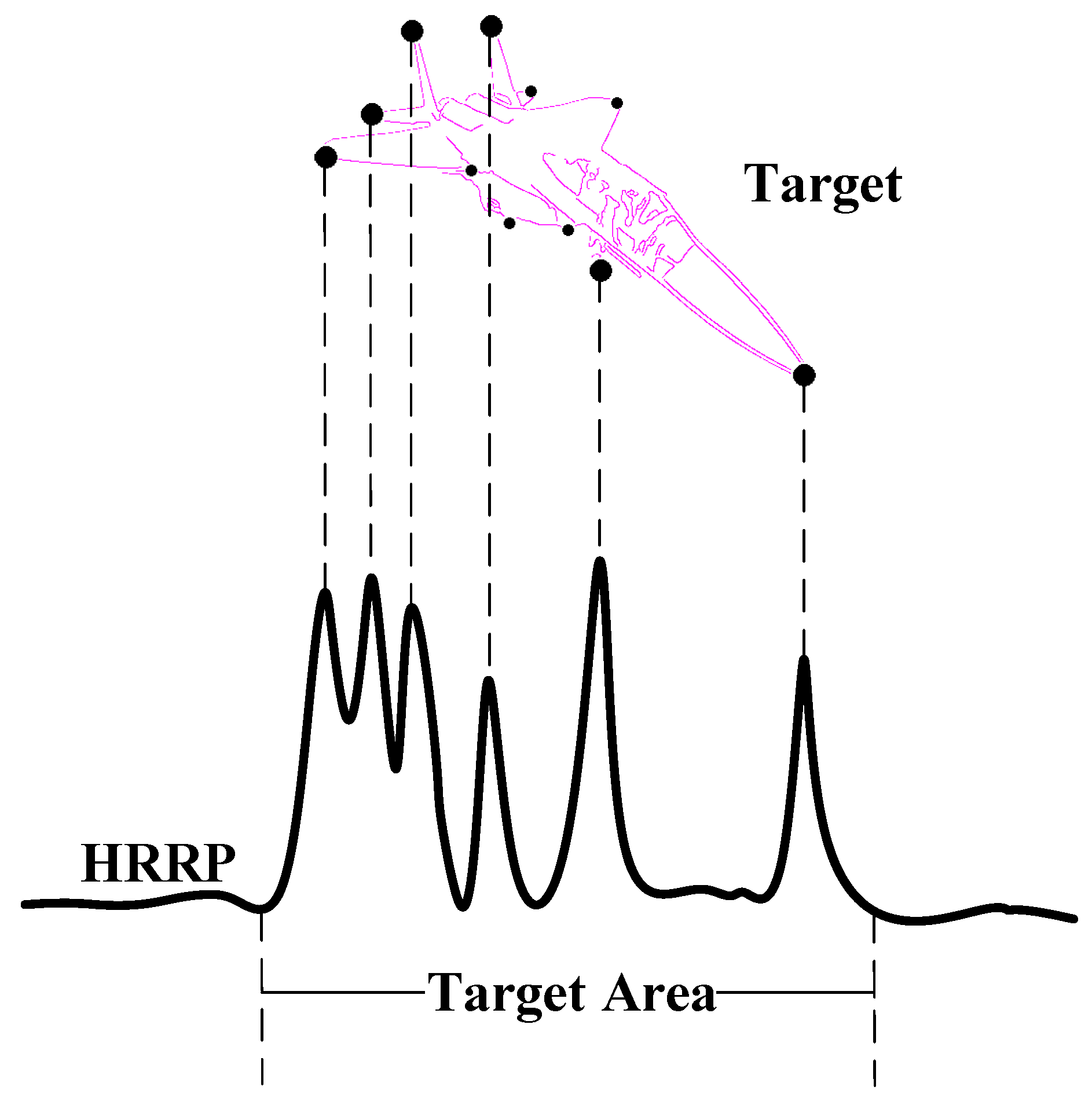
Here, is the amplitude of the kth scattering point in the compressed signal, is the bandwidth and is the wavelength. By sampling the fast time and converting the relationship between time and distance [47], the independent variable of the received signal can be transformed into range cells, thereby obtaining the HRRP. From this equation, we can observe that in HRRP, the scattering points appear in the form of sinc functions, manifesting as peaks. These peaks typically correspond to sharp regions of the target, which are crucial in RATR. Examples of such regions include the nose, wings, and tail of an airplane, as shown in Figure 3.

Figure 3.
The relationship between target and HRRP, where the dots on the target represent scattering points.
Polarimetric radars operate by transmitting and receiving electromagnetic waves in various polarimetric states. This polarimetric diversity significantly enhances the radar’s capability to obtain more information about the target’s structure. Unlike single-polarization radars, which can only observe a single channel complex value, polarimetric radars can obtain a complex scattering matrix in each range cell.
where represents the scattering coefficient when the receiving polarization and transmitting polarization are p and q, respectively, with . Here, denotes horizontal polarization, and denotes vertical polarization. In the monostatic backscattering case, where the transmitting and receiving antennas are colocated, we have . Thus, the polarimetric HRRP can be expressed as:
where L is the length of each HRRP sample and represents the data in one range cell. By summing the power of each range cell according to (6), we can obtain the HRRP span , which represents the overall shape of the polarimetric HRRP.
2.2. Polarimetric Preprocessing
We extract four manual polarimetric features from , including two coherent decomposition methods: Pauli decomposition and Krogager decomposition, and two incoherent decomposition methods: Cloude–Pottier decomposition and Freeman–Durden decomposition [48]. The primary difference between these two types of decomposition methods is that coherent decomposition decomposes the scattering matrix, while incoherent decomposition decomposes the coherency matrix. The coherency matrix can be obtained by averaging the Pauli vectors of several adjacent cells as follows.
where denotes the average over adjacent range cells and represents the Pauli vector, which can be calculated from .
We concatenate the extracted features based on the polarimetric decomposition with the amplitude of after normalization, resulting in enhanced polarimetric HRRP data . Here, L is the number of range cells in a sample, and is the dimension of the extracted features (e.g., for Krogager decomposition). We add 3 to because includes three channels, i.e., HH, VV, and HV. We normalize each HRRP sample by dividing all values by the maximum amplitude within that sample. It is necessary because HRRP is amplitude-sensitive, meaning that even for the same target and radar, the amplitude can vary due to factors such as target distance and environmental conditions, leading to inconsistencies in scale. To address this, it is standard practice to discard the intensity information and focus on the shape of the HRRP, which is effectively achieved through normalization. The extracted features also need to be normalized individually, except for the Cloude–Pottier features, as they inherently reside within a fixed dynamic range and have well-defined numerical significance. Normalizing these features could distort their original meaning. is then fed into the PPL. In this layer, inspired by [43], we use one-dimensional convolution to increase the number of channels of polarimetric information. The output feature map is denoted as , where D is the number of channels output by the PPL. By concatenating the amplitude and manual polarimetric features and using PPL, we can combine the advantages of traditional methods and deep learning approaches. This not only enhances the overall interpretability of the model but also fully utilizes the polarimetric features.
2.3. ViT Block
To facilitate understanding, the data transformation process within the ViT block and the calculation workflows for the loss function are clearly illustrated in Figure 4.
Figure 4.
The data flow diagram in ViT block and the calculation workflows for the loss function.
The ViT block [41] is the core component of the entire network. Unlike the process in a Transformer, where the sequence is directly fed into the encoder, in ViT we first segment the preprocessed feature map into patches, transforming from to . Here, P represents the length of each patch. These patches are then fed into a fully connected layer for patch embedding, resulting in embedded patches with the size of , where is the number of patches and is the hidden dimension. To incorporate positional information and ensure that the model is aware of the spatial order of the patches, a positional encoding is added to before feeding it into the Transformer encoder. Similar to the approach used in ViT [41], we use learnable positional encoding in our implementation, where a parameter matrix is initialized and learned during the training process. The embedded patches are then fed into the Transformer encoder, where the core component is the self-attention mechanism, which computes the attention scores based on the queries (), keys (), and values () [42].
where , and are different learned weight matrices. The attention scores are calculated using the scaled dot-product attention, which is defined as:
where represents the dimension of the key vectors. This mechanism allows the model to focus on different parts of the input sequences, weighting them according to their importance.
The Transformer encoder utilizes a multi-head self-attention (MSA) mechanism to enhance its capability, allowing for the parallel processing of information across various representational subspaces. Each attention head independently projects , and , then calculates attention weights and outputs accordingly. The outputs from all heads are subsequently concatenated and transformed by a final projection matrix to yield the composite multi-head attention output.
, and are projection matrices in .
To facilitate subsequent calculations, we need to define some intermediate variables. Through the data transformation process, an attention matrix is obtained in , delineating the interrelations among different patches within the sequence. Concatenating the from the H heads results in the matrix .
where
We also define as the concatenation of from each head.
By averaging the attention matrices from each head, an aggregate matrix is obtained as shown in (16). In this matrix, each element signifies the average attention received by the jth patch from the ith patch.
where
in which is the identity matrix.
To determine the overall significance of each patch, we examine the mean attention value it receives from all other patches. This is achieved by averaging each column of as shown in (18), thereby assigning each patch a singular attention score, reflecting its average importance across the entire sequence. This importance vector is denoted as and is used to calculate the attention loss introduced in the next subsection.
where is a vector of ones.
2.4. Loss Function
2.4.1. The Calculation Process
In our proposed method, the loss function is composed of two parts: the classification loss and the attention loss. The output of the MSA is passed through a series of feed-forward neural networks and is then fed into a fully connected layer to obtain the predicted classification labels, denoted as . The prediction is combined with the label y to calculate the classification loss using cross-entropy [32].
where is the number of classes.
To further enhance the model’s performance, we propose a novel attention loss. A key difference between HRRP and optical images is that the amplitude of HRRP carries specific prior information. In optical images, segregating targets from the background simply based on pixel values is challenging. In ViT, a large dataset and extensive training time are typically necessary for the self-attention mechanism to identify target regions. However, in HRRP, range cells with higher amplitude correspond to stronger scattering points of the target, thereby containing richer information that is beneficial for distinguishing between different categories of targets. We aim to leverage this prior knowledge to reduce the influence of noise and non-target areas on classification.
Based on this phenomenon, we develop the attention loss to guide the network to focus on those range cells with higher intensity. Since the peaks in the HRRP span represent important scattering points for RATR, and the attention map illustrates the importance of each patch, we introduce attention loss to optimize the attention map, i.e., , making it more similar to the HRRP span, i.e., . This guides the network to focus on target regions and reduce the influence of non-target regions. After patch embedding, the length of is equal to the number of patches, while the length of is equal to the number of range cells. Additionally, is a row vector because it is obtained by averaging the columns of as shown in (18), whereas is a column vector. To align with , we transpose and pool it with a down-sampling factor equal to the patch size. To ensure that represents the degree of importance, we also normalize . Then, the MSE is used to quantify the distance between and , thus deriving the attention loss.
The total loss is the combination of the classification loss and the attention loss.
where is the weighting factor used to balance the two components of the loss function. We need to point out that this parameter needs to be adjusted according to the specific dataset being used. If is set too high, the network might focus excessively on attention loss, which could lead it away from the primary task of target recognition. Conversely, if is too low, the attention loss may become ineffective.
2.4.2. The Back-Propagation Process of Attention Loss
From Figure 4, we can see that is related to all parameter matrices within the encoder, thus allowing for the optimization of the entire network during the back-propagation process. In contrast, does not directly optimize the network’s output. It only influences the network parameters and by optimizing the attention map, thereby playing a role in the network’s training. Since classification loss has been widely used, we specifically derive the back-propagation process of our proposed attention loss.
Expanding (20) into the form of a vector inner product, we obtain:
Furthermore, the differential of can be derived, leading to:
According to (18), the differential of can be written as:
Combining (23) and (24), we obtain (25).
The operator ⊙ represents element-wise product and the definition of and can be found in [49]. According to matrix differential theory, the partial derivative of to can be obtained as (26). Note, that the transpose of can be omitted because is a symmetric matrix.
After a similar calculation as [49], we obtain the partial derivative of with respect to and as follows:
where has an identity matrix in the ith column, while other entries are zero matrices.
3. Result
3.1. Dataset and Experiment Settings
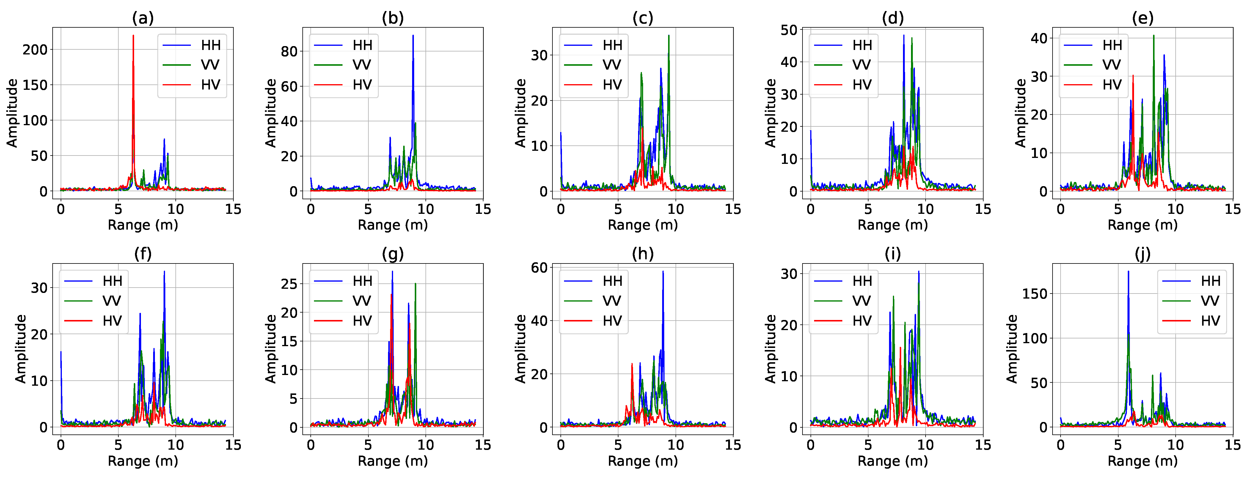
An overview of the experimental dataset is shown in Table 1. The experimental results are based on a dataset of simulated X-band signatures of civilian vehicles released by the Air Force Research laboratory [50]. To the best of our knowledge, this is the only publicly available dataset for polarimetric HRRP target recognition. The dataset consists of ten types of civilian vehicles: Camry, Civic 4dr, Jeep93, Jeep99, Maxima, MPV, Mitsubishi, Sentra, Avalon, and Tacoma. The simulated radar operates at a central frequency of 9.6 GHz with a bandwidth of 1.5 GHz. Polarimetric HRRP data are generated at four different pitch angles: , , , and . Samples of the simulated polarimetric HRRP are presented in Figure 5. The radar azimuth angle ranges from to in increments of . Thus, a polarimetric HRRP dataset of = 14,400 samples is obtained.

Table 1.
Dataset Overview.
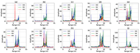
Figure 5.
Ten samples in simulated polarimetric HRRP dataset. (a) Camry (b) Civic 4dr (c) Jeep93 (d) Jeep99 (e) Maxima (f) MPV (g) Mitsubishi (h) Sentra (i) Avalon (j) Tacoma.
We use two methods to partition the dataset to evaluate the model’s performance: the standard operating condition (SOC), where the training and test sets have similar observation conditions, and the extended operating condition (EOC), where there are significant differences between the training and test sets on observation conditions. Specifically, in SOC the dataset is randomly divided with an 8:2 ratio, where 80% of the data are used for training and the remaining 20% are used for testing. In EOC, we organize the training and test sets by selecting HRRPs with pitch angles of , , and for training, and HRRPs with a pitch angle of for testing. These two partitioning methods are used to specifically verify the robustness and generalization of our proposed method.
Our network is implemented using PyTorch 1.11.0 in combination with Huggingface. The configurations and parameter settings of the proposed model, as shown in Table 2, represent the optimal combination obtained through grid search. The experiments are conducted on an NVIDIA GeForce RTX 3090 GPU with a memory of 24 GB. The balancing factor for the loss function, i.e., , is set to 100. We optimize the model using the Adam optimizer with a learning rate of 0.0005, and the network is trained for a total of 2000 epochs. We use a small learning rate because our dataset is relatively small. If we choose a larger learning rate, it may lead to overfitting. To minimize the impact of random errors, each experiment in this paper is repeated 10 times, and the average results are reported. Noise is added to the HRRP at different signal-to-noise ratios (SNRs). The definition of SNR is the same as [35]:
where denotes the power of HRRP data in the lth range cell, L is the total number of range cells and denotes the power of noise.
Table 2.
Configurations and Parameter Settings of the Proposed Model.
3.2. Model Recognition Accuracy Performance
3.2.1. Recognition Results
At the SNR of 20 dB, the confusion matrix of the proposed method is shown in Table 3, which reveals that the classification accuracy for most categories exceeds 94%, with Tacoma achieving an impressive 100% accuracy. The results indicate a highly effective classification performance.
Table 3.
The confusion matrix of the proposed method in SOC (Percentage).
The results from feature visualization align with those from the confusion matrix. We employ t-distributed stochastic neighbor embedding (t-SNE) [51] to reduce the dimension of the features before the fully connected classification layer down to two, which we then visualize in Figure 6. In this visualization, points of different colors represent different categories of vehicles. The features of the Tacoma are notably distant from those of other categories, accounting for its high classification accuracy. Correspondingly, categories that exhibit higher misclassification probabilities in the confusion matrix appear closer in the visualization, such as the Jeep93 and the Avalon.
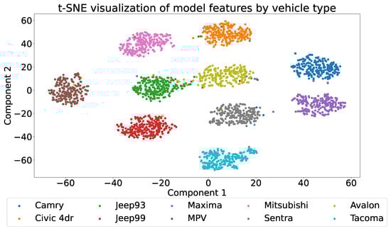
Figure 6.
Two-dimensional t-SNE projection of the extracted features.
3.2.2. Comparison with the Performance of Other Models
We compare our method in both SOC and EOC with other methods used for HRRP target recognition and consider the average recognition rate across both conditions. The results are shown in Table 4. The comparison methods include traditional machine learning classification methods such as GMM, LDA, and SVM, as well as classical deep learning methods like 1-D CNN and 1-D RNN. We also include advanced models that integrate self-attention mechanisms, such as TACNN [32], TARAN [33], SCRAM [35], ConvLSTM [34] and PwAET [29]. To ensure fairness, the parameters for these comparative methods are determined through a grid search around the hyperparameters provided in the original papers, and the results obtained under the configurations that yield the highest recognition rates are used for comparison. The data presented in the table are the average results of ten repeated experiments. The comparison results show that our proposed method ITAViT achieves the best performance in terms of SOC (95.83%) and average recognition rates (69.23%) and also outperforms most comparison methods in EOC, demonstrating the effectiveness of our approach.
Table 4.
Recognition accuracy of different methods under SOC and EOC. The average accuracy of the two conditions is shown in the rightmost column.
Compared to traditional machine learning classification methods (groups 1–3), deep learning methods (groups 4–11) significantly improve recognition rates under both SOC and EOC. Group 4 (1D-CNN) shows slightly better recognition performance than Group 5 (1D-RNN), with average accuracies of 66.18% and 65.01%, respectively, indicating that HRRP is better treated as a one-dimensional profile rather than a time sequence. Introducing the self-attention mechanism, although the recognition rates in SOC for groups 6–9 do not significantly improve compared to groups 4–5, there is still a notable improvement in EOC recognition rates, all exceeding 40%. Among them, groups 7 and 8 achieve the highest EOC recognition rates at 43.46% and 43.09%, respectively, suggesting that the self-attention mechanism helps the model focus on critical areas for recognition, thus maintaining good generalization performance even when there is a significant difference between the training and test sets under EOC. With accuracies of 95.83% and 93.56% under SOC, our proposed method (group 11) and PwAET (group 10) outperform other deep learning models, highlighting the excellent feature extraction capabilities of ViT. Our method surpasses PwAET in EOC recognition rates, achieving 42.63% compared to 38.11% of PwAET, indicating that our proposed attention loss has a better capability to distinguish target regions from non-target regions, compared to the reconstruction error-based loss function used in PwAET. We also notice that PwAET performs the worst under EOC among the methods based on deep learning, which may be related to the poor generalization ability of the auto-encoder.
4. Discussion
We separately investigate the roles of the three key modules in ITAViT: polarimetric preprocessing, ViT block, and attention loss.
4.1. The Effect of Polarimetric Preprocessing
We conduct ablation experiments to study the effects of polarimetric preprocessing, including the use of polarimetric information methods from previous works, such as using only amplitude [38], amplitude and phase [34], real and imaginary parts and features [39]. Additionally, we test our proposed polarimetric preprocessing method: combining amplitude with two types of coherent decomposition features (Pauli and Krogager) and two types of incoherent decomposition features (Cloude–Pottier and Freeman–Durden), respectively. For each combination, we experiment with and without the PPL. The results are shown in Table 5.
Table 5.
Comparison of Recognition Accuracy in SOC with Different Polarimetric Features.
We can observe the following phenomena from Table 5. Using the combination of amplitude and coherent features (groups 6–8) achieves better recognition performance (ranging from 95.64% to 95.87%) compared to previous works that use polarimetric information (groups 1–3, ranging from 92.35% to 94.63%). Group 2 indicates that combining amplitude and phase interferes with the model’s recognition performance, achieving 92.35% without PPL. One reason is the periodic nature of phase information. For example, when phase angles are adjusted to a range of to , angles like and are correctly considered adjacent, but angles like and are numerically far apart despite being only apart. This discrepancy makes it difficult to effectively extract similar features. Additionally, the amplitude of the HV channel is much smaller than that of the HH and VV channels in most cases, which may lead to unstable phase information in the HV channel. Group 3 shows that using the real and imaginary parts combined with Pauli features (94.63%) is less effective than using amplitude combined with Pauli features (95.87%), likely due to the instability of the phase causing significant fluctuations in the real and imaginary parts.
The combination of amplitude and coherent features (groups 6 and 7) yields the best recognition performance (95.87% and 95.64%, respectively), especially compared to using only amplitude (group 1 at 94.54%). This demonstrates that polarimetric information effectively enhances HRRP classification performance. However, combining both coherent features and amplitude (group 8 at 95.69%) does not further improve recognition accuracy, indicating that simply stacking feature dimensions does not enhance recognition accuracy. The recognition accuracy using two types of incoherent features (groups 4 and 5 at 94.59% and 94.65%, respectively) does not show significant improvement compared to group 1 and is clearly inferior to coherent features. One possible reason for this issue is that the coherency matrix is computed by averaging over several adjacent range cells in incoherent features, as shown in (7). This averaging process reduces the range resolution of the HRRP, leading to a loss in the ability to distinguish closely spaced scattering points. Additionally, incoherent decomposition methods are generally modeled on the scattering characteristics of natural objects, which may not be applicable to man-made targets like vehicles.
Comparing the results of experiments with and without PPL, when using only amplitude information (group 1), the effect of PPL is not significant (94.54% with PPL compared to 94.26% without PPL). When phase information is added (group 2), using PPL significantly reduces recognition accuracy (87.70% with PPL compared to 92.35% without PPL) due to the increased instability caused by processing phase information with convolutional layers. This makes it harder for the network to learn meaningful features from the phase information. In the subsequent six groups of experiments, using PPL consistently outperforms not using it, with improvements ranging from 0.52% to 2.76%. This indicates that processing only amplitude information is relatively straightforward for the network, but after feature combination, PPL is needed to further extract potential polarimetric features, which helps the ViT block extract more efficient spatial features and increase classification accuracy.
In summary, while polarimetric information is indeed beneficial, it is crucial to extract the correct features and use appropriate processing methods. Our proposed method, which combines amplitude with coherent features and utilizes the PPL, has proven to be the most effective.
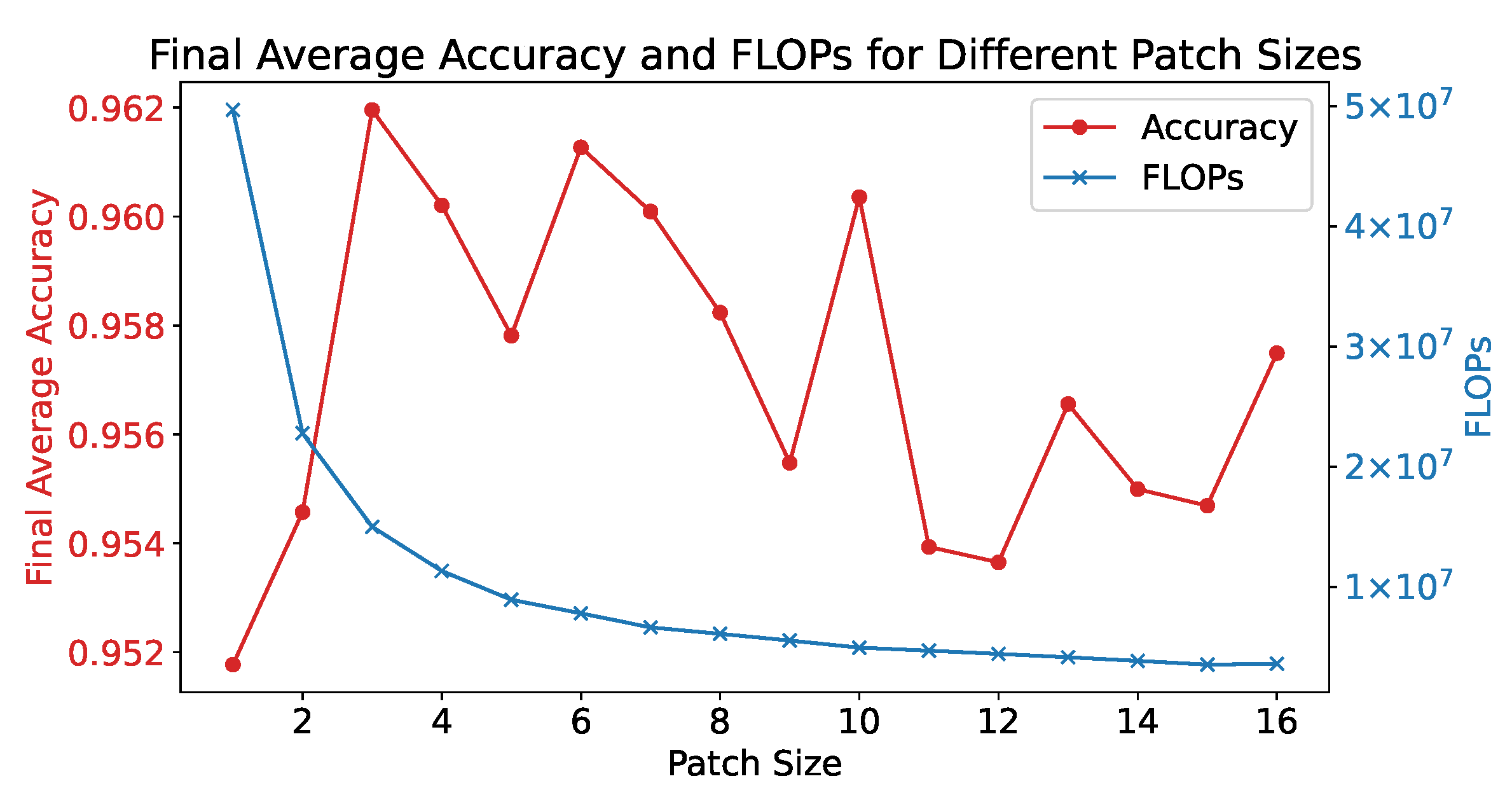
4.2. The Influence of Patch Size in ViT Block
We examine the effect of different patch sizes on the efficacy of our model from two key perspectives: recognition accuracy and computational complexity. The relationship between patch size, accuracy, and FLOPS (floating-point operations per second) is shown in Figure 7. With a patch size of 1, indicating no segmentation of HRRP data, ViT simplifies into a traditional Transformer architecture. This leads to an increased count of patches fed into the Transformer encoder, elevating both the computational and spatial complexity to a quadratic relation , with N being the number of patches. This directly contributes to a decrease in FLOPS with growing patch size, aligning with the trend represented by the blue line.
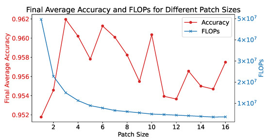
Figure 7.
The effect of different patch sizes. The accuracy curve is obtained by averaging the results of 10 repeated experiments.
A small patch size not only increases computational demand but also lowers recognition accuracy, as depicted by the red line. At a patch size of 1, accuracy is at its lowest, indicating that the network fails to extract local features from the data. This suggests that ViT is more suited for polarimetric HRRP classification than Transformer. Conversely, a larger patch size is not better, as it includes a large number of range cells within a single patch. This prevents the HRRP span from effectively highlighting the range cells with strong scattering points after pooling with a down-sampling factor equal to the patch size, because these range cells may be overshadowed by other weaker range cells within the same patch. Considering both computational burden and recognition accuracy, we select a patch size of 6 for our model.
4.3. The Effect of Attention Loss
4.3.1. Rationality Analysis of Attention Loss
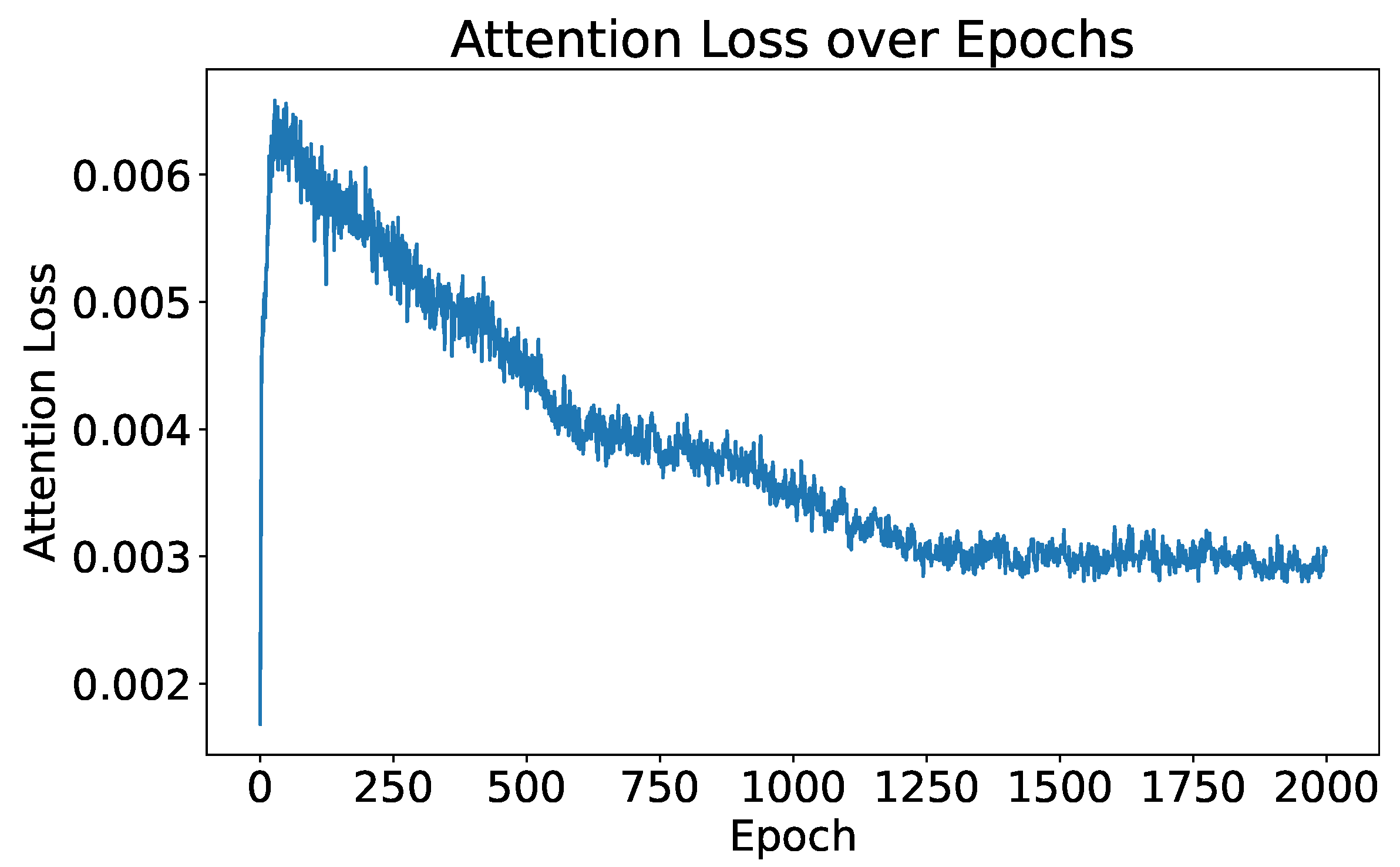
When attention loss is excluded from the optimization process by setting to zero, the trend of attention loss through the training process is illustrated in Figure 8. Initially, there is a notable increase in attention loss at the start of training. This is because, in the early stages of training, the network is focused solely on reducing the classification loss and has not yet stabilized. However, as the training stabilizes, attention loss decreases, indicating that the attention map increasingly resembles the HRRP span. This pattern suggests that even without optimizing the attention loss directly, the attention loss naturally decreases. This indicates that the network gradually aligns the attention map with the HRRP span, as the attention loss reflects their similarity. The purpose of optimizing attention loss is to speed up the network’s convergence and improve the model’s capability in identifying strong scattering points within the target, especially when the size of the training set is small and the training time is limited.
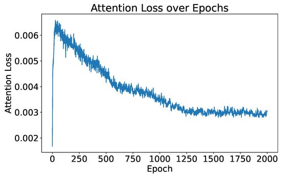
Figure 8.
Attention loss over epochs when only optimizing classification loss.
4.3.2. Performance under SOC
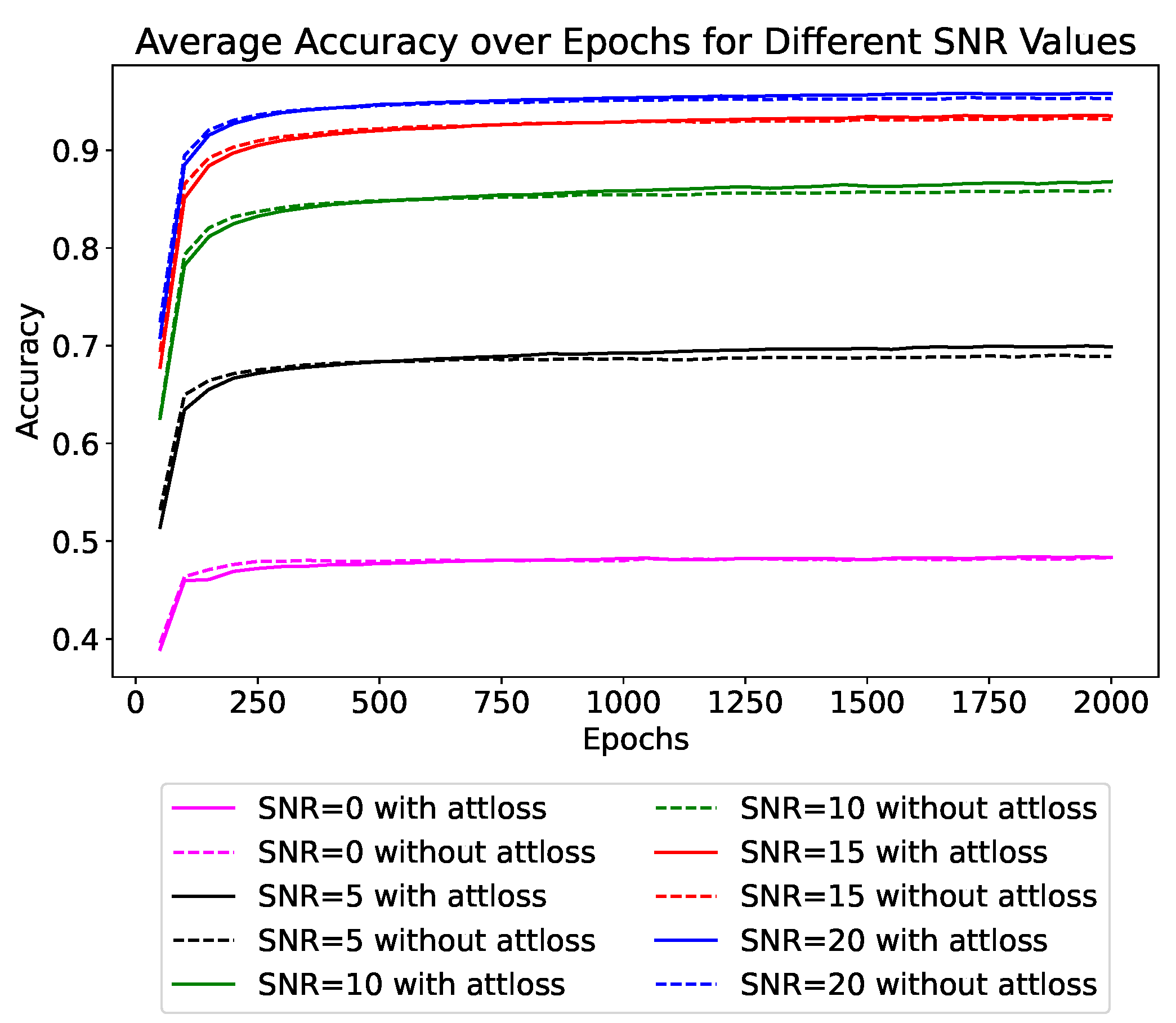
We specifically conduct ablation experiments to demonstrate the effectiveness of attention loss. We conduct experiments under different conditions: with SNR values of 0 dB, 5 dB, 10 dB, 15 dB, and 20 dB. In these experiments, we compare scenarios with and without the use of attention loss. The average accuracy results for each group of experiments are qualitatively illustrated in Figure 9. In the figure, different colors represent different SNR levels, and solid and dashed lines indicate experiments with and without attention loss, respectively. The final recognition rates are quantitatively presented in Table 6. The qualitative and quantitative experimental results clearly demonstrate that under each SNR condition, the classification accuracy with attention loss is higher than without it. This demonstrates that attention loss can enhance the network’s performance.
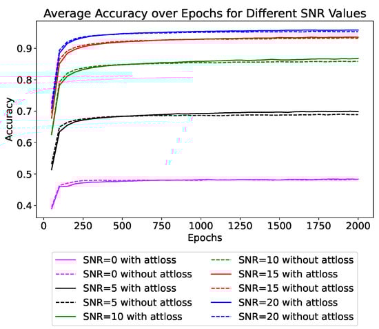
Figure 9.
The impact of attention loss on test accuracy in SOC. Different colors represent different SNRs, with solid and dashed lines indicating whether attention loss is used or not, respectively.
Table 6.
Accuracy at different SNR levels with and without attention loss in SOC.
Additionally, there are three noteworthy observations. Firstly, at the beginning of training, the dashed lines occasionally surpass the solid lines, seemingly indicating that the performance is better without the additional attention loss. This demonstrates that the initial large attention loss (as shown in Figure 8) can degrade the classification efficiency. However, with the increase in training epochs, the dashed line eventually falls below the solid line. This indicates that attention loss plays a positive role throughout the training process.
Secondly, the benefit of using attention loss is less pronounced when the noise level is low, with improvements of only 0.57% at 20 dB SNR and 0.39% at 15 dB SNR, but becomes more evident at lower SNRs, with improvements of 1.01% at 5 dB SNR and 0.93% at 10 dB SNR. Under significant noise influence, attention loss helps mitigate the impact of noise, allowing the model to focus more on the target’s characteristics. This enhances the network’s noise immunity and robustness. However, we find that at the SNR of 0 dB, attention loss almost fails, showing an improvement of only 0.01%. At this level, the signal and noise are of the same magnitude, making it difficult for attention loss to effectively focus on the target area, thus rendering it ineffective.
Finally, the dashed line essentially stops increasing after the midpoint of training, while the solid line continues to show an upward trend in the later stages of training. This indicates that incorporating attention loss can effectively improve the generalization capacity of the model.
4.3.3. Performance under EOC
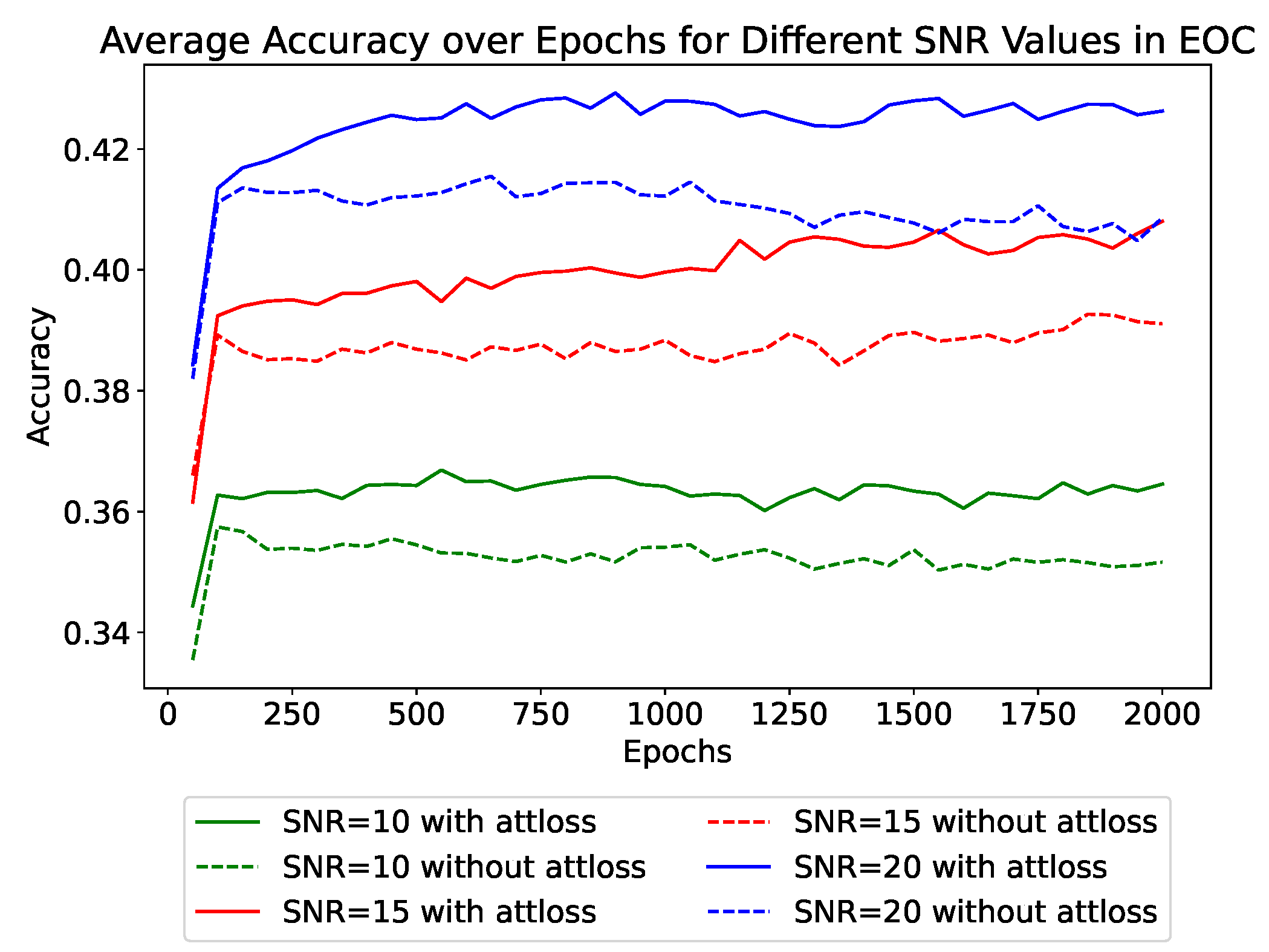
Compared to SOC, the recognition task under EOC is much more challenging. The challenge mainly comes from the distinct variation in observation angles between the training set and test set. Such variations influence the distribution and polarimetric characteristics of the target’s scattering points at different pitch angles. Similarly, we compare the recognition accuracy of models with and without attention loss under different SNR levels, as shown in Figure 10 and Table 7.
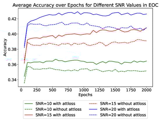
Figure 10.
The impact of attention loss on test accuracy in EOC.
Table 7.
Accuracy at different SNR levels with and without attention loss in EOC.
The effect of attention loss under EOC is similar to that under SOC. Under EOC, there is a noticeable decrease in recognition accuracy compared to SOC under the same level of SNR. Additionally, models incorporating attention loss demonstrate a consistent improvement in accuracy by about 1.5% across all noise levels, which is more pronounced compared to the improvement under SOC. Even at an SNR of 15 dB, the use of attention loss allows for a recognition rate (40.80%) that closely approximates the rate achieved at a 20 dB SNR without using attention loss (40.86%). Additionally, unlike in SOC where the impact of attention loss becomes evident in the later stages of training, in EOC, the use of attention loss shows significant effects from the early stages of training. The results indicate that attention loss can substantially enhance the model’s generalization capabilities under complex conditions.
4.3.4. Performance in a Clutter Environment
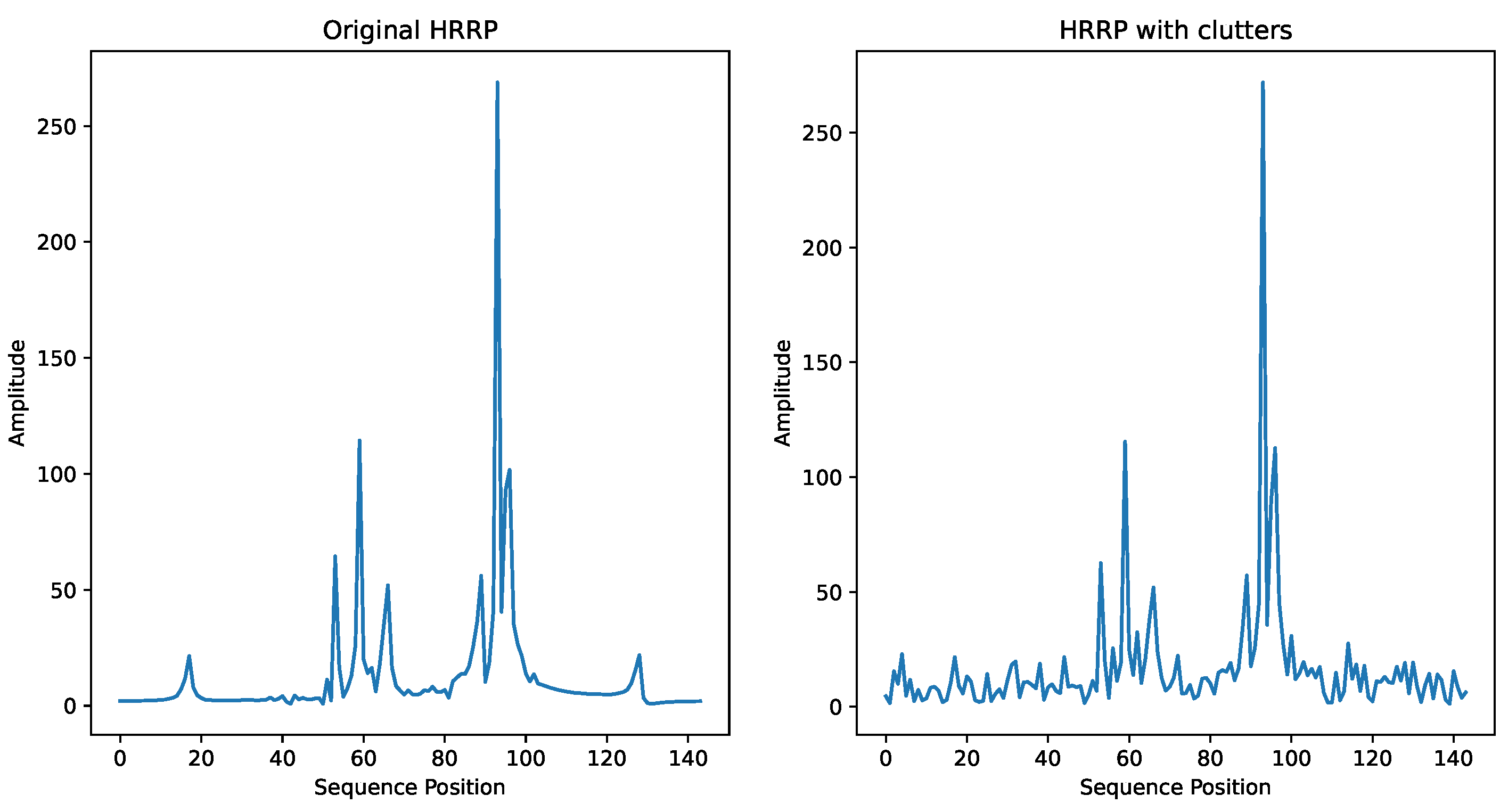
Considering the presence of ground clutter in practical scenarios, we simulate several typical ground clutter distributions, including Rayleigh distribution, log-normal distribution, Weibull distribution and K-distribution [52]. These clutter distributions are added to the HRRP echoes with a signal-to-clutter ratio of 10 dB to test the effectiveness of attention loss. Figure 11 shows an example of an HRRP sample in K-distributed clutter. The results are shown in Table 8. It can be seen that in clutter environments simulated with various distributions, using attention loss still achieves better recognition performance compared to not using it, with improvements ranging from 0.27% to 0.78%.
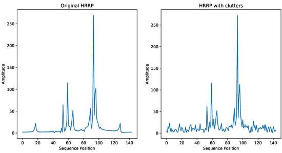
Figure 11.
A sample of HRRP with clutter.
Table 8.
Comparison of final accuracy with and without attention loss under different clutter distributions in SOC.
4.3.5. The Interpretability of Attention Loss
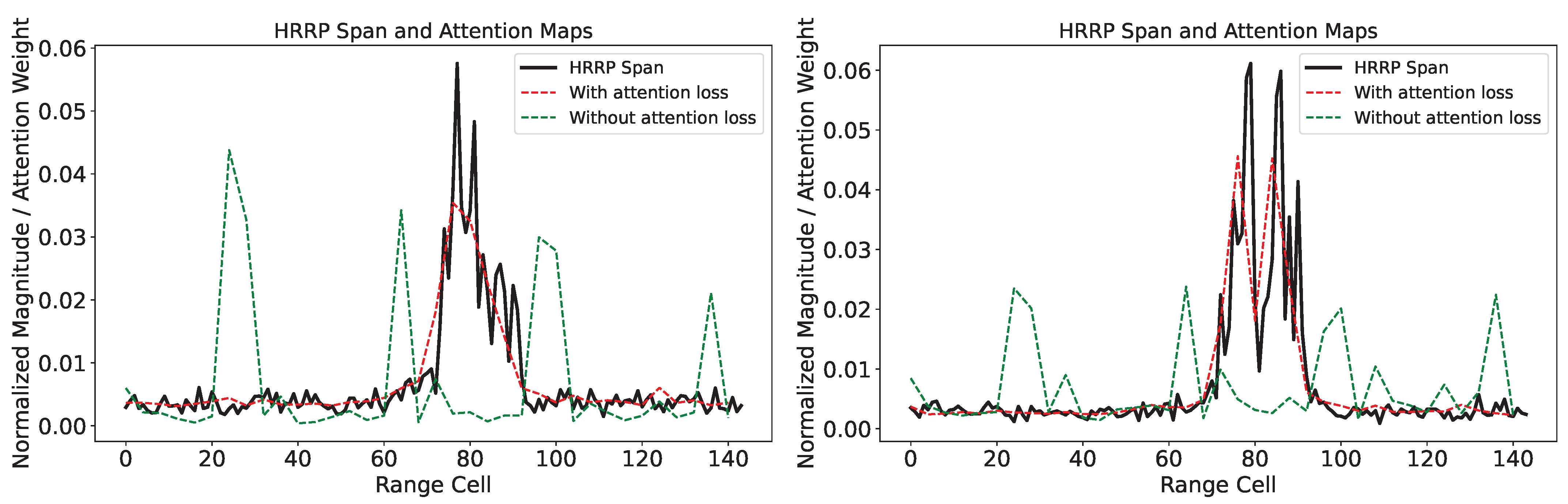
We also demonstrate the effect of attention loss through the visualization of attention maps, as shown in Figure 12. This figure presents the HRRP span along with attention maps, both with and without the application of attention loss for two samples in the test set under SOC. In the figure, the red dashed line and the black solid line follow the same trend, indicating that when using attention loss, the self-attention mechanism more effectively focuses on the strong scattering points in the HRRP. In contrast, without attention loss (represented by the green dashed line), the areas of focus are not consistently within the target regions. We need to point out that although there are notable differences in the attention maps with and without attention loss, the improvement in recognition accuracy with attention loss under SOC is not significant (as shown in Figure 9 and Table 6). In SOC, the ViT’s fitting capability, combined with the polarimetric features we extracted, is sufficient to achieve good accuracy. However, this fitting capability is not interpretable, as evidenced by the attention maps without attention loss, where the peak focuses on the background region. While the use of attention loss under SOC does not significantly improve accuracy, it does provide better interpretability, as seen in the attention maps with attention loss completely focusing on the part of the strong scattering point, which is crucial in deep learning networks. Considering that the additional computational burden introduced by attention loss is minimal, it is still beneficial to use attention loss in SOC. In contrast, under EOC, where the observation conditions between the training and testing sets vary greatly, the fitting capability of ViT alone is insufficient to maintain accuracy. The use of attention loss helps the network focus more on the target region, resulting in a more noticeable effect of attention loss under EOC (as shown in Figure 10 and Table 7) compared to SOC. This highlights the effectiveness of our method in more complex environments and experimental conditions.
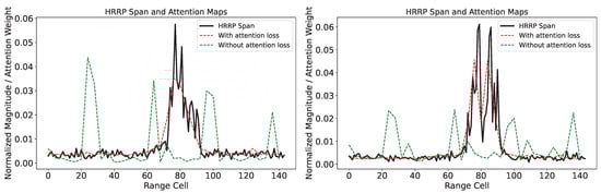
Figure 12.
Visualization of the effect of attention loss.
5. Conclusions
In this study, we propose an ITAViT model: a novel approach for polarimetric HRRP target recognition, leveraging the ViT enhanced by polarimetric preprocessing and a specifically designed attention loss. We implement various manual polarimetric feature extractions and also derive the back-propagation process for attention loss. Through extensive testing on a dataset of simulated X-band signatures of civilian vehicles, our method demonstrates overall superior performance compared to other approaches used for HRRP target recognition, achieving the highest recognition rates when considering both SOC and EOC conditions. We also conduct ablation experiments to test the effects of polarimetric preprocessing and attention loss separately. The results indicate that the combination of magnitude and coherent features achieves better recognition rates compared to other methods utilizing polarimetric information, and the PPL further enhances performance by extracting additional polarimetric features. The use of attention loss improves recognition rates under SOC, EOC, and simulated ground clutter environments by guiding the network to focus on the strong scattering points of the target, enhancing the model’s generalization performance, robustness to noisy environments, and interpretability.
Although our approach marks a significant achievement, we recognize its limitations. First, in some radar data, the weak scattering points of a target may also carry important information, such as the target’s shape and size. Our method with attention loss might lose some of this information. To address this limitation, we plan to explore additional mechanisms in future work that can balance the attention given to both strong and weak radar signals. For instance, we consider developing a weighted attention loss or an adaptive approach that better captures the full spectrum of radar data. Besides, given the absence of actual polarimetric HRRP datasets, our experiments are limited to simulated data with added noise and clutter for testing. Future work will involve acquiring real polarimetric HRRP datasets to evaluate the network’s performance in practical scenarios. Finally, the attention loss shows promising results for HRRP data but may not be directly transferred into image domain applications due to its tailored design for HRRP. Future work will focus on exploring the potential of attention loss.
Author Contributions
Conceptualization, F.G. and J.Y.; methodology, F.G.; software, F.G. and P.L.; validation, P.L. and Z.L.; formal analysis, F.G. and P.L.; investigation, F.G. and Z.L.; resources, C.Y. and J.Y.; data curation, C.Y. and F.G.; writing—original draft preparation, F.G. and P.L.; writing—review and editing, P.L. and D.R.; visualization, D.R.; supervision, P.L. and Z.L.; project administration, J.Y.; funding acquisition, C.Y. and J.Y. All authors have read and agreed to the published version of the manuscript.
Funding
This work was partly supported by NSFC under Grant no. 62222102 and NSFC Grant no. 62171023.
Data Availability Statement
The original data presented in the study are openly available in https://www.sdms.afrl.af.mil/index.php?collection=cv_dome, accessed on 6 January 2024.
Conflicts of Interest
The authors declare no conflicts of interest.
Abbreviations
The following abbreviations are used in this manuscript:
| ConvLSTM | Convolutional Long Short-Term Memory |
| CNN | Convolutional Neural Network |
| EOC | Extended Operating Condition |
| HRRP | High-Resolution Range Profile |
| ISAR | Inverse Synthetic Aperture Radar |
| ITAViT | Interpretable Target-Aware Vision Transformer |
| LSTM | Long Short-Term Memory network |
| MSE | Mean Square Error |
| PPL | Polarimetric Preprocessing Layer |
| PwAET | Patch-wise Auto-Encoder based on Transformers |
| RATR | Radar Automatic Target Recognition |
| RNN | Recurrent Neural Network |
| SAR | Synthetic Aperture Radar |
| SCRAM | Stacked CNN–Bi-RNN with an Attention Mechanism |
| SNR | Signal-to-Noise Ratio |
| SOC | Standard Operating Condition |
| TACNN | Target-Attentional Convolutional Neural Network |
| TARAN | Target-Aware Recurrent Attentional Network |
| t-SNE | t-distributed Stochastic Neighbor Rmbedding |
| ViT | Vision Transformer |
References
- Huang, Z.; Pan, Z.; Lei, B. What, Where, and How to Transfer in SAR Target Recognition Based on Deep CNNs. IEEE Trans. Geosci. Remote Sens. 2020, 58, 2324–2336. [Google Scholar] [CrossRef]
- Zhang, J.; Xing, M.; Xie, Y. FEC: A Feature Fusion Framework for SAR Target Recognition Based on Electromagnetic Scattering Features and Deep CNN Features. IEEE Trans. Geosci. Remote Sens. 2021, 59, 2174–2187. [Google Scholar] [CrossRef]
- Jiang, W.; Wang, Y.; Li, Y.; Lin, Y.; Shen, W. Radar target characterization and deep learning in radar automatic target recognition: A review. Remote Sens. 2023, 15, 3742. [Google Scholar] [CrossRef]
- Cao, X.; Yi, J.; Gong, Z.; Wan, X. Automatic Target Recognition Based on RCS and Angular Diversity for Multistatic Passive Radar. IEEE Trans. Aerosp. Electron. Syst. 2022, 58, 4226–4240. [Google Scholar] [CrossRef]
- Abadpour, S.; Pauli, M.; Schyr, C.; Klein, F.; Degen, R.; Siska, J.; Pohl, N.; Zwick, T. Angular Resolved RCS and Doppler Analysis of Human Body Parts in Motion. IEEE Trans. Microw. Theory Tech. 2023, 71, 1761–1771. [Google Scholar] [CrossRef]
- Ezuma, M.; Anjinappa, C.K.; Semkin, V.; Guvenc, I. Comparative Analysis of Radar-Cross-Section- Based UAV Recognition Techniques. IEEE Sens. J. 2022, 22, 17932–17949. [Google Scholar] [CrossRef]
- Wang, Z.; Yu, Z.; Lou, X.; Guo, B.; Chen, L. Gesture-Radar: A Dual Doppler Radar Based System for Robust Recognition and Quantitative Profiling of Human Gestures. IEEE Trans. Hum.-Mach. Syst. 2021, 51, 32–43. [Google Scholar] [CrossRef]
- Xu, X.; Feng, C.; Han, L. Classification of Radar Targets with Micro-Motion Based on RCS Sequences Encoding and Convolutional Neural Network. Remote Sens. 2022, 14, 5863. [Google Scholar] [CrossRef]
- Qiao, X.; Li, G.; Shan, T.; Tao, R. Human Activity Classification Based on Moving Orientation Determining Using Multistatic Micro-Doppler Radar Signals. IEEE Trans. Geosci. Remote Sens. 2022, 60, 5104415. [Google Scholar] [CrossRef]
- Wang, H.; Xing, C.; Yin, J.; Yang, J. Land cover classification for polarimetric SAR images based on vision transformer. Remote Sens. 2022, 14, 4656. [Google Scholar] [CrossRef]
- Li, J.; Yu, Z.; Yu, L.; Cheng, P.; Chen, J.; Chi, C. A comprehensive survey on SAR ATR in deep-learning era. Remote Sens. 2023, 15, 1454. [Google Scholar] [CrossRef]
- Zheng, J.; Li, M.; Li, X.; Zhang, P.; Wu, Y. Revisiting Local and Global Descriptor-Based Metric Network for Few-Shot SAR Target Classification. IEEE Trans. Geosci. Remote Sens. 2024, 62, 5205814. [Google Scholar] [CrossRef]
- Cai, J.; Martorella, M.; Liu, Q.; Ding, Z.; Giusti, E.; Long, T. Automatic target recognition based on alignments of three-dimensional interferometric ISAR images and CAD models. IEEE Trans. Aerosp. Electron. Syst. 2020, 56, 4872–4888. [Google Scholar] [CrossRef]
- Zhang, Y.; Yuan, H.; Li, H.; Chen, J.; Niu, M. Meta-Learner-Based Stacking Network on Space Target Recognition for ISAR Images. IEEE J. Sel. Top. Appl. Earth Obs. Remote Sens. 2021, 14, 12132–12148. [Google Scholar] [CrossRef]
- Yuan, H.; Li, H.; Zhang, Y.; Wei, C.; Gao, R. Complex-Valued Multiscale Vision Transformer on Space Target Recognition by ISAR Image Sequence. IEEE Geosci. Remote Sens. Lett. 2024, 21, 4008305. [Google Scholar] [CrossRef]
- Shi, L.; Wang, P.; Liu, H.; Xu, L.; Bao, Z. Radar HRRP Statistical Recognition With Local Factor Analysis by Automatic Bayesian Ying-Yang Harmony Learning. IEEE Trans. Signal Process. 2011, 59, 610–617. [Google Scholar] [CrossRef]
- Du, L.; Chen, J.; Hu, J.; Li, Y.; He, H. Statistical Modeling With Label Constraint for Radar Target Recognition. IEEE Trans. Aerosp. Electron. Syst. 2020, 56, 1026–1044. [Google Scholar] [CrossRef]
- Persico, A.R.; Ilioudis, C.V.; Clemente, C.; Soraghan, J.J. Novel Classification Algorithm for Ballistic Target Based on HRRP Frame. IEEE Trans. Aerosp. Electron. Syst. 2019, 55, 3168–3189. [Google Scholar] [CrossRef]
- Chen, J.; Du, L.; He, H.; Guo, Y. Convolutional factor analysis model with application to radar automatic target recognition. Pattern Recognit. 2019, 87, 140–156. [Google Scholar] [CrossRef]
- Guo, D.; Chen, B.; Chen, W.; Wang, C.; Liu, H.; Zhou, M. Variational Temporal Deep Generative Model for Radar HRRP Target Recognition. IEEE Trans. Signal Process. 2020, 68, 5795–5809. [Google Scholar] [CrossRef]
- Chen, W.; Chen, B.; Peng, X.; Liu, J.; Yang, Y.; Zhang, H.; Liu, H. Tensor RNN with Bayesian Nonparametric Mixture for Radar HRRP Modeling and Target Recognition. IEEE Trans. Signal Process. 2021, 69, 1995–2009. [Google Scholar] [CrossRef]
- Li, H.J.; Yang, S.H. Using range profiles as feature vectors to identify aerospace objects. IEEE Trans. Antennas Propag. 1993, 41, 261–268. [Google Scholar] [CrossRef]
- Du, L.; Liu, H.; Bao, Z. Radar HRRP Statistical Recognition: Parametric Model and Model Selection. IEEE Trans. Signal Process. 2008, 56, 1931–1944. [Google Scholar] [CrossRef]
- Du, L.; Liu, H.; Wang, P.; Feng, B.; Pan, M.; Bao, Z. Noise Robust Radar HRRP Target Recognition Based on Multitask Factor Analysis with Small Training Data Size. IEEE Trans. Signal Process. 2012, 60, 3546–3559. [Google Scholar] [CrossRef]
- Du, L.; Liu, H.; Bao, Z.; Xing, M. Radar HRRP target recognition based on higher order spectra. IEEE Trans. Signal Process. 2005, 53, 2359–2368. [Google Scholar] [CrossRef]
- Pan, M.; Du, L.; Wang, P.; Liu, H.; Bao, Z. Multi-task hidden Markov model for radar automatic target recognition. In Proceedings of the 2011 IEEE CIE International Conference on Radar, Chengdu, China, 24–27 October 2011; Volume 1, pp. 650–653. [Google Scholar] [CrossRef]
- Mian, P.; Jie, J.; Zhu, L.; Jing, C.; Tao, Z. Radar HRRP recognition based on discriminant deep autoencoders with small training data size. Electron. Lett. 2016, 52, 1725–1727. [Google Scholar] [CrossRef]
- Du, C.; Chen, B.; Xu, B.; Guo, D.; Liu, H. Factorized discriminative conditional variational auto-encoder for radar HRRP target recognition. Signal Process. 2019, 158, 176–189. [Google Scholar] [CrossRef]
- Zhang, X.; Wei, Y.; Wang, W. Patch-Wise Autoencoder Based on Transformer for Radar High-Resolution Range Profile Target Recognition. IEEE Sens. J. 2023, 23, 29406–29414. [Google Scholar] [CrossRef]
- Wan, J.; Chen, B.; Xu, B.; Liu, H.; Jin, L. Convolutional neural networks for radar HRRP target recognition and rejection. Eurasip J. Adv. Signal Process. 2019, 2019, 5. [Google Scholar] [CrossRef]
- Fu, Z.; Li, S.; Li, X.; Dan, B.; Wang, X. A neural network with convolutional module and residual structure for radar target recognition based on high-resolution range profile. Sensors 2020, 20, 586. [Google Scholar] [CrossRef] [PubMed]
- Chen, J.; Du, L.; Guo, G.; Yin, L.; Wei, D. Target-attentional CNN for radar automatic target recognition with HRRP. Signal Process. 2022, 196, 108497. [Google Scholar] [CrossRef]
- Xu, B.; Chen, B.; Wan, J.; Liu, H.; Jin, L. Target-aware recurrent attentional network for radar HRRP target recognition. Signal Process. 2019, 155, 268–280. [Google Scholar] [CrossRef]
- Zhang, L.; Li, Y.; Wang, Y.; Wang, J.; Long, T. Polarimetric HRRP recognition based on ConvLSTM with self-attention. IEEE Sens. J. 2020, 21, 7884–7898. [Google Scholar] [CrossRef]
- Pan, M.; Liu, A.; Yu, Y.; Wang, P.; Li, J.; Liu, Y.; Lv, S.; Zhu, H. Radar HRRP target recognition model based on a stacked CNN–Bi-RNN with attention mechanism. IEEE Trans. Geosci. Remote Sens. 2021, 60, 5100814. [Google Scholar] [CrossRef]
- Diao, Y.; Liu, S.; Gao, X.; Liu, A. Position Embedding-Free Transformer for Radar HRRP Target Recognition. In Proceedings of the IGARSS 2022–2022 IEEE International Geoscience and Remote Sensing Symposium, Kuala Lumpur, Malaysia, 17–22 July 2022; pp. 1896–1899. [Google Scholar]
- Long, T.; Zhang, L.; Li, Y.; Wang, Y. Geometrical Structure Classification of Target HRRP Scattering Centers Based on Dual Polarimetric H/α Features. IEEE Access 2019, 7, 141679–141688. [Google Scholar] [CrossRef]
- Yang, W.; Zhou, Q.; Yuan, M.; Li, Y.; Wang, Y.; Zhang, L. Dual-band polarimetric HRRP recognition via a brain-inspired multi-channel fusion feature extraction network. Front. Neurosci. 2023, 17, 1252179. [Google Scholar] [CrossRef]
- Zhang, L.; Han, C.; Wang, Y.; Li, Y.; Long, T. Polarimetric HRRP recognition based on feature-guided Transformer model. Electron. Lett. 2021, 57, 705–707. [Google Scholar] [CrossRef]
- Yang, X.; Wen, G.; Ma, C.; Hui, B.; Ding, B.; Zhang, Y. CFAR Detection of Moving Range-Spread Target in White Gaussian Noise Using Waveform Contrast. IEEE Geosci. Remote Sens. Lett. 2016, 13, 282–286. [Google Scholar] [CrossRef]
- Dosovitskiy, A.; Beyer, L.; Kolesnikov, A.; Weissenborn, D.; Zhai, X.; Unterthiner, T.; Dehghani, M.; Minderer, M.; Heigold, G.; Gelly, S. An Image is Worth 16x16 Words: Transformers for Image Recognition at Scale. In Proceedings of the International Conference on Learning Representations, Vienna, Austria, 4 May 2021. [Google Scholar]
- Vaswani, A.; Shazeer, N.; Parmar, N.; Uszkoreit, J.; Jones, L.; Gomez, A.N.; Kaiser, Ł.; Polosukhin, I. Attention is all you need. arXiv 2017, arXiv:1706.03762. [Google Scholar] [CrossRef]
- Xiao, T.; Singh, M.; Mintun, E.; Darrell, T.; Dollár, P.; Girshick, R. Early convolutions help transformers see better. Proc. Adv. Neural Inf. Process. Syst. 2021, 34, 30392–30400. [Google Scholar]
- Gao, F.; Ren, D.; Yin, J.; Yang, J. Polarimetric HRRP recognition using vision Transformer with polarimetric preprocessing and attention loss. In Proceedings of the IEEE International Geoscience and Remote Sensing Symposium proceedings (IGARSS), Athens, Greece, 7–12 July 2024. [Google Scholar]
- Cumming, I.G.; Wong, F.H. Digital processing of synthetic aperture radar data. Artech House 2005, 1, 108–110. [Google Scholar]
- Akyildiz, Y.; Moses, R.L. Scattering center model for SAR imagery. In Proceedings of the SAR Image Analysis, Modeling, and Techniques II, Florence, Italy, 20–24 September 1999; Volume 3869, pp. 76–85. [Google Scholar]
- Lang, P.; Fu, X.; Dong, J.; Yang, J. An efficient radon Fourier transform-based coherent integration method for target detection. IEEE Geosci. Remote Sens. Lett. 2023, 20, 3501905. [Google Scholar] [CrossRef]
- Lee, J.S.; Pottier, E. Polarimetric Radar Imaging: From Basics to Applications; CRC Press: Boca Raton, FL, USA, 2017. [Google Scholar]
- He, L. The Full Derivation of Transformer Gradient. GitHub Repository. 2022. Available online: https://github.com/Say-Hello2y/Transformer-attention (accessed on 10 June 2024).
- Potter, L.; Nehrbass, J.; Dungan, K. CVDomes: A Data Set of Simulated X-Band Signatures of Civilian Vehicles; Air Force Research Laboratory: Greene County, OH, USA, 2009. [Google Scholar]
- Van der Maaten, L.; Hinton, G. Visualizing data using t-SNE. J. Mach. Learn. Res. 2008, 9, 2579–2605. [Google Scholar]
- Billingsley, J.; Farina, A.; Gini, F.; Greco, M.; Verrazzani, L. Statistical analyses of measured radar ground clutter data. IEEE Trans. Aerosp. Electron. Syst. 1999, 35, 579–593. [Google Scholar] [CrossRef]


Disclaimer/Publisher’s Note: The statements, opinions and data contained in all publications are solely those of the individual author(s) and contributor(s) and not of MDPI and/or the editor(s). MDPI and/or the editor(s) disclaim responsibility for any injury to people or property resulting from any ideas, methods, instructions or products referred to in the content. |
© 2024 by the authors. Licensee MDPI, Basel, Switzerland. This article is an open access article distributed under the terms and conditions of the Creative Commons Attribution (CC BY) license (https://creativecommons.org/licenses/by/4.0/).