
Accurate Deformation Retrieval of the 2023 Turkey–Syria Earthquakes Using Multi-Track InSAR Data and a Spatio-Temporal Correlation Analysis with the ICA Method


Abstract
1. Introduction
2. Methods
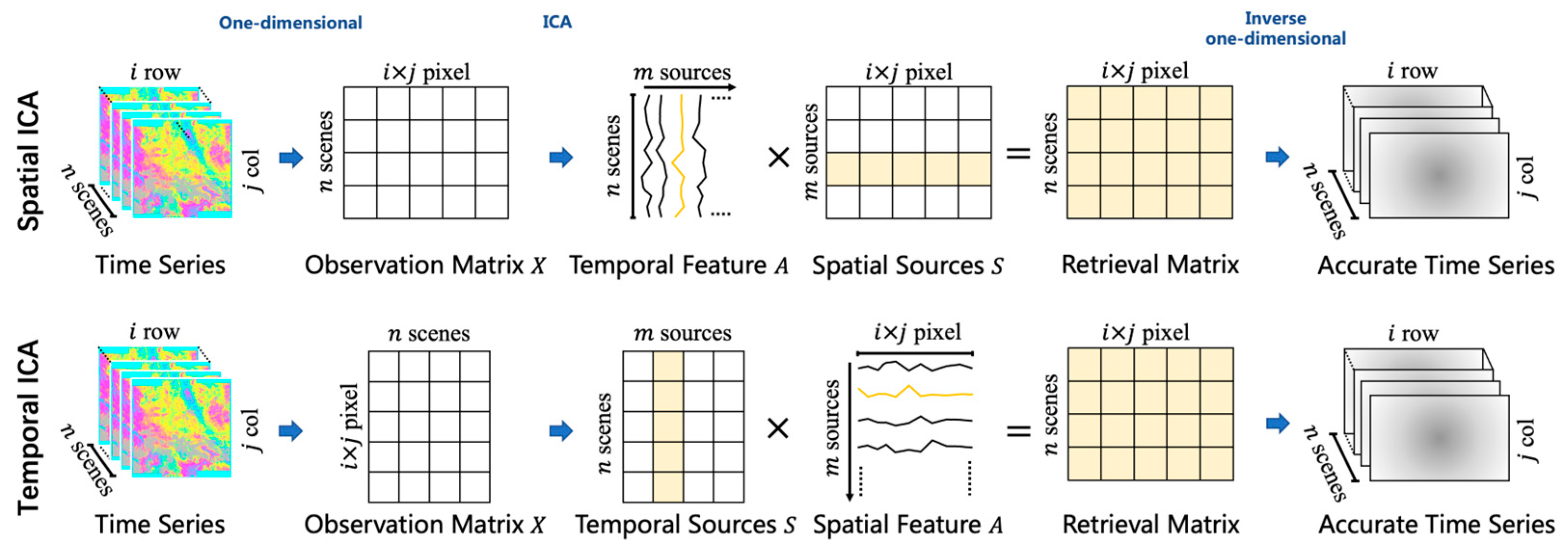
2.1. Independent Component Analysis
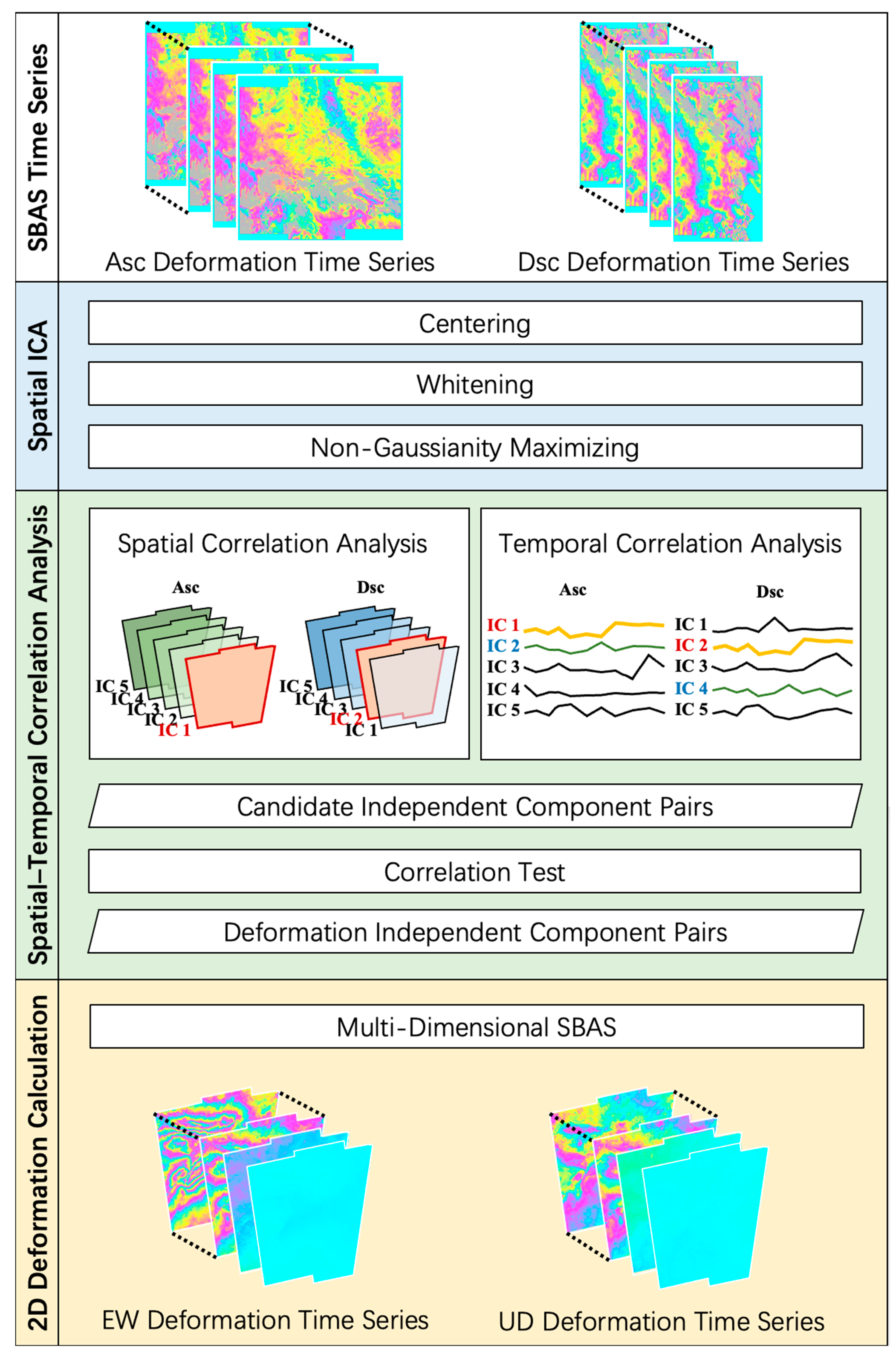
2.2. Spatio-Temporal Correlation Analysis
2.3. Multi-Dimensional Small Baseline Subset
3. Study Area and Dataset
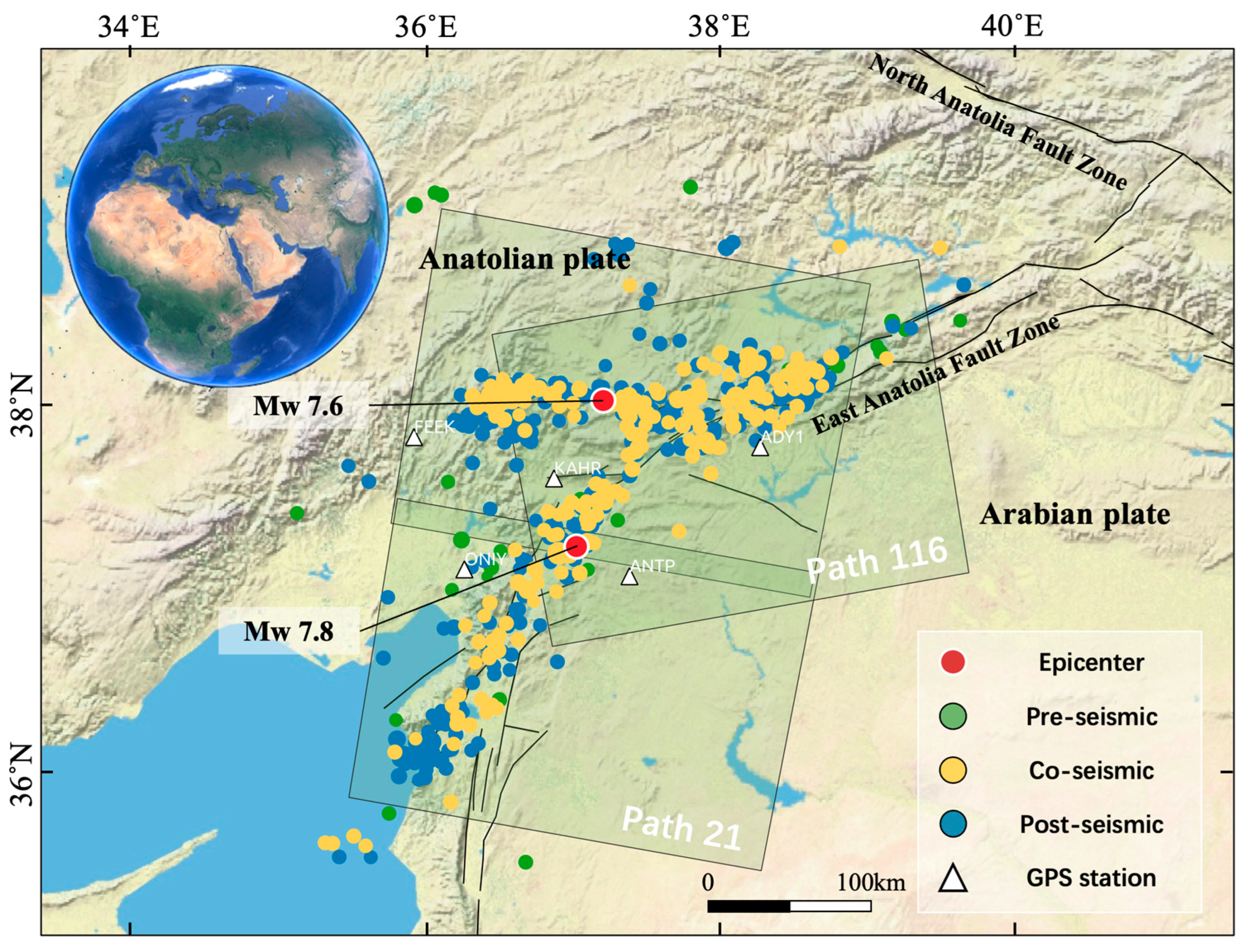
3.1. Study Area
3.2. Dataset
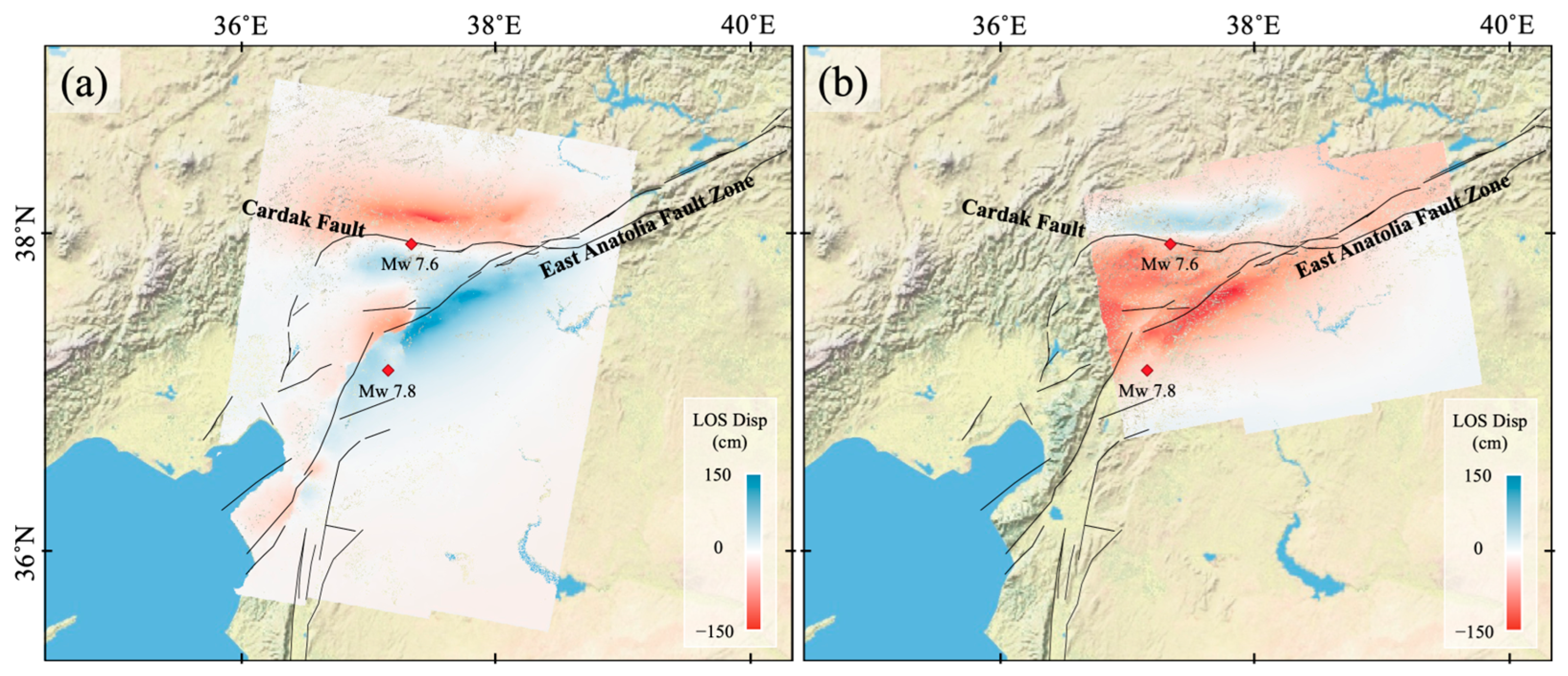
4. Results and Discussion
5. Conclusions
Author Contributions
Funding
Data Availability Statement
Acknowledgments
Conflicts of Interest
References
- Rosen, P.A.; Hensley, S.; Joughin, I.R.; Li, F.K.; Madsen, S.N.; Rodriguez, E.; Goldstein, R.M. Synthetic Aperture Radar Interferometry. Proc. IEEE 2000, 88, 333–382. [Google Scholar] [CrossRef]
- Wang, C.; Chang, L.; Wang, X.-S.; Zhang, B.; Stein, A. Interferometric Synthetic Aperture Radar Statistical Inference in Deformation Measurement and Geophysical Inversion: A Review. In IEEE Geoscience and Remote Sensing Magazine; IEEE: Piscataway, NJ, USA, 2024. [Google Scholar]
- Wang, C.; Wei, M.; Qin, X.; Li, T.; Chen, S.; Zhu, C.; Liu, P.; Chang, L. Three-Dimensional Lookup Table for More Precise SAR Scatterers Positioning in Urban Scenarios. ISPRS J. Photogramm. Remote Sens. 2024, 209, 133–149. [Google Scholar] [CrossRef]
- Massonnet, D.; Rossi, M.; Carmona, C.; Adragna, F.; Peltzer, G.; Feigl, K.; Rabaute, T. The Displacement Field of the Landers Earthquake Mapped by Radar Interferometry. Nature 1993, 364, 138–142. [Google Scholar] [CrossRef]
- Zhang, B.; Ding, X.; Amelung, F.; Wang, C.; Xu, W.; Zhu, W.; Shimada, M.; Zhang, Q.; Baba, T. Impact of Ionosphere on InSAR Observation and Coseismic Slip Inversion: Improved Slip Model for the 2010 Maule, Chile, Earthquake. Remote Sens. Environ. 2021, 267, 112733. [Google Scholar] [CrossRef]
- Agram, P.; Simons, M. A Noise Model for InSAR Time Series. J. Geophys. Res. Solid Earth 2015, 120, 2752–2771. [Google Scholar] [CrossRef]
- Zebker, H.A.; Rosen, P.A.; Hensley, S. Atmospheric Effects in Interferometric Synthetic Aperture Radar Surface Deformation and Topographic Maps. J. Geophys. Res. Solid Earth 1997, 102, 7547–7563. [Google Scholar] [CrossRef]
- Fuhrmann, T.; Garthwaite, M.C. Resolving Three-Dimensional Surface Motion with InSAR: Constraints from Multi-Geometry Data Fusion. Remote Sens. 2019, 11, 241. [Google Scholar] [CrossRef]
- Li, Z.; Muller, J.-P.; Cross, P. Tropospheric Correction Techniques in Repeat-Pass SAR Interferometry; ESA ESRIN: Frascati, Italy, 2003; pp. 1–5. [Google Scholar]
- Hopfield, H.S. Tropospheric Effect on Electromagnetically Measured Range: Prediction from Surface Weather Data. Radio Sci. 1971, 6, 357–367. [Google Scholar] [CrossRef]
- Bock, Y.; Williams, S. Integrated Satellite Interferometry in Southern California. Eos Trans. Am. Geophys. Union 1997, 78, 293–300. [Google Scholar] [CrossRef]
- Chaabane, F.; Avallone, A.; Tupin, F.; Briole, P.; Maître, H. A Multitemporal Method for Correction of Tropospheric Effects in Differential SAR Interferometry: Application to the Gulf of Corinth Earthquake. IEEE Trans. Geosci. Remote Sens. 2007, 45, 1605–1615. [Google Scholar] [CrossRef]
- Ding, X.; Li, Z.; Zhu, J.; Feng, G.; Long, J. Atmospheric Effects on InSAR Measurements and Their Mitigation. Sensors 2008, 8, 5426–5448. [Google Scholar] [CrossRef]
- Fielding, E.J.; Lundgren, P.R.; Taymaz, T.; Yolsal-Çevikbilen, S.; Owen, S.E. Fault-slip Source Models for the 2011 M 7.1 Van Earthquake in Turkey from SAR Interferometry, Pixel Offset Tracking, GPS, and Seismic Waveform Analysis. Seismol. Res. Lett. 2013, 84, 579–593. [Google Scholar] [CrossRef]
- Wang, X.; Liu, G.; Yu, B.; Dai, K.; Zhang, R.; Chen, Q.; Li, Z. 3D Coseismic Deformations and Source Parameters of the 2010 Yushu Earthquake (China) Inferred from DInSAR and Multiple-Aperture InSAR Measurements. Remote Sens. Environ. 2014, 152, 174–189. [Google Scholar] [CrossRef]
- Samsonov, S.V.; d’Oreye, N. Multidimensional Small Baseline Subset (MSBAS) for Two-Dimensional Deformation Analysis: Case Study Mexico City. Can. J. Remote Sens. 2017, 43, 318–329. [Google Scholar] [CrossRef]
- Yang, C.; Han, B.; Zhao, C.; Du, J.; Zhang, D.; Zhu, S. Co-and Post-Seismic Deformation Mechanisms of the MW 7.3 Iran Earthquake (2017) Revealed by Sentinel-1 InSAR Observations. Remote Sens. 2019, 11, 418. [Google Scholar] [CrossRef]
- Kirui, P.K.; Reinosch, E.; Isya, N.; Riedel, B.; Gerke, M. Mitigation of Atmospheric Artefacts in Multi Temporal InSAR: A Review. Remote Sens. Geoinf. Sci. 2021, 89, 251–272. [Google Scholar] [CrossRef]
- Xiao, R.; Yu, C.; Li, Z.; He, X. Statistical Assessment Metrics for InSAR Atmospheric Correction: Applications to Generic Atmospheric Correction Online Service for InSAR (GACOS) in Eastern China. Int. J. Appl. Earth Obs. Geoinf. 2021, 96, 102289. [Google Scholar] [CrossRef]
- Jolivet, R.; Agram, P.S.; Lin, N.Y.; Simons, M.; Doin, M.; Peltzer, G.; Li, Z. Improving InSAR Geodesy Using Global Atmospheric Models. J. Geophys. Res. Solid Earth 2014, 119, 2324–2341. [Google Scholar] [CrossRef]
- Li, Z.; Duan, M.; Cao, Y.; Mu, M.; He, X.; Wei, J. Mitigation of Time-Series InSAR Turbulent Atmospheric Phase Noise: A Review. Geod. Geodyn. 2022, 13, 93–103. [Google Scholar] [CrossRef]
- Ebmeier, S.K. Application of Independent Component Analysis to Multitemporal InSAR Data with Volcanic Case Studies: ICA Analysis of InSAR Data. J. Geophys. Res. Solid Earth 2016, 121, 8970–8986. [Google Scholar] [CrossRef]
- Maubant, L.; Pathier, E.; Daout, S.; Radiguet, M.; Doin, M.-P.; Kazachkina, E.; Kostoglodov, V.; Cotte, N.; Walpersdorf, A. Independent Component Analysis and Parametric Approach for Source Separation in InSAR Time Series at Regional Scale: Application to the 2017–2018 Slow Slip Event in Guerrero (Mexico). J. Geophys. Res. Solid Earth 2020, 125, e2019JB018187. [Google Scholar] [CrossRef]
- Peng, M.; Motagh, M.; Lu, Z.; Xia, Z.; Guo, Z.; Zhao, C.; Liu, Q. Characterization and Prediction of InSAR-Derived Ground Motion with ICA-Assisted LSTM Model. Remote Sens. Environ. 2024, 301, 113923. [Google Scholar] [CrossRef]
- Cohen-Waeber, J.; Bürgmann, R.; Chaussard, E.; Giannico, C.; Ferretti, A. Spatiotemporal Patterns of Precipitation-modulated Landslide Deformation from Independent Component Analysis of InSAR Time Series. Geophys. Res. Lett. 2018, 45, 1878–1887. [Google Scholar] [CrossRef]
- Hyvärinen, A.; Oja, E. Independent Component Analysis: Algorithms and Applications. Neural Netw. 2000, 13, 411–430. [Google Scholar] [CrossRef]
- Comon, P. Independent Component Analysis, A New Concept? Signal Process. 1994, 36, 287–314. [Google Scholar] [CrossRef]
- Kumar, M.; Jayanthi, V. Blind Source Separation Using Kurtosis, Negentropy and Maximum Likelihood Functions. Int. J. Speech Technol. 2020, 23, 13–21. [Google Scholar] [CrossRef]
- Liang, H.; Zhang, L.; Lu, Z.; Li, X. Nonparametric Estimation of DEM Error in Multitemporal InSAR. IEEE Trans. Geosci. Remote Sens. 2019, 57, 10004–10014. [Google Scholar] [CrossRef]
- Kanji, G.K. 100 Statistical Tests; SAGE Publications Ltd.: Thousand Oaks, CA, USA, 2006; pp. 1–256. [Google Scholar]
- Samsonov, S.; d’Oreye, N. Multidimensional Time-Series Analysis of Ground Deformation from Multiple InSAR Data Sets Applied to Virunga Volcanic Province. Geophys. J. Int. 2012, 191, 1095–1108. [Google Scholar]
- He, L.; Feng, G.; Xu, W.; Wang, Y.; Xiong, Z.; Gao, H.; Liu, X. Coseismic Kinematics of the 2023 Kahramanmaras, Turkey Earthquake Sequence from InSAR and Optical Data. Geophys. Res. Lett. 2023, 50, e2023GL104693. [Google Scholar] [CrossRef]
- Zhao, J.-J.; Chen, Q.; Yang, Y.-H.; Xu, Q. Coseismic Faulting Model and Post-Seismic Surface Motion of the 2023 Turkey–Syria Earthquake Doublet Revealed by InSAR and GPS Measurements. Remote Sens. 2023, 15, 3327. [Google Scholar] [CrossRef]
- Emre, Ö.; Kondo, H.; Özalp, S.; Elmacı, H. Fault Geometry, Segmentation and Slip Distribution Associated with the 1939 Erzincan Earthquake Rupture along the North Anatolian Fault, Turkey; Geological Society: London, UK, 2021. [Google Scholar]
- Reilinger, R.; McClusky, S.; Vernant, P.; Lawrence, S.; Ergintav, S.; Cakmak, R.; Ozener, H.; Kadirov, F.; Guliev, I.; Stepanyan, R. GPS Constraints on Continental Deformation in the Africa-Arabia-Eurasia Continental Collision Zone and Implications for the Dynamics of Plate Interactions. J. Geophys. Res. Solid Earth 2006, 111. [Google Scholar] [CrossRef]
- Marza, V.I. On the Death Toll of the 1999 Izmit (Turkey) Major Earthquake; ESC General Assembly Papers; European Seismological Commission: Potsdam, Germany, 2004. [Google Scholar]
- Hubert-Ferrari, A.; Lamair, L.; Hage, S.; Schmidt, S.; Çağatay, M.N.; Avşar, U. A 3800 Yr Paleoseismic Record (Lake Hazar Sediments, Eastern Turkey): Implications for the East Anatolian Fault Seismic Cycle. Earth Planet. Sci. Lett. 2020, 538, 116152. [Google Scholar] [CrossRef]
- Chen, J.; Zhou, Y. Coseismic Slip Distribution of the 2023 Earthquake Doublet in Turkey and Syria from Joint Inversion of Sentinel-1 and Sentinel-2 Data: An Iterative Modeling Method for Mapping Large Earthquake Deformation. Geophys. J. Int. 2024, 237, 636–648. [Google Scholar] [CrossRef]
- Dai, X.; Liu, X.; Liu, R.; Song, M.; Zhu, G.; Chang, X.; Guo, J. Coseismic Slip Distribution and Coulomb Stress Change of the 2023 MW 7.8 Pazarcik and MW 7.5 Elbistan Earthquakes in Turkey. Remote Sens. 2024, 16, 240. [Google Scholar] [CrossRef]
- Jia, Z.; Jin, Z.; Marchandon, M.; Ulrich, T.; Gabriel, A.-A.; Fan, W.; Shearer, P.; Zou, X.; Rekoske, J.; Bulut, F. The Complex Dynamics of the 2023 Kahramanmaraş, Turkey, M w 7.8-7.7 Earthquake Doublet. Science 2023, 381, 985–990. [Google Scholar] [CrossRef]
- Li, S.; Wang, X.; Tao, T.; Zhu, Y.; Qu, X.; Li, Z.; Huang, J.; Song, S. Source Model of the 2023 Turkey Earthquake Sequence Imaged by Sentinel-1 and GPS Measurements: Implications for Heterogeneous Fault Behavior along the East Anatolian Fault Zone. Remote Sens. 2023, 15, 2618. [Google Scholar] [CrossRef]
- Bondur, V.; Chimitdorzhiev, T.; Dmitriev, A. Assessment of Anomalous Geodynamics before the 2023 Mw 7.8 Earthquake in Turkey by Stacking-InSAR Method. Izv. Atmos. Ocean. Phys. 2023, 59, 1001–1008. [Google Scholar] [CrossRef]
- Zhang, L.; Hu, J.; Ding, X.; Wen, Y.; Liang, H. Estimation of Coseismic Deformation with Multitemporal Radar Interferometry. IEEE Geosci. Remote Sens. Lett. 2021, 19, 1–5. [Google Scholar] [CrossRef]

| Path | Pass Direction | Frame | Date | No. of SLCs | No. of Interferograms | Incident Angle | Azimuth Angle |
|---|---|---|---|---|---|---|---|
| 116 | Ascending | 119 | 20220104–20230710 | 46 | 376 | 33.82° | −13.23° |
| 21 | Descending | 465,471 | 20220110–20230716 | 46 | 374 | 22.83° | −166.72° |
| Path | Pass Direction | Master | Slave | Perpendicular Baseline (m) | Temporal Baseline (Days) |
|---|---|---|---|---|---|
| 116 | Ascending | 20230204 | 20230229 | 113.54 | 24 |
| 21 | Descending | 20230129 | 20230210 | 111.19 | 12 |
| Path | Station | Original MSBAS STD (cm) | Proposed Method STD (cm) | Ratio |
|---|---|---|---|---|
| Asc | ADY1 | 0.0022 | 0.0020 | 7.10% |
| Asc | ANTP | Ref | Ref | Ref |
| Asc | KAHR | 0.0177 | 0.0112 | 36.86% |
| Dsc | ADY1 | 0.0137 | 0.0104 | 24.46% |
| Dsc | ANTP | Ref | Ref | Ref |
| Dsc | FEEK | 0.0127 | 0.0077 | 39.20% |
| Dsc | KAHR | 0.0274 | 0.0228 | 16.50% |
| Dsc | ONIY | 0.0175 | 0.0139 | 20.70% |
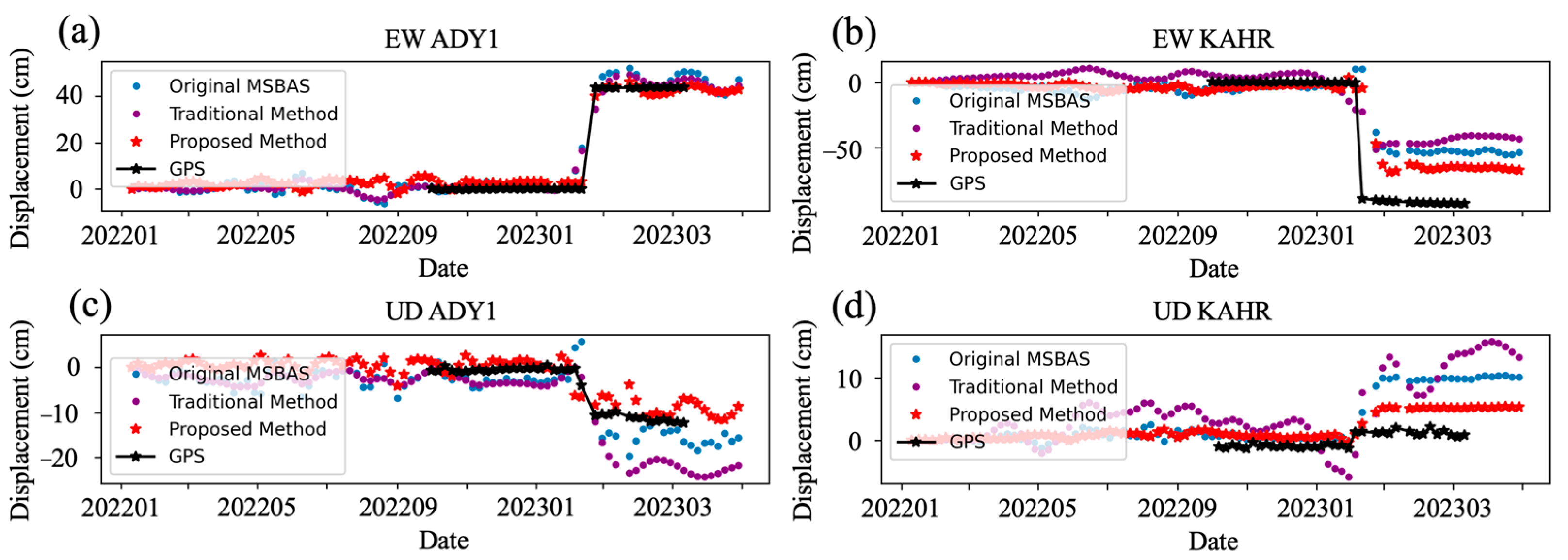
| Station | Direction | Original MSBAS STD (cm) | Traditional Method STD (cm) | Ratio | Proposed Method STD (cm) | Ratio |
|---|---|---|---|---|---|---|
| ADY1 | East–West | 0.0035 | 0.0031 | 10.94% | 0.0012 | 66.83% |
| ANTP | East–West | Ref | Ref | Ref | Ref | Ref |
| KAHR | East–West | 0.0224 | 0.0224 | 5.20% | 0.0172 | 23.29% |
| ADY1 | Up–Down | 0.0020 | 0.0019 | 4.95% | 0.0016 | 20.94% |
| ANTP | Up–Down | Ref | Ref | Ref | Ref | Ref |
| KAHR | Up–Down | 0.0036 | 0.0035 | 1.29% | 0.0013 | 61.25% |
Disclaimer/Publisher’s Note: The statements, opinions and data contained in all publications are solely those of the individual author(s) and contributor(s) and not of MDPI and/or the editor(s). MDPI and/or the editor(s) disclaim responsibility for any injury to people or property resulting from any ideas, methods, instructions or products referred to in the content. |
© 2024 by the authors. Licensee MDPI, Basel, Switzerland. This article is an open access article distributed under the terms and conditions of the Creative Commons Attribution (CC BY) license (https://creativecommons.org/licenses/by/4.0/).
Share and Cite
Liu, Y.; Wu, S.; Zhang, B.; Xiong, S.; Wang, C. Accurate Deformation Retrieval of the 2023 Turkey–Syria Earthquakes Using Multi-Track InSAR Data and a Spatio-Temporal Correlation Analysis with the ICA Method. Remote Sens. 2024, 16, 3139. https://doi.org/10.3390/rs16173139
Liu Y, Wu S, Zhang B, Xiong S, Wang C. Accurate Deformation Retrieval of the 2023 Turkey–Syria Earthquakes Using Multi-Track InSAR Data and a Spatio-Temporal Correlation Analysis with the ICA Method. Remote Sensing. 2024; 16(17):3139. https://doi.org/10.3390/rs16173139
Chicago/Turabian StyleLiu, Yuhao, Songbo Wu, Bochen Zhang, Siting Xiong, and Chisheng Wang. 2024. "Accurate Deformation Retrieval of the 2023 Turkey–Syria Earthquakes Using Multi-Track InSAR Data and a Spatio-Temporal Correlation Analysis with the ICA Method" Remote Sensing 16, no. 17: 3139. https://doi.org/10.3390/rs16173139
APA StyleLiu, Y., Wu, S., Zhang, B., Xiong, S., & Wang, C. (2024). Accurate Deformation Retrieval of the 2023 Turkey–Syria Earthquakes Using Multi-Track InSAR Data and a Spatio-Temporal Correlation Analysis with the ICA Method. Remote Sensing, 16(17), 3139. https://doi.org/10.3390/rs16173139