Trade-Off and Synergy Relationships and Driving Factor Analysis of Ecosystem Services in the Hexi Region

Abstract

The Hexi region, located in a sensitive and fragile ecological zone in northwest China, requires a scientific assessment of ecosystem services and their interactions. Identifying the main factors influencing spatial distribution is crucial for the sustainable development and effective management of the region. This study evaluates key ecosystem services, including regulating services (water conservation, soil conservation, carbon storage) and provisioning services (NPP), using Spearman’s correlation and pixel-by-pixel spatial analysis to calculate spatial trade-offs and synergies. Geographic detectors were used to uncover the underlying driving mechanisms. The results show that: (1) From 2000 to 2020, soil conservation, NPP, and carbon storage showed fluctuating growth, while water conservation declined. Spatially, high-value areas of water conservation, carbon storage, and NPP were concentrated in the central and southern areas, while high values of soil conservation services were mainly in the northwest and southeast regions. (2) The trade-offs and synergies among various ecosystem services exhibit temporal shifts, along with spatial scale effects and heterogeneity. In the study area, the proportion of pixels showing a trade-off relationship between water conservation and soil conservation, and between water conservation and NPP, accounts for 48.21% and 21.42%, respectively. These trade-offs are mainly concentrated in the central and southeastern regions, while the northwestern counties predominantly exhibit synergies. (3) Precipitation was the dominant factor for water conservation, carbon storage, and NPP, as well as for the trade-offs among these services. Among natural factors, climatic factors were significantly more influential than socio-economic factors, and the interaction between two factors had a greater explanatory power than single factors.

1. Introduction

Ecosystems provide a variety of services through complex ecological processes, such as food supply, soil conservation, and water conservation. These services result from human utilization of ecosystems and reflect their role in supporting human well-being [1]. As a bridge connecting nature and society, ecosystem services are generally categorized into four main types: provisioning services, regulating services, supporting services, and cultural services, which form the foundation for the sustainable development of human society [2].

Ecosystems are dynamic and continuous, thus quantifying ecosystem services at a single point in time and space is not sufficiently comprehensive. Quantifying, analyzing, and assessing ecosystem services using long-term data supports effective ecological protection and restoration management decisions. Recently, the rapid development of remote-sensing satellite technology and cloud-computing platforms has allowed researchers to focus on using long-term data to evaluate ecosystem changes [3,4,5]. This method has been widely applied to various ecosystems, such as urban areas [6,7,8], farmlands [9,10], and oceans [11,12], as well as to different scales, including counties [13], watersheds [14], and on a global level [15]. Additionally, handling different time scales, such as seasons [16], years, or longer periods [17], has become more efficient with remote-sensing and cloud-computing platforms. This allows for the quantitative inversion of dynamic changes in ecosystem characteristics, revealing underlying driving mechanisms, and facilitating cross-regional and cross-scale analyses [18]. Recently, the study of trade-offs and synergies between ecosystem services (ESs) has gained attention and has been applied to management decisions [19,20]. Research mainly focus on cities [21], ecological functional zones [22], and typical watersheds [23], while studies on specific climatic regions are relatively few. Methodologically, some studies use Spearman correlation and partial correlation analyses to identify trade-offs and synergies between different ESs [24,25,26]. However, the relationships between ecosystem services are complex and often influenced by temporal and spatial factors, making it difficult to accurately characterize their overall status and evolution. Some studies utilize Matlab or R programming languages to identify and quantitatively characterize the spatial trade-offs and synergies of ESs, overcoming the limitations of previous methods and better representing their spatial distributions [27,28]. Changes in ESs result from the combined effects of multiple factors, and identifying the key factors influencing these changes is fundamental for subsequent spatial management and ecosystem restoration efforts. Currently, models like geographically weighted regression and XGBoost are used to identify driving factors [14], but these methods have issues with regression assumptions and variable collinearity or are considered black-box models, making it difficult to explain the reasoning process behind them [29]. Many phenomena in physical geography exhibit spatial autocorrelation and heterogeneity. The Geodetector is highly sensitive to measuring the spatial differentiation of variables and detecting factors. They are more flexible in exploring non-linear relationships than traditional linear analysis methods and can better avoid endogeneity problems in regression analysis [30]. The Geodetector has unique advantages in addressing spatial heterogeneity. It can not only represent the explanatory power of single factors on the spatial differentiation of dependent variables but can also evaluate the interaction types when two factors work together. This helps in understanding the response of ecosystems and their services to driving factors [31,32]. In conclusion, effectively utilizing long-term remote-sensing data to assess regional ecosystem services and their underlying driving mechanisms provides strong theoretical support for governments and policymakers in their interventions.

The Hexi region, located in the arid and semi-arid inland areas of northwest China, includes diverse landscapes and functional types, such as the Qilian Mountains’ water conservation priority ecological function zone and typical desert areas, making the ecological environment sensitive and fragile. Under the backdrop of the Western Development Strategy and the Belt and Road Initiative, intense human activities have introduced new challenges to the sustainable development of the region’s ecological environment [33]. Currently, most studies on ecosystem services in the Hexi region focus on single services or are limited to evaluations within nature reserves, lacking systematic assessments at the county scale of multiple ecosystem services and the driving factors behind their interactions, particularly in typical desert ecological restoration areas [34,35]. Therefore, this study addresses the region’s water scarcity and desertification issues by focusing on regulating services, specifically water conservation and soil conservation. Additionally, in the context of carbon neutrality, carbon storage is included as an indicator of carbon sequestration under regulating services. Net Primary Productivity (NPP) is also considered an indicator that directly reflects the ecosystem’s provisioning capacity. Based on this, the Geodetector model is employed to analyze the dominant factors influencing ecosystem services within the study area, aiming to provide management support and practical guidance for the sustainable development of ecosystems. This study aims to provide a theoretical basis for the assessment and management of the ecological environment in the Hexi region and similar ecologically fragile areas. The specific objectives are (1) to quantitatively evaluate the spatiotemporal evolution characteristics of ecosystem services in the Hexi region; (2) to elucidate the spatiotemporal characteristics of trade-offs and synergies of ecosystem services in the Hexi region at different scales; and (3) to identify the dominant factors influencing the spatial distribution of services and their trade-offs and synergies.

2. Materials and Methods

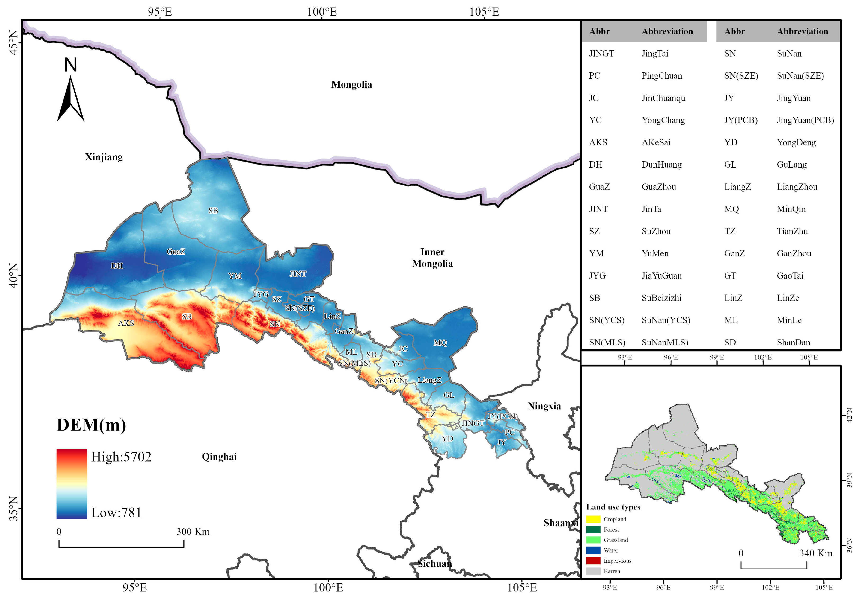
2.1. Study Area

The study area includes the desert ecological protection and restoration zone of the Hexi Corridor and the Qilian Mountain ecological protection zone, covering Wuwei, Jinchang, Zhangye, Jiuquan, Jiayuguan, Lanzhou, and Baiyin, totaling 24 districts and counties across 7 cities (Figure 1). Located in the northwest of Gansu Province and to the west of the Yellow River, the study area is bounded by Wushaoling to the east and Yumenshan to the west, with terrain sloping from the southwest to the northeast. It contains the Tengger and Badain Jaran Deserts and the inland river systems of the Heihe, Shule, and Shiyang Rivers, which nourish the oases. The region has a typical temperate continental climate, with annual precipitation ranging from 35 to 500 mm, an average annual temperature of 5.8 to 9.3 °C, and evaporation exceeding 1500 mm in most areas [36,37]. The main soil types are brown desert soil, gray–brown desert soil, gray desert soil, and gray–calcic soil [38]. Vegetation primarily includes grasslands, farmland, and forests, with the Qilian Mountains showing clear vertical distribution of vegetation from 2000 m upwards, consisting of desert steppe, steppe, forest steppe, shrub steppe, meadow steppe, and alpine snow zones. Due to its unique geographical location, the region serves as both a national ecological security barrier and an economic transportation hub. Due to its unique geographical location, the region serves as both a national ecological security barrier and an economic transportation hub [39]. Therefore, there is an urgent need to assess ecosystem services in this region and optimize regional management to achieve sustainable ecological, economic, and social development.

2.2. Data Sources

This study relies primarily on a multi-source dataset to assess ecosystem service functions, their inter-relationships, and the identification of driving factors. The dataset includes digital elevation models (DEM), population data from LandScan, land use data, vegetation type data, soil data, meteorological data, and socio-economic data collected and processed through the Google Earth Engine (GEE) and other public data platforms (

Table 1. Summary of the primary data.

Data Type	Data Format	Resolution	Data Description and Source
DEM	tif	30 m	NASA SRTM Digital Elevation (https://earthengine.google.com/ accessed on 20 December 2023)
Land use\land cover	tif	30 m/year	Annual land cover dataset (https://zenodo.org/records/8176941 accessed on 20 December 2023)
NPP	tif	500 m/year	the MODIS MOD17A3 dataset (https://earthengine.google.com/ accessed on 20 December 2023)
Vegetational type	shp	/	China vegetation map (scale: 1:1,000,000) Resource and Environment Science and Data Center (https://www.resdc.cn/ accessed on 20 December 2023)
Gross domestic product (GDP)	tif	1 km/year	China GDP Spatial Distribution Grid Dataset Resource and Environment Science and Data Center (https://www.resdc.cn/ accessed on 20 December 2023)
Precipitation	tif	1 km/Month	1 km Resolution Monthly Potential Evapotranspiration Dataset, 1 km Resolution Monthly Average Temperature Dataset, 1 km Resolution Monthly Precipitation Dataset. Loess Plateau SubCenter, National Earth System Science Data Center, National Science and Technology Infrastructure of China (http://loess.geodata.cn accessed on 20 December 2023)
Potential evapotranspiration	tif	1 km/Month
Temperature	tif	1 km/Month
Population density	tif	1 km/year	Oak Ridge National Laboratory (https://landscan.ornl.gov accessed on 20 December 2023)
Soil data	tif	1 km	Harmonized World Soil Database, HWSD (https://www.fao.org/home/en/ accessed on 20 December 2023)
Human Footprint	tif	1 km/year	Human Footprint dataset (https://doi.org/10.1038/s41597-022-01284-8 accessed on 20 December 2023)

). All raster data types are uniformly projected and have consistent spatial resolutions.

2.3. Methods

2.3.1. Quantification of Ecosystem Service Functions

This study primarily quantifies four main ecosystem service functions during the period from 2000 to 2020: provisioning services (Net primary productivity—NPP), regulating services (water conservation, soil conservation, and carbon storage). It selects data from five time points: 2000, 2005, 2010, 2015, and 2020, to characterize changes in ecosystem service status in the Hexi region (

Table 2. Overview of ecosystem service assessment method.

Ecosystem Service	Type	Equation	Description
Provisioning Services	Net primary productivity (NPP)	$\mathrm{N}\mathrm{P}\mathrm{P}(\mathrm{x},\mathrm{t})=\mathrm{A}\mathrm{P}\mathrm{A}\mathrm{R}(\mathrm{x},\mathrm{t})\times \mathcal{E}(\mathrm{x},\mathrm{t})$	Net primary productivity (NPP) directly reflects the supply capacity of the ecosystem and can be used as an indicator for quantifying provisioning service directly [40]. In this context, APAR(x,t) and ε(x,t) represent the absorbed photosynthetically active radiation (MJ·m−2)and the actual light use efficiency (g·MJ−1) at time t, respectively [41].
Regulating Services	Soil conservation (SC)	$S_s=\mathrm{R}\mathrm{K}\mathrm{L}\mathrm{S}-\mathrm{U}\mathrm{S}\mathrm{L}\mathrm{E}=\mathrm{R}\times \mathrm{K}\times \mathrm{L}\mathrm{S}-\mathrm{R}\times \mathrm{K}\times \mathrm{L}\mathrm{S}\times \mathrm{C}\times \mathrm{P}$	This study applies the Revised Universal Soil Loss Equation (RUSLE) to calculate soil conservation [42]. Ss represents the soil conservation amount (t/hm2) of grid cell s. R is the rainfall erosivity factor, which is calculated based on the average monthly and annual rainfall amounts [43]; K is the soil erodibility factor, which was determined using the nomograph method [44]; L is the slope length factor; and S is the slope steepness factor, both of which were calculated using the formulas provided in the Revised Universal Soil Loss Equation (RUSLE) [45]. C and P are the vegetation cover and management factor and the soil conservation practice factor, respectively [46,47].
	Water conservation (WC)	$\mathrm{W}\mathrm{C}={\displaystyle \sum _{\mathrm{i}=1}^{\mathrm{j}}} \left({\mathrm{P}}_{\mathrm{i}}-{\mathrm{R}}_{\mathrm{i}}-\mathrm{E}{\mathrm{T}}_{\mathrm{i}}\right)\times {\mathrm{A}}_{\mathrm{i}}\times {10}^3$	This study used the water balance equation to calculate water conservation capacity [48]. WC represents the water conservation capacity (m3), Pi is the rainfall (mm), Ri is the surface runoff (mm), ETi is the evapotranspiration (mm), Ai is the area of the i-th type of ecosystem (km2), and i denotes the i-th type of ecosystem in the region. j represents the number of ecosystem types within the study area [49,50].
	Carbon stock (CS)	${\mathrm{S}}_{\mathrm{c}}={\mathrm{C}}_{\mathrm{a}\mathrm{b}\mathrm{o}\mathrm{v}\mathrm{e}}+{\mathrm{C}}_{\mathrm{b}\mathrm{e}\mathrm{l}\mathrm{o}\mathrm{w}}+{\mathrm{C}}_{\mathrm{s}\mathrm{o}\mathrm{i}\mathrm{l}}+{\mathrm{C}}_{\mathrm{d}\mathrm{e}\mathrm{a}\mathrm{d}}$	The calculation of carbon storage is based on the carbon module in the INVEST model [51]. Sc represents the total carbon storage, Cabove is the carbon in aboveground biomass, Cbelow is the carbon in belowground biomass, Csoil is the carbon in the soil, and Cdead is the carbon in the litter layer.

).

2.3.2. Trend Analysis

This study employs the Mann–Kendall (MK) test to analyze the trends in ecosystem services. The MK test is a widely used non-parametric method for detecting trend changes in time series data. Its advantages include not requiring assumptions about the data distribution and being suitable for various types of trend changes, including linear, non-linear, and periodic trends [52,53]. The formula is as follows:

$$\beta =\mathrm{mean}\left({\displaystyle \frac{x_j-x_i}{j-i}}\right),\forall \mathrm{j}>\mathrm{I}$$

(1)

where x_j and x_i are the time series data, and β denotes the slope value. A β greater than 0 indicates an increasing trend, while a β less than 0 indicates a decreasing trend. Based on the trend changes and significance, the results are classified into five levels: significant decrease, slight decrease, stable, slight increase, and significant increase.

2.3.3. Analysis of ESs Trade-Offs/Synergies

This study employs the Spearman correlation coefficient to measure the trade-off/synergy relationships of ecosystem services. The formula is as follows:

$$R(a,b)=1-{\displaystyle \frac{6\sum d_{ab}^2}{n^3-n}}$$

(2)

$$t=R\times \sqrt{{\displaystyle \frac{n-2}{1-R^2}}}$$

(3)

where $a$ and $b$ represent different categories of ecosystem services (ES); $R(a,b)$ represents the correlation coefficient between $a$ and $b$; $d_{ab}$ denotes the rank difference between a and $b$; n is the number of samples; t is the test value. When $R(a,b)$ > 0, it indicates a positive correlation between $a$ and $b$, representing synergy among ESs, with larger values indicating stronger synergy. Conversely, when $R(a,b)$ < 0, it indicates a negative correlation between $a$ and $b$, representing a trade-off among ESs, with smaller values indicating stronger trade-offs. Furthermore, based on the long-term changes in ecosystem services, the pixel-by-pixel spatial analysis method is used to calculate the correlation coefficients between pairs of ecosystem services within each grid to determine the spatial trade-off and synergy relationships. Therefore, using pixel-by-pixel spatial analysis to calculate spatial trade-offs and synergies in long-term change data can further enhance the study of overall trade-offs and synergies. The classification standards are presented in

Table 3. Judgment method of balancing synergy relationship.

Intensity of Trade-Off and Synergy Relationships	Basis for Determination
Strong Synergy	r > 0, p < 0.01
Medium Synergy	r > 0, 0.01 < p < 0.05
Weak Synergy	r > 0, 0.05 < p < 0.1
Independent	p > 0.1
Weak Trade-off	r < 0, p < 0.0
Medium Trade-off	r < 0, 0.01 < p < 0.05
Strong Trade-off	r < 0, 0.05 < p < 0.1

[32].

2.3.4. Analysis of Factors Influencing ESs and Their Trade-Offs and Synergies

This article employs the Geodetector to identify the primary driving factors behind ecosystems and their inter-relationships. The Geodetector is a suite of novel statistical methods designed to probe spatial heterogeneity and reveal the underlying forces driving such patterns. Its theoretical nucleus revolves around partitioning variables into multiple subregions, juxtaposing the spatial variance within each subregion with those between different subregions, thereby ascertaining the explanatory power of multiple independent variables on the dependent variable. This approach facilitates the discernment of key drivers shaping complex ecological systems and their spatial variations [30].

Single Factor Detection: This process involves comparing the total variance of the study area with the sum of variances across the subregions obtained after classification, to investigate the spatial disparity of attribute Y, or to what extent a factor X explains the spatial disparity of Y. This is quantified using the q statistic, expressed as follows:

$$\begin{array}{c}q=1-{\displaystyle \frac{\sum _{h=1}^L N_h{\sigma }_h^2}{N{\sigma }^2}}\end{array}$$

(4)

where h = 1, …, and L signifies the stratification levels of variable Y or factor X, indicative of classification or zoning; $N_h$ and $N$ denote the counts of units within layer h and the overall study area, respectively; ${\sigma }^2$ and ${ \sigma }_h^2$ are the variances of Y values computed for the entire study area and each individual layer $h$. The metric $q$ spans from 0 to 1, with larger values implying a heightened degree of spatial differentiation in Y or an augmented explanatory power of X over the spatial disparities exhibited by Y.

Interactive Detection: The Geodetector is capable of examining the combined explanatory capacity of two distinct factors on the spatial differentiation of variable Y when they act concurrently. This interactive effect can manifest as a multiplicative relationship or any other form of composite interaction. Types of interactive effects are categorized into non-linear attenuation, single-factor non-linear attenuation, dual-factor amplification, independence, and non-linear enhancement.

3. Results

3.1. Spatial and Temporal Distribution Characteristics of Ecosystem Service Functions

By selecting data from five periods between 2000 and 2020 and corresponding trend change charts, it was found that the spatial and temporal distribution characteristics of various ecosystem service functions in the study area have changed significantly (Figure 2). Over the 20 years, the water conservation capacity per unit area of the entire region decreased annually, from 244.9 m³/hm² in 2000 to 63.9 m³/hm² in 2020. Compared to other periods, the decline in water conservation capacity was most significant between 2000 and 2005, reaching 58.43%. Spatially, the eastern part of the study area mainly showed a decreasing trend, while scattered areas in the west showed a slight increase. The range of high-value areas initially contracted and then slowly expanded. Minle County and Shandan County in the central part of the study area were the main high-value aggregation areas in the later period, with average water conservation capacities of 16.2 m³/hm² and 17.7 m³/hm², respectively, in 2020.

Soil conservation services showed fluctuating growth, reflecting the overall soil conservation capacity increasing from 6.59 t/hm² in 2000 to 11.89 t/hm² in 2020, with an average change rate of 33.19% every five years. Jingyuan County in the southeast saw the highest increase, with the soil conservation capacity rising from 17.83 t/hm² in 2000 to 42.46 t/hm² in 2020. Spatially, high values were mainly concentrated in the flat areas around the northern foothills of the Qilian Mountains and the southeastern region, with the center of these high-value areas gradually shifting from northwest to southeast and the range expanding. There was also a significant difference in soil retention values between the northern and southern sides of the Qilian Mountains, with the north-south variation trend being particularly pronounced in central Su’nan County.

The average annual NPP in the study area was 55.88 gC/m², with an average increase of 8.49% every five years. The spatial distribution showed a clear clustering characteristic, with high-value areas in the northern foothills of the Qilian Mountains and nearby regions, and the range gradually expanding. The spatial trend was mainly increasing, while in highly urbanized areas, such as Liangzhou District and Ganzhou District, the NPP exhibited a significant decreasing trend.

Carbon storage remained relatively stable from 2000 to 2020, averaging 54.78 t/hm². Its spatial distribution was mainly influenced by land use types, with high-value areas primarily distributed in grasslands and forests. The growth trend accounted for 40.04% of the total grassland area, primarily concentrated in the northwestern grassland types, while in impermeable surfaces, the trend was predominantly decreasing, accounting for 43.80% of the total area.

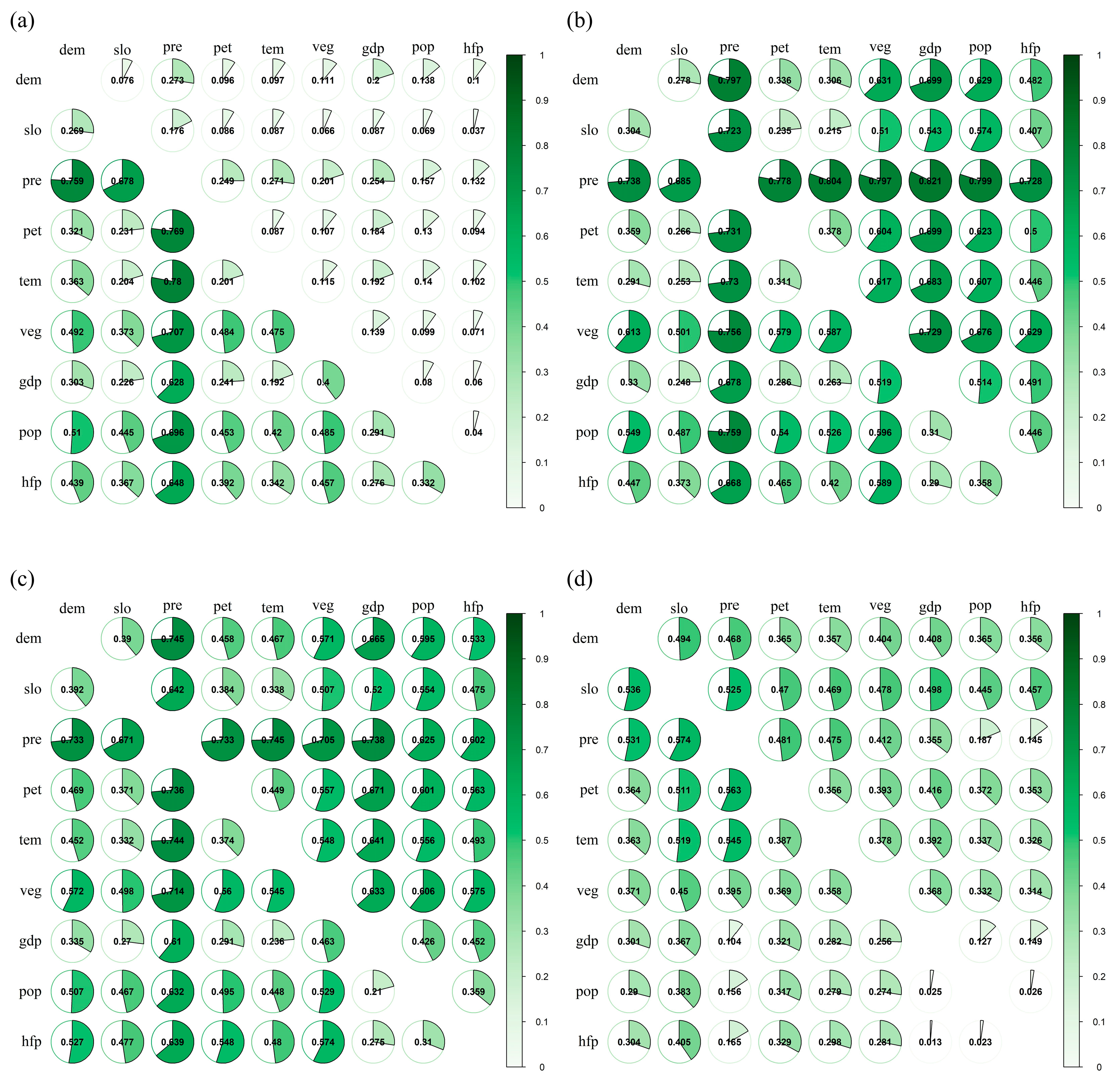
3.2. Analysis of Trade-Off and Synergy Relationships

Through the analysis of data from 2000 to 2020, this study found a total of six statistically significant correlations (p < 0.001) among the four ecosystem services (Figure 3). At the regional scale, carbon storage is positively correlated with soil conservation and NPP, with the former showing a fluctuating upward trend, and the latter showing a fluctuating downward trend in correlation coefficients. In 2002, the relationship between water conservation and carbon storage shifted from synergy to trade-off, with the correlation coefficient continuously decreasing, indicating a strengthening trade-off relationship. The relationships between water conservation and NPP, and between water conservation and soil conservation, fluctuate between trade-off and synergy from year to year, with significant variability. In 2020, these relationships, respectively, showed synergy and trade-off. The relationship between NPP and soil conservation was consistently a trade-off throughout the study period, although the strength of this trade-off relationship gradually weakened over time.

Employing spatial pixel-by-pixel analysis on long-term time-series data, we explored the trade-offs and synergies among the four key ecosystem services, uncovering significant spatial heterogeneity in these relationships (Figure 3). The relationships between carbon storage and NPP, water conservation, soil conservation, and the relationship between NPP and soil conservation, were primarily synergistic. The proportions of pixels showing synergistic relationships were 33.22%, 22.05%, 22.12%, and 34.01%, respectively. The synergy between soil conservation and NPP showed a clustering phenomenon, mainly distributed in the northern foothills of the Qilian Mountains and the southeastern part of the study area. The synergistic relationships of carbon storage with NPP, water conservation, and soil conservation exhibited spatial consistency, mainly concentrated in Zhangye City and its surrounding areas in the central part of the study area. Within the study area, the relationships between water conservation and NPP, and between water conservation and soil conservation, were predominantly trade-offs, showing clustering characteristics, with pixel proportions of 21.42% and 48.21%, respectively. The trade-off relationship with NPP was mainly distributed in the central part of the study area, while the trade-off relationship between water conservation and soil conservation was mainly concentrated in the southeastern part of the study area.

Based on the above data, a statistical analysis at the district and county level was conducted (Figure 4). The results showed that the relationship between carbon storage and NPP was predominantly synergistic in most districts and counties. However, in certain areas, such as Guazhou County, Jinta County, Yumen City in the north of the study area and Yongdeng County in the southeast, the proportion of pixels showing a trade-off relationship exceeded those showing a synergistic relationship, with percentages of 52.40%, 46.67%, 43.86%, and 44.53%, respectively. The relationship between carbon storage and water conservation was predominantly a trade-off in Jingyuan County, Pingchuan District, Yongdeng County in the southeast, and Liangzhou District in the central part of the study area, consistent with the overall regional trend. In Yongdeng County, the relationship between carbon storage and soil conservation deviated from the overall pattern, with strong and medium trade-off pixels accounting for 11.82% and 13.49%, respectively, indicating a notable conflict between these two services. The relationship between NPP and soil conservation at the district and county level was generally consistent with the overall regional trend, being predominantly synergistic, with strong synergy pixels exceeding 30% in Jinchuan District, Yongchang County, and Su’nan District in the central part of the study area. The relationship between NPP and water conservation was predominantly synergistic in Jingtai County in the southeast, Aksai District, and Yumen City in the north, differing from the overall pattern. The trade-off between water conservation and soil conservation is particularly pronounced in the southeastern regions, such as Jingtai County, Jingyuan County, and Pingchuan District, where the average proportions of pixels showing medium and strong trade-off are 22.21% and 61.81%, respectively. In contrast, in northern Jinta County, the number of pixels exhibiting a synergistic relationship slightly exceeds those showing a trade-off, accounting for 33.82%.

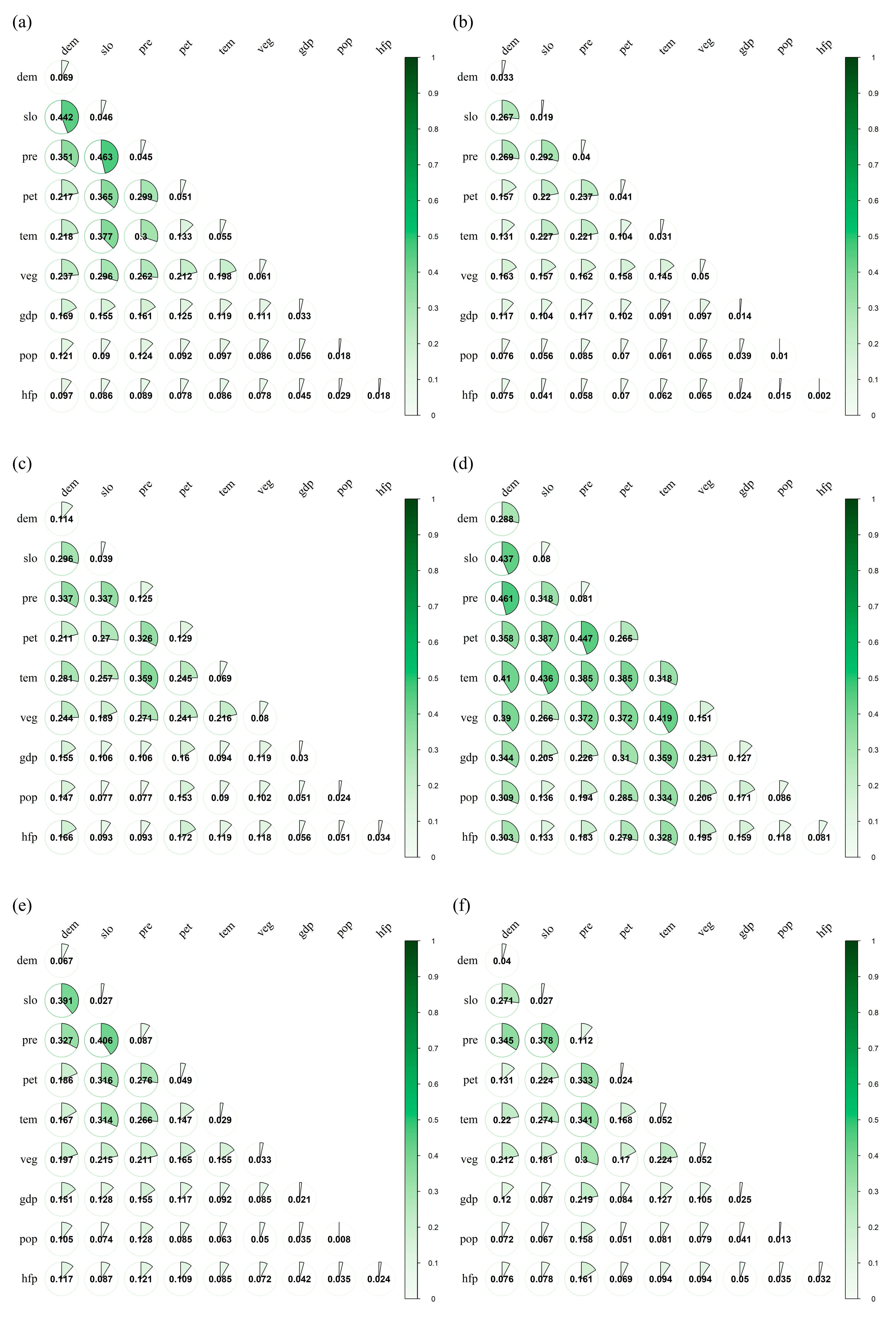
3.3. Analysis of Influencing Factors

Spatial variations in ecosystem services are influenced by a combination of geographical conditions, climate, and socioeconomic factors. The factor exploration results indicate that precipitation is the dominant factor for water conservation, carbon storage, and NPP, followed by potential evapotranspiration, population density, and vegetation type (

Table 4. Single-factor detection results of ecosystem service functions.

	WC		NPP		SC		CS
	2000	2020	2000	2020	2000	2020	2000	2020
DEM	0.176	0.046	0.182	0.190	0.275	0.329	0.254	0.273
SLO	0.088	0.012	0.097	0.085	0.355	0.407	0.198	0.214
PRE	0.568	0.112	0.598	0.682	0.067	0.075	0.586	0.563
PET	0.094	0.051	0.135	0.145	0.304	0.332	0.203	0.241
TEM	0.048	0.054	0.102	0.102	0.268	0.299	0.137	0.164
VEG	0.299	0.044	0.465	0.482	0.248	0.281	0.438	0.451
GDP	0.101	0.042	0.116	0.331	0.006	0.107	0.061	0.271
POP	0.258	0.029	0.283	0.381	0.021	0.019	0.199	0.293
HFP	0.233	0.021	0.249	0.303	0.009	0.007	0.264	0.268

Note: DEM stands for elevation; SLO stands for slope; PRE stands for annual precipitation; PET stands for annual evaporation; TEM represents the average annual temperature; VEG stands for vegetation type; GDP stands for gross domestic product; POP stands for population density; HFP stands for human footprint.

). Specifically, the q-value for carbon storage shows a slight decrease, while for water conservation, it significantly drops from 0.568 in 2000 to 0.112 in 2020. Conversely, the q-value for NPP increases from 0.598 in 2000 to 0.682 in 2020. Slope is identified as the primary factor influencing soil conservation services, with its q-value increasing from 0.355 in 2000 to 0.407 in 2020, followed by potential evapotranspiration and digital elevation model (DEM), while socio-economic factors have a weaker influence. In the results of the detection of interactive factors (Figure 5), we found that precipitation, as the dominant factor for water conservation, carbon storage, and NPP (net primary productivity), remains the most important interactive factor within the region. Specifically, for water conservation, the dominant influencing factors in both 2000 and 2020 were precipitation interacting with temperature, followed by interactions with potential evapotranspiration, DEM (digital elevation model), and other factors. For NPP, the dominant influencing factors in 2000 and 2020 were precipitation interacting with vegetation type and GDP (gross domestic product), with q-values of 0.76 and 0.82, respectively, indicating that climate conditions, vegetation conditions, and socio-economic factors have a significant spatial impact on NPP. For carbon storage, interactions between precipitation and potential evapotranspiration, as well as temperature, were the primary factors influencing its distribution in 2000 and 2020, followed by interactions with DEM and vegetation type. Furthermore, in factor detection, slope had the greatest explanatory power for soil conservation services. Therefore, in interaction detection, the interaction between slope and precipitation emerged as the dominant factor influencing soil conservation services. Secondary factors shifted from the interaction between precipitation and temperature in 2000 to the interaction between slope and GDP in 2020, indicating a shift from purely natural factors to the combined influence of natural and socio-economic factors affecting the spatial distribution of soil conservation services.

On the other hand, using the multi-year average of dependent variables as the influencing factor for spatial heterogeneity in ecosystem service relationships, we analyzed the dominant factors affecting the spatial distribution of balanced synergistic relationships (Figure 6). The results revealed that precipitation is a primary factor influencing the balanced synergistic distribution between water conservation, carbon storage, and NPP (net primary productivity), with DEM (digital elevation model) and temperature following. For the balanced synergistic relationship between soil conservation and water conservation, potential evapotranspiration and precipitation were the main influencing factors, with q-values of 0.13 and 0.12, indicating that climate conditions have a significant impact compared to other factors. Temperature was found to be the main factor influencing the relationship between soil conservation and NPP, with a q-value of 0.32. Vegetation type emerged as the primary factor influencing the distribution of soil conservation and carbon storage. DEM and vegetation type were also identified as the main driving factors for carbon storage and NPP. Compared to factor detection, the explanatory power of each factor for the spatial distribution of ecosystem services with balanced synergistic relationships was significantly enhanced under interaction. Specifically, for the balanced synergistic relationships between water conservation and carbon storage, NPP, and soil conservation with NPP, the main interactive factors aligned with their corresponding single-factor-dominant factors, showing enhanced dual-factor and non-linear effects with q-values of 0.41, 0.47, and 0.38, respectively. In contrast, for other relationships, the dominant factors between single-factor and interactive factors changed, such as between carbon storage and NPP, soil conservation, and soil conservation with water conservation.

4. Discussion

Currently, cloud-computing platforms like GEE enable rapid access to diverse ecological data elements, offering efficient data-processing capabilities and abundant remote-sensing resources. This makes large-scale spatiotemporal analysis feasible and enhances the capabilities for regional assessment and monitoring. Therefore, this study utilizes long-term data to analyze ecosystem service characteristics, providing a macroscopic evaluation of ecological conditions in the study area from 2000 to 2020. It quantifies the main ecosystem services and their interactions and identifies the primary driving factors of their spatial distribution using Geodetector. The results reveal significant interannual fluctuations in the four ecosystem services within the study area. Soil conservation, net primary productivity (NPP), and carbon storage have all shown improvements, whereas water conservation services exhibit a declining trend. This finding aligns with conclusions drawn from studies on ecosystem services in arid regions during the same period [35,54]. There is evident spatial heterogeneity among these services. On one hand, the region’s high evapotranspiration capacity relative to precipitation, coupled with human activities altering surface energy balance and permeability, affects local water circulation, groundwater recharge, and runoff generation, thereby decreasing overall water conservation capacity [55,56,57]. On the other hand, due to “warm–humid” conditions and glacier meltwater contributions, water storage in the northern Shule River and Heihe River basins has increased, resulting in improved local water conservation services [58,59]. Except for unused land, the northern region is dominated by grasslands, with steep slopes in mountainous areas leading to severe soil erosion and generally lower soil conservation and carbon storage [60]. In contrast, the plains in the northern part have fertile soils and sufficient water, resulting in higher carbon storage and NPP. In the relatively moderate plains of the central and southern regions, improvements in soil conservation and NPP services are evident due to increased agricultural productivity and ecological engineering efforts such as vegetation restoration, showing a sustained increasing trend.

Natural factors and internal ecosystem regulation affect the interactions between ESs, but human factors such as land use changes and ecological protection policies also create complex trade-offs and synergies among ESs, leading to spatial heterogeneity and interannual variability [61]. The trade-offs and synergies between different ESs change over time but tend to stabilize over time. This is similar to our findings that the trade-offs and synergies between water conservation, NPP, and soil conservation fluctuate over time [62]. However, quantifying ES functions through a pixel-by-pixel approach might overlook the temporal details of ES trade-offs [63]. For instance, the overall spatial trade-offs and synergies between water conservation, NPP, and soil conservation are dominated by trade-offs, which do not align with the temporal fluctuations. Therefore, combining annual analysis and spatial quantification of ES trade-offs and synergies helps implement effective measures at different regional and temporal scales to optimize ES relationships. Based on this, further exploration of trade-offs and synergies at the county level reveals regional heterogeneity. We found significant differences in the predominant proportions of trade-offs and synergies at the spatial and regional levels. For example, carbon storage and water conservation mainly show synergies across the entire region (21.05%). However, in Pingchuan District (28.92%) and Jingyuan County (32.77%) in the southeast, trade-offs are evident. This is similar to findings in the Loess Hilly Region, likely due to severe soil erosion and local afforestation and grass-planting efforts, which increase vegetation and carbon sequestration, balancing each other out [64]. This indicates that when exploring the trade-offs and synergies of ecosystem services, it is essential not only to investigate changes in a single year but also to consider differences caused by spatial geographic locations. Moreover, it is crucial to strengthen the long-term monitoring of services across different land types. This approach will enable the development of targeted ecosystem protection management policies based on differences in overall and local characteristics, thereby maximizing the benefits and sustainability of ecosystem services.

Understanding the temporal and spatial changes in major ecosystem services in the study area and the driving factors behind their interactions is crucial for recognizing and optimizing trade-offs and synergies among these services. This study uses Geodetector to analyze the dominant factors affecting ecosystem services and their interactions. The results show that natural factors have a greater impact on ecosystem services and their trade-offs and synergies than socio-economic factors. Moreover, the interaction between any two driving factors enhances the explanatory power for the spatial differentiation of the dependent variable, which is consistent with previous studies [32]. For example, the main driving factors for NPP (a provisioning service) and water conservation (a regulating service) are similar, with precipitation being the primary factor. This is likely because rainfall is a limiting factor for vegetation growth and photosynthesis in arid regions [65]. Vegetation reduces soil evapotranspiration during growth, and its roots improve soil structure, stabilize soil, and enhance water conservation, significantly affecting water conservation [66,67,68]. When precipitation interacts with other factors, its explanatory power increases, indicating that single-factor explanations are limited and multi-factor interactions are more effective in evaluating impacts on ecosystem services. Therefore, future monitoring and policy-making should consider the combined effects of multiple factors to enhance scientific accuracy and effectiveness. Additionally, the calculation of carbon storage in this study relies on carbon density data from land use types, which are influenced by climate, vegetation type, topography, soil, and human activities [69]. Our findings are consistent with this. Studies have shown that high soil conservation values are found in low to mid-altitude, steep slopes, and semi-shaded areas [20], aligning with our results. Interaction detection reveals that precipitation and potential evapotranspiration are the main factors affecting its spatial distribution, likely due to their combined impact on soil moisture, soil structure, and plant growth, thus influencing soil conservation services [70,71]. Additionally, we found that, except for NPP and water conservation, the explanatory power of the interaction factors of natural elements for other services decreased to varying degrees in 2020 compared to 2000, while the explanatory power of interactions with socio-economic factors slightly increased. This may be related to recent ecological protection and restoration projects in the Hexi region, which have reduced the explanatory power of natural factors and increased the influence of human activities. For water conservation, the explanatory power of all single and interaction factors in 2020 was significantly lower than in 2000. This may be due to the higher sensitivity and lag in response to various influencing factors (natural and human) in water-scarce arid regions, reducing the overall explanatory power of each factor [72,73].

Net primary productivity (NPP), which serves as a provisioning service, and water conservation, a regulating service, share similar dominant drivers. Precipitation affects vegetation distribution, and different vegetation types’ varying water and nutrient requirements significantly influence the spatial distribution patterns of NPP [65]. Water conservation capacity depends primarily on the influence of precipitation and evapotranspiration, and changes in regional water cycling and human activities also lead to variations in service functions. The calculation of carbon storage relies on carbon density data of land use types, which are influenced by a combination of climate, vegetation type, terrain, soil, and human activities, consistent with the study’s findings. Studies have shown that soil conservation is highest in areas of medium to low altitude, steep slopes, and semi-shaded slopes [20], consistent with the results of this study. Additionally, interaction detection shows that precipitation and potential evapotranspiration are the main factors influencing their spatial distribution. This is likely because their interaction affects ecological processes such as soil moisture content, soil structure, and plant growth, thereby influencing soil conservation services [70,71].

When factor detection was conducted for trade-offs and synergies among services, the q-values of interaction factors were significantly higher than those of single factors, and the results for single and interaction factors were not completely consistent. For example, in detecting the trade-off and synergy relationship between soil conservation and carbon storage, the dominant factor in single-factor detection was vegetation type, while the interaction factor detection result was precipitation and slope. This indicates that vegetation growth may be influenced by both precipitation and slope, and the trade-off and synergy relationship between the two services is more significantly affected by the combined influence of these factors than by a single factor. Therefore, the Hexi region should adopt flexible adaptive management strategies in regulation, promptly respond to environmental changes and variations in factor influence, and formulate differentiated management measures based on the climate conditions and ecological characteristics of different areas.

This study still has some uncertainties and limitations. Remote sensing is an efficient means for monitoring and assessing at spatial scales, but due to data acquisition limitations and varying data sources, the accuracy of assessments is limited. During factor detection analysis, factor selection and regional differences may lead to incomplete explanations of the underlying driving mechanisms. Future research should further validate the accuracy of assessments and delve deeper into the differences in driving factors at different scales, tailoring ecological protection policies to local conditions by considering trade-offs and synergies among services.

5. Conclusions

This study uses the Hexi region as a case study to quantify the spatiotemporal changes in four ecosystem services, analyze the overall and local spatial distribution of trade-offs and synergies among these services, and reveal the dominant factors behind them using geographic detectors. The conclusions are as follows: (1) From 2000 to 2020, the spatiotemporal differences in ecosystem services (ESs) in the study area were significant. Over this period, soil conservation, NPP, and carbon storage exhibited fluctuating growth, while water conservation showed a declining trend. Spatially, high values of water conservation were mainly concentrated in the central and southern regions, whereas the northern region showed a relative increase. High values of NPP and carbon storage were mainly concentrated in the southern and central regions, showing an outward-expansion trend. Soil conservation services were higher in the northern Subei and southeastern areas, exhibiting a continuous increasing trend, while soil conservation in the Qilian Mountains region area showed a declining trend. (2) The ecosystem services exhibit dynamic trade-offs and synergies in both temporal and spatial dimensions. Temporally, the trade-offs and synergies among water conservation, NPP, carbon storage, and soil conservation services change annually. Spatially, there is heterogeneity across different scales. At the regional scale, water conservation mainly shows trade-offs with NPP and soil conservation, while other services are primarily synergistic. At the county scale, the trade-offs between NPP and soil conservation are sporadically distributed near Yongchang County. The synergies between water conservation and NPP are mainly found in Jingtai County and Yumen City, while the trade-offs between water conservation and soil conservation are primarily in southeastern areas such as Jingyuan County and Jingtai County. The trade-offs and synergies among carbon storage, NPP, soil conservation, and water conservation are consistently scattered. (3) Precipitation is the dominant factor for water conservation, carbon storage, and NPP, as well as for the interactions between water conservation and carbon storage and NPP. Slope is the dominant factor for soil conservation. Potential evapotranspiration is the dominant factor for both soil conservation and water conservation. Temperature is the dominant factor for both soil conservation and NPP. DEM and vegetation type are the dominant factors for carbon storage, NPP, and soil conservation, respectively.

References

1. Wang, D.; Zheng, H.; Ouyang, Z. Ecosystem Services Supply and Consumption and Their Relationships with Human Well-Being. Chin. J. Appl. Ecol. 2013, 24, 1747–1753. [Google Scholar] [CrossRef]
2. Millennium Ecosystem Assessment, MEA. Ecosystems and Human Well-Being; Island Press: Washington, DC, USA, 2005. [Google Scholar]
3. Cao, S.; Hu, X.; Wang, Y.; Chen, C.; Xu, D.; Bai, T. Understanding Spatial-Temporal Interactions of Ecosystem Services and Their Drivers in a Multi-Scale Perspective of Miluo Using Multi-Source Remote Sensing Data. Remote Sens. 2023, 15, 3479. [Google Scholar] [CrossRef]
4. White, H.J.; Gaul, W.; Sadykova, D.; León-Sánchez, L.; Caplat, P.; Emmerson, M.C.; Yearsley, J.M. Quantifying Large-scale Ecosystem Stability with Remote Sensing Data. Remote Sens. Ecol. Conserv. 2020, 6, 354–365. [Google Scholar] [CrossRef] [PubMed]
5. Wu, Q.; Yang, L.; Mi, J. Detecting the Effects of Opencast Mining on Ecosystem Services Value in Arid and Semi-Arid Areas Based on Time-Series Remote Sensing Images and Google Earth Engine (GEE). BMC Ecol. Evol. 2024, 24, 28. [Google Scholar] [CrossRef]
6. Wen, Y.; Yang, J.; Liao, W.; Xiao, J.; Yan, S. Refined Assessment of Space-Time Changes, Influencing Factors and Socio-Economic Impacts of the Terrestrial Ecosystem Quality: A Case Study of the GBA. J. Environ. Manag. 2023, 345, 118869. [Google Scholar] [CrossRef]
7. Li, G.; Wang, H.; Cao, Y.; Zhang, X.; Ning, X. Spatio-Temporal Evolution and Influencing Factors of Ecological Environment Quality in the Changsha-Zhuzhou-Xiangtan Urban Agglomeration. Remote Sens. Nat. Resour. 2023, 35, 244–254. [Google Scholar] [CrossRef]
8. Hao, J.; Wei, W.; Li, S.; Ma, M.; Li, X.; Yang, H.; Jiang, Q.; Chai, P. GEE Based Evaluation on Spatial-Temporal Pattern and Drivers of Long-Term Water Body in Beijing-Tianjin-Hebei. Ecol. Environ. Sci. 2023, 32, 556–566. [Google Scholar] [CrossRef]
9. Tian, F.; Zhang, Y.; Lu, S. Spatial-Temporal Dynamics of Cropland Ecosystem Water-Use Efficiency and the Responses to Agricultural Water Management in the Shiyang River Basin, Northwestern China. Agric. Water Manag. 2020, 237, 106176. [Google Scholar] [CrossRef]
10. Li, Y.; Zhang, Y.; Zhao, G.; Li, T.; Li, J.; Dou, J.; Fan, R. Remote Sensing Inversion and Application for Soil Fertility of Cultivated Land in the Hilly Areas of Central-South Shandong of China. Trans. CSAE 2020, 36, 269–278. [Google Scholar] [CrossRef]
11. Ping, B.; Meng, Y.; Xue, C.; Su, F. Oceanic Primary Production Estimation Based on Machine Learning. J. Geophys. Res. Ocean 2023, 128, e2022JC018980. [Google Scholar] [CrossRef]
12. Zheng, G.; Li, C. An Empirical Algorithm for Retrieving Chlorophyll-a Concentration in the Sea Area near Palawan Island. Sci. Surv. Mapp. 2022, 47, 168–176. [Google Scholar] [CrossRef]
13. Bi, Y.; Zheng, L.; Wang, Y.; Li, J.; Yang, H.; Zhang, B. Coupling Relationship between Urbanization and Water-Related Ecosystem Services in China’s Yangtze River Economic Belt and Its Socio-Ecological Driving Forces: A County-Level Perspective. Ecol. Indic. 2023, 146, 109871. [Google Scholar] [CrossRef]
14. Liu, Q.; Qiao, J.; Li, M.; Huang, M. Spatiotemporal Heterogeneity of Ecosystem Service Interactions and Their Drivers at Different Spatial Scales in the Yellow River Basin. Sci. Total Environ. 2024, 908, 168486. [Google Scholar] [CrossRef] [PubMed]
15. Peng, Y.; Chen, W.; Pan, S.; GU, T.; Zeng, J. Identifying the Driving Forces of Global Ecosystem Services Balance, 2000–2020. J. Clean. Prod. 2023, 426, 139019. [Google Scholar] [CrossRef]
16. Liu, S.; Zhang, H.; Pei, X.; Wang, Y. Drivers of Ecosystem Service Trade-off and Synergy in Long-Term Sequence: A Case Study of the Extremely Important Ecosystem Service Function Area in Wuhu City. Acta Ecol. Sin. 2024, 44, 1780–1790. [Google Scholar]
17. Shen, J.; Li, S.; Liu, L.; Liang, Z.; Wang, Y.; Wang, H.; Wu, S. Uncovering the Relationships between Ecosystem Services and Social-Ecological Drivers at Different Spatial Scales in the Beijing-Tianjin-Hebei Region. J. Clean. Prod. 2021, 290, 125193. [Google Scholar] [CrossRef]
18. Li, S.; Li, X.; Dou, H.; Dang, D.; Gong, J. Integrating Constraint Effects among Ecosystem Services and Drivers on Seasonal Scales into Management Practices. Ecol. Indic. 2021, 125, 107425. [Google Scholar] [CrossRef]
19. Anna, F. Cord; Bartosz Bartkowski; Michael Beckmann; Andreas Dittrich; Kathleen Hermans-Neumann; Andrea Kaim; Nele Lienhoop; Karla Locher-Krause; Jörg Priess; Christoph Schröter-Schlaack; et al. Towards Systematic Analyses of Ecosystem Service Trade-Offs and Synergies: Main Concepts, Methods and the Road Ahead. Ecosyst. Serv. 2017, 28, 264–272. [Google Scholar] [CrossRef]
20. Xue, Z.; Gao, Y.; Lu, P.; Zhou, J.; Wang, K.; Zhang, B.; Ma, Y.; Liu, M. Spatial Distribution and Tradeoff-Synergy-Independence Relationships of Ecosystem Services Based on Land Use and Topography. Res. Soil Water Conserv. 2024, 31, 240–251. [Google Scholar] [CrossRef]
21. Tian, P.; Liu, Y.; Li, J.; Pu, R.; Cao, L.; Zhang, H. Spatiotemporal Patterns of Urban Expansion and Trade-Offs and Synergies among Ecosystem Services in Urban Agglomerations of China. Ecol. Indic. 2023, 148, 110057. [Google Scholar] [CrossRef]
22. Li, Q.; Jia, Y.; Wanng, H.; Wang, Z. Analysis of Trade-off and Synergy Effects of Ecosystem Services in Hebei Province from the Perspective of Ecological Function Area. Acta Geogr. Sin. 2023, 78, 2833–2849. [Google Scholar]
23. Shen, J.; Zhao, M.; Tan, Z.; Zhu, L.; Guo, Y.; Li, Y.; Wu, C. Ecosystem Service Trade-Offs and Synergies Relationships and Their Driving Factor Analysis Based on the Bayesian Belief Network: A Case Study of the Yellow River Basin. Ecol. Indic. 2024, 163, 112070. [Google Scholar] [CrossRef]
24. Qiao, X.; Gu, Y.; Zou, C.; Wang, L.; Luo, J.; Huang, X. Trade-Offs and Synergies of Ecosystem Services in the Taihu Lake Basin of China. Chin. Geogr. Sci. 2018, 28, 86–99. [Google Scholar] [CrossRef]
25. Deng, Y.; Wang, D.; Xu, H. Trade-offs and Synergies Relationships of Ecosystem Services and Their Socio-ecological Driving Factors under Different Spatial Scales in Shaoguan City, Guangdong, China. Chin. J. Appl. Ecol. 2023, 34, 3073–3084. [Google Scholar]
26. Wang, P.; Zhang, L.; Li, Y.; Jiao, L.; Wang, H.; Yan, J.; Lv, Y.; Fu, B. Spatio-Temporal Characteristics of the Trade-off and Synergy Relationships among Multiple Ecosystem Services in the Upper Reaches of Hanjiang River Basin. Acta Geogr. Sin. 2017, 72, 2064–2078. [Google Scholar] [CrossRef]
27. Karimi, J.D.; Corstanje, R.; Harris, J.A. Bundling Ecosystem Services at a High Resolution in the UK: Trade-Offs and Synergies in Urban Landscapes. Landsc. Ecol. 2021, 36, 1817–1835. [Google Scholar] [CrossRef]
28. Liu, S. Effects of Landscape Pattern Change on Ecosystem Services and Its Interactions in Karst Cities: A Case Study of Guiyang City in China. Ecol. Indic. 2022, 145, 109646. [Google Scholar] [CrossRef]
29. Scowen, M.; Athanasiadis, I.N.; Bullock, J.M.; Eigenbrod, F.; Willcock, S. The Current and Future Uses of Machine Learning in Ecosystem Service Research. Sci. Total Environ. 2021, 799, 149263. [Google Scholar] [CrossRef]
30. Wang, J.; Xu, C. Geodetector: Principle and Prospective. Acta Geogr. Sin. 2017, 72, 116–134. [Google Scholar] [CrossRef]
31. Li, L.; Zhao, F.; Zhu, L.; He, S.; Ye, L. Geographical detection of ecosystem services trade-offs and their spatial variation mechanism in Qihe River Basin. Acta Ecol. Sin. 2021, 41, 7568–7578. [Google Scholar] [CrossRef]
32. Zhang, Z.; Zhang, L.; Sun, G.; Liu, J. Spatial and temporal effect and driving factors of ecosystem service trade-off in the Qingjiang River Basin, China. Chin. J. Appl. Ecol. 2023, 34, 1051–1062. [Google Scholar] [CrossRef]
33. Yang, L.; Yang, H.; Yang, Y.; Wei, W.; Pan, J. Spatial-temporal evolution of ecological environment quality in Hexi Corridor based on Coupled Coordination Model. China Popul. Resour. Environ. 2020, 30, 102–112. [Google Scholar]
34. Lian, H.; Qu, Z.; Liu, C.; He, Y. Spatio-temporal variation of landscape pattern and the response of windbreak and sand fixation service in Hexi corridor of northern sand fixation belt. Chin. J. Appl. Ecol. 2023, 34, 2518–2526. [Google Scholar] [CrossRef]
35. Zhao, W.; Lv, R.; Pang, J.; Zhang, J.; Wang, N. Spatial-temporal variability of ecosystem services in Qilian Mountains from 2000 to 2020. J. Glaciol. Geocryol. 2023, 45, 1367–1378. [Google Scholar]
36. Li, C.; Cao, H.; Fan, Y.; Han, H.; Sun, H.; Wang, Y. Remote sensing estimation and analysis of net primary productivity (NPP) based on corrected CASA model: A case study of Hexi Corridor. Acta Ecol. Sin. 2019, 39, 1616–1626. [Google Scholar] [CrossRef]
37. Jiang, Y.; Du, W.; Chen, J.; Wang, C.; Wang, J.; Sun, W.; Chai, X.; Ma, L.; Xu, Z. Climatic and Topographical Effects on the Spatiotemporal Variations of Vegetation in Hexi Corridor, Northwestern China. Diversity 2022, 14, 370. [Google Scholar] [CrossRef]
38. An, N.; Guo, B.; Zhang, D.; Yang, Q.; Luo, W. Desert vegetation composition and spatial distribution of soil nutrients in the middle section of Hexi Corridor. Arid. Zone Res. 2024, 41, 432–443. [Google Scholar] [CrossRef]
39. Zhao, L.; Zhao, C.; Wen, J. Dynamic coupling and spatial pattern of urbanization and resource-environment carrying capacity in Hexi Corridor. Chin. J. Ecol. 2021, 40, 199–208. [Google Scholar] [CrossRef]
40. Yuan, L.; Geng, M.; Li, F.; Xie, Y.; Tian, T.; Chen, Q. Spatiotemporal Characteristics and Drivers of Ecosystem Service Interactions in the Dongting Lake Basin. Sci. Total Environ. 2024, 926, 172012. [Google Scholar] [CrossRef]
41. Potter, C.S.; Randerson, J.T.; Field, C.B.; Matson, P.A.; Vitousek, P.M.; Mooney, H.A.; Klooster, S.A. Terrestrial Ecosystem Production: A Process Model Based on Global Satellite and Surface Data. Glob. Biogeochem. Cycles 1993, 7, 811–841. [Google Scholar] [CrossRef]
42. Liu, M.; Zhang, H.; Ren, H.; Pei, H. Spatiotemporal Variations of the Soil Conservation in the Agro-pastoral Ecotone of Northern China Under Grain for Green Program. Res. Soil Water Conserv. 2021, 28, 172–178. [Google Scholar] [CrossRef]
43. Richardson, C.W.; Foster, G.R.; Wright, D.A. Estimation of Erosion Index from Daily Rainfall Amount. Trans. ASAE 1983, 26, 0153–0156. [Google Scholar] [CrossRef]
44. Wischmeier, W.H. A Soil Erodibility Nomograph for Farmland and Construction Sites. J. Soil Water Conserv. 1971, 26, 189–193. [Google Scholar]
45. Renard, K.G. Predicting Soil Erosion by Water: A Guide to Conservation Planning with the Revised Universal Soil Loss Equation (RUSLE); U.S. Department of Agriculture, Agricultural Research Service: Washington, DC, USA, 1997; ISBN 978-0-16-048938-9.
46. Cai, C.; Ding, S.; Shi, Z.; Huang, L.; Zhang, G. Study of Applying USLE and Geographical Information System IDRISI to Predict Soil Erosionin Small Watershed. J. Soil Water Conserv. 2000, 14, 19–24. [Google Scholar] [CrossRef]
47. Cao, W.; Liu, L.; Wu, D. Soil Erosion Changes and Driving Factors in the Three-River Headwaters Region. Acta Prataculturae Sin. 2018, 27, 10. [Google Scholar] [CrossRef]
48. Gong, S.; Xiao, Y.; Zheng, H.; Xiao, Y.; Ouyang, Z. Spatial patterns of ecosystem water conservation in China and its impact factors analysis. Acta Ecol. Sin. 2017, 37, 2455–2462. [Google Scholar] [CrossRef]
49. Liu, S.; Ryu, D.; Webb, J.A.; Lintern, A.; Guo, D.; Waters, D.; Western, A.W. A Bayesian Approach to Understanding the Key Factors Influencing Temporal Variability in Stream Water Quality—A Case Study in the Great Barrier Reef Catchments. Hydrol. Earth Syst. Sci. 2021, 25, 2663–2683. [Google Scholar] [CrossRef]
50. Sigel, B.J.; Douglas Robinson, W.; Sherry, T.W. Comparing Bird Community Responses to Forest Fragmentation in Two Lowland Central American Reserves. Biol. Conserv. 2010, 143, 340–350. [Google Scholar] [CrossRef]
51. Deng, Z.; Ding, W.; Pu, X.; Lyu, Y.; Wang, Y. Spatial-temporal Distribution of Carbon Storage in Qilian Mountain National Park Based on InVEST Model. Bull. Soil Water Conserv. 2022, 42, 324–334+396. [Google Scholar] [CrossRef]
52. Mann, H.B. Nonparametric Tests Against Trend. Econometrica 1945, 13, 245. [Google Scholar] [CrossRef]
53. Farlie, D.J.G.; Kendall, M.G. Rank Correlation Methods. J. R. Stat. Soc. Ser. A (Gen.) 1971, 134, 682. [Google Scholar] [CrossRef]
54. Zhu, H.; Zhai, J.; Hou, P.; Gao, H.; He, Y.; Jin, D.; Xu, N. Divergent Trends of Ecosystem Status and Services in the Hexi Corridor. Front. Environ. Sci. 2022, 10, 1008441. [Google Scholar] [CrossRef]
55. Tang, Y.; Chen, J.; Zhang, F.; Yuan, S.-S. Spatiotemporal Analysis of Evapotranspiration and Effects of Water and Heat on Water Use Efficiency. Water 2021, 13, 3019. [Google Scholar] [CrossRef]
56. Chen, Y.; Zhang, X.; Fang, G.; Li, Z.; Wang, F.; Qin, J.; Sun, F. Potential Risks and Challenges of Climate Change in the Arid Region of Northwestern China. Reg. Sustain. 2020, 1, 20–30. [Google Scholar] [CrossRef]
57. Cheng, W.; Xi, H.; Si, J.; Li, A. Study of Evapotranspiration Estimation and Drought Characteristics of Watershed in Low Coteau Area of Hexi Inland River. Arid Zone Res. 2020, 37, 1105–1115. [Google Scholar] [CrossRef]
58. Xuan, J.; Zhang, X.; Chen, Q. Spatio-Temporal Terrestrial Water Storage Changes in the Hexi Corridor Derived by GRACE/GRACE-FO Gravity Satellites over the Past 20 Years. Prog. Geophys. 2024, 39, 100–110. [Google Scholar] [CrossRef]
59. Zhong, L.; Zhang, L. Changes in temperature and precipitation in the plain area of Hexi Corridor in 2000–2020. J. Desert Res. 2023, 43, 264–270. [Google Scholar]
60. Xue, J.; Li, Z.; Chen, X.; Zhou, H.; Gui, J. Spatial and temporal variation of ecosystem service functions in the Hexi region from 2000 to 2020 and its influence factors analysis. Environ. Ecol. 2023, 5, 1–12. [Google Scholar]
61. Li, G.; Jiang, C.; Gao, Y.; Du, J. Natural Driving Mechanism and Trade-off and Synergy Analysis of the Spatiotemporal Dynamics of Multiple Typical Ecosystem Services in Northeast Qinghai-Tibet Plateau. J. Clean. Prod. 2022, 374, 134075. [Google Scholar] [CrossRef]
62. Braun, D.; Damm, A.; Hein, L.; Petchey, O.L.; Schaepman, M.E. Spatio-Temporal Trends and Trade-Offs in Ecosystem Services: An Earth Observation Based Assessment for Switzerland between 2004 and 2014. Ecol. Indic. 2018, 89, 828–839. [Google Scholar] [CrossRef]
63. Tomscha, S.A.; Gergel, S.E. Ecosystem Service Trade-Offs and Synergies Misunderstood without Landscape History. E&S 2016, 21, 10. [Google Scholar] [CrossRef]
64. Yang, Y.; Dou, Y.X.; Wang, Y.Q.; An, S.S. Ecosystem service trade-offs and synergies in typical small watersheds of the hilly and gullied region of the Loess Plateau. Acta Ecol. Sin. 2022, 42, 8152–8168. [Google Scholar]
65. Lan, X.; Sun, H.; Cao, L.; Zhang, L.; Lv, B.; Liu, T. Variation Characteristics and Climatic Factors of Vegetation NPP in Typical Arid Region. J. Northeast For. Univ. 2021, 49, 76–83. [Google Scholar] [CrossRef]
66. Stirzaker, R.J.; Passioura, J.B.; Wilms, Y. Soil Structure and Plant Growth: Impact of Bulk Density and Biopores. Plant Soil 1996, 185, 151–162. [Google Scholar] [CrossRef]
67. Lu, J.; Zhang, Q.; Werner, A.D.; Li, Y.; Jiang, S.; Tan, Z. Root-Induced Changes of Soil Hydraulic Properties—A Review. J. Hydrol. 2020, 589, 125203. [Google Scholar] [CrossRef]
68. Jiang, F.; Xie, X.; Wang, Y.; Liang, S.; Zhu, B.; Meng, S.; Zhang, X.; Chen, Y.; Liu, Y. Vegetation Greening Intensified Transpiration but Constrained Soil Evaporation on the Loess Plateau. J. Hydrol. 2022, 614, 128514. [Google Scholar] [CrossRef]
69. Yang, Y.; Liu, L.; Zhang, P.; Wu, F.; Wang, Y.; Xu, C.; Zhang, L.; An, S.; Kuzyakov, Y. Large-Scale Ecosystem Carbon Stocks and Their Driving Factors across Loess Plateau. Carb Neutrality 2023, 2, 5. [Google Scholar] [CrossRef]
70. Li, J.; Li, H.; Bai, L.; Zhang, J.; Wang, R.; Xiang, Q.; Lv, L.; Ma, J. Dynamics of evapotranspiration and its relationship with drought in a grain-forage compound ecosystem on the Loess Plateau. Pratacultural Sci. 2023, 1–15. [Google Scholar] [CrossRef]
71. Bai, X.; Bu, R.; Hong, G.; Li, W.; Shao, F.; Zhang, L. Soil Moisture Characteristics and Its Response to Precipitation of Typical Plantation in Mu Us Sandy Land. For. Grassl. Resour. Res. 2023, 52–60. [Google Scholar] [CrossRef]
72. Gudmundsson, L.; Greve, P.; Seneviratne, S.I. The Sensitivity of Water Availability to Changes in the Aridity Index and Other Factors—A Probabilistic Analysis in the Budyko Space. Geophys. Res. Lett. 2016, 43, 6985–6994. [Google Scholar] [CrossRef]
73. Zheng, C.; Deng, X.; Li, Z.; Xue, J.; Ma, L.; He, J.; Lu, S.; Shao, J.; Cai, S.; Zhao, P. Analysis of the spatial and temporal evolution of water resources conservation and human activity intensity in the Hexi region of Gansu Province. J. Desert Res. 2024, 44, 189–200. [Google Scholar]
Figure 1. Geographical location of the Hexi region.
Remotesensing 16 03147 g001
Figure 2. Spatial characteristics and trend changes in ecosystem services from 2000 to 2020. Panels (ad) represent water conservation, NPP, soil conservation, and carbon storage, respectively. The corresponding bar charts show the average values of these service functions over five-year periods, while the line charts depict the trend changes from 2000 to 2020.
Remotesensing 16 03147 g002
Figure 3. Co-evolution of ecosystem service trade-offs in the Hexi region from 2000 to 2020, where (a) is water conservation and NPP; (b) is water conservation and soil conservation; (c) is NPP and soil conservation; (d) is carbon storage and soil conservation; (e) is water conservation and carbon storage; and (f) is NPP and carbon storage. In each image, the bottom-left corner shows the changes in the trade-offs and synergies of the corresponding combination from 2000 to 2020.
Remotesensing 16 03147 g003
Figure 4. Area proportion of ecosystem service trade-offs and synergistic relationships in Hexi county from 2000 to 2020, where (a) is carbon storage and NPP, (b) is carbon storage and soil conservation, (c) is carbon storage and water conservation, (d) is NPP and soil conservation, (e) is water conservation and NPP, and (f) is water conservation and soil conservation.
Remotesensing 16 03147 g004
Figure 5. The explanatory power of the interactions among driving factors on the spatial heterogeneity of ecosystem services, with the bottom left corner representing the year 2000 and the top right corner representing the year 2020. (a) Water conservation; (b) NPP (net primary productivity); (c) carbon storage; (d) soil conservation.
Remotesensing 16 03147 g005
Figure 6. The explanatory power of driving factors on the spatial heterogeneity of balanced synergistic relationships in ecosystem services, where (a) represents the explanatory power of driving factors on the relationship between carbon storage and net primary productivity (NPP); (b) represents the explanatory power of driving factors on the relationship between carbon storage and soil conservation; (c) represents the explanatory power of driving factors on the relationship between soil conservation and water conservation; (d) represents the explanatory power of driving factors on the relationship between soil conservation and net primary productivity (NPP); (e) represents the explanatory power of driving factors on the relationship between water conservation and carbon storage; (f) represents the explanatory power of driving factors on the relationship between water conservation and net primary productivity (NPP).
Remotesensing 16 03147 g006