
Leveraging Multi-Temporal InSAR Technique for Long-Term Structural Behaviour Monitoring of High-Speed Railway Bridges


Abstract
:1. Introduction
2. Methods
2.1. Evaluation of the Target Site for Radar Observation
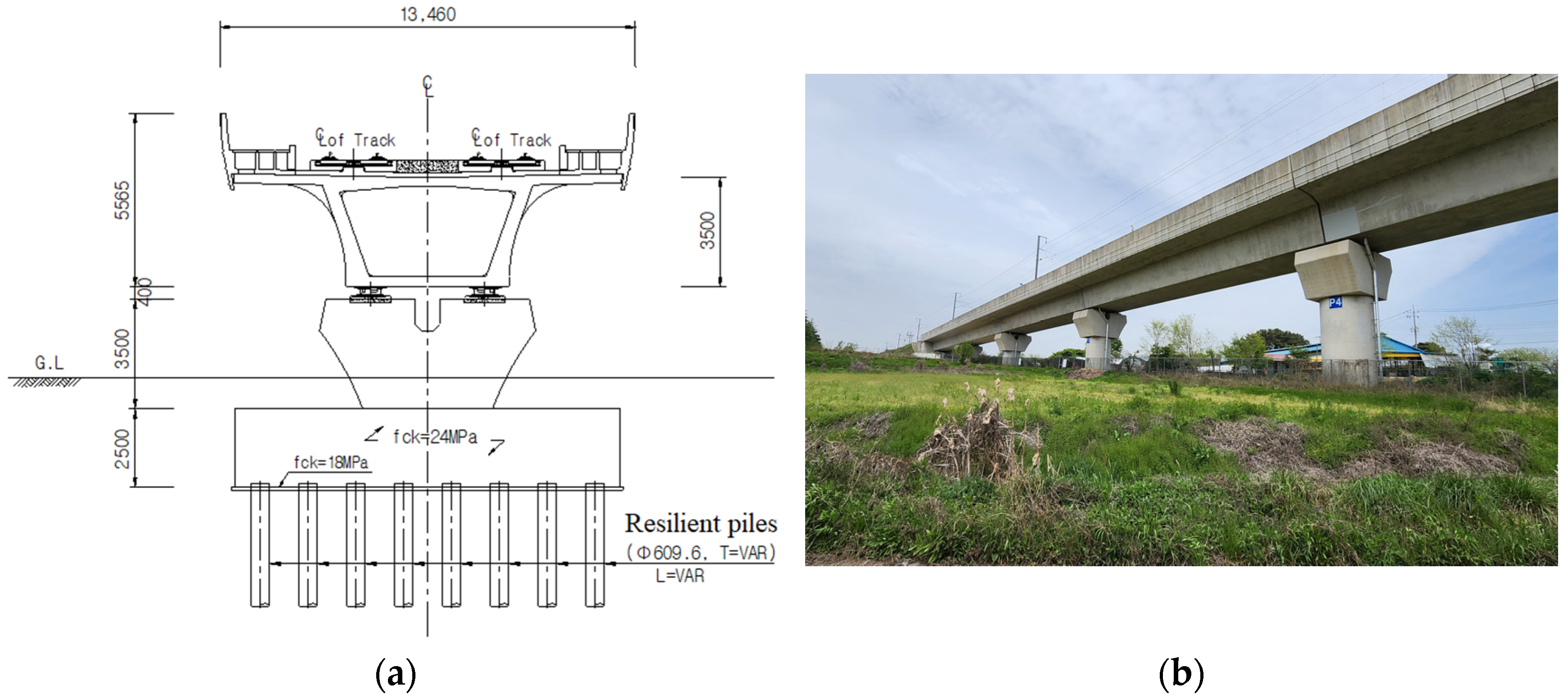
2.2. Nature of the Post-Tensioned Pre-Stressed Concrete (PSC) Box Bridge
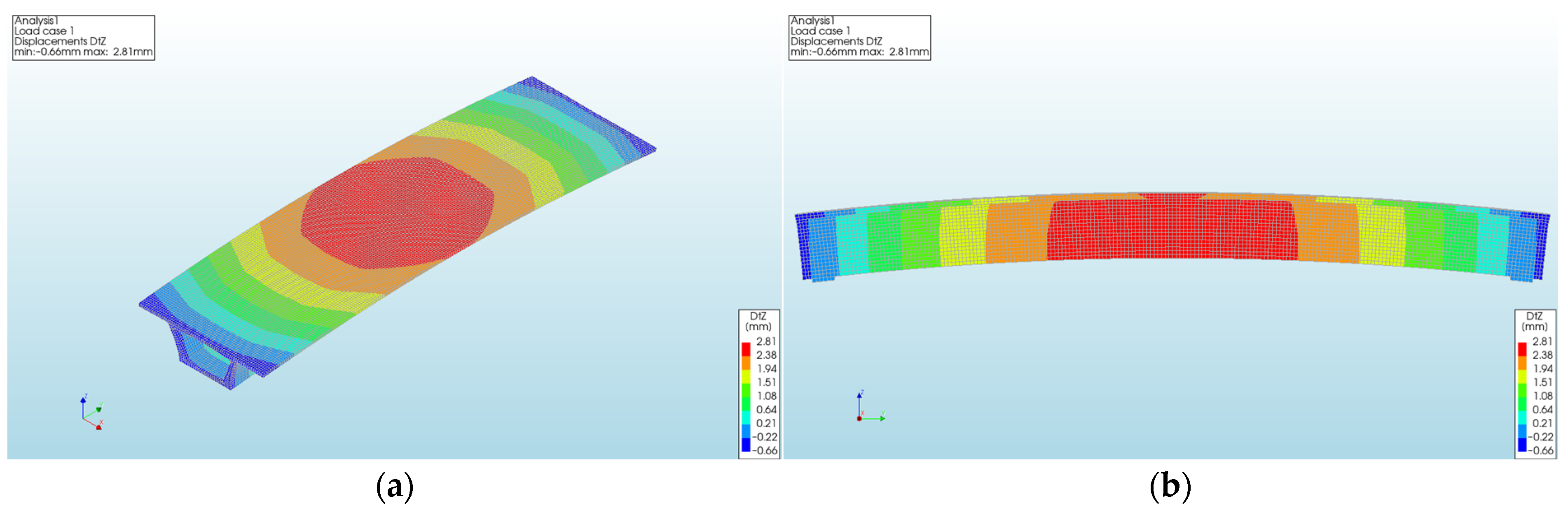
2.3. Numerical Analysis
2.4. Multi-Temporal InSAR Analysis: PS-InSAR
- A total of 30 SAR images in .slc format are imported into ENVI. Each image contains unique spatiotemporal characteristics. Because an interferogram stack is produced by combining multiple interferograms that share the same primary image, it is important to select a primary image that minimises decorrelation caused by spatial and temporal baselines during the combination stage. The programme automatically calculates the most suitable primary image. Then, a connection graph is produced, indicating the correlation between images on specific dates and the rest with the baseline length.
- Once the primary image is determined, the remaining images are aligned to the coordinate system of the primary image through co-registration. Subsequently, a flattened radar reflection intensity map is created through convolution calculation, allowing for the correction of look and squint angle errors, which occur when converting a DEM with the divergence of Earth’s curvature to the radar coordinate system.Through the interferometry process, N − 1 interferograms are generated as a result of the primary–secondary combination, which is 29, where N represents the total number of SAR images imported.
- An inversion calculation is performed to create a linear model, as expressed in Equation (4), on the flattened radar reflection intensity map. A PS candidate is selected based on the set PS threshold, with the final relative height and subsidence velocity (mm/yr) at each point at the observation end time calculated through phase unwrapping based on the surrounding reference points.
- In the linear model generated in the previous step, an additional inversion calculation is performed to remove the phase errors owing to the atmosphere, which are expressed as the constant K. The impact on the final displacement is dependent on the strength of atmospheric filter effects, and it is important to determine the appropriate spatiotemporal effect ranges of the filter. This process can result in the calculation of subsidence per filming data, and the composition of a time series. Equation (5) represents the calculation of final displacement .
- Given that the resultant displacement value is relative, the DEM file at the geocoding step is considered to convert it into actual height data. Subsequently, the analysis is finalised by the reprojection of data to the actual geographical coordinates, thus aligning the dataset with real-world locations.
3. InSAR Parameter Optimisation
3.1. Data Acquisition
3.2. Parametric Analysis
4. Results
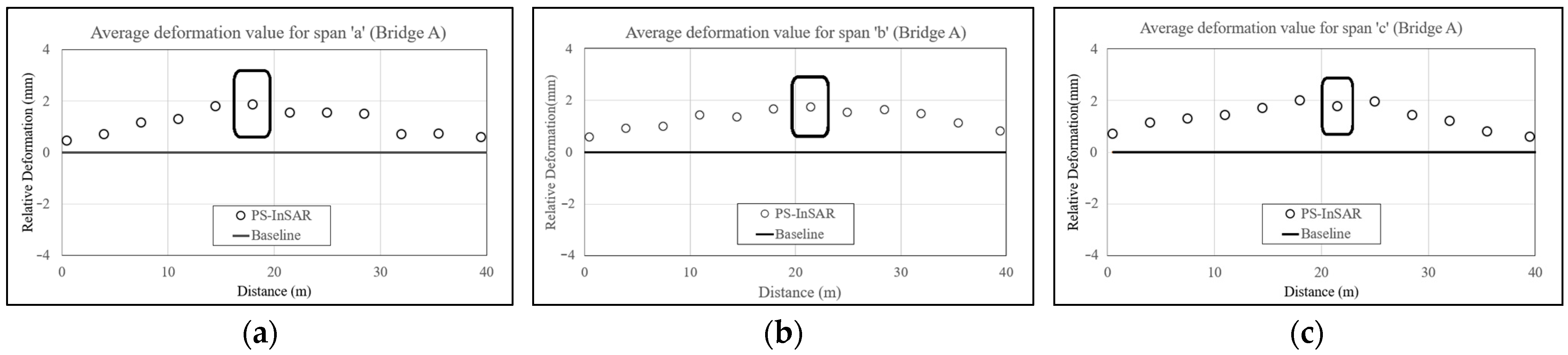
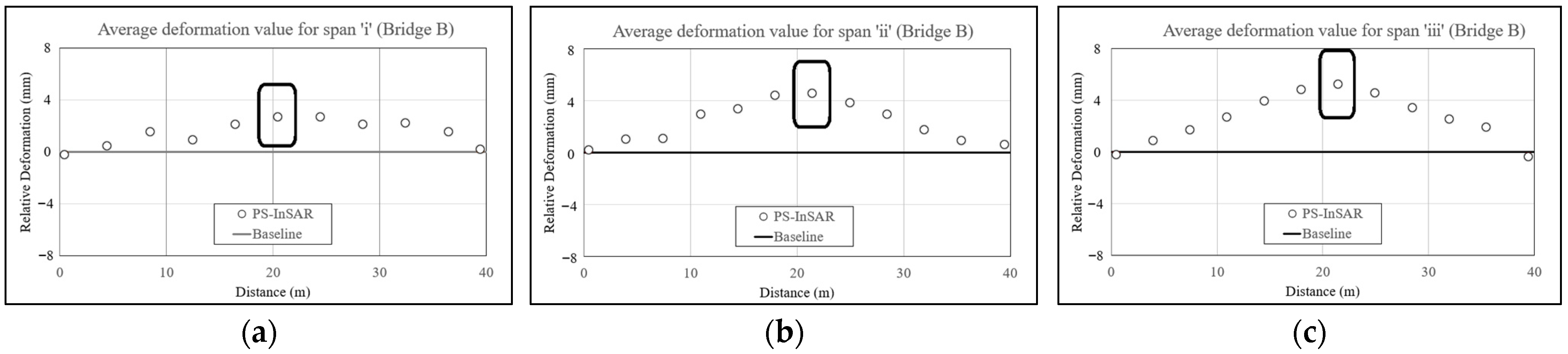
4.1. Preliminary Displacement Patterns and Observations
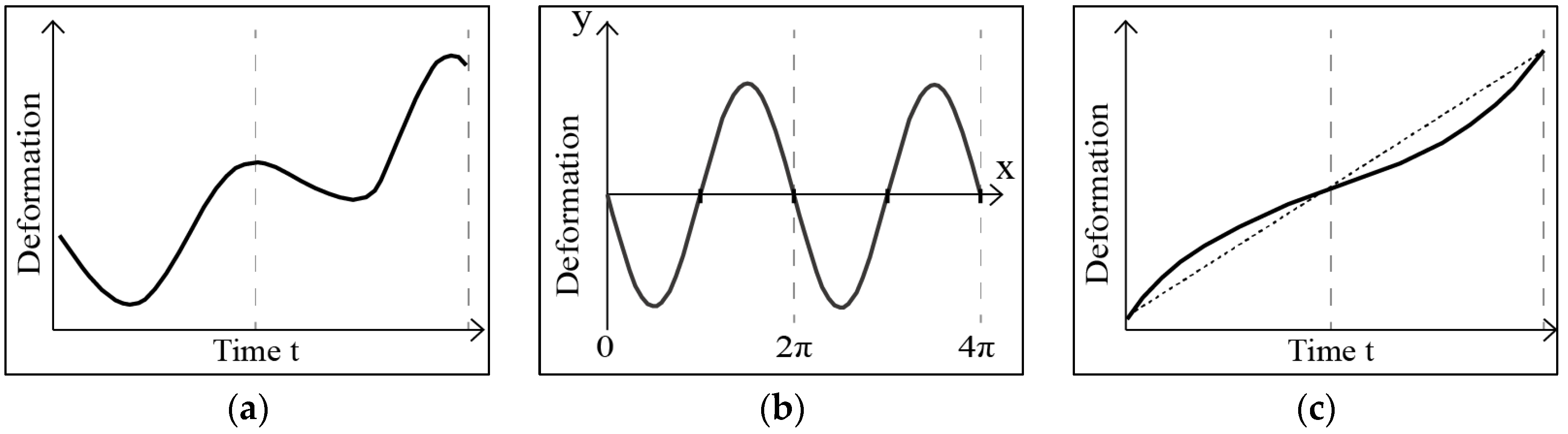
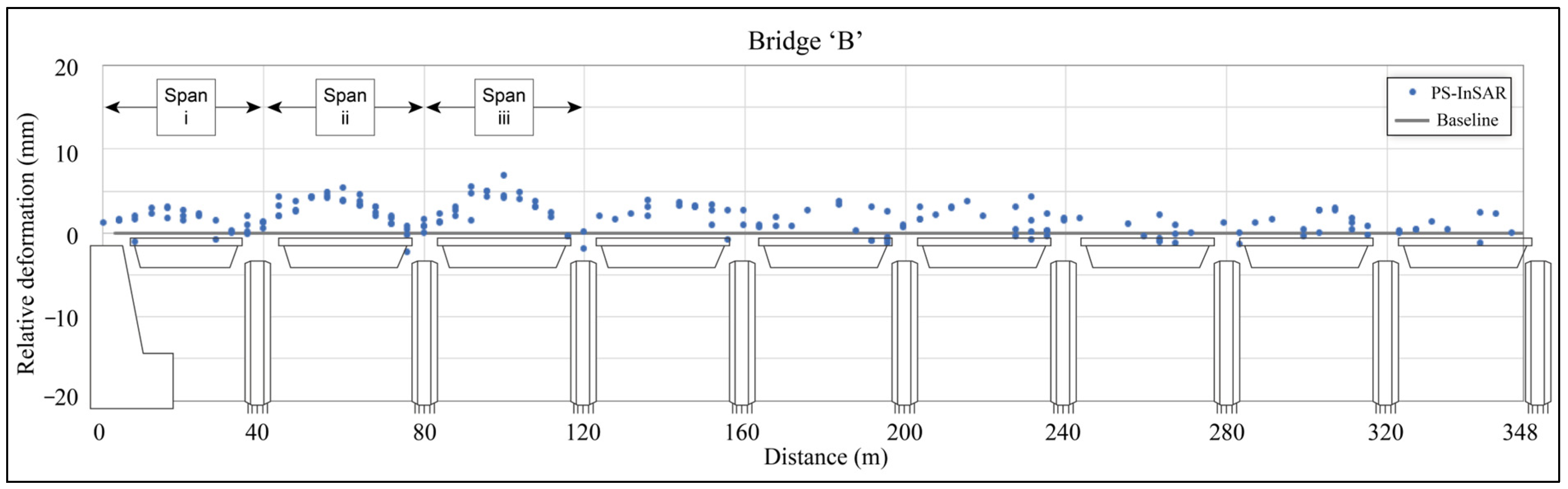
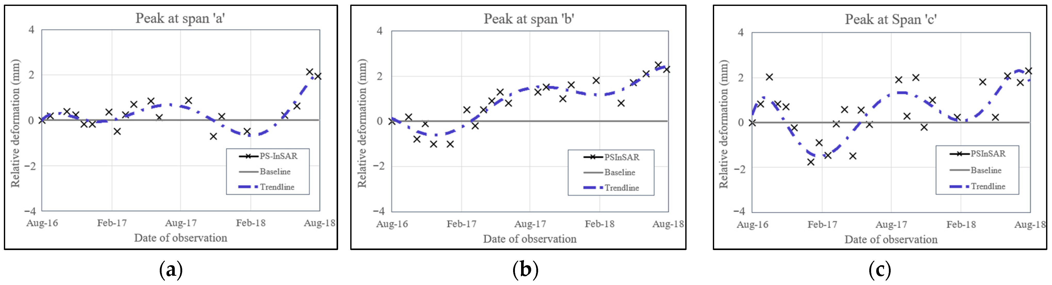
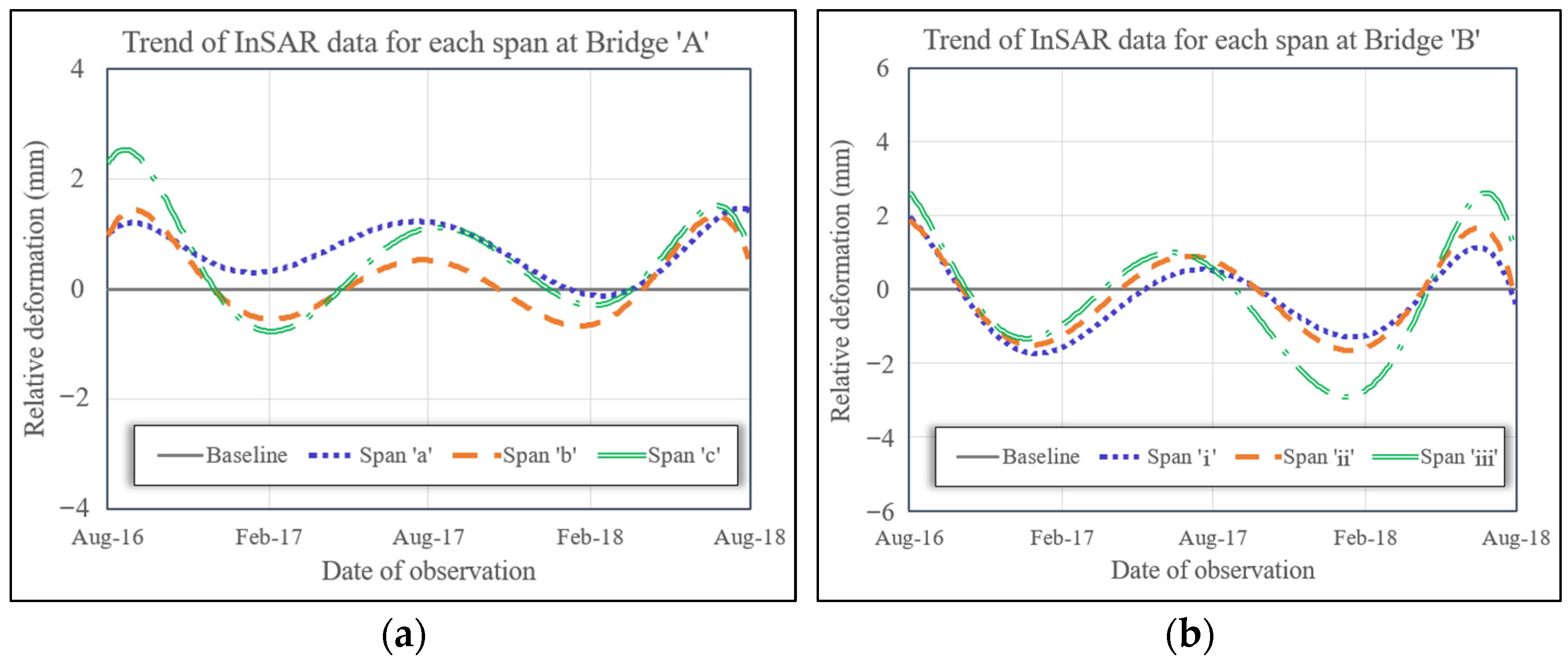
4.2. Characteristics of Long-Term Behaviour (Camber) and Results
4.3. Expansion or Contraction Owing to Temperature from Seasonal Changes
5. Conclusions
5.1. Discussion
5.2. Summary
5.3. Future Works
Author Contributions
Funding
Data Availability Statement
Conflicts of Interest
References
- Ferretti, A.; Prati, C.; Rocca, F. Nonlinear subsidence rate estimation using permanent scatterers in differential SAR interferometry. IEEE Trans. Geosci. Remote Sens. 2000, 38, 2202–2212. [Google Scholar] [CrossRef]
- Ferretti, A.; Prati, C.; Rocca, F. Permanent scatterers in SAR interferometry. IEEE Trans. Geosci. Remote Sens. 2001, 39, 8–20. [Google Scholar] [CrossRef]
- Hooper, A.; Zebker, H.; Segall, P.; Kampes, B. A new method for measuring deformation on volcanoes and other natural terrains using InSAR persistent scatterers. Geophys. Res. Lett. 2004, 31, 23. [Google Scholar] [CrossRef]
- Hooper, A. Persistent Scatterer Radar Interferometry for Crustal Deformation Studies and Modeling of Volcanic Deformation. Ph.D. Thesis, Stanford University, Stanford, CA, USA, 2006. Available online: https://web.stanford.edu/group/radar/people/Hooper_Thesis.pdf (accessed on 24 June 2024).
- Luo, Q.; Perissin, D.; Lin, H.; Zhang, Y.; Wang, W. Subsidence monitoring of Tianjin suburbs by TerraSAR-X persistent scatterers interferometry. IEEE J. Sel. Top. Appl. Earth Obs. Remote Sens. 2013, 7, 1642–1650. [Google Scholar] [CrossRef]
- Macchiarulo, V.; Milillo, P.; Blenkinsopp, C.; Giardina, G. Monitoring deformations of infrastructure networks: A fully automated GIS integration and analysis of InSAR time-series. Struct. Health Monit. 2022, 21, 1849–1878. [Google Scholar] [CrossRef]
- Macchiarulo, V.; Milillo, P.; Blenkinsopp, C.; Reale, C.; Giardina, G. Multi-Temporal InSAR for transport infrastructure monitoring: Recent trends and challenges. Proc. Inst. Civ. Eng. Bridge Eng. 2022, 176, 92–117. [Google Scholar] [CrossRef]
- Milillo, P.; Bürgmann, R.; Lundgren, P.; Salzer, J.; Perissin, D.; Fielding, E.; Biondi, F.; Milillo, G. Space geodetic monitoring of engineered structures: The ongoing destabilization of the Mosul dam, Iraq. Sci. Rep. 2016, 6, 37408. [Google Scholar] [CrossRef]
- Milillo, P.; Perissin, D.; Salzer, J.; Lundgren, P.; Lacava, G.; Milillo, G.; Serio, G. Monitoring dam structural health from space: Insights from novel InSAR techniques and multi-parametric modeling applied to the Pertusillo dam, Basilicata, Italy. Int. J. Appl. Earth Obs. Geoinf. 2016, 52, 221–229. [Google Scholar] [CrossRef]
- Delgado Blasco, J.; Foumelis, M.; Stewart, C.; Hooper, A. Measuring Urban Subsidence in the Rome Metropolitan Area (Italy) with Sentinel-1 SNAP-StaMPS Persistent Scatterer Interferometry. Remote Sens. 2019, 11, 129. [Google Scholar] [CrossRef]
- Struhár, J.; Rapant, P. Spatiotemporal visualisation of PS InSAR Generated Space–Time Series Describing Large Areal Land Deformations Using Diagram Map with Spiral Graph. Remote Sens. 2022, 14, 2184. [Google Scholar] [CrossRef]
- Chang, L.; Dollevoet, R.; Hanssen, R. Railway infrastructure monitoring using satellite radar data. Int. J. Railw. Technol. 2014, 3, 79–91. [Google Scholar] [CrossRef]
- Yang, Z. Monitoring and Predicting Railway Subsidence Using SAR and Time Series Prediction Techniques. Ph.D. Thesis, The University of Birmingham, Birmingham, UK, 2015. [Google Scholar]
- Qin, X.; Liao, M.; Zhang, L.; Yang, M. Structural health and stability assessment of high-speed railways via thermal dilation mapping with time-series InSAR Analysis. IEEE J. Sel. Top. Appl. Earth Observ. Remote Sens. 2017, 10, 2999–3010. [Google Scholar] [CrossRef]
- Milillo, P.; Giardina, G.; Perissin, D.; Milillo, G.; Coletta, A.; Terranova, C. Pre-collapse space geodetic observations of critical infrastructure: The Morandi Bridge, Genoa, Italy. Remote Sens. 2019, 11, 1403. [Google Scholar] [CrossRef]
- Jung, J.; Kim, D.; Palanisamy Vadivel, S.; Yun, S. Long-term deflection monitoring for bridges using X and C-band time-series SAR interferometry. Remote Sens. 2019, 11, 1258. [Google Scholar] [CrossRef]
- Lazecky, M.; Hlavacova, I.; Bakon, M.; Sousa, J.J.; Perissin, D.; Patricio, G. Bridge displacements monitoring using space-borne X-band SAR interferometry. IEEE J. Sel. Top. Appl. Earth Observ. Remote Sens. 2016, 10, 205–210. [Google Scholar] [CrossRef]
- Markogiannaki, O.; Xu, H.; Chen, F.; Mitoulis, S.A.; Parcharidis, I. Monitoring of a landmark bridge using SAR interferometry coupled with engineering data and forensics. Int. J. Remote Sens. 2022, 43, 95–119. [Google Scholar] [CrossRef]
- Farneti, E.; Cavalagli, N.; Costantini, M.; Trillo, F.; Minati, F.; Venanzi, I.; Ubertini, F. A method for structural monitoring of multispan bridges using satellite InSAR data with uncertainty quantification and its pre-collapse application to the Albiano-Magra Bridge in Italy. Struct. Health Monit. 2023, 22, 353–371. [Google Scholar] [CrossRef]
- Youssef, G. General Properties of Polymers; Linear elastic behavior of polymers. In Applied Mechanics of Polymers: Properties, Processing, and Behavior, 1st ed.; Elsvier: Amsterdam, The Netherlands, 2022; pp. 33–38, 79–107. [Google Scholar]
- Korean Design Standards (KDS). General Design Criteria for Railway Bridges, KDS 24 12 20. 2021. Available online: https://www.kcsc.re.kr/StandardCode/Viewer/40145 (accessed on 24 June 2024).
- Hanssen, R.F. Subsidence Monitoring Using Contigous and PS-InSAR Quality Assessment Based on Precision and Reliability. In Proceedings of the 11th FIG Symposium on Deformation Measurements, Santorini, Greece, 25–28 May 2003; Available online: https://w.fig.net/resources/proceedings/2003/2003_comm6_greece.htm (accessed on 11 August 2024).
- PS Tutorial Version 5.6.2. Available online: https://www.sarmap.ch/tutorials/PS_v562.pdf (accessed on 24 June 2024).
- Synthetic Aperture Radar and SARscape®. Available online: https://www.sarmap.ch/pdf/SAR-Guidebook.pdf (accessed on 24 June 2024).
- Berardino, P.; Fornaro, G.; Lanari, R.; Sansosti, E. A new algorithm for surface deformation monitoring based on Small Baseline differential SAR Interferometry. IEEE Trans. Geosci. Remote Sens. 2002, 40, 2375–2383. [Google Scholar] [CrossRef]
- Cusson, D.; Trischuk, K.; Hébert, D.; Hewus, G.; Gara, M.; Ghuman, P. Satellite-based InSAR Monitoring of Highway Bridges: Validation Case Study on the North Channel Bridge in Ontario, Canada. Transp. Res. Rec. 2018, 2672, 76–86. [Google Scholar] [CrossRef]
- D’Aranno, P.; Di Benedetto, A.; Fiani, M.; Marsella, M.; Moriero, I.; Baeno, J.A.P. An application of persistent scatterer interferometry (PSI) technique for infrastructure monitoring. Remote Sens. 2021, 13, 1052. [Google Scholar] [CrossRef]
- Potsis, A.; Reigber, A.; Papathanassiou, K. A phase preserving method for RF interference suppression in P-band synthetic aperture radar interferometric data. In Proceedings of the IEEE 1999 International Geoscience and Remote Sensing Symposium, Hamburg, Germany, 28 June–2 July 1999; Volume 5, pp. 2655–2657. [Google Scholar] [CrossRef]
- Reigber, A.; Ferro-Famil, L. Interference suppression in synthesized SAR images. IEEE Geosci. Remote Sens. Lett. 2005, 2, 45–49. [Google Scholar] [CrossRef]
- Giordano, P.; Turksezer, Z.; Previtali, M.; Limongelli, M. Damage detection on a historic iron bridge using satellite DInSAR data. Struct. Health Monit. 2022, 21, 2291–2311. [Google Scholar] [CrossRef]
- Demirboğa, R. Thermal conductivity and compressive strength of concrete incorporation with mineral admixtures. Build. Environ. 2007, 42, 2467–2471. [Google Scholar] [CrossRef]
- Zimmerman, R. Thermal conductivity of fluid-saturated rocks. J. Petrol. Sci. Eng. 1989, 3, 219–227. [Google Scholar] [CrossRef]


| Variables | Positions | ||||
|---|---|---|---|---|---|
| X (m) | 0 | 10 | 20 | 30 | 40 |
| DtZ (mm) 1 | −0.66 | 1.80 | 2.81 | 1.80 | −0.66 |
| Parameters | Values |
|---|---|
| Repeat Period | 11 days |
| Orbit | Descending |
| Inclination | 97.44° |
| Altitude at the equator | 514 km |
| Centre Frequency | 9.65 GHz (X band) |
| Polarisation | VV |
| Parameter Set | A | B | C |
|---|---|---|---|
| Looks [Azimuth, Range] | [2, 2] | [2, 2] | [2, 2] |
| Sub-area Overlap | 30% | 25% | 25% |
| Sub-area Merging Coherence Threshold | 0.60 | 0.66 | 0.66 |
| Mu-sigma Threshold | 70% | 60% | 60% |
| Low Pass Filter | 1200 m | 600 m | 1200 m |
| High Pass Filter | 781 days | 781 days | 365 days |
| Product Coherence Threshold | 0.65 | 0.65 | 0.65 |
| Stages | A | B |
|---|---|---|
| Interferometry Generation | Looks [Azimuth, Range] | [2, 2] |
| Interpolation Algorithm | 4th Cubic Spline Interpolation | |
| Sub-area Coverage | 25 km2 | |
| Inversion: First Step | Sub-area Overlap | 25% |
| Sub-area Merging Coherence Threshold | 0.60 | |
| SNR Threshold | 3.2 | |
| Mu-sigma Threshold | 70% | |
| Inversion: Second Step | Minimum and Maximum Displacement Velocity | −40 mm/yr (Min.) 25 mm/yr (Max.) each |
| Number of Reference Point Candidates | 5 | |
| Low Pass Filter | 1200 m | |
| High Pass Filter | 782 days | |
| Geocoding | GCP/DEM usage | SRTM 1 arc-second |
| Product Coherence Threshold | 0.65 |
| Site | Length (m) | Number of PS Point Clouds | PS Density (Counts/km2) |
|---|---|---|---|
| Bridge A | 400 | 314 | 58,321 |
| Bridge B | 348 | 311 | 65,639 |
| Sites | Total Deformation (mm) | Deformation Velocity (mm/yr) | Mean Velocity (mm/yr) | Standard Deviation σ | |
|---|---|---|---|---|---|
| Bridge | Span | ||||
| A | a | 1.25 | 0.62 | 0.91 | 0.21 |
| b | 2.01 | 1.00 | |||
| c | 2.20 | 1.10 | |||
| B | i | 6.03 | 3.01 | 3.34 | 0.25 |
| ii | 7.22 | 3.61 | |||
| iii | 6.79 | 3.39 | |||
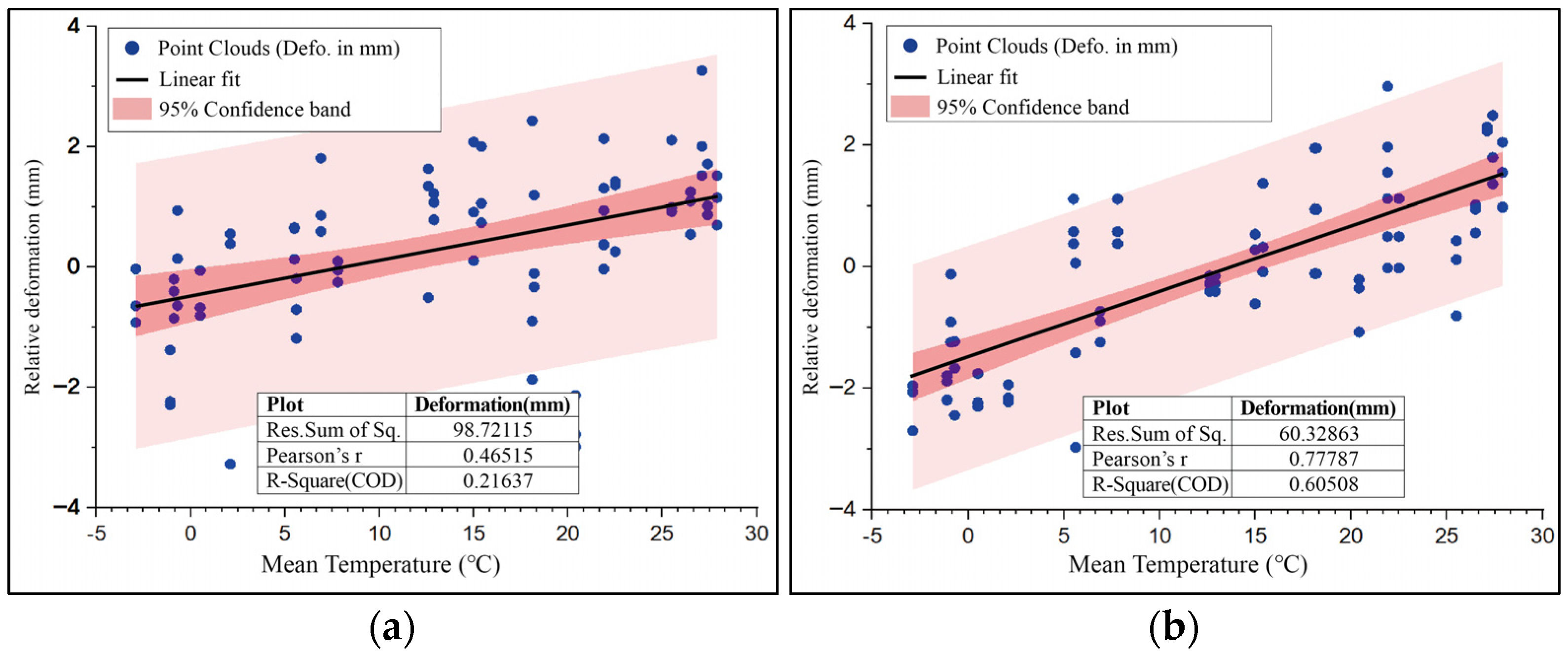
| Determination Coefficients | Bridge A | Bridge B |
|---|---|---|
| Pearson’s r | 0.465 | 0.778 |
| R2 | 0.216 | 0.605 |
| Sites | Maximum Value (mm) | Minimum Value (mm) | Range of Deformation (mm) | Expected Range of Variation at Numerical Analysis (MAX. −MIN., mm) | |
|---|---|---|---|---|---|
| Bridge | Span | ||||
| A | a | 1.20 | −0.16 | 1.36 | 2.81 |
| b | 1.35 | −0.71 | 2.06 | ||
| c | 2.39 | −0.78 | 3.17 | ||
| B | i | 1.99 | −2.01 | 4.00 | |
| ii | 1.95 | −1.92 | 3.87 | ||
| iii | 2.55 | −2.60 | 5.15 | ||
Disclaimer/Publisher’s Note: The statements, opinions and data contained in all publications are solely those of the individual author(s) and contributor(s) and not of MDPI and/or the editor(s). MDPI and/or the editor(s) disclaim responsibility for any injury to people or property resulting from any ideas, methods, instructions or products referred to in the content. |
© 2024 by the authors. Licensee MDPI, Basel, Switzerland. This article is an open access article distributed under the terms and conditions of the Creative Commons Attribution (CC BY) license (https://creativecommons.org/licenses/by/4.0/).
Share and Cite
Kim, W.; Lee, C.; Kim, B.-K.; Kim, K.; Lee, I. Leveraging Multi-Temporal InSAR Technique for Long-Term Structural Behaviour Monitoring of High-Speed Railway Bridges. Remote Sens. 2024, 16, 3153. https://doi.org/10.3390/rs16173153
Kim W, Lee C, Kim B-K, Kim K, Lee I. Leveraging Multi-Temporal InSAR Technique for Long-Term Structural Behaviour Monitoring of High-Speed Railway Bridges. Remote Sensing. 2024; 16(17):3153. https://doi.org/10.3390/rs16173153
Chicago/Turabian StyleKim, Winter, Changgil Lee, Byung-Kyu Kim, Kihyun Kim, and Ilwha Lee. 2024. "Leveraging Multi-Temporal InSAR Technique for Long-Term Structural Behaviour Monitoring of High-Speed Railway Bridges" Remote Sensing 16, no. 17: 3153. https://doi.org/10.3390/rs16173153