Comparative Study of Seafloor Topography Prediction from Gravity–Geologic Method and Analytical Algorithm

Abstract

Seafloor topography prediction can fill in sea areas without ship sounding data. However, the dependence of various topographic prediction algorithms on ship soundings varies significantly. Hence, this study explores the impact of the number and distributions of ship soundings on topographic prediction using the gravity–geologic method (GGM) and an analytical algorithm. Firstly, this study investigates the influence of ship sounding coverage on the two algorithms. The simulation results demonstrate that increasing coverage from 5.40% to 31.80%, coupled with more uniform distributions across the study area, substantially reduces the RMS error of the GGM. Specifically, the RMS error decreases from 238.68 m to 42.90 m, an improvement of 82.03%. The analytical algorithm maintains a consistent RMS error of 40.39 m because it does not depend on ship soundings. Furthermore, we select a 1° × 1° sea area (134.8°–135.8°E, 30.0°–31.0°N), and the ship soundings are divided into two control groups, Part I and Part II, with coverages of 8.19% and 33.19%, respectively. When Part II is used for calculation, the RMS error of the GGM decreases from 204.17 m to 126.95 m compared to when Part I is used, while the analytical algorithm exhibits an RMS error of 167.94 m. The findings indicate that the prediction accuracy of the GGM is significantly affected by ship soundings, whereas the analytical algorithm is more stable and independent of ship soundings. Based on simulation experiments and realistic examples, when the effective ship soundings coverage exceeds 30%, the GGM may have more advantages. Conversely, the analytical algorithm may be better. This suggests that effectively combining and utilizing different algorithms based on the ship sounding coverage can improve the accuracy of topographic prediction. This will provide a basis for integrating multiple algorithms to construct a global seafloor topography model.

1. Introduction

Ship soundings serve as the primary data source for creating detailed seafloor topography [1]. However, they are expensive, time-consuming, and challenging to collect across all global ocean regions [2]. Over the past decades, various algorithms have been developed to predict seafloor topography using gravity anomalies (mainly derived from satellite altimetry data), filling the gaps in areas where ship soundings are not available. There are several algorithms, including the gravity–geologic method (GGM) relying on Burger’s correction [3,4,5,6,7,8,9,10,11,12,13,14], and the Sandwell and Smith algorithm based on Parker’s formula [15,16,17,18,19,20]. These algorithms fundamentally depend on the strong correlation between gravity anomalies and topography and incorporate existing ship soundings to establish a linear relationship between topography and gravity anomalies. Furthermore, the vertical gravity gradient (VGG), which is the second-order derivative of the gravity potential, is more responsive to the high-frequency signals associated with the topographic relief [21,22,23,24]. Additionally, with the improvement and enrichment of satellite altimetry data, there has been a growing interest in applying VGG for topography prediction [25]. S.-S. Kim and Wessel combined gravity gradient data with a nonlinear inversion method to enhance their detection of seamounts [26]. Yang et al. effectively leveraged VGG anomalies in conjunction with simulated annealing to predict seafloor topography [27], while. Xu and Yu developed a system of analytical equations to forecast topography based on VGG anomalies [28]. Numerous global seafloor topography models have been developed using diverse algorithms [29,30,31,32], but there is a lack of comparative research on these algorithms and their integration for the construction of topography models. This is one of the initial points of this study.

Several studies comparing the GGM and Sandwell and Smith algorithms have demonstrated that the GGM is not only computationally simpler but also more efficient [33,34], which has contributed to its wider adoption. Given that the GGM is a fitting algorithm, efforts to improve it have primarily concentrated on optimizing the density constant. The optimal ‘tuning’ density difference can achieve the highest topographic prediction accuracy for the GGM [7]. Research has also explored extending the iso interval of gravity anomalies downward and identifying the optimal ‘tuning’ density difference through proportional relationships [3,4,33]. Nonetheless, these methods carry the risk of distorting the original physical meaning of density.

Relying on the Seabed-30 project, approximately 25% of the global sea area has been mapped through ship sounding data. However, it is worth noting that the remaining 75% of the sea area still requires seafloor topography prediction algorithms to bridge this gap. The effectiveness of the GGM is directly influenced by ship soundings distributions, as distributions are a prerequisite for the algorithm. How do the distributions impact the GGM? Despite its significant implications for the topographic construction of specific maritime regions, there is limited discourse on this matter. The analytical algorithm, a frontier method for predicting seafloor topography without relying on ship soundings [28,35,36,37,38], establishes a set of observational equations between topography and gravity field based on an analytical formula. This formula generates the gravity field of a single rectangular prism at any points above it [39]. Moreover, this algorithm avoids omitting higher-order terms and precisely expresses the completely analytical mathematical relationship between the gravity field and the topography. How effective are these two algorithms in filling the sea area that has not been fully covered by ship soundings data? This question serves as the starting point of this study.

Therefore, this study aims to examine the impact of ship sounding coverage on the GGM by simulating ship sounding data from various control groups. The effectiveness of the algorithm is assessed based on checking point errors and grid point errors. Grid point errors measure the portions of the sea area not covered by ship soundings, providing a means to evaluate how well the two algorithms can address the missing sea areas. Subsequently, we apply both algorithms to the actual sea area, aiming to assess their respective effectiveness. This comparative analysis serves as the foundation for integrating multiple algorithms to develop a comprehensive global seafloor topography model.

Section 1 of this paper first introduces the current research status of using gravity data to predict seafloor topography. Section 2 describes the basic principles of the GGM and analytical algorithm. Section 3 conducts numerical simulations by constructing a simulated sea area to compare the prediction accuracy of the two algorithms. Section 4 applies the two algorithms to the realistic sea area, using ship soundings as true depth values to compare the accuracy of the two algorithms. Section 5 analyzes the results of simulation experiments and realistic examples, comparing the two algorithms with different ship soundings data, and summarizes the applicable scenarios for each algorithm.

2. Theories and Methods

2.1. Gravity–Geologic Method

The GGM separates the surface-observed gravity anomaly $∆g$ into a short-wave part ${∆g}_{short}$, caused by seafloor topographic relief, and a long-wave part ${∆g}_{long}$, attributed to other effects. The linear relationship between the short-wave gravity anomalies and the topography is established by Burger’s correction formula:

$${∆g}_{short}=2\pi G\Delta \rho \left(h-H\right)$$

(1)

where $G$ represents the universal gravitational constant, $\Delta \rho$ denotes the density difference between the oceanic crust and seawater, $h$ signifies the sea depth, and $H$ represents the reference depth, which is typically chosen as either the maximum or average depth.

The key to the GGM lies in effectively differentiating the short-wave component from the observed gravity anomaly using ship soundings. Therefore, some studies extended the gravity anomaly downward to find the optimal ‘tuning’ density difference ${\Delta \rho }_{GGM}$ [7]. However, in such cases, it is common for density to lose its original physical meaning. In recent years, additional studies have utilized iterative computation [29] and integrated artificial intelligence algorithms to further enhance the accuracy of the GGM [40]. The essence of these algorithms lies in establishing an optimal correlation between ship soundings and gravity anomalies.

2.2. Analytical Algorithm

A single rectangular prism, denoted as $\mathsf{\Omega }$, has dimensions $2a$, $2b$, and $(H-h)$ for its length, width, and height, respectively. The prism is positioned on the seafloor at a maximum depth of $H$, with $h$ representing the vertical distance from the top of $\mathsf{\Omega }$ to the sea level. A coordinate system is established with the center of the bottom surface of $\mathsf{\Omega }$ as the coordinate origin. The z-axis points to the sea level. The points of integration within $\mathsf{\Omega }$ are denoted by $(\xi ,\psi ,\zeta )$. Consequently, the gravity $g\left(P\right)$ generated by $\mathsf{\Omega }$ at any point $P(x,y,z)$ on the sea level can be expressed as [36,39,41]:

$$g\left(P\right)={\left.{\left.{\left.G\rho \left[\xi \mathit{ln}\left(\psi +r\right)+\psi \mathit{ln}\left(\xi +r\right)-\zeta \cdot \mathit{arctan}{\displaystyle \frac{\xi \psi }{\zeta r}}\right]\right|}_{x-a}^{x+a}\right|}_{y-b}^{y+b}\right|}_H^h$$

(2)

where $r=\sqrt{{\left(x-\xi \right)}^2+{\left(y-\psi \right)}^2+{\left(z-\zeta \right)}^2}$, $G$ is the universal gravitational constant, and $\rho$ is the density of $\mathsf{\Omega }$.

In fact, the seafloor topography can be divided into several rectangular regions. If we ensure that the rectangles have equal length and width, we can accurately capture the undulations of the seabed topography by determining the height of each rectangle. By replacing the density $\rho$ in Equation (2) with $\Delta \rho$, which represents the difference in density between oceanic crust and seawater, we can derive the gravity anomaly instead of gravity. This gravity anomaly is generated by the undulation of seafloor topography. Similarly, by utilizing Equation (2), an array of observational equations can be formulated to calculate the depth $h$ when the gravity anomaly is known. The detailed structure of the system of equations and the algorithmic solution procedure can be found in [28,36,37].

3. Simulation Experiments

3.1. Simulated Data

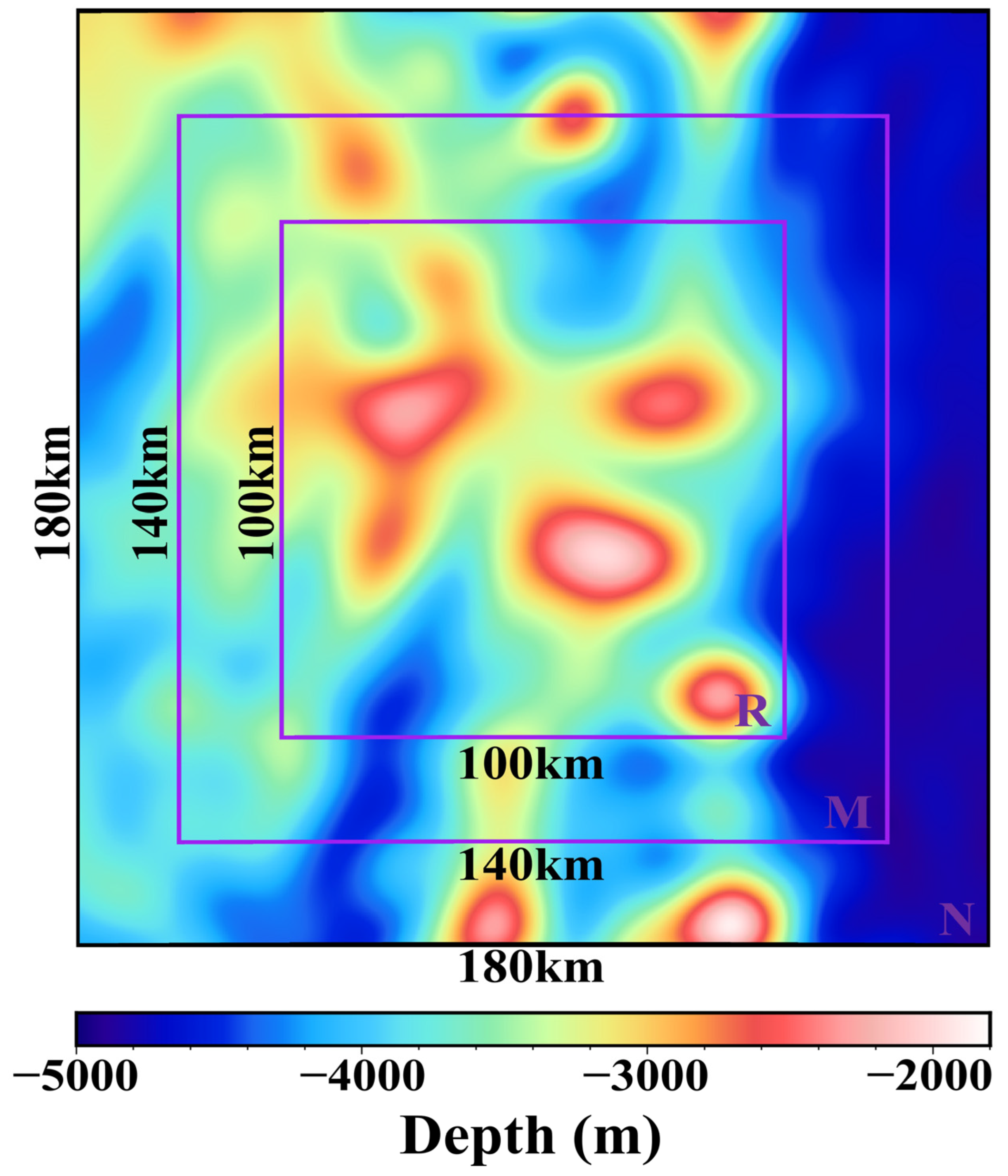
3.1.1. Simulated Seafloor Topography and Gravity Anomaly

In this section, we simulate a sea area with known true topography (error-free depths) using numerical simulation methods. This sea area has a resolution of 2 km, a size of 180 km × 180 km, and contains 90 × 90 grid points, as shown in Figure 1. The study area R measures 100 km × 100 km, containing 50 × 50 grid points. The maximum depth is recorded at −4601.39 m, while the minimum depth is −2001.32 m. The average depth is approximately −3427.55 m. The influence of topographic relief still persists beyond the study area. To address this, the boundary area M and the far area N are defined by extending 40 km outward from the boundary of R twice. The influence of the farther sea area still exists, but it is a low-frequency small quantity. Furthermore, the irregular distributions of mass within the Earth’s inner layer also exert some influence. However, the GGM does not account for this particular impact. Additionally, the effect of this deviation on the analytical algorithm is relatively minor compared to the boundary and far areas. Therefore, this study does not delve into a detailed discussion of this aspect.

Setting the density difference $\Delta \rho$ as 1.6 g/cm³, the gravity anomalies generated by R, M, and N in the study area R are forward modeled using Equation (2), as shown in Figure 2 (denoted by $\Delta g_R$, $\Delta g_M$, and $\Delta g_N$, respectively). Specifically, Figure 2a depicts the spatial distributions of $\Delta g_R$.

We calculate $\Delta g_R$, $\Delta g_M$, and $\Delta g_N$, as shown in

Table 1. Simulated gravity anomalies in the study area R.

Area	Max (mGal)	Min (mGal)	Avg (mGal)	Range (mGal)	SD (mGal)
Study Area R	234.22	13.66	108.29	220.56	46.88
Boundary Area M	108.07	2.67	14.82	105.4	16.10
Far Area N	8.84	1.27	2.65	7.57	1.24

Note: Max denotes the maximum value of the gravity anomalies in a specific area; Min denotes the minimum value; Avg denotes the average value; Range denotes the difference between the maximum and minimum values; SD denotes the standard deviation.

. The maximum values of $\Delta g_M$ and $\Delta g_N$ decrease to 46.14% and 3.77% of $\Delta g_R$, respectively. Furthermore, their standard deviations decrease to 34.34% and 2.65%, respectively. In other words, $\Delta g_M$ exhibits high-frequency distributions while $\Delta g_N$ shows low-frequency distributions. (Here, we define the confidence interval of 95% as the upper limit. If a value decreases to 5% or less of the maximum value, it is regarded as low-frequency). To address both high-frequency and low-frequency error disturbances, we employ specific algorithms to attenuate each of them. For high-frequency errors, we utilize regularization techniques, while for low-frequency errors, we incorporate error terms to mitigate their impact [28,35].

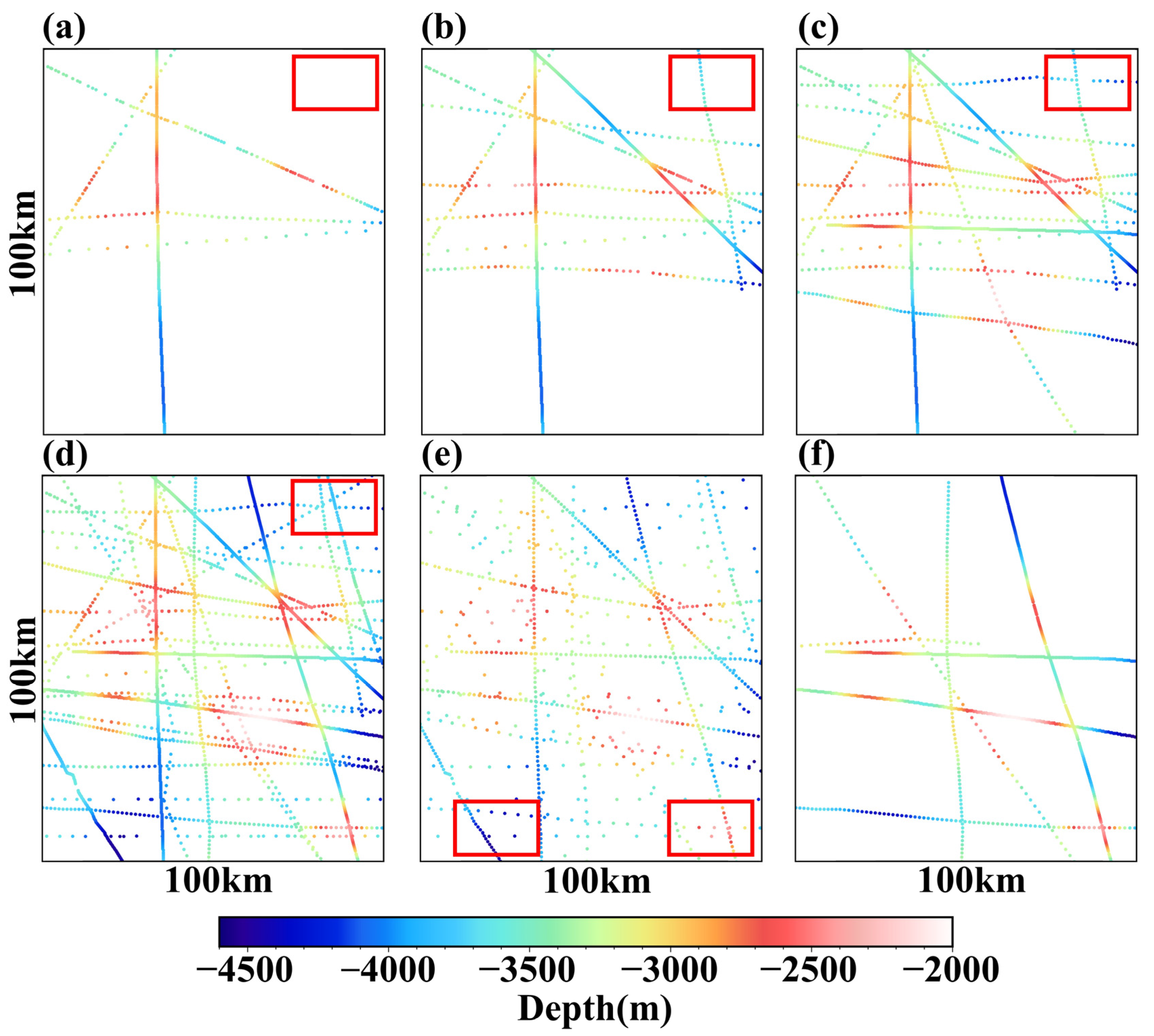
3.1.2. Simulated Ship Soundings

The GGM is significantly influenced by both the number and spatial distributions of ship soundings, while the analytical algorithm does not rely on them, as demonstrated by the simulation experiments conducted in Section 3.3. Therefore, we simulate six sets of ship soundings and illustrate their spatial distributions in Figure 3. The depth value at each ship sounding point represents the true depth of the simulated sea area. The number of ship soundings progressively increases from Group 1 to Group 4 along the survey lines, whereas Group 5 and Group 6 have an equal number of ship soundings but different distributions.

The statistical analysis of the ship soundings is shown in

Table 2. Simulated ship soundings.

Groups	Number	Coverage	Max (m)	Min (m)	Avg (m)
Group 1	434	5.4%	−2471.3	−4103.39	−3299.1
Group 2	858	10.76%	−2304.39	−4401.61	−3338.99
Group 3	1331	17.68%	−4585.58	−2134.43	−3309.82
Group 4	2614	31.80%	−4585.95	−2050.43	−3357.43
Group 5	872	16.12%	−4585.58	−2057.5	3356.58
Group 6	872	10.88%	−4525.84	−2050.43	−3298.86

Note: Coverage denotes the ratio of grid points with ship soundings to total grid points.

. From Group 1 to Group 4, the number of sounding points gradually increased from 434 to 2614. Similarly, the coverage grew from 5.44% to 31.80%, where coverage represents the ratio of grids with depth data to the total grids. Concurrently, the distributions of these points became more uniform across the entire study area. Group 5 (Figure 3e) are acquired from Group 4 (Figure 3d) by reducing the sampling rate, leading to reduced uniformity. These modifications result in a significant decrease of 66.7% in the number of sounding points and a corresponding reduction in coverage by 49.3%. Group 5 and Group 6 (Figure 3f) have the same number of sounding points, but their spatial distributions exhibit a notable disparity. Specifically, their respective coverage percentages diverge significantly, with Group 5 accounting for 16.12% and Group 6 occupying a lesser extent of 10.88%.

3.2. Impact of Ship Soundings on the GGM

We incorporate a random error of 3 mGal into the gravity anomaly $∆g$ ($\Delta g=\Delta g_R$ + $\Delta g_M$ + $\Delta g_N$) in the designated study area R. Since the GGM requires known ship soundings as input to predict the seafloor topography, in each group of ship soundings, we uniformly select 50% of the points for calculations, while the remaining 50% serve as checking points. The calculating points are used as input for the GGM, and the checking points are used to assess the error between the predicted topography and the true topography. It is worth noting that because of the uniform selection, the calculating points and checking points still have the same spatial distribution as the original ship soundings. The prediction results and error distributions on 50 × 50 grid points for each group are shown in Figure 4. We assess overall performance by computing the root mean square (RMS) errors for both the checking points and grid points. The checking points do not participate in the calculation, and they exhibit minimal errors since they are situated close to the calculating points. Conversely, the grid points refer to points that remain uncovered by ship soundings, representing blank areas of the sea. They are usually located far from the calculating points. The errors at these points serve as a valuable measure to assess the effectiveness of the prediction algorithms.

Figure 4a–d depicts the topographic outcomes obtained from the GGM for Group 1 through Group 4, respectively. Correspondingly, Figure 4h–k illustrates the error distributions of the prediction results relative to the simulated topography. From the topography results, it is evident that the overall shape of each group of topography remains consistent. Because the GGM is a fitting algorithm, the inverted topography and gravity anomaly also have strong similarity. With the increasing availability of ship soundings, the maximum and minimum value of the topography prediction results gradually converge towards the true values. In other words, the accuracy of the prediction results heavily depends on the presence or absence of ship sounding coverage. This conclusion is further supported by the error distributions of the prediction’s results. It is evident from the red boxes positioned in the upper right corner of Figure 3a–d that there is a gradual increase in ship soundings from Group 1 to Group 4. This increase correlates with the reduction in errors illustrated in the upper right corner of Figure 4h–k.

According to Table 2, comparing Group 5 and Group 6, we observe that both groups have the same number of sounding points. However, the coverage of Group 5 is 16.1%, compared to 10.8% for Group 6. Upon analyzing the RMS errors of the prediction results (as shown in

Table 3. RMS error of the two algorithms (3 mGal random error).

Groups	RMSGGM (m)		RMSAA (m)		${\mathbf{\Delta }\mathit{\rho }}_{\mathit{G}\mathit{G}\mathit{M}}$ (g/cm3)
	Checking Points	Grid Points	Checking Points	Grid Points
Group 1	14.17	238.68	33.90	40.39	3.30
Group 2	13.66	158.07	31.52	40.39	3.00
Group 3	13.08	126.01	31.15	40.39	3.40
Group 4	15.03	42.90	32.09	40.39	2.60
Group 5	30.51	52.60	31.77	40.39	1.80
Group 6	8.89	142.88	30.99	40.39	3.50

Note: AA denotes the analytical algorithm.

), it is apparent that the checking point and grid point errors improve as the coverage increases. Specifically, the RMS errors for checking points and grid points improve by 21.4% and 35.5%, respectively. This demonstrates that the ship soundings coverage significantly influences accuracy of prediction result. Additionally, when comparing Group 3 and Group 5, we observe that the coverage in both groups is similar. However, there is a notable difference in the RMS errors of the results at the checking points: 13.08 m for Group 3 and 30.51 m for Group 5. Interestingly, this pattern is reversed for the RMS errors at the grid points, where Group 3 shows an RMS error of 126.01 m and Group 5 shows an RMS error of 52.6 m. This may appear contradictory at first glance. However, upon comparing the distributions of the ship soundings in Group 3 (Figure 3c) and Group 5 (Figure 3e), we find that the distribution of sounding points in Group 3 is more centralized, leading to a concentration of sounding points used in calculation and checking points. The similarity among the ship soundings leads to a lower RMS error at checking points. The distribution of the sounding points in Group 5 is more decentralized, covering more special sea area (area with large topographic undulations and dramatic changes in gravity anomalies), as shown by the red box area in Figure 3e. This leads to higher accuracy in the prediction results of Group 5 at the grid points. This reveals the issue of coverage efficiency: with the same coverage, better coverage of special sea areas leads to higher accuracy in prediction results.

3.3. Stability of Two Algorithms

In Section 3.2, we analyzed the dependency of the GGM on ship sounding data. In this section, we further discuss the stability of the GGM and the analytical algorithm using simulation methods, including the impact of ship sounding coverage and gravity anomaly errors on both algorithms.

The topographic results and error distribution of the analytical algorithm are shown in Figure 4g,n. Ship soundings are not required for the algorithm. Instead, it effectively utilizes the observed gravity anomalies presented in Section 3.1.1. The prediction errors are primarily influenced by three factors: the boundary area M, the far area N, and random errors. Table 3 presents statistical results of the RMS errors, showing that the analytical algorithm exhibits stable RMS errors at the checking and grid points, which are approximately 30 m and 40 m, respectively. Additionally, based on the RMS errors of the grid points, it can be concluded that the analytic algorithm exhibits superior accuracy compared to the GGM. This implies that the prediction results achieved by the analytical algorithm yield more accurate topography in sea areas not covered by ship soundings. However, the GGM demonstrates greater advantages in sea areas with effective coverage (The effective coverage indicates that the ship soundings are evenly distributed throughout the study area, especially in the area with large topographic relief), as it effectively incorporates the ship sounding data.

Based on the analysis of the above results, it is recommended to utilize diverse algorithms to enhance the accuracy of the seafloor topographic model in different sea areas, depending on the extent of ship sounding coverage. In areas covered well by ship soundings, the GGM proves advantageous. Conversely, in regions with limited coverage, the analytical algorithm has higher prediction accuracy. Based on the simulation results, it can be observed that the prediction accuracy of the GGM is close to that of the analytical algorithm when the effective coverage reaches 31.80%. Additionally, it also shows the stability of prediction accuracy of the analytical algorithm without depending on ship soundings. Based on the evaluation results from the Seabed-30 program, as of 2023, the average ship sounding coverage in global sea areas is only about 25%, with less than 30% in most sea areas. This indicates that the incorporation of various algorithms based on ship sounding coverage in building the global seafloor topography model could effectively improve the accuracy.

According to the measured density data of the CRUST 1.0 [42], the density of oceanic crust is generally between 2.6–2.9 g/cm³, while the density of seawater is about 1.03 g/cm³. Therefore, the density difference in the GGM should theoretically be between 1.57–1.87 g/cm³. In the simulation experiment, this value is 1.6 g/cm³. However, the optimal density difference in the GGM, as shown in the last column of Table 3, indicates that the ${\Delta \rho }_{GGM}$ of the remaining groups no longer retains its original physical significance except that Group 5 is 1.8 g/cm³, which is closer to the theoretical value. In contrast, the analytical algorithm always sets the density difference to 1.6 g/cm³, maintaining its physical significance.

Furthermore, we analyze the error resistance properties of the two algorithms. To evaluate their performance, we introduce random errors ranging from 1 to 5 mGal into Group 1 to Group 4. The anti-error ability of the algorithms is shown in Figure 5, considering different distributions of ship soundings. In Figure 5, the horizontal axis represents the random errors added to the gravity field of the simulated sea area, and the vertical axis represents the RMS error between the seafloor topography prediction results by the GGM or analytical algorithm and the true topography. Since the GGM requires known ship sounding data as input to predict the topography, using different sets of ship soundings will result in different RMS curves. However, due to the independence of the analytical algorithm from ship soundings, it results in just a single RMS curve. As discussed in the previous section, the RMS error of the GGM at the checking points is smaller. This is primarily due to their extraction from the vicinity of the sounding points used for calculation in the GGM. As the ship soundings coverage expands, the GGM demonstrates an improved capability to withstand random errors, as evident from the RMS errors of both algorithms at the grid points. Specifically, as the coverage increases from 5.4% to 31.8%, the random error remains at 5 mGal while the RMS error of the prediction results at the grid points decreases significantly from 385.5 m to 57.4 m. In other words, the coverage expands by a factor of 4.9, leading to a corresponding increase in the accuracy of the prediction results by a factor of 5.7. When comparing the GGM and the analytical algorithm, it can be observed that, for Group 1 to Group 3, the analytical algorithm outperforms the GGM in its ability to withstand random errors. Until Group 4, specifically when the ship soundings coverage reaches 31.8%, the GGM demonstrates an error-resistant property comparable to that of the analytical algorithm. In other words, the stability of the GGM is heavily dependent on ship soundings. The analytical algorithm demonstrates more significant stability in the presence of random errors. When the gravity anomaly includes a random error within 5 mGal, the RMS error of the analytical algorithm at the grid points is always less than 70 m.

4. Realistic Examples

4.1. Gravity Anomaly and Ship Soundings

We used numerical simulations to compare the disparities between the two algorithms in Section 3. In this Section we chose a 1° × 1° sea area (134.8°–135.8°E, 30.0°–31.0°N) to accurately predict the seafloor topography, thus validating the efficacy of the two algorithms. The gravity anomaly model (EIGEN-6C4) used for prediction is obtained from the German Research Center for Geosciences (GFZ, http://icgem.gfz-potsdam.de, accessed on 1 December 2023) as depicted in Figure 6a. Its maximum value, minimum value, and standard deviation are 36.47 mGal, 7.16 mGal, and 4.83 mGal, respectively. The ship soundings, sourced from the National Oceanic and Atmospheric Administration (NOAA, https://www.ncei.noaa.gov, accessed on 1 December 2023), include a total of 2446 sounding points in the selected sea area, as shown in Figure 6b. These sounding points range from a minimum of −5080 m to a maximum of −3250 m. After gridding, the ship soundings account for a total of 1398 points, while the total number of grid points is 60 × 60. This means that 61.17% of the sea area is still not covered by the ship soundings. It is worth noting that the RMS error of EIGEN-6C4 is around 3–5 mGal globally, while 95% of ship sounding points are accurate to within 0.47% of the depth [43]. Considering that ship soundings have the highest accuracy among all current depth measurement methods, we use them as the true values for calculating and checking. Furthermore, by comparing the gravity anomaly model with the distributions of ship soundings, it is evident that the depth fluctuations indicated by the ship soundings can effectively mirror the changing characteristics of the gravity anomaly. That is, there are sounding points in the area with large fluctuations of gravity anomaly, and the two have strong similarity. It can be inferred from the simulation results in Section 3 that the distributions of ship soundings in the selected sea area significantly benefit the performance of the GGM. Additionally, Figure 6c also shows the topography of the selected area from the ETOPO-1 model provided by GFZ, containing 60 × 60 grid points, to enhance the impression of the topographic undulations in this area.

Similar to the control group in the simulation experiment, we divide the ship soundings into two parts. The first part of the ship soundings (Part I) consists of 5 survey lines with 820 points, selected in a more centralized distributions, as shown in Figure 7a, resulting in a coverage of 8.19%. The second part of the ship soundings (Part II) consists of 1626 points, as shown in Figure 7b, uniformly distributed throughout the entire selected sea area, resulting in a coverage of 33.47%. In this way, we create a control group in which Part I is used for calculation and checking, like the ship soundings in the simulation experiment, and Part II is only used for checking, like the grid points in the simulation experiment. Conversely, Part II is used for calculation and checking while Part I is only used for checking. The statistical results for the sounding points of the two parts are shown in

Table 4. Statistics for sounding points in the selected area.

Depths	Number	Coverage	Max (m)	Min (m)	Avg (m)
Part I	820	8.19%	−4761	−3946	−4391.19
Part II	1626	33.19%	−5080	−3250	−4393.34
All	2446	38.53%	−5080	−3250	−4392.62

.

When either Part I and Part II is used for the GGM, we uniformly extract two-thirds of this part for calculation, and the remaining points are used as checking points, while the other part that is not used for the GGM is entirely used for checking points. This approach resulted in the GGM generating two prediction seafloor topography models, based on the calculations using Part I or Part II. The analytical algorithm, however, operates independently of the ship soundings and generates a single model. Since the GGM requires the selection of an optimal density difference, Figure 8 illustrates the “tuning” density difference curves associated with the prediction using Part I and Part II. As shown in Figure 8, when Part I and Part II are used for the GGM, the optimal “tuning” density differences are 0.4 g/cm³ and 1.0 g/cm³, respectively. The density difference of the analytical algorithm is always 1.6 g/cm³.

4.2. Analysis of Realistic Case Results

Figure 9a,b shows the topographic results on 60 × 60 grid points obtained by the GGM when Part I and Part II are used for calculation. The maximum values are −5103.74 m and −4805.82 m, respectively, indicating a difference of approximately 300 m. The minimum values exhibit a disparity of approximately 600 m. As shown in

Table 5. RMS errors at the checking points of the GGM and the analytical algorithm.

Algorithms	RMSPart I (m)	RMSPart II (m)
GGMPart I	29.83	204.17
GGMPart II	91.81	126.95
Analytical Algorithm	115.79	167.94

Note: RMS_{Part I/II} denotes the RMS errors at the checking points of Part I/II; GGM_{Part I/II} denotes GGM using Part I/II for calculation.

, the checking points of Part I exhibit RMS errors of 29.83 m and 91.81 m, respectively, while the checking points of Part II demonstrate RMS errors of 204.17 m and 126.95 m, respectively. These results align with the simulation findings, indicating that as the ship sounding coverage increases, the prediction accuracy at the grid points improves. Additionally, Part I is more concentrated, resulting in relatively smaller errors at the checking points of Part I when the two-thirds of this part were used for the GGM.

The topographic results on 60 × 60 grid points of the analytical algorithm are shown in Figure 9c. The maximum and minimum values are −4617.14 m and −4100.06 m, respectively, and the average value is −4385.39 m. The RMS errors at the checking points of Part I and Part II are 115.79 m and 167.94 m, respectively. The RMS error at the checking points of Part II is better than the 204.17 m from the GGM when Part I is used for calculation, and worse than the 126.95 m from the GGM when Part II is used for calculation. This aligns with the results of the simulation experiment, where, when the ship soundings coverage is small, the analytical algorithm exhibits superior prediction accuracy in the blank sea area. As coverage expands, the GGM gradually demonstrates its advantages.

Furthermore, we analyze the error distributions at checking points of Part II, as shown in Figure 9d,f. As depicted in Figure 9d, larger errors are observed when Part I is used for the GGM. This discrepancy primarily arises from the inadequate coverage of the selected sea area by the ship soundings of Part I used in the calculation. The maximum error of the analytical algorithm is −598.37 m, occurring at the location marked by the red box in Figure 9f. Notably, this occurs in the most obvious area of topographic relief in Figure 9c. We applied an error threshold of 5% (95% confidence interval) derived from the mean value of the ship soundings. Consequently, the permissible absolute error is 219.63 m (5% of 4392.62 m). In reviewing the error distributions of the GGM using Part I and Part II for calculation, as well as the analytical algorithm, we observe that the percentages of absolute errors within 219.63 m are 77.86%, 92.99%, and 84.13%, respectively. This suggests that more than 80% of the prediction results from the GGM using Part II for calculation and the analytical algorithm successfully meet the required accuracy threshold.

5. Conclusions

By integrating the findings from simulation experiments and realistic examples, this study can be summarized as follows: (1) The GGM requires known ship soundings as input to predict topography, while the analytical algorithm does not; (2) Simulation experiments indicate that in sea areas where the coverage of ship soundings is less than 30%, the analytical algorithm provides more accurate topography predictions than the GGM. However, as the coverage gradually increases and exceeds 30%, the accuracy of the GGM improves and surpasses that of the analytical algorithm. It is worth noting that this coverage must be effective, meaning that the ship soundings are evenly distributed across the entire study area, especially in regions with significant topographic variation; (3) the GGM tends to lose the original physical meaning of the density difference. In contrast, the analytic algorithm preserves the physical significance. This advantage can be utilized in forward calculation to effectively separate gravity anomalies generated by topographic relief and other factors; (4) The realistic example results indicate that the RMS error of the analytical algorithm at the checking points of Part II is 167.94 m. In comparison, the RMS errors of the GGM using Part I and Part II for calculation are 204.17 m and 126.95 m, respectively. The RMS error result of the analytical algorithm falls between the two RMS errors of the GGM. It is worth noting that the corresponding coverage of Part I and Part II are 8.19% and 33.47%, respectively. This conclusion is in line with the findings from the simulation experiments. It suggests that, during the realistic prediction process, selecting the appropriate algorithms based on the coverage can effectively improve the accuracy of topography in uncharted sea areas. In the future, our aim is to integrate multiple algorithms to construct a comprehensive global seafloor topography model.

References

1. Weatherall, P.; Marks, K.M.; Jakobsson, M.; Schmitt, T.; Tani, S.; Arndt, J.E.; Rovere, M.; Chayes, D.; Ferrini, V.; Wigley, R. A New Digital Bathymetric Model of the World’s Oceans. Earth Space Sci. 2015, 2, 331–345. [Google Scholar] [CrossRef]
2. Sandwell, D.T.; Smith, W.H.F.; Gille, S.; Kappel, E.; Jayne, S.; Soofi, K.; Coakley, B.; Géli, L. Bathymetry from Space: Rationale and Requirements for a New, High-Resolution Altimetric Mission. Comptes Rendus. Géosci. 2006, 338, 1049–1062. [Google Scholar] [CrossRef]
3. Hsiao, Y.-S.; Kim, J.W.; Kim, K.B.; Lee, B.Y.; Hwang, C. Bathymetry Estimation Using the Gravity–Geologic Method: An Investigation of Density Contrast Predicted by the Downward Continuation Method. Terr. Atmos. Ocean. Sci. 2011, 22, 347. [Google Scholar] [CrossRef]
4. Hsiao, Y.-S.; Hwang, C.; Cheng, Y.-S.; Chen, L.-C.; Hsu, H.-J.; Tsai, J.-H.; Liu, C.-L.; Wang, C.-C.; Liu, Y.-C.; Kao, Y.-C. High-Resolution Depth and Coastline over Major Atolls of South China Sea from Satellite Altimetry and Imagery. Remote Sens. Environ. 2016, 176, 69–83. [Google Scholar] [CrossRef]
5. Hwang, C. A Bathymetric Model for the South China Sea from Satellite Altimetry and Depth Data. Mar. Geod. 1999, 22, 37–51. [Google Scholar] [CrossRef]
6. Ibrahim, A.; Hinze, W.J. Mapping Buried Bedrock Topography with Gravity. Groundwater 1972, 10, 18–23. [Google Scholar] [CrossRef]
7. Kim, J.W.; Von Frese, R.R.B.; Lee, B.Y.; Roman, D.R.; Doh, S.-J. Altimetry-Derived Gravity Predictions of Bathymetry by the Gravity-Geologic Method. Pure Appl. Geophys. 2011, 168, 815–826. [Google Scholar] [CrossRef]
8. Kim, K.B.; Yun, H.S. Satellite-Derived Bathymetry Prediction in Shallow Waters Using the Gravity-Geologic Method: A Case Study in the West Sea of Korea. KSCE J. Civ. Eng. 2018, 22, 2560–2568. [Google Scholar] [CrossRef]
9. Ouyang, M.-D.; Sun, Z.-M.; Zhai, Z.-H. Predicting bathymetry in South China Sea using the gravity–geologic method. Chin. J. Geophys. 2014, 57, 2756–2765. [Google Scholar]
10. Wan, X.; Han, W.; Ran, J.; Ma, W.; Annan, R.F.; Li, B. Seafloor Density Contrast Derived From Gravity and Shipborne Depth Observations: A Case Study in a Local Area of Atlantic Ocean. Front. Earth Sci. 2021, 9, 668863. [Google Scholar] [CrossRef]
11. Wei, Z.; Guo, J.; Zhu, C.; Yuan, J.; Chang, X.; Ji, B. Evaluating Accuracy of HY-2A/GM-Derived Gravity Data With the Gravity-Geologic Method to Predict Bathymetry. Front. Earth Sci. 2021, 9, 636246. [Google Scholar] [CrossRef]
12. Xiang, X.; Wan, X.; Zhang, R.; Li, Y.; Sui, X.; Wang, W. Bathymetry Inversion with the Gravity-Geologic Method: A Study of Long-Wavelength Gravity Modeling Based on Adaptive Mesh. Mar. Geod. 2017, 40, 329–340. [Google Scholar] [CrossRef]
13. An, D.; Guo, J.; Chang, X.; Wang, Z.; Jia, Y.; Liu, X.; Bondur, V.; Sun, H. High-Precision 1′ × 1′ Bathymetric Model of Philippine Sea Inversed from Marine Gravity Anomalies. Geosci. Model Dev. 2024, 17, 2039–2052. [Google Scholar] [CrossRef]
14. An, D.; Guo, J.; Li, Z.; Ji, B.; Liu, X.; Chang, X. Improved Gravity-Geologic Method Reliably Removing the Long-Wavelength Gravity Effect of Regional Seafloor Topography: A Case of Bathymetric Prediction in the South China Sea. IEEE Trans. Geosci. Remote Sens. 2022, 60, 1–12. [Google Scholar] [CrossRef]
15. Dixon, T.H.; Naraghi, M.; McNutt, M.K.; Smith, S.M. Bathymetric Prediction from SEASAT Altimeter Data. J. Geophys. Res. 1983, 88, 1563–1571. [Google Scholar] [CrossRef]
16. Parker, R.L. The Rapid Calculation of Potential Anomalies. Geophys. J. Int. 1973, 31, 447–455. [Google Scholar] [CrossRef]
17. Ramillien, G.; Cazenave, A. Global Bathymetry Derived from Altimeter Data of the ERS-1 Geodetic Mission. J. Geodyn. 1997, 23, 129–149. [Google Scholar] [CrossRef]
18. Sandwell, D.T.; Smith, W.H.F. Marine Gravity Anomaly from Geosat and ERS 1 Satellite Altimetry. J. Geophys. Res. 1997, 102, 10039–10054. [Google Scholar] [CrossRef]
19. Smith, W.H.F.; Sandwell, D.T. Bathymetric Prediction from Dense Satellite Altimetry and Sparse Shipboard Bathymetry. J. Geophys. Res. 1994, 99, 21803–21824. [Google Scholar] [CrossRef]
20. Smith, W.H.F.; Sandwell, D.T. Global Sea Floor Topography from Satellite Altimetry and Ship Depth Soundings. Science 1997, 277, 1956–1962. [Google Scholar] [CrossRef]
21. Minzhang, H.; Jiancheng, L.; Hui, L.; Lelin, X. Bathymetry Predicted from Vertical Gravity Gradient Anomalies and Ship Soundings. Geod. Geodyn. 2014, 5, 41–46. [Google Scholar] [CrossRef]
22. Sandwell, D.T.; Goff, J.A.; Gevorgian, J.; Harper, H.; Kim, S.; Yu, Y.; Tozer, B.; Wessel, P.; Smith, W.H.F. Improved Bathymetric Prediction Using Geological Information: SYNBATH. Earth Space Sci. 2022, 9, e2021EA002069. [Google Scholar] [CrossRef]
23. Wang, Y.M. Predicting Bathymetry from the Earth’s Gravity Gradient Anomalies. Mar. Geod. 2000, 23, 251–258. [Google Scholar] [CrossRef]
24. Xu, N.; Ma, X.; Ma, Y.; Zhao, P.; Yang, J.; Wang, X.H. Deriving Highly Accurate Shallow Water Bathymetry From Sentinel-2 and ICESat-2 Datasets by a Multitemporal Stacking Method. IEEE J. Sel. Top. Appl. Earth Obs. Remote Sens. 2021, 14, 6677–6685. [Google Scholar] [CrossRef]
25. Hamlington, B.D.; Willis, J.K.; Vinogradova, N. The Emerging Golden Age of Satellite Altimetry to Prepare Humanity for Rising Seas. Earth’s Future 2023, 11, e2023EF003673. [Google Scholar] [CrossRef]
26. Kim, S.-S.; Wessel, P. New Analytic Solutions for Modeling Vertical Gravity Gradient Anomalies. Geochem. Geophys. Geosyst. 2016, 17, 1915–1924. [Google Scholar] [CrossRef]
27. Yang, J.; Jekeli, C.; Liu, L. Seafloor Topography Estimation From Gravity Gradients Using Simulated Annealing. JGR Solid Earth 2018, 123, 6958–6975. [Google Scholar] [CrossRef]
28. Xu, H.; Yu, J. Using an Iterative Algorithm to Predict Topography From Vertical Gravity Gradients and Ship Soundings. Earth Space Sci. 2022, 9, e2022EA002437. [Google Scholar] [CrossRef]
29. Fan, D.; Li, S.; Feng, J.; Sun, Y.; Xu, Z.; Huang, Z. A New Global Bathymetry Model: STO_IEU2020. Remote Sens. 2022, 14, 5744. [Google Scholar] [CrossRef]
30. Becker, J.J.; Sandwell, D.T.; Smith, W.H.F.; Braud, J.; Binder, B.; Depner, J.L.; Fabre, D.; Factor, J.; Ingalls, S.; Kim, S.H.; et al. Global Bathymetry and Elevation Data at 30 Arc Seconds Resolution: SRTM30_PLUS. Mar. Geod. 2009, 32, 355–371. [Google Scholar] [CrossRef]
31. Jakobsson, M.; Mayer, L.A.; Bringensparr, C.; Castro, C.F.; Mohammad, R.; Johnson, P.; Ketter, T.; Accettella, D.; Amblas, D.; An, L.; et al. The International Bathymetric Chart of the Arctic Ocean Version 4.0. Sci Data 2020, 7, 176. [Google Scholar] [CrossRef]
32. Tozer, B.; Sandwell, D.T.; Smith, W.H.F.; Olson, C.; Beale, J.R.; Wessel, P. Global Bathymetry and Topography at 15 Arc Sec: SRTM15+. Earth Space Sci. 2019, 6, 1847–1864. [Google Scholar] [CrossRef]
33. Kim, K.B.; Hsiao, Y.-S.; Kim, J.W.; Lee, B.Y.; Kwon, Y.K.; Kim, C.H. Bathymetry Enhancement by Altimetry-Derived Gravity Anomalies in the East Sea (Sea of Japan). Mar. Geophys. Res. 2010, 31, 285–298. [Google Scholar] [CrossRef]
34. Li, Q.; Bao, L. Comparative Analysis of Methods for Bathymetry Prediction from Altimeter-derived Gravity Anomalies. Hydrogr. Surv. Charting 2016, 36, 1–4+18. [Google Scholar]
35. Yu, J.; Xu, H.; Wan, X. An Analytical Method to Estimate Seabed Topography Only from Vertical Gravitational Gradient. Mar. Geod. 2021, 44, 306–326. [Google Scholar] [CrossRef]
36. Yu, J.; An, B.; Xu, H.; Sun, Z.; Tian, Y.; Wang, Q. An Iterative Algorithm for Predicting Seafloor Topography from Gravity Anomalies. Remote Sens. 2023, 15, 1069. [Google Scholar] [CrossRef]
37. Xu, H.; Tian, Y.; Yu, J.; Anderson, O.B.; Wang, Q.; Sun, Z. Comparative Study on Predicting Topography from Gravity Anomaly and Gravity Gradient Anomaly. Remote Sens. 2024, 16, 166. [Google Scholar] [CrossRef]
38. Xu, H.; Yu, J.; Zeng, Y.; Wang, Q.; Tian, Y.; Sun, Z. Predicting Bathymetry Based on Vertical Gravity Gradient Anomaly and Analyses for Various Influential Factors. Geod. Geodyn. 2024, 15, 386–396. [Google Scholar] [CrossRef]
39. Nagy, D.; Papp, G.; Benedek, J. The Gravitational Potential and Its Derivatives for the Prism. J. Geod. 2000, 74, 552–560. [Google Scholar] [CrossRef]
40. Wan, X.; Annan, R.F.; Ziggah, Y.Y. Altimetry-Derived Gravity Gradients Using Spectral Method and Their Performance in Bathymetry Inversion Using Back-Propagation Neural Network. JGR Solid Earth 2023, 128, e2022JB025785. [Google Scholar] [CrossRef]
41. Talwani, M. Computer Usage in the Computation of Gravity Anomalies1 1Contribution No. 1995. In Methods in Computational Physics: Advances in Research and Applications; Bolt, B.A., Ed.; Elsevier: Amsterdam, The Netherlands, 1973; Volume 13, pp. 343–389. ISBN 0076-6860. [Google Scholar]
42. Laske, G.; Masters, G.; Ma, Z.; Pasyanos, M.E. Update on CRUST1.0—A 1-Degree Global Model of Earth’s Crust. Geophys. Res. Abstr. 2013, 15, 2658. [Google Scholar]
43. Marks, K.M.; Smith, W.H.F. An Uncertainty Model for Deep Ocean Single Beam and Multibeam Echo Sounder Data. Mar. Geophys. Res. 2008, 29, 239–250. [Google Scholar] [CrossRef]
Figure 1. Simulated topography, with maximum depth of −4601.39 m, minimum depth of −2001.32 m, and average depth of −3427.55 m.
Remotesensing 16 03154 g001
Figure 2. (a) Gravity anomalies generated by the study area R in the study area R; (b) Gravity anomalies generated by the boundary area M in the study area R; (c) Gravity anomalies generated by the far area N in the study area R.
Remotesensing 16 03154 g002
Figure 3. (a) Group 1 simulated ship soundings with a coverage of 5.4%; (b) Group 2 simulated ship soundings with a coverage of 10.76%; (c) Group 3 simulated ship soundings with a coverage of 17.68%; (d) Group 4 simulated ship soundings with a coverage of 31.80%; The red boxes in (ad) are intended to illustrate in Section 3.2 that the accuracy of the prediction results heavily depends on the presence or absence of ship sounding coverage. (e) Group 5 simulated ship soundings with a coverage of 16.12% and the red box is intended to illustrate in Section 3.2 that with the same coverage, better coverage of special sea areas leads to higher accuracy in prediction results. (f) Group 6 simulated ship soundings with a coverage of 10.88%.
Remotesensing 16 03154 g003
Figure 4. (af) Topographic results of the GGM when Groups 1–6 are used for calculation; (g) Topographic results of the analytical algorithm; (hm) Error distributions of the GGM when Groups 1–6 are used for calculation; (n) Error distributions of the analytical algorithm.
Remotesensing 16 03154 g004
Figure 5. (a) Anti-error curve at grid points for different random errors; (b) Anti-error curve at grid points and checking points when group 4 is used for calculation for different random errors.
Remotesensing 16 03154 g005
Figure 6. (a) Gravity anomaly in the selected area; (b) Ship soundings in the selected area. (c) Topographic relief of ETOPO-1 in the selected area.
Remotesensing 16 03154 g006
Figure 7. (a) Part I of ship soundings in the selected area; (b) Part II of ship soundings in the selected area.
Remotesensing 16 03154 g007
Figure 8. (a) RMS error and correlation coefficient curves of GGM at different “tuning” density differences when Part I is used for calculation; (b) RMS error and correlation coefficient curves of GGM at different “tuning” density differences when Part II is used for calculation.
Remotesensing 16 03154 g008
Figure 9. (a) Topographic results of the GGM when Part I is used for calculation; (b) Topographic results of the GGM when Part II is used for calculation; (c) Topographic results of the analytical algorithm; (d) Errors of the GGM at the checking points of Part II when Part I is used for calculation; (e) Errors of the GGM at the checking points of Part II when Part II is used for calculation; (f) Errors of the analytical algorithm at the checking points of Part II, where the red box is used in Section 4.2 to indicate the location of the maximum error.
Remotesensing 16 03154 g009