Ionospheric TEC Prediction in China during Storm Periods Based on Deep Learning: Mixed CNN-BiLSTM Method

Abstract

Applying deep learning to high-precision ionospheric parameter prediction is a significant and growing field within the realm of space weather research. This paper proposes an improved model, Mixed Convolutional Neural Network (CNN)—Bidirectional Long Short-Term Memory (BiLSTM), for predicting the Total Electron Content (TEC) in China. This model was trained using the longest available Global Ionospheric Maps (GIM)-TEC from 1998 to 2023 in China, and underwent an interpretability analysis and accuracy evaluation. The results indicate that historical TEC maps play the most critical role, followed by Kp, ap, AE, F10.7, and time factor. The contributions of Dst and Disturbance Index (DI) to improving accuracy are relatively small but still essential. In long-term predictions, the contributions of the geomagnetic index, solar activity index, and time factor are higher. In addition, the model performs well in short-term predictions, accurately capturing the occurrence, evolution, and classification of ionospheric storms. However, as the predicted length increases, the accuracy gradually decreases, and some erroneous predictions may occur. The northeast region exhibits lower accuracy but a higher F1 score, which may be attributed to the frequency of ionospheric storm occurrences in different locations. Overall, the model effectively predicts the trends and evolution processes of ionospheric storms.

1. Introduction

The ionosphere is an upper atmospheric region composed of partially ionized plasma, located between 60 and 1000 km above the Earth’s surface [1]. During geomagnetic storms, the variations in the ionosphere have a series of impacts on systems such as satellite navigation, positioning systems, and wireless communications [2,3,4,5]. Therefore, the development of accurate models for predicting the Total Electron Content (TEC) in the ionosphere holds significant importance.

During geomagnetic storms, the ionosphere exhibits disturbances known as ionospheric storms. The evolution of ionospheric storms is influenced by various factors, such as location, season, local time, solar wind and interplanetary driving parameters, and solar radiation flux levels. Ionospheric storms are influenced by multiple factors, including neutral winds, chemical composition, and electric fields [6,7,8]. In regions of mid to high latitudes, the occurrence of negative ionospheric storms can be attributed to the formation of a molecular composition bulge within the auroral oval. This bulge expands towards lower latitudes due to the horizontal neutral winds induced by the pressure gradient force within the auroral oval, as well as the ion drag in the polar cap [9,10]. Positive ionospheric storms are initiated by the influx of equatorward neutral wind surges, which result in the transportation of plasma from mid to low latitudes along magnetic field lines, causing its ascent to higher altitudes. This upward movement is facilitated by a decrease in the concentration of molecular gases at higher altitudes [6]. During coronal mass ejections (CME)- and corotating interaction regions (CIR)-driven storms, positive ionospheric storm effects are more common at mid-latitude, low-latitude, and equatorial latitude stations [11]. Additionally, due to variations in global wind circulation, ionospheric disturbance dynamo electric fields can develop during the main phase of geomagnetic storms and persist for one or two days, significantly affecting the low latitude and equatorial ionosphere [12]. The ionosphere is a complex and dynamic part of the Earth’s atmosphere, which is influenced by solar activity, geomagnetic storms, and other space weather phenomena. Predicting its behavior with high precision is challenging due to its non-linear and multi-scale nature [13,14,15,16].

Based on the understanding of ionospheric evolution, empirical models were used to forecast ionospheric parameters. The Time Empirical Ionospheric Correction Model (STORM), proposed by the International Reference Ionosphere (IRI), captures the variations in F-region electron density during geomagnetic storms by incorporating a nonlinear dependence on ap index previous 33 h [17,18]. This model considers different latitudes and seasons and simulates the evolution of foF2 during storms, exhibiting good predictive accuracy for mid-latitude and negative storm effects [19]. Kutiev and Muhtarov [20,21,22] developed a global storm-time prediction model that utilizes Kp and local time as driving factors and provides relative variations in foF2 during storms. Subsequently, they constructed an empirical background model based on solar activity indices and developed a storm-time model capable of predicting Relative Total Electron Content (RTEC) on a global scale [23,24,25]. Tsagouri & Belehaki [26,27] developed a solar-wind-driven empirical model called the storm-time ionospheric model (STIM), which utilizes the Interplanetary Magnetic Field (IMF) to predict relative variations of foF2. They further merged time series models to construct the Solar Wind-driven Ionospheric Short-Term Forecast (SWIF) model [28]. In recent years, this model has been further developed to include a version for vertical Total Electron Content (vTEC) [29].

Deep learning, a subset of machine learning, is particularly adept at handling complex, high-dimensional data. It can identify patterns and relationships in large datasets that traditional statistical methods might miss. In the early days, many studies successfully predicted NmF2/hmF2 and TEC using Artificial Neural Network (ANN) models. These models were able to capture the spatiotemporal dependencies of ionospheric variations, including local time, longitude, latitude, and season, and simulate special phenomena such as the equatorial ionization anomaly (EIA), ionospheric annual anomaly, Weddell Sea anomaly, and mid-latitude summer nighttime anomaly [30,31,32,33,34,35,36,37,38]. While ANN models may not accurately capture space weather variation in some cases, especially during periods of high geomagnetic activity, they have shown improved predictive accuracy compared to other models [39,40].

Indeed, more powerful deep learning models, such as Convolutional Neural Net-works (CNN) and Recurrent Neural Networks (RNN), have further improved the predictive accuracy. Moon et al. [41] utilized an improved RNN model called Long Short-Term Memory (LSTM) Neural Networks to predict foF2 and hmF2 during quiet magnetic conditions. Kim et al. [42] retrained the model using data from storm-time periods and developed a storm-time prediction model that can correspond to different predicted lengths. Chen et al. [43] compared different forms of LSTM models and found that the multi-step auxiliary prediction model yielded the most accurate predictions. They further validated the model’s performance during geomagnetic storms [44]. Several studies have also employed Convolutional Long Short-Term Memory (ConvLSTM) neural networks, which incorporate spatial dependencies into the model, resulting in more accurate predictions [45,46,47]. Many studies have used Bidirectional Long Short-Term Memory (BiLSTM) and its variants to predict TEC, which can further improve the model’s ability to process time series [48,49]. Additionally, some research has explored the use of Transformer models and found that using deeper models can enhance prediction capabilities [50,51].

Deep learning has demonstrated unique advantages in predicting space weather parameters. However, there are still limitations at present. Apart from the relatively low accuracy in storm-time and long-term predictions, the black-box nature of the models hinders their interpretability, which is a notable concern. In this study, we employ a deep learning-based model called Mixed CNN-BiLSTM to forecast storm-time TEC in China. Furthermore, we conduct interpretable a SHAP (Shapley Additive Explanations) value analysis and comprehensive evaluations of the model. In addition, this paper also classifies the prediction results based on the characteristics of ionospheric storms and analyzes the accuracy of the classification results.

2. Data and Methods

2.1. Ionospheric Data and Related Indices

The TEC data used in this study were obtained from the Global Ionospheric Maps (GIM) dataset released by the Chinese Academy of Sciences (CAS). The spatial resolution of this dataset is 5$°$ (longitude) × 2.5$°$ (latitude), and the temporal resolution is 30 min. This product is constructed by an approach, named Spherical Harmonic plus generalized Trigonometric Series functions (SHPTS), which is proposed by integrating the spherical harmonic and the generalized trigonometric series functions on global and local scales [52]. This paper primarily focuses on TEC in China, thus data within the longitude range from 70$°$E to 145$°$E and latitude range from 10$°$N to 60$°$N were utilized. Moreover, the study places particular emphasis on the prediction results for 1 h, 12 h, and 24 h, hence only the data with a temporal resolution of 1 h were employed.

To incorporate a greater amount of data during geomagnetic storm periods, this study utilized a dataset spanning 26 years, from 1 January 1998 to 31 December 2023. During the training process, the Kp, ap, Dst, and AE indices were employed to characterize the geomagnetic activity, while the F10.7 index was used to describe solar activity. All the geomagnetic indices were processed at a temporal resolution of 1 h, while the time resolution of the solar activity index (F10.7) was 24 h.

A Disturbance Index (DI) was constructed as an auxiliary indicator, considering the significant influence of TEC variations in high-latitude regions on TEC in China. This index specifically focuses on the mid-to-high-latitude regions in northern China, covering magnetic latitudes between 45$°$N and 65$°$N and magnetic longitudes between 140$°$E–180$°$E and 180$°$W–150$°$W. The calculation formula for the DI is as follows:

$$\mathrm{R}\mathrm{T}\mathrm{E}\mathrm{C}={\displaystyle \frac{TEC-TE{C}_{median}}{TE{C}_{median}}},$$

(1)

$$\mathrm{D}\mathrm{I}={\displaystyle \frac{\sum \left|RTEC\right|}{n}},$$

(2)

where $TE{C}_{median}$ is the median of TEC from the previous 15 days, $n$ is the number of data points of the calculation region.

To capture the diurnal and annual variations of TEC, this study incorporates time factors as feature input into the model. The calculation method for the time factors is as follows:

$$\begin{array}{c}HRS=\sin \left(2\pi {\displaystyle \frac{hr}{24}}\right)\\ \begin{array}{c}HRC=\cos \left(2\pi {\displaystyle \frac{hr}{24}} \right)\\ DNS=\sin \left(2\pi {\displaystyle \frac{doy}{days}}\right)\\ DNC=\cos \left(2\pi {\displaystyle \frac{doy}{days}}\right)\end{array}\end{array},$$

(3)

where $hr$ is Universal Time (UT), $\mathrm{d}\mathrm{o}\mathrm{y}$ is the day of the year, and $\mathrm{d}\mathrm{a}\mathrm{y}\mathrm{s}$ represents the number of days in the year.

This study conducted a statistical analysis on data from 1998 to 2023. A total of 702 geomagnetic storms ($\mathrm{K}\mathrm{p}>4$) were identified, including 50 storms with $\mathrm{K}\mathrm{p}\ge 7$. Among them, magnetic storms with $4<\mathrm{K}\mathrm{p}<7$ are defined as minor and moderate geomagnetic storms, while magnetic storms with $\mathrm{K}\mathrm{p}\ge 7$ are defined as strong geomagnetic storms. The train set for this paper comprised 552 geomagnetic storms, the validation set consisted of 100 storms, and the remaining 50 storms (27 minor and moderate storms and 23 strong storms) were used as the test set. Additionally, 75 days of quiet day data were included in the test set.

2.2. Data Normalization

Data normalization is an important step in deep learning, as it plays a crucial role in effectively training neural network models. The purpose of normalization is to scale the data to a specific range, eliminating the differences in magnitudes between features. Typically, normalization accelerates the convergence speed and improves the stability of the model during the training process. Additionally, normalization reduces redundancy and correlation among features, enhancing the model’s generalization ability [53]. In this study, before model training, the Min-Max normalization method was employed to preprocess the data. This normalization was applied to all input data in the model, including Kp, ap, Dst, AE, F10.7, TEC map, DI, and time factor. The normalization formula is as follows:

$$Z_i={\displaystyle \frac{Z-Z_{min}}{Z_{max}-Z_{min}}},$$

(4)

where $Z$ is the original value, $Z_{min}$ is the minimum value of the feature, $Z_{max}$ is the maximum value of the feature, and $Z_i$ represents the result after normalization. Through Min-Max normalization, all feature values are scaled within the range of [0, 1] while preserving their relative proportionality.

2.3. Mixed CNN-BiLSTM

LSTM is a commonly used RNN architecture for processing sequence data. Compared to traditional RNNs, LSTM is more effective in capturing and utilizing long-term dependencies, overcoming the issue of vanishing gradients. This characteristic enables LSTM to deliver outstanding performance in various sequence modeling tasks [54].

LSTM is a model that introduces a mechanism called a “gate” to control the flow and forgetting of information. These gates include the forget gate, input gate, and output gate, allowing LSTM to selectively ignore or store information from input sequences. In LSTM, the hidden state at each time step is determined by the previous hidden state and the current input. Through the forget gate, LSTM decides how much of the previous information to retain at the current time step. The input gate determines which new information will be added. These two gates control the update and forgetfulness of information, enabling LSTM to handle long-term dependencies and effectively process noise and redundant information in input sequences. The output gate allows the LSTM to output the prediction results. LSTM also introduces memory cells and candidate memory cells, which propagate throughout the sequence across time steps. Through the gating mechanisms, LSTM can selectively update and reset the cell state, storing and propagating useful information at different time steps.

The formula for updating the next iteration based on the weights obtained in each iteration can be written as follows:

$$\begin{array}{c}\begin{array}{c}{H}_t=o_t\tanh \left(C_t\right)\\ I_t=\sigma \left(x_t{w}_{xi}+H_{t-1}{w}_{hi}+b_i\right)\end{array}\\ \begin{array}{c}{F}_t=\sigma \left(x_t{w}_{xf}+H_{t-1}{w}_{hf}+b_f\right)\\ o_t=\sigma \left(x_t{w}_{xo}+H_{t-1}{w}_{ho}+b_o\right)\end{array}\\ \begin{array}{c}{\tilde{\mathrm{C}}}_{\mathrm{t}}=\tanh \left(x_t{w}_{xc}+H_{t-1}{w}_{hc}+b_c\right)\\ C_t=F_t+I_t{\tilde{\mathrm{C}}}_{\mathrm{t}}\end{array}\end{array}$$

(5)

where $H_t$ represents hidden state, $I_t$ represents input gate, $F_t$ represents forget gate, and $o_t$ represents output gate. $C_t$ and ${\tilde{\mathrm{C}}}_{\mathrm{t}}$ denote the memory cell and the candidate memory cell, respectively. $\mathrm{w}$ and $\mathrm{b}$ are the parameters and biases of the model. The sigmoid function is used as the activation function denoted by $\sigma$.

The BiLSTM network is an improved architecture of LSTM. Unlike LSTM, BiLSTM considers both past and future contextual information simultaneously, enabling a more comprehensive understanding and modeling of sequential data. In BiLSTM, the input sequence is fed into two independent LSTM layers, with one layer processing the input sequence in the normal time order and the other layer processing it in the reverse time order [55].

This paper developed a model named Mixed CNN-BiLSTM that combines CNN, BiLSTM, and DNN (Deep Neural Networks). As shown in Figure 1, the TEC map is input into the CNN layer. The CNN layer performs convolutional calculations to extract relevant information from the TEC map and compress the data. Its purpose is to extract spatial features. Subsequently, the output from the CNN layer is forwarded to the BiLSTM layer. BiLSTM analyzes the temporal information in the TEC map by processing the data in a bidirectional manner. By considering both past and future information, BiLSTM comprehensively understands and models the temporal relationships in the TEC map.

Finally, the output of the BiLSTM layer is combined with auxiliary indicators, including geomagnetic index, solar activity index, time factors, and DI. The DNN layer utilizes the output of BiLSTM and the auxiliary indicators to generate the final output through adjustment. In the Mixed CNN-BiLSTM model, CNN is responsible for extracting spatial features from the TEC map, BiLSTM handles the temporal information, and DNN adjusts the model in conjunction with the auxiliary indicators. By integrating these three modules, the Mixed CNN-BiLSTM model comprehensively analyzes and models TEC map data, thereby improving prediction performance and accuracy. In summary, this model utilizes historical TEC map data for the previous 72 h in China, along with inputs including ap, Kp, Dst, AE, DI, F10.7 index, and time factor, to predict the future 1–24 h of TEC maps in China. The spatial resolution of the output is 5° (longitude) × 2.5° (latitude), and the temporal resolution is 1 h.

2.4. SHAP Value

SHAP is a method used to explain the predictions of machine learning models. It is based on the concept of Shapley values from cooperative game theory. SHAP values provide a fair and consistent way to attribute the contribution of features to the predicted outcome.

In SHAP, the goal is to assign a value to each feature in a way that reflects its importance or impact on the predicted outcome. It takes into account the interactions and dependencies between features. By calculating SHAP values, we can gain insights into the relative importance of different features in the model’s predictions. This information can be used to interpret and understand the model’s decision-making process, identify influential features, and potentially detect biases or inconsistencies in the model’s behavior. SHAP values offer a unified and interpretable framework for feature attribution in machine learning models.

The prediction set $\mathrm{M}=\left\{x_1,x_2, \dots , x_m\right\}$ with $\mathrm{m}$ samples was used as the sample set for calculating SHAP values.

Where ${\mathrm{x}}_{\mathrm{i}\mathrm{j}}$ is the j-th feature of the i-th sample, and ${\widehat{\mathrm{y}}}_{\mathrm{i}}=\mathrm{g}\left({\mathrm{x}}_{\mathrm{i}}\right)$ is the model’s prediction value for that sample, ${\mathrm{y}}_{\mathrm{b}\mathrm{a}\mathrm{s}\mathrm{e}}={\displaystyle \frac{1}{\mathrm{m}}}{\sum }_{\mathrm{i}=1}^{\mathrm{m}}{\widehat{\mathrm{y}}}_{\mathrm{i}}$ is the base value of SHAP value. Consequently, a function is required that satisfies the equation ${\widehat{\mathrm{y}}}_{\mathrm{i}}={\mathrm{y}}_{\mathrm{b}\mathrm{a}\mathrm{s}\mathrm{e}}+\mathrm{f}\left({\mathrm{x}}_{\mathrm{i}}^{\left(1\right)}\right)+\mathrm{f}\left({\mathrm{x}}_{\mathrm{i}}^{\left(2\right)}\right)+\dots +\mathrm{f}\left({\mathrm{x}}_{\mathrm{i}}^{\left(\mathrm{K}\right)}\right)$, where the function $\mathrm{f}\left({\mathrm{x}}_{\mathrm{i}}^{\left(\mathrm{j}\right)}\right)$ is the SHAP value for the j-th feature of the i-th sample, representing the feature’s contribution within that specific sample. The detailed explanation and solution for this function can be found in the paper of [56].

2.5. Definition of an Ionospheric Storm Event

Ban et al. [57] proposed an index for describing the integrated ionospheric disturbance magnitude, called the Perturbation Index (PI). The calculation formula for PI is as follows:

$$\mathrm{P}\mathrm{I}\left(t\right)={\displaystyle \frac{1}{3N}}{\sum }_{n=1}^N{\sum }_{h=0}^{2}P\left(n,t-h\right),$$

(6)

where $\mathrm{N}$ is the number of data points in a certain area, $\mathrm{h}$ is the previous time considered. And $\mathrm{P}={\displaystyle \frac{RTEC}{\sigma }}$, $\mathsf{\sigma }$ is the standard deviation of RTEC corresponding to different local times and seasons. This index helps effectively eliminate diurnal and seasonal variations in the ionosphere. The value of the PI can be used to describe a storm event, providing a comprehensible indication of the level of disturbance during ionospheric storms.

Table 1. The criteria for ionospheric storm events denoted by PI.

Storm Level	Definition
Strong positive	$\mathrm{P}\mathrm{I}\ge 5$
Median positive	$4\le \mathrm{P}\mathrm{I}<5$
Minor positive	$2.5\le \mathrm{P}\mathrm{I}<4$
Quiet	$-2<\mathrm{P}\mathrm{I}<2.5$
Minor negative	$-3<\mathrm{P}\mathrm{I}\le -2$
Median negative	$-4<\mathrm{P}\mathrm{I}\le -3$
Strong negative	$\mathrm{P}\mathrm{I}\le -4$

illustrates the levels of storm intensity [57].

2.6. Evaluation Metrics

To quantify the predictive performance of the model, this paper utilizes the coefficient of determination (${\mathrm{R}}^2$) and Root Mean Square Error (RMSE) as metrics for the goodness of fit. The computation formulas are as follows:

$$\left\{\begin{array}{c}{R}^2=1-{\displaystyle \frac{SSR}{SST}}\\ RMSE=\sqrt{{\displaystyle \frac{\sum _{i=1}^N{\left({\widehat{y}}_i-y_i\right)}^2}{N}}}\end{array}\right.,$$

(7)

where $\mathrm{S}\mathrm{S}\mathrm{R}=\sum _{i=1}^N{\left({\widehat{y}}_i-y_i\right)}^2$ (Sum of Squares Regression) is the sum of the squared differences between the predicted values and the observed values. $\mathrm{S}\mathrm{S}\mathrm{T}=\sum _{i=1}^N{\left(y_i-\overline{y}\right)}^2$ (Total Sum of Squares) is the sum of the squared differences between the observed values and the mean value. ${\widehat{y}}_i$ is the predicted values, ${\mathrm{y}}_{\mathrm{i}}$ is the observed values, and $\overline{y}$ is the mean value.

$R^2$ measures the proportion of total variation in observed values that can be explained by the model. It can be used to measure the relative accuracy of the model. Typically, its values range from 0 to 1. A value of 1 indicates that the model’s predictions perfectly match the observed results, while a value of 0 suggests that the model’s predictions are no better than simply taking the mean of the observed values. In some cases, ${\mathrm{R}}^2$ can be less than 0, indicating that the model’s predictions are worse than simply using the mean value. ${\mathrm{R}}^2$ provides a measure of the model’s precision in explaining the variance of the dependent variable.

RMSE is a metric used to quantify the prediction errors of a regression model. It represents the average difference between the predicted values and the observed values, serving as an indicator of absolute error. A smaller RMSE value indicates lower prediction errors and better predictive ability of the model. The advantage of RMSE is that it provides a concrete quantification of prediction errors, allowing for an intuitive assessment of the model’s predictive accuracy.

When analyzing the accuracy of the model in classifying ionospheric storms, this study categorizes the outputs into four classes. As shown in

Table 2. The observed and predicted samples.

	Observed
Predicted	Storm	No Storm
Storm	TP (True positive)	FP (False positive)
No storm	FN (False negative)	TN (True negative)

, samples correctly predicted as “Storm” are classified as true positives (TP), and “No storm” as true negatives (TN). The samples with incorrect predictions are divided into false positive (FP) and false negative (FN). Using these four classifications, precision rate, recall rate, accuracy, and F1 score can be calculated to evaluate the model’s classification ability. The precision rate refers to the proportion of actual positive samples among all samples predicted as positive by the model. It can be calculated using the following formula:

$$\mathrm{p}\mathrm{r}\mathrm{e}\mathrm{c}\mathrm{i}\mathrm{s}\mathrm{i}\mathrm{o}\mathrm{n} \mathrm{r}\mathrm{a}\mathrm{t}\mathrm{e}={\displaystyle \frac{TP}{TP+FP}}\times 100\%,$$

(8)

Recall rate is the proportion of samples that are actually positive and correctly predicted by the model as positive. The calculation formula is as follows:

$$\mathrm{r}\mathrm{e}\mathrm{c}\mathrm{a}\mathrm{l}\mathrm{l} \mathrm{r}\mathrm{a}\mathrm{t}\mathrm{e}={\displaystyle \frac{TP}{TP+FN}}\times 100\%,$$

(9)

Accuracy is a measure of the overall proportion of samples correctly predicted by the model among all samples. It can be calculated using the following formula:

$$\mathrm{a}\mathrm{c}\mathrm{c}\mathrm{u}\mathrm{r}\mathrm{a}\mathrm{c}\mathrm{y}={\displaystyle \frac{TP+FN}{TP+TN+FP+FN}}\times 100\%,$$

(10)

F1 score is a metric that combines precision and recall. It provides a balanced assessment of the model’s performance by considering both precision and recall, making it particularly suitable for imbalanced datasets. A higher F1 score indicates a better balance between precision and recall. It can be calculated using the following formula:

$$\mathrm{F}1 \mathrm{s}\mathrm{c}\mathrm{o}\mathrm{r}\mathrm{e}={\displaystyle \frac{2\times recall rate\times precision rate}{recall rate+precision rate,}}$$

(11)

3. Results and Discussion

3.1. SHAP Value Analysis of the Model

Deep learning models have gained significant attention and are widely applied to various tasks due to their powerful fitting capabilities. However, understanding the inner workings of these models has become challenging due to their complexity and black-box nature [13]. To address this issue, this paper calculates the SHAP values for each input feature in the model. These SHAP values reflect the importance of each feature in the model. By observing these SHAP values, the contribution of each feature in the model prediction process can be intuitively obtained.

As shown in Figure 2, this paper calculates and summarizes the SHAP values for different features to assess their contributions to the model. Regardless of the predicted length, the SHAP values for the historical TEC map are significantly higher than those for other features, reaching 0.96, 0.92, and 0.86, respectively. This is because the historical TEC map contains a large amount of information on longitude, latitude, daily variation, seasonal variation, solar and geomagnetic activity. In the geomagnetic index, Kp, ap, and AE are large compared to Dst, all of which are 0.02 when the predicted length is 1 h, 0.07, 0.05, and 0.04 when the predicted length is 12 h, and 0.08, 0.06, and 0.04 when the predicted length is 24 h. The SHAP values of Dst are relatively small, all of which are 0.01. The contribution of F10.7 is higher compared to the other indices, except for the TEC map, with SHAP values of 0.03, 0.05, and 0.08, respectively. The SHAP values for the time factor are higher than those for the DI, with values of 0.02, 0.04, and 0.04, respectively. In contrast, the DI has lower importance with values of 0, 0.01, and 0.01, respectively. This may be attributed to the fact that the primary trends of TEC follow seasonal effects and the influence of LT (Local Time), making the influence of the time factor more prominent. However, the DI provides crucial information related to ionospheric disturbances, despite its lower importance.

As the predicted length increases, the SHAP values for the TEC map feature gradually decrease, while the SHAP values for other features gradually increase. This is because the longer predicted length introduces a larger period, potentially reducing the correlation between historical TEC values and the current prediction. As a result, the relationship between them weakens, leading to a decrease in the contribution of the TEC map feature and its SHAP value.

After a geomagnetic storm occurs, the TEC response will appear within a few hours after the geomagnetic index begins to vary, and this time difference is called the time delay. The time delays between geomagnetic disturbances and TEC responses depend on season, magnetic local time, and magnetic latitude. Additionally, the time delay of the TEC response may vary under different conditions [58]. The average response of the ionosphere to geomagnetic disturbances has been delayed by approximately 18 h [20]. Consequently, as the predicted length increases, the SHAP values of geomagnetic index and solar activity index will also increase.

3.2. Case Analysis of Predictive Performance during Magnetic Storm

In order to observe the disturbances in the ionosphere during this geomagnetic storm, the TEC values were computed as RTEC for analysis. The RTEC can be calculated using RTEC. This paper selected geomagnetic storms that occurred on 23 March 2023 and 1 December 2023 as detailed analysis cases.

Figure 3 illustrates the variations of Dst and RTEC during this storm. The minimum value of Dst reached −170 nT, occurring around 4:00 UT on the 24 March 2023. This storm occurred before the spring equinox and was predominantly negative in China.

During the initial phase of the storm (from 16:00 UT on 23 March 2023 to 20:00 UT on 23 March 2023), the ionosphere transitioned gradually from a positive storm to a negative storm. At 16:00 UT, weak positive storm activity was observed in the northern region. Subsequently, negative storm activity propagated from east to west in the northeast and southwest regions, while the central region retained a positive storm. It can be observed that regardless of the predicted length (1 h, 12 h, 24 h), the model captures the evolution of storms. However, in the 24 h predicted length, there are some false storm detections in the southeastern region. This is because the time interval between the driving data and the current time is larger, resulting in less information about ionospheric storms.

During the main phase (from 00:00 UT on 24 March 2023, to 08:00 UT on 24 March 2023), negative storm activity predominated, propagating from northeast to southwest. At 00:00 UT, regional positive storm activity was observed in the southwest region, while the northeast region exhibited negative storm activity. At 4:00 UT, the positive storm area gradually diminished, while the negative storm area expanded. In the predictions for the 1 h and 12 h predicted lengths, both positive and negative storm characteristics were well captured, especially the differences between the northeast and southwest regions. However, in the 24 h predicted length, there were some discrepancies between the predictions and observations, and the extent and magnitude of the negative storm were smaller than the observations.

The negative storm gradually shifted westward, and small-scale positive storm activity began to appear in the mid-to-high-latitude regions during the recovery phase (from 12:00 UT on 24 March 2023 to 20:00 UT on 24 March 2023). Similarly, in the predictions for the 1 h and 12 h predicted lengths, the evolution of ionospheric storms could be accurately predicted. However, in the 24 h predicted length, there were some false alarms, especially at 20:00 UT, where widespread positive storm activity was predicted. The negative storm characteristics in the western region were not captured, resulting in higher predicted values compared to the observations.

It is evident that disturbances vary significantly across different regions. Therefore, as depicted in Figure 4, this study analyzes the PI index for four distinct regions, namely northwest, southwest, northeast, and southeast, at each time point during the storm period. It can be observed that the ionospheric disturbances in the southern region lag behind those in the northern region by approximately 10 h. Furthermore, compared to the southern region, the disturbances in the northern region exhibit larger amplitudes. This is because negative ionospheric disturbances propagate gradually from higher latitudes to lower latitudes, resulting in variations in ionospheric storms across different regions in China. In the northwest and northeast regions, sustained negative storms with a duration of approximately 12 h were observed, with minimum PI index values below −4, indicating strong negative storms. In the southwest and southeast regions, the negative storm duration was shorter, around 6 h, with minimum PI index values ranging between −3 and −4, indicating median negative storms.

Based on the prediction results for a 1 h predicted length, it can be observed that due to the difficulty of the model in determining the onset time of disturbances, there may be short-term classification errors in the initial stage of the disturbances. However, the model is capable of predicting the overall variations and magnitudes of the disturbance. In the 12 h and 24 h predicted length results, the PI index exhibits a decreasing trend similar to the observations, but with smaller magnitudes of variation, leading to prediction errors.

The variation of RTEC and Dst during the geomagnetic storm on 1 December 2023 is shown in Figure 5. Despite the relatively low peak Dst value of −107 nt, red auroras were observed in the northern region of Japan, which is highly unusual [59]. During the initial phase of the storm (12:00 UT), a positive storm was observed in the northeastern region, coinciding with the time of auroral observations in mid-latitudes. This phenomenon was consistently observed in the predictions for 1 h, 12 h, and 24 h predicted length. In the main phase (16:00 UT), positive storms persisted in the 50$°$N–60$°$N region, with ~60% positive disturbances in RTEC observed in the western region (40$°$N), while the southern region exhibited weaker negative storms. This result was well captured in the 1 h predicted length, although some deviations were observed in the 12 h and 24 h predicted results. Subsequently, during the recovery phase (20:00 UT–00:00 UT), the influence of the positive storm gradually diminished, and a larger negative storm was observed in the southwestern region. Deviations were still present in results with the 12 h and 24 h predicted length, particularly in the 24 h, during which negative storms were almost absent. The main reason for this error is the short duration of the storm, approximately 8 h, which led to the lack of information about this particular storm in the input features for long-term predictions, resulting in this forecasting error.

As shown in Figure 6, it can be observed that due to the smaller range and magnitude of disturbances in the southern region during this geomagnetic storm, all times in the southern region were classified as “quiet”. In contrast, the northern region was identified to have experienced several hours of positive storms. It is evident that in terms of classification results, the model did not accurately predict the occurrence and termination of ionospheric storms. However, by observing the variation of PI, it can be noted that this storm was classified as a “minor positive storm” only when the disturbance reached its maximum, which just crossed the threshold. The prediction results showed a slightly lower magnitude of variation compared to the predicted values, leading to the misclassification in the forecast. Therefore, we can accept this prediction error.

3.3. Evaluation of Model Accuracy

The model exhibits varying prediction capabilities under different conditions, making it essential to evaluate its accuracy for different geomagnetic conditions and predicted lengths. As shown in Figure 7a, different geomagnetic activities were evaluated using the same sample size in the test set. Under quiet conditions (Kp $\le$ 4) and a 1 h predicted length, most regions achieved an ${\mathrm{R}}^2$ of 0.99, which is higher compared to moderate and strong geomagnetic conditions (4 $<$ Kp $<$ 7 and Kp $\ge$ 7). As the predicted length increases, the ${\mathrm{R}}^2$ gradually declines. It is worth noting that regardless of the geomagnetic conditions and predicted length, the prediction accuracy in the northeast region is lower compared to other regions. It is highly likely that the western region of China experienced the least impact from the negative storm [60]. This resulted in higher prediction accuracy in the evaluation process for the northwest region compared to the northeast region.

As shown in Figure 7b, RMSE increases with the increase of predicted length and the enhancement of geomagnetic activity. It is evident that the RMSE exhibits strong geographic dependence, with the maximum values occurring in the EIA region around magnetic latitudes of 20° to 30°, which is related to the dependence of background values on latitude. Under strong geomagnetic conditions, the RMSE reaches approximately 4 TECU, 8 TECU, and 10 TECU for 1 h, 12 h, and 24 h predicted lengths, respectively. Under quiet conditions, the RMSE is approximately 1 TECU lower than under moderate geomagnetic conditions and 2 TECU lower than under strong geomagnetic conditions. This is attributed to the distribution of the cases, as strong geomagnetic conditions are rare and diverse, making it challenging to capture the characteristics of all types of geomagnetic storms adequately during the model training process. Interestingly, there is a significant difference in ${\mathrm{R}}^2$ between the northeast and northwest regions, while there is almost no difference in RMSE. This indicates that the increase in relative error in the northeast region is caused by a higher frequency of negative storms or local time effects at night. During this period, the background values are relatively small, which makes the variation in ${\mathrm{R}}^2$ more significant, while the variation in RMSE is imperceptible [61].

As shown in

Table 3. Comparison of prediction accuracy for different regions and predicted lengths.

Predicted Length (h)	Area	Accuracy (%)	Precision (%)	Recall (%)	F1 (%)
1	Northwest	97.82	72.65	71.55	72.10
	Southwest	98.54	69.32	50.83	58.65
	Northeast	98.22	79.01	73.46	76.14
	Southeast	98.40	65.22	44.30	52.76
	Total	98.25	73.40	63.99	68.37
12	Northwest	96.58	55.72	64.01	59.58
	Southwest	97.65	40.74	34.38	37.29
	Northeast	96.96	60.89	60.09	60.49
	Southeast	97.71	41.14	31.86	35.91
	Total	97.23	53.25	52.18	52.71
24	Northwest	96.09	50.29	56.75	53.32
	Southwest	97.09	28.45	28.33	28.39
	Northeast	96.27	51.88	51.54	51.71
	Southeast	97.45	33.95	28.55	31.02
	Total	96.72	44.81	45.38	45.09

, the classification evaluation of ionospheric disturbances in different regions was analyzed. When the predicted length is 1 h, the accuracy in the northwest, southwest, northeast, and southeast regions is 97.82%, 98.54%, 98.22%, and 98.4%, respectively, while the corresponding F1 scores are 72.1%, 58.65%, 76.14%, and 52.76%. The northern regions (mid to high latitudes) exhibit lower accuracy, while the southern regions (low latitudes) have lower F1 scores. This suggests that the overall prediction performance is better in the southern regions within the total sample, but the performance during disturbance periods is poorer. This discrepancy is attributed to the higher occurrence of negative storms in the mid-to-high-latitude regions compared to the low-latitude regions in China, providing the model with more information during the training process.

For 1 h predicted length, the total accuracy and F1 score are 98.25% and 68.37%, respectively. However, for 12 h and 24 h predicted lengths, there is a noticeable decrease in all indices. The accuracy and F1 score are 97.23% and 52.71% for 12 h predicted, and 96.72% and 45.09% for 24 h predicted, respectively. This also indicates that the longer the predicted length, the poorer the prediction accuracy of the model.

4. Conclusions

In this paper, a deep learning algorithm-based model called Mixed CNN-BiLSTM was developed to predict TEC during storms in China based on ionospheric changes. The model incorporates both temporal and spatial information from historical data and utilizes the solar activity index, geomagnetic index, time factors, and DI to predict the TEC for the next 1–24 h in China and classify disturbance levels. The training process of the model utilizes the longest available data spanning 26 years from 1998 to 2023. The SHAP values of each input feature are calculated to analyze their contributions to the prediction process. This paper provides a comprehensive evaluation of the prediction results, including case studies of ionospheric storms, the evaluation of model accuracy, and the evaluation of the ionospheric storm classification. The conclusions of this paper are as follows:

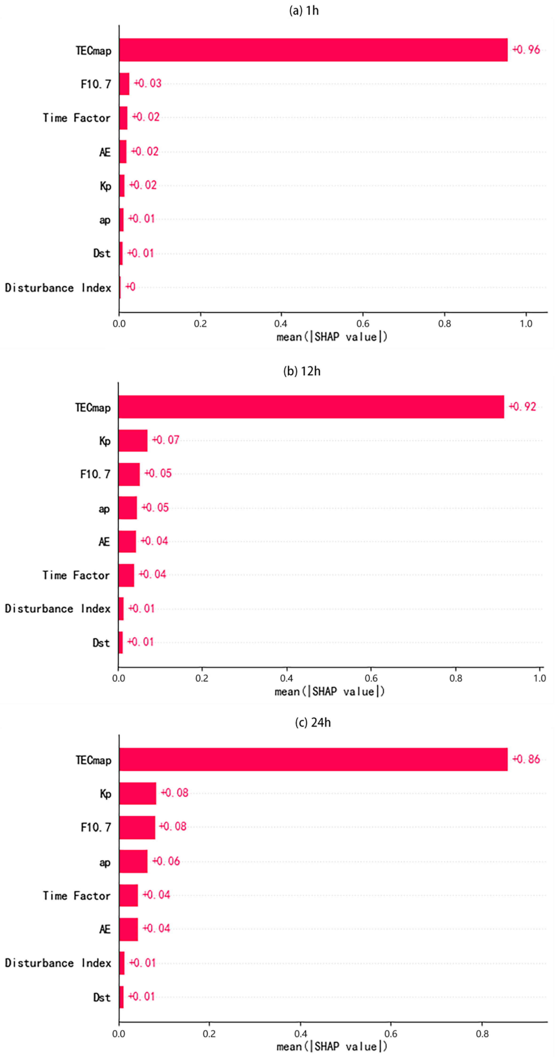
• According to the computed SHAP values during the model construction process, it is evident that historical TEC maps make the primary contribution to the prediction process. The contributions of F10.7, Kp, ap, AE, and the time factor follow next in significance, while the contributions of DI and Dst are minimal but still play a necessary role in improving accuracy. As the predicted length increases, the SHAP values of TEC maps gradually decrease, while the SHAP values of other features progressively increase. This indicates the indispensable roles played by the geomagnetic index, solar activity index, time factor, and DI in long-term predictions.
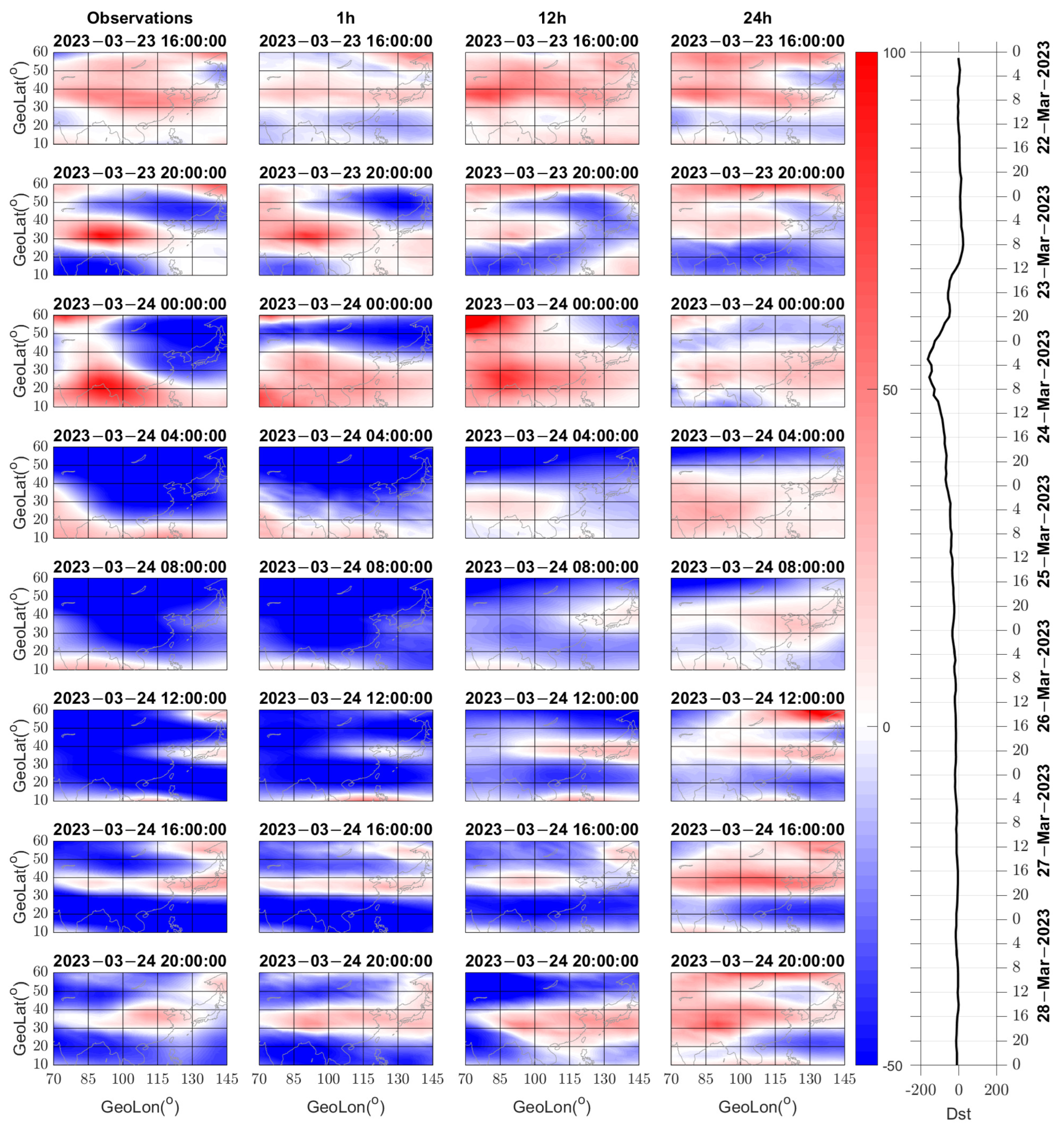
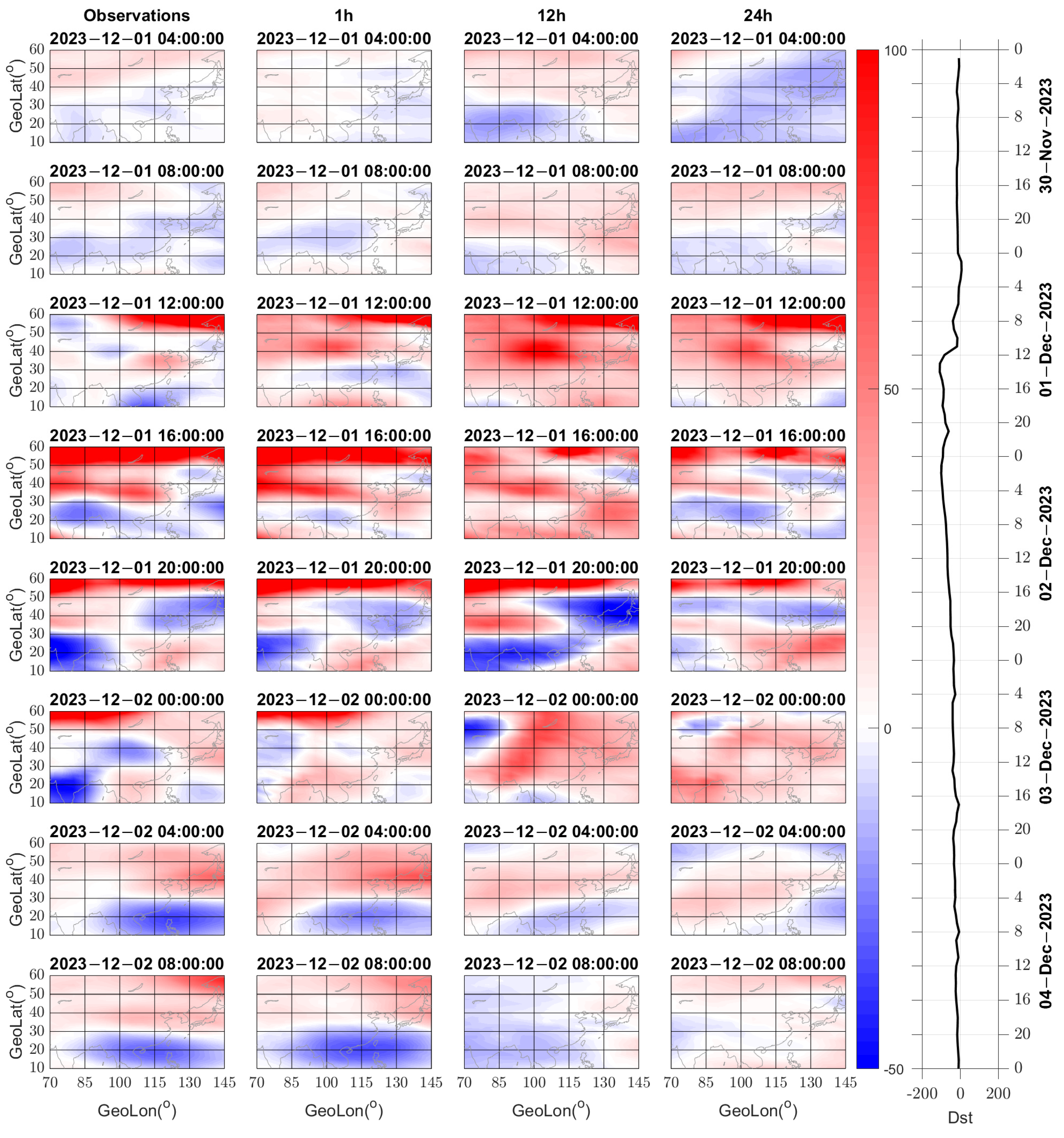
• Through the analysis of the prediction results, it is evident that the model performs well in short-term forecasts, accurately predicting the occurrence of ionospheric storms, the magnitude of disturbances, and their evolution. However, as the predicted length increases, the prediction accuracy of the model gradually decreases, and there may be a small number of incorrect predictions. Nevertheless, even with some errors, the model is still capable of capturing the entire process of ionospheric storms in the majority of events.
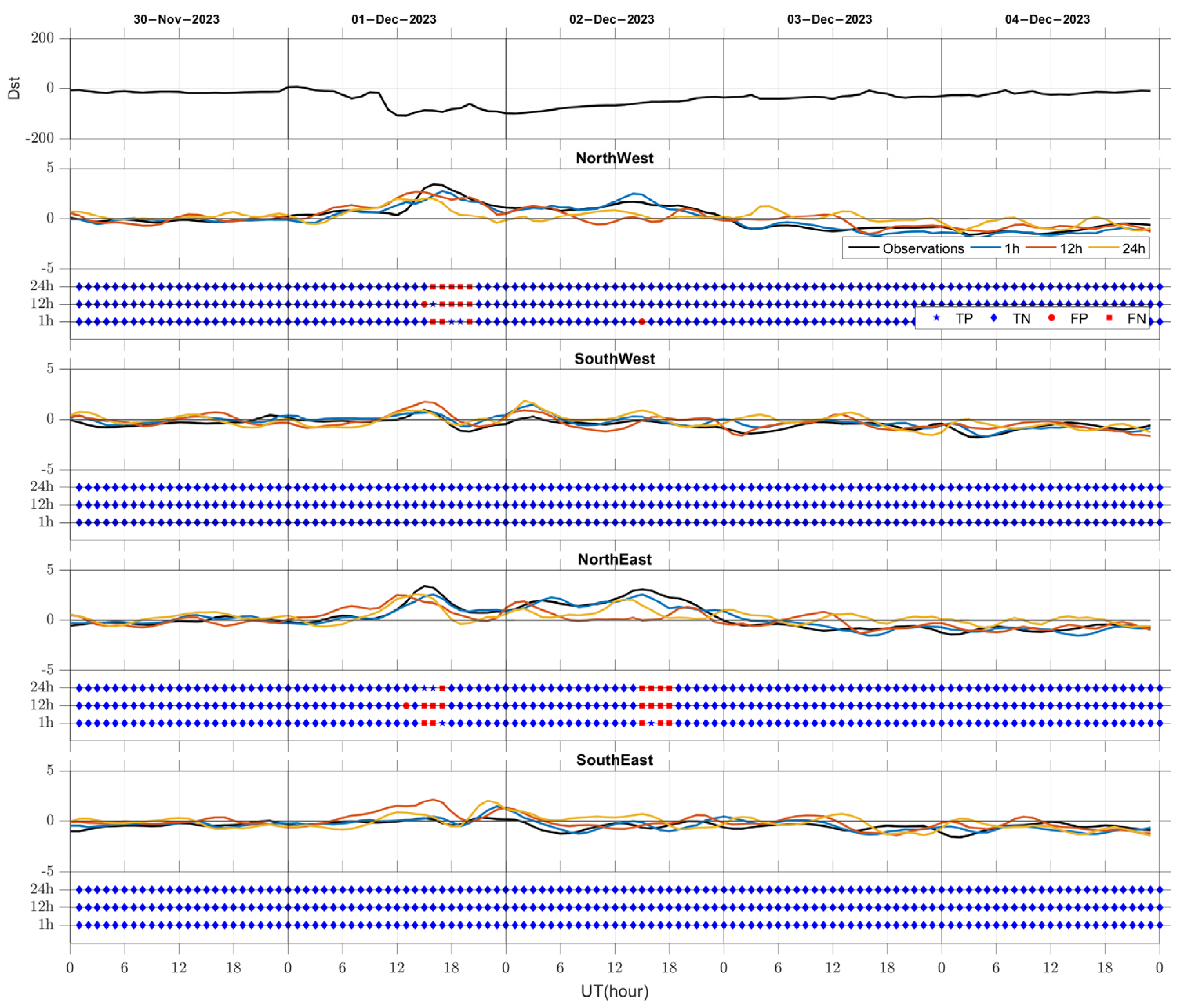
• When classifying ionospheric storms, the model may encounter classification errors in the initial stage of disturbances during short-term forecasts. However, it demonstrates accurate classification at other time points. In long-term predictions, although some errors may occur in the forecast results, they are primarily due to inaccuracies in predicting the magnitude of disturbances. Nonetheless, the overall trends and evolution processes are correctly identified by the model.
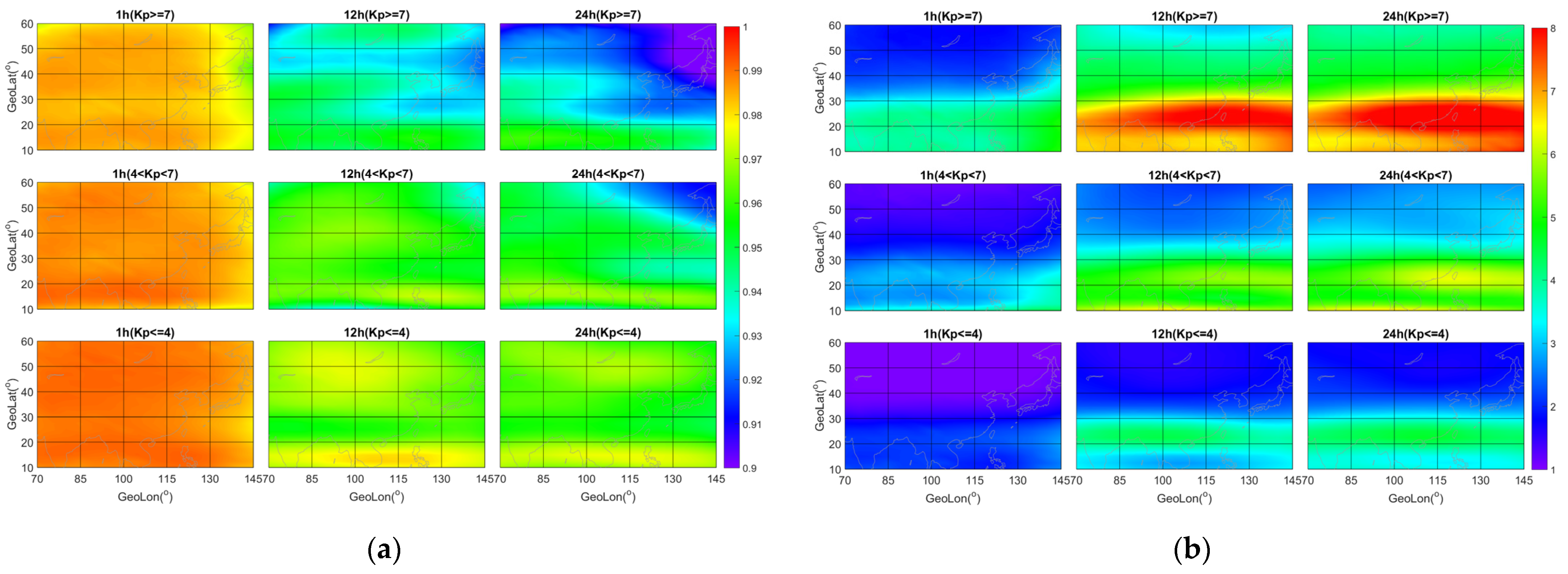
• In the prediction results, the relative error in the northeast region is higher compared to the southwest region, while the absolute error is not significant. In terms of classification evaluation, the northern region exhibits lower accuracy but higher F1 scores compared to the southern region. These differences may be attributed to variations in the occurrence rate and magnitude of ionospheric storms among different regions. The northeast region experiences a higher occurrence rate of negative storms and stronger disturbances, whereas the opposite is true for the southwest region. These factors could contribute to the varying prediction performance of the model in different regions.

The proposed Mixed CNN-BiLSTM model has achieved promising results in the prediction and classification of ionospheric storms in China. However, further improvements are necessary, particularly for the northeast region and cases of negative storms. Future research could explore the incorporation of additional features specific to these regions and refine the model architecture to more effectively capture the patterns of ionospheric variations.

References

1. Basu, S.; Basu, S.; MacKenzie, E.; Coley, W.R.; Sharber, J.R.; Hoegy, W.R. Plasma structuring by the gradient drift instability at high latitudes and comparison with velocity shear driven processes. J. Geophys. Res. Space Phys. 2012, 95, 7799–7818. [Google Scholar] [CrossRef]
2. Jakowski, N.; Béniguel, Y.; De Franceschi, G.; Pajares, M.H.; Jacobsen, K.S.; Stanislawska, I.; Tomasik, L.; Warnant, R.; Wautelet, G. Monitoring, tracking and forecasting ionospheric perturbations using GNSS techniques. J. Space Weather Space Clim. 2012, 2, A22. [Google Scholar] [CrossRef]
3. Klobuchar, J.A. Ionospheric time-delay algorithm for single-frequency GPS users. IEEE Trans. Aerosp. Electron. Syst. 1987, 3, 325–331. [Google Scholar] [CrossRef]
4. Prieto-Cerdeira, R.; Orús-Pérez, R.; Breeuwer, E.; Lucas-Rodriguez, R.; Falcone, M. Performance of the Galileo Single-Frequency Ionospheric Correction During In-Orbit Validation. GPS World 2014, 25, 53–58. [Google Scholar]
5. Yuan, Y.; Wang, N.; Li, Z.; Huo, X. The BeiDou global broadcast ionospheric delay correction model (BDGIM) and its preliminary performance evaluation results. Navigation 2019, 66, 55–69. [Google Scholar] [CrossRef]
6. Prölss, G.W. Ionospheric F-region storms. In Handbook of Atmospheric Electrodynamics; CRC Press: Boca Raton, FL, USA, 1995; Volume II. [Google Scholar]
7. Buonsanto, M.J.; González, S.A.; Lu, G.; Reinisch, B.W.; Thayer, J.P. Coordinated incoherent scatter radar study of the January 1997 storm. J. Geophys. Res. Space Phys. 1999, 104, 24625–24637. [Google Scholar] [CrossRef]
8. Mendillo, M. Storms in the ionosphere: Patterns and processes for total electron content. Rev. Geophys. 2006, 44, RG4001. [Google Scholar] [CrossRef]
9. Fuller-Rowell, T.J.; Codrescu, M.V.; Moffett, R.J.; Quegan, S. Response of the thermosphere and ionosphere to geomagnetic storms. J. Geophys. Res. Space Phys. 1994, 99, 3893–3914. [Google Scholar] [CrossRef]
10. Fuller-Rowell, T.J.; Codrescu, M.V.; Rishbeth, H.; Moffett, R.J.; Quegan, S. On the seasonal response of the thermosphere and ionosphere to geomagnetic storms. J. Geophys. Res. Space Phys. 1996, 101, 2343–2353. [Google Scholar] [CrossRef]
11. Matamba, T.M.; Habarulema, J.B. Ionospheric Responses to CME- and CIR-Driven Geomagnetic Storms Along 30°E–40°E Over the African Sector From 2001 to 2015. Space Weather 2018, 16, 538–556. [Google Scholar] [CrossRef]
12. Blanc, M.; Richmond, A.D. The Ionospheric Disturbance Dynamo. J. Geophys. Res. Space Phys. 1980, 85, 1669–1686. [Google Scholar] [CrossRef]
13. Camporeale, E. The Challenge of Machine Learning in Space Weather: Nowcasting and Forecasting. Space Weather 2019, 17, 1166–1207. [Google Scholar] [CrossRef]
14. Buonsanto, M.J. Ionospheric storms—A review. Space Sci. Rev. 1999, 88, 563–601. [Google Scholar] [CrossRef]
15. Vijaya Lekshmi, D.; Balan, N.; Tulasi Ram, S.; Liu, J.Y. Statistics of geomagnetic storms and ionospheric storms at low and mid latitudes in two solar cycles. J. Geophys. Res. Space Phys. 2011, 116, 1–13. [Google Scholar] [CrossRef]
16. Akala, A.O.; Rabiu, A.B.; Somoye, E.O.; Oyeyemi, E.O.; Adeloye, A.B. The response of African equatorial GPS-TEC to intense geomagnetic storms during the ascending phase of solar cycle 24. J. Atmos. Sol. Terr. Phys. 2013, 98, 50–62. [Google Scholar] [CrossRef]
17. Araujo-Pradere, E.A.; Fuller-Rowell, T.J.; Codrescu, M.V. STORM: An empirical storm-time ionospheric correction model 1. Model description. Radio Sci. 2002, 37, 3-1–3-12. [Google Scholar] [CrossRef]
18. Araujo-Pradere, E.A.; Fuller-Rowell, T.J. STORM: An empirical storm-time ionospheric correction model 2. Validation. Radio Sci. 2002, 37, 1–14. [Google Scholar] [CrossRef]
19. Araujo-Pradere, E.A.; Fuller-Rowell, T.J.; Bilitza, D. Time Empirical Ionospheric Correction Model (STORM) response in IRI2000 and challenges for empirical modeling in the future. Radio Sci. 2004, 39, 1–8. [Google Scholar] [CrossRef]
20. Kutiev, I.; Muhtarov, P. Modeling of midlatitude F region response to geomagnetic activity. J. Geophys. Res. Space Phys. 2001, 106, 15501–15509. [Google Scholar] [CrossRef]
21. Kutiev, I.; Muhtarov, P. Empirical modeling of global ionospheric foF2 response to geomagnetic activity. J. Geophys. Res. Space Phys. 2003, 108, SIA 5-1–SIA 5-11. [Google Scholar] [CrossRef]
22. Kutiev, I.; Muhtarov, P. Modeling the storm-time deviations of foF2 on a global scale. Adv. Space Res. 2004, 33, 910–916. [Google Scholar] [CrossRef]
23. Mukhtarov, P.; Andonov, B.; Pancheva, D. Global empirical model of TEC response to geomagnetic activity. J. Geophys. Res. Space Phys. 2013, 118, 6666–6685. [Google Scholar] [CrossRef]
24. Mukhtarov, P.; Pancheva, D.; Andonov, B.; Pashova, L. Global TEC maps based on GNNS data: 2. Model evaluation. J. Geophys. Res. Space Phys. 2013, 118, 4609–4617. [Google Scholar] [CrossRef]
25. Mukhtarov, P.; Pancheva, D.; Andonov, B.; Pashova, L. Global TEC maps based on GNSS data: 1. Empirical background TEC model. J. Geophys. Res. Space Phys. 2013, 118, 4594–4608. [Google Scholar] [CrossRef]
26. Tsagouri, I.; Belehaki, A. A new empirical model of middle latitude ionospheric response for space weather applications. Adv. Space Res. 2006, 37, 420–425. [Google Scholar] [CrossRef]
27. Tsagouri, I.; Belehaki, A. An upgrade of the solar-wind-driven empirical model for the middle latitude ionospheric storm-time response. J. Atmos. Sol. Terr. Phys. 2008, 70, 2061–2076. [Google Scholar] [CrossRef]
28. Tsagouri, I.; Koutroumbas, K.; Belehaki, A. Ionospheric foF2 forecast over Europe based on an autoregressive modeling technique driven by solar wind parameters. Radio Sci. 2009, 44, 1–21. [Google Scholar] [CrossRef]
29. Tsagouri, I.; Koutroumbas, K.; Elias, P. A new short-term forecasting model for the total electron content storm time disturbances. J. Space Weather Space Clim. 2018, 8, A33. [Google Scholar] [CrossRef]
30. Cander, L.R. Artificial neural network applications in ionospheric studies. Ann. Geophys. 1998, 41, 757–766. [Google Scholar] [CrossRef]
31. McKinnell, L.A.; Poole, A.W.V. A neural network based electron density model for the E layer. Adv. Space Res. 2003, 31, 589–595. [Google Scholar] [CrossRef]
32. McKinnell, L.A.; Friedrich, M.; Steiner, R.J. A new approach to modelling the daytime lower ionosphere at auroral latitudes. Adv. Space Res. 2004, 34, 1943–1948. [Google Scholar] [CrossRef]
33. McKinnell, L.A.; Poole, A.W.V. Predicting the ionospheric F layer using neural networks. J. Geophys. Res. Space Phys. 2004, 109, A08308. [Google Scholar] [CrossRef]
34. Tulunay, Y.; Tulunay, E.; Senalp, E.T. The neural network technique––1: A general exposition. Adv. Space Res. 2004, 33, 983–987. [Google Scholar] [CrossRef]
35. Tulunay, Y.; Tulunay, E.; Senalp, E.T. The neural network technique––2: An ionospheric example illustrating its application. Adv. Space Res. 2004, 33, 988–992. [Google Scholar] [CrossRef]
36. Tulunay, E.; Senalp, E.T.; Radicella, S.M.; Tulunay, Y. Forecasting total electron content maps by neural network technique. Radio Sci. 2006, 41, 1–12. [Google Scholar] [CrossRef]
37. Sai Gowtam, V.; Tulasi Ram, S. An Artificial Neural Network-Based Ionospheric Model to Predict NmF2 and hmF2 Using Long-Term Data Set of FORMOSAT-3/COSMIC Radio Occultation Observations: Preliminary Results. J. Geophys. Res. Space Phys. 2017, 122, 11743–11755. [Google Scholar] [CrossRef]
38. Tulasi Ram, S.; Sai Gowtam, V.; Mitra, A.; Reinisch, B. The Improved Two-Dimensional Artificial Neural Network-Based Ionospheric Model (ANNIM). J. Geophys. Res. Space Phys. 2018, 123, 5807–5820. [Google Scholar] [CrossRef]
39. Uwamahoro, J.C.; Habarulema, J.B. Modelling total electron content during geomagnetic storm conditions using empirical orthogonal functions and neural networks. J. Geophys. Res. Space Phys. 2015, 120, 11,000–11,012. [Google Scholar] [CrossRef]
40. Tebabal, A.; Radicella, S.M.; Nigussie, M.; Damtie, B.; Nava, B.; Yizengaw, E. Local TEC modelling and forecasting using neural networks. J. Atmos. Sol. Terr. Phys. 2018, 172, 143–151. [Google Scholar] [CrossRef]
41. Moon, S.; Kim, Y.H.; Kim, J.-H.; Kwak, Y.-S.; Yoon, J.-Y. Forecasting the ionospheric F2 Parameters over Jeju Station (33.43°N, 126.30°E) by Using Long Short-Term Memory. J. Korean Phys. Soc. 2020, 77, 1265–1273. [Google Scholar] [CrossRef]
42. Kim, J.H.; Kwak, Y.S.; Kim, Y.; Moon, S.I.; Jeong, S.H.; Yun, J. Potential of Regional Ionosphere Prediction Using a Long Short-Term Memory Deep-Learning Algorithm Specialized for Geomagnetic Storm Period. Space Weather 2021, 19, e2021SW002741. [Google Scholar] [CrossRef]
43. Chen, Z.; Liao, W.; Li, H.; Wang, J.; Deng, X.; Hong, S. Prediction of Global Ionospheric TEC Based on Deep Learning. Space Weather 2022, 20, e2021SW002854. [Google Scholar] [CrossRef]
44. Chen, Z.; Wang, K.; Li, H.; Liao, W.; Tang, R.; Wang, J.s.; Deng, X. Storm-Time Characteristics of Ionospheric Model (MSAP) Based on Multi-Algorithm Fusion. Space Weather 2024, 22, e2022SW003360. [Google Scholar] [CrossRef]
45. Liu, L.; Morton, Y.J.; Liu, Y. ML Prediction of Global Ionospheric TEC Maps. Space Weather 2022, 20, e2022SW003135. [Google Scholar] [CrossRef]
46. Xia, G.; Zhang, F.; Wang, C.; Zhou, C. ED-ConvLSTM: A Novel Global Ionospheric Total Electron Content Medium-Term Forecast Model. Space Weather 2022, 20, e2021SW002959. [Google Scholar] [CrossRef]
47. Luo, H.; Gong, Y.; Chen, S.; Yu, C.; Yang, G.; Yu, F.; Hu, Z.; Tian, X. Prediction of Global Ionospheric Total Electron Content (TEC) Based on SAM-ConvLSTM Model. Space Weather 2023, 21, e2023SW003707. [Google Scholar] [CrossRef]
48. Sun, W.; Xu, L.; Huang, X.; Zhang, W.; Yuan, T.; Yan, Y. Bidirectional LSTM for ionospheric vertical Total Electron Content (TEC) forecasting. In Proceedings of the 2017 IEEE Visual Communications and Image Processing (VCIP), St. Petersburg, FL, USA, 10–13 December 2017; pp. 1–4. [Google Scholar]
49. Wang, H.; Liu, H.; Yuan, J.; Le, H.; Shan, W.; Li, L. MAOOA-Residual-Attention-BiConvLSTM: An Automated Deep Learning Framework for Global TEC Map Prediction. Space Weather 2024, 22, e2024SW003954. [Google Scholar] [CrossRef]
50. Yuan, Y.; Xia, G.; Zhang, X.; Zhou, C. Synthesis-Style Auto-Correlation-Based Transformer: A Learner on Ionospheric TEC Series Forecasting. Space Weather 2023, 21, e2023SW003472. [Google Scholar] [CrossRef]
51. Shih, C.Y.; Lin, C.Y.t.; Lin, S.Y.; Yeh, C.H.; Huang, Y.M.; Hwang, F.N.; Chang, C.H. Forecasting of Global Ionosphere Maps with Multi-Day Lead Time Using Transformer-Based Neural Networks. Space Weather 2024, 22, e2023sw003579. [Google Scholar] [CrossRef]
52. Li, Z.; Yuan, Y.; Wang, N.; Hernandez-Pajares, M.; Huo, X. SHPTS: Towards a new method for generating precise global ionospheric TEC map based on spherical harmonic and generalized trigonometric series functions. J. Geod. 2014, 89, 331–345. [Google Scholar] [CrossRef]
53. Ioffe, S.; Szegedy, C. Batch normalization: Accelerating deep network training by reducing internal covariate shift. Int. Conf. Mach. Learn. 2015, arXiv:1502.03167. [Google Scholar] [CrossRef]
54. Hochreiter, S.; Schmidhuber, J. Long short-term memory. Neural Comput. 1997, 9, 1735–1780. [Google Scholar] [CrossRef] [PubMed]
55. Schuster, M.; Paliwal, K.K. Bidirectional recurrent neural networks. IEEE Trans. Signal Process. 1997, 45, 2673–2681. [Google Scholar] [CrossRef]
56. Lundberg, S.M.; Lee, S.I. A unified approach to interpreting model predictions. Adv. Neural Inf. Process. Syst. 2017, 30, 4765–4774. [Google Scholar] [CrossRef]
57. Ban, P.; Guo, L.; Zhao, Z.; Sun, S.; Zhang, H.; Wang, F.; Xu, Z.; Sun, F.; Xu, T. A New Index to Descript the Regional Ionospheric Disturbances During Storm Time. J. Geophys. Res. Space Phys. 2022, 127, e2021JA030126. [Google Scholar] [CrossRef]
58. Liu, J.; Zhao, B.; Liu, L. ime delay and duration of ionospheric total electron content. Ann. Geophys. 2010, 28, 795–805. [Google Scholar] [CrossRef]
59. Kataoka, R.; Miyoshi, Y.; Shiokawa, K.; Nishitani, N.; Keika, K.; Amano, T.; Seki, K. Magnetic Storm-Time Red Aurora as Seen From Hokkaido, Japan on 1 December 2023 Associated With High-Density Solar Wind. Geophys. Res. Lett. 2024, 51, e2024GL108778. [Google Scholar] [CrossRef]
60. Zhao, B.; Yang, C.; Cai, Y.; Jin, Y.; Liang, Y.; Ding, F.; Yue, X.; Wan, W. East-West Difference in the Ionospheric Response of the March 1989 Great Magnetic Storm Throughout East Asian Region. J. Geophys. Res. Space Phys. 2019, 124, 9364–9380. [Google Scholar] [CrossRef]
61. Ren, X.; Zhao, B.; Ren, Z.; Wang, Y.; Xiong, B. Deep Learning-Based Prediction of Global Ionospheric TEC During Storm Periods: Mixed CNN-BiLSTM Method. Space Weather 2024, 22, e2024SW003877. [Google Scholar] [CrossRef]
Figure 1. The structure of Mixed CNN-BiLSTM.
Remotesensing 16 03160 g001
Figure 2. SHAP values for different predicted lengths.
Remotesensing 16 03160 g002
Figure 3. Evolution process of predicted and observed values of RTEC during the geomagnetic storm on 24 March 2023.
Remotesensing 16 03160 g003
Figure 4. PI of predicted and observed values during the geomagnetic storm on 23 March 2023.
Remotesensing 16 03160 g004
Figure 5. Evolution process of predicted and observed values of RTEC during the geomagnetic storm on 1 December 2023.
Remotesensing 16 03160 g005
Figure 6. PI of predicted and observed values during the geomagnetic storm on 1 December 2023.
Remotesensing 16 03160 g006
Figure 7. Comparison of prediction accuracy for different geomagnetic environments and predicted length. (a) The prediction accuracy index is R 2 . (b) The prediction accuracy index is RMSE.
Remotesensing 16 03160 g007