Multiview Multistatic vs. Multimonostatic Three-Dimensional Ground-Penetrating Radar Imaging: A Comparison

Abstract

The availability of multichannel ground-penetrating radar systems capable of gathering multiview, multistatic, multifrequency data provides novel chances to improve subsurface imaging results. However, customized data processing techniques and smart choices of the measurement setup are needed to find a trade-off between image quality and acquisition time. In this paper, we adopt a Born Approximation-based full 3D approach, which can manage multiview-multistatic, multifrequency data and faces the imaging as a linear inverse scattering problem. The inverse problem is solved by exploiting the truncated singular value decomposition as a regularization scheme. The paper presents a theoretical study aimed at assessing how the reconstruction capabilities of the imaging approach depend on the adopted measurement configuration. In detail, the performance achievable in the standard case of multimonostatic, multifrequency data is compared with that provided by a multiview-multistatic, multifrequency configuration, where the data are gathered by considering a progressively increasing number of transmitting antennas. The comparison of the achievable imaging performance is carried out by exploiting the spectral content and the point spread function, which are general tools to foresee the achievable reconstruction capabilities. Reconstruction results related to a numerical experiment based on full-wave data are also provided.

1. Introduction

The Earth’s subsurface exploration has intrigued scientists and professionals for years, offering insights into hidden landscapes, buried structures, and ancient artifacts. Ground-penetrating radar (GPR) plays a crucial role in this endeavor, offering a non-invasive and detailed view of subsurface features [1,2] and, indeed, it finds wide application in various contexts, ranging from environmental monitoring and civil engineering projects [3,4,5] to archaeological surveys and geological investigations [6,7].

Thanks to its recognized usefulness, GPR technology is the subject of continuous technological advancements aimed at improving both data collection and data processing aspects. In this frame, multichannel systems are today standard tools to collect data along multiple profiles simultaneously, and thus speed up the measurement stage. On the other hand, the use of Multiple Input Multiple Output GPR (MIMO GPR) is receiving attention because, compared with multimonostatic systems, it collects an increased amount of data, resulting in an improved target detection and reconstruction accuracy [8,9,10,11]. Indeed, in the case of MIMO GPR, the data acquisition can be planned in such a way that two or more antennas act as transmitters and, for each transmitting antenna, the scattered field data are collected by different receiving antennas. Of course, several measurement configurations made up of a different number of transmitting (Tx) and receiving (Rx) antennas can be considered. For instance, the same number of Tx and Rx antennas can be adopted or fewer Tx antennas than RX ones can be used. In addition, different imaging capabilities are expected for different measurement setups.

MIMO GPR systems have been considered for demining [12,13,14] and Moon exploration [10,15,16,17,18] and require the design of data processing approaches capable of managing multiview-multistatic data and exploiting the increased amount of available information [19,20,21,22]. In this frame, microwave tomography (MWT) is a flexible tool easily adaptable to different measurement setups and reference scenarios [23,24].

Among MWT approaches, those based on the Born Approximation [25] have been applied successfully in a large number of real scenarios [26,27,28,29] and have proven to be effective whatever the measurement configuration and the scenario under test [23,30,31,32,33,34,35,36,37,38,39,40].

In this study, we consider a Born Approximation-based MWT approach able to perform a full 3D imaging of the scenario under test by taking in input from both multimonostatic and multiview-multistatic, multifrequency GPR data. Specifically, in the multiview-multistatic case, a hybrid measurement configuration is realized because multiview- multistatic data are gathered along the direction parallel to the antenna array, the x-axis in this paper, while multimonostatic data are collected along the array movement direction, herein the y-axis. The adopted approach faces the imaging as a linear inverse scattering problem, with models transmitting and receiving antennas as linearly polarized electric dipoles, and adopts the truncated singular value decomposition (TSVD) of the involved scattering operator as a regularized inversion scheme [41].

As a novel contribution, this paper investigates how the measurement setup impacts the imaging performance of the MWT approach. The task is pursued by using the spectral content and the point spread function as general tools to estimate the achievable reconstruction capabilities [2].

It is worth pointing out that the proposed analysis is general, i.e., it does not depend on the specific MIMO GPR system adopted to collect the data, and it provides theoretical indications on the expected reconstruction capabilities of the adopted MWT approach in real applications.

Results referring to full-wave synthetic data concerning an L-shaped buried cavity are provided to validate the expected performance in the case of an extended target. The proposed analysis accounts for an array made by a fixed number of evenly spaced antennas, which can be configured in such a way as to collect multimonostatic or multiview-multistatic multifrequency data. In the multiview-multistatic case, the number of Tx antennas is changed, while all the antennas of the GPR array act as receivers.

The paper is organized as follows: Section 2 presents the mathematical formulation of the problem. Section 3 analyzes the imaging capabilities in terms of spectral content and point spread function. In this respect, it should be stressed that the optimal regularization parameter of the TSVD is fixed by applying the L-curve technique [42,43]. Section 4 accounts for the achievable imaging capabilities through numerical results referring to an extended buried target. Section 5 provides the conclusions and addresses possible future research directions.

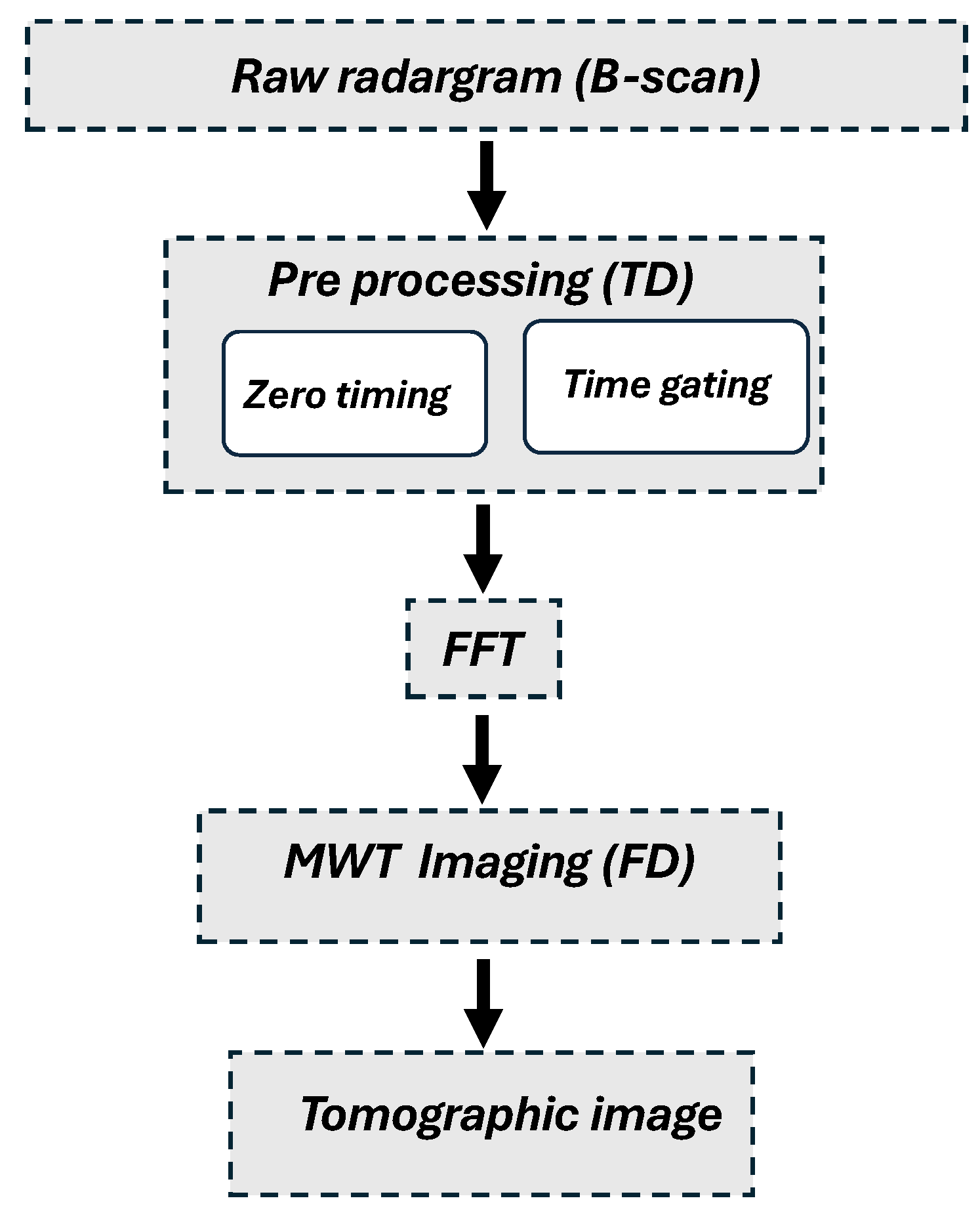
2. GPR Imaging Problem

Let us consider the reference scenario depicted in Figure 1, which shows the investigation domain $\mathcal{D}$ and a sketch of the GPR data collection configuration. This last is associated to a multichannel system made up by an array of $N_t$ transmitting (Tx) and $N_r$ receiving (Rx) antennas ($N_t\le N_r$) evenly distributed along the x-axis within the interval $X=[x_{min},x_{max}]$. The GPR is located in free space, closely adjacent to the soil surface and moves along the y-axis in the range $Y=[y_{min},y_{max}]$. At each position along the y-axis, the system records multimonostatic or multiview-multistatic, multifrequency data.

Let us recall that multimonostatic data are collected when the probing electromagnetic pulse is radiated by a transmitting antenna $T{x}_i$ and the backscattered field is measured only by the corresponding co-located receiving antenna $R{x}_i$. Conversely, multiview-multistatic data are gathered when, for each transmitting antenna $T{x}_i$ with $i=1,\dots ,N_t$, the backscattered field is measured by all the receiving antennas $R{x}_j$ with $j=1,\dots ,N_r$. The backscattered field is collected in the frequency band $B=\left[f_{min}{f}_{max}\right]$ for all the considered configurations.

It is also worth pointing out that, if a multiview-multistatic data acquisition is planned, by moving the GPR along the y-axis, a hybrid measurement configuration is achieved where data are multiview multistatic along x and multimonostatic along y.

The imaging is formulated as an inverse scattering problem by assuming that the unknown targets are located in a lossless homogeneous and non-magnetic ($\mu ={\mu }_0=1.25\times {10}^6$ H/m) soil characterized by the dielectric permittivity ${\epsilon }_s={\epsilon }_{rs}{\epsilon }_0$, with ${\epsilon }_{rs}$ being the soil relative permittivity and ${\epsilon }_0=8.85\times {10}^{-12}$ F/m the free-space permittivity. The targets are located in $\mathcal{D}$ and are modeled as dielectric anomalies with respect to the background soil. Accordingly, at the generic point $\mathbf{r}=(x,y,z)$ in $\mathcal{D}$, the presence of a target is described by the unknown contrast function:

$$\chi \left(\mathbf{r}\right)={\displaystyle \frac{\epsilon \left(\mathbf{r}\right)-{\epsilon }_s}{{\epsilon }_s}}$$

(1)

where $\epsilon \left(\mathbf{r}\right)$ is the target permittivity.

According to the Born Approximation and modeling the Tx and Rx antennas as Hertzian dipoles linearly polarized along the direction ${\mathbf{u}}_{Tx}$ and ${\mathbf{u}}_{Rx}$, the data-unknown relationship to be solved is given in the frequency domain by:

$$E_s({\mathbf{r}}_{\mathbf{t}},{\mathbf{r}}_{\mathbf{o}},\omega )={\mathbf{u}}_{Rx}·\int \int {\int }_{\mathcal{D}}\mathbf{G}(\mathbf{r},{\mathbf{r}}_{\mathbf{o}},\omega )·{\mathbf{E}}_{inc}({\mathbf{r}}_{\mathbf{t}},\mathbf{r},\omega )\chi \left(\mathbf{r}\right)\mathit{d}\mathbf{r}=\mathcal{A}\chi$$

(2)

where $\mathcal{A}$ is a linear projection operator, $E_s$ is the measured component of the backscattered field along ${\mathbf{u}}_{Rx}$, ${\mathbf{r}}_{\mathbf{t}}=(x_t,y_t,z_t)$, and ${\mathbf{r}}_{\mathbf{o}}=(x_o,y_o,z_o)$ denote the position of the Tx and Rx antennas, respectively, $\mathbf{G}(\mathbf{r},{\mathbf{r}}_{\mathbf{o}},\omega )$ is the dyadic Green’s function accounting for the radiation from $\mathbf{r}$ to ${\mathbf{r}}_{\mathbf{o}}$ at the angular frequency $\omega$, and ${\mathbf{E}}_{inc}({\mathbf{r}}_{\mathbf{t}},\mathbf{r},\omega )$ is the incident field at $\mathbf{r}$ due to the antenna located at ${\mathbf{r}}_{\mathbf{t}}$:

$${\mathbf{E}}_{inc}({\mathbf{r}}_{\mathbf{t}},\mathbf{r},\omega )=-j\omega {\mu }_0\mathbf{G}(\mathbf{r},{\mathbf{r}}_{\mathbf{t}},\omega )·{\mathbf{u}}_{Tx}$$

(3)

Under the far-field approximation and by taking into account that, being the antenna close to the air–soil interface, the signal propagation occurs into the soil mainly, the dyadic Green’s function $G(\mathbf{r},{\mathbf{r}}_{\mathbf{t},\mathbf{o}},\omega )$ can be written as [44]:

$$G(\mathbf{r},{\mathbf{r}}_{\mathbf{t},\mathbf{o}},\omega )={\displaystyle \frac{exp(-jk{R}_{t,o})}{4\pi R_{t,o}}}\left[\begin{array}{ccc}1-{\displaystyle \frac{{(x-x_{t,o})}^2}{R_{t,o}^2}}& -{\displaystyle \frac{(x-x_{t,o})(y-y_{t,o})}{R_{t,o}^2}}& -{\displaystyle \frac{(x-x_{t,o})(z-zt,o)}{R_{t,o}^2}}\\ -{\displaystyle \frac{(x-x_{t,o})(y-y_{t,o})}{R_{t,o}^2}}& 1-{\displaystyle \frac{{(y-y_{t,o})}^2}{R_{t,o}^2}}& -{\displaystyle \frac{(y-y_{t,o})(z-zt,o)}{R_{t,o}^2}}\\ -{\displaystyle \frac{(x-x_{t,o})(z-zt,o)}{R_{t,o}^2}}& -{\displaystyle \frac{(y-y_{t,o})(z-zt,o)}{R_{t,o}^2}}& 1-{\displaystyle \frac{{(z-z_{t,o})}^2}{R_{t,o}^2}}\end{array}\right]$$

(4)

where $k=\omega \sqrt{{\mu }_0{\epsilon }_s}$ is the propagation constant in the soil at the angular frequency $\omega$ and $R_{t,o}=|\mathbf{r}-{\mathbf{r}}_{t,o}|=\sqrt{{(x-x_{t,o})}^2+{(y-y_{t,o})}^2+{(z-z_{t,o})}^2}$.

The linear integral equation, Equation (2), is solved by using the truncated singular value decomposition (TVSD) as a regularized inversion scheme. Accordingly, its solution is expressed in a closed form as:

$$\chi ={\displaystyle \sum _{n=0}^{N_{\delta }}}{\displaystyle \frac{\langle E_s,u_n\rangle }{{\sigma }_n}}{v}_n.$$

(5)

where $u_n$ and $v_n$ represent the left and right singular functions of the operator $\mathcal{A}$ (see Equation (2)), respectively, ${\sigma }_n$ are the singular values arranged in descending order, and $\langle ·,·\rangle$ denotes the scalar product in data space. In Equation (5), the truncation threshold $N_{\delta }$ is the regularization parameter that should assure a suitable trade-off between the accuracy of the solution and the robustness to the noise. The magnitude of the retrieved contrast $\chi$ is a spatial map referred to as tomographic image.

The determination of the optimal value of $N_{\delta }$ is a challenge that is here effectively faced using the L-curve method [42,43]. The essence of the L-curve lies in its graphical representation of the trade-off between the norm of the solution ${\left|\right|\chi \left|\right|}^2$ and the norm of the residue $\left|\right|E_s-\mathcal{A}\chi {\left|\right|}^2$, as the regularization parameter varies. On a logarithmic scale, the L-curve typically exhibits an “L” shape, wherein the knee or corner of the curve provides the optimal regularization parameter, i.e., the value allowing the desired balance between accuracy and stability of the solution. In this work, a MATLAB package for the analysis and the solution of discrete ill-posed problems developed by Hansen [45] is exploited to determine the optimal truncation index.

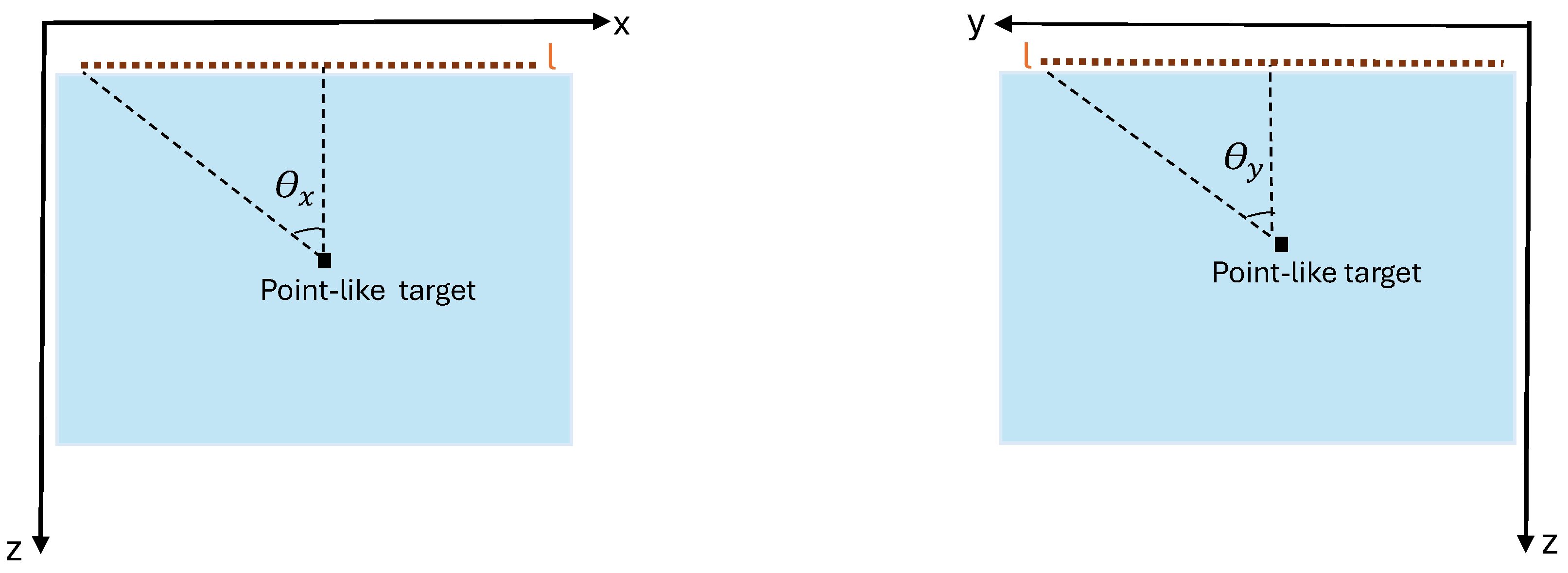
3. Resolution Analysis

3.1. Theoretical Background

The spectral content ($SC$) [2] and the point spread function ($PSF$) are the tools to analyze the filtering effects introduced by the linear integral operator $\mathcal{A}$ in Equation (2) and estimate the spatial resolution limits. As is well-known, $SC$ represents the retrievable global (average) harmonic content of the unknown obtained by accounting for all possible positions of the point target in $\mathcal{D}$. Conversely, the PSF embodies the reconstructed image of a point-like target and allows us to estimate the spatial resolution and how it changes with the target position.

Based on the SVD of $\mathcal{A}$, the spectral content is defined as:

$$\begin{array}{cc}\hfill & SC(k_x,k_y,k_z)=\hfill \\ \hfill & {\displaystyle \sum _{n=1}^{N_{\delta }}}{\left|{\widehat{v}}_n(k_x,k_y,k_z)\right|}^2={\displaystyle \sum _{n=1}^{N_{\delta }}}|\int \int {\int }_{\mathcal{D}}{v}_n(x,y,z)e^{-j(k_{x}x+k_{y}y+k_{z}z)}\mathrm{d}x\mathrm{d}y\mathrm{d}z{|}^2\hfill \end{array}$$

(6)

where $k_x$, $k_y$, $k_z$ are the spectral variables corresponding to x, y, z, respectively, and ${\widehat{v}}_n(k_x,k_y,k_z)$ is the 3D Fourier transform of the singular function $v_n(x,y,z)$.

In addition, under the TSVD regularization scheme, the point spread function is given by:

$$PSF(x,y,z)={\displaystyle \sum _{n=1}^{N_{\delta }}}{v}_n^{*}(x^{\prime },y^{\prime },z^{\prime })v_n(x,y,z)$$

(7)

where $(x^{\prime },y^{\prime },z^{\prime })$ denotes the position of the point-like target and ∗ the conjugation operation [41].

It is worth pointing out that $SC$ and $PSF$ in Equations (6) and (7) are general mathematical tools for forecasting the imaging performance of the TSVD-based linear microwave tomography approach, even in unconventional scenarios with different measurement domains and antenna setups (e.g., see [46,47,48]. However, since $\mathcal{A}$ depends on the scenario under test as well as on the adopted measurement configuration, $SC$ and $PSF$ must be computed numerically for the specific case at hand.

In the following, $SC$ and $PSF$ are considered to compare the imaging performance referring to the commonly adopted multimonostatic measurement configuration and those achievable with a multiview-multistatic data acquisition. Moreover, for a given antenna array system, they are exploited to establish the suitable number of transmitting antennas to be considered in the multiview-multistatic acquisition, provided that all the antennas in the GPR array act as receivers.

For the sake of comparison, we recall that for a multimonostatic, multifrequency configuration, the theoretical resolution limits are approximated by [26]:

$$\begin{array}{cc}\hfill & \Delta x={\displaystyle \frac{c_0}{4f_c\sqrt{{\epsilon }_s}sin{\theta }_x}}\hfill \\ \hfill & \Delta y={\displaystyle \frac{c_0}{4f_c\sqrt{{\epsilon }_s}sin{\theta }_y}}\hfill \\ \hfill & \Delta z={\displaystyle \frac{c_0}{2B\sqrt{{\epsilon }_s}}}\hfill \end{array}$$

(8)

Here, $\Delta x$, $\Delta y$, and $\Delta z$ represent the resolutions along the x, y, and z axes, respectively; $f_c$ denotes the central frequency in Hz, while ${\theta }_x$ and ${\theta }_y$ indicate the maximum illumination angles subtended by the measurement aperture with respect to the x and y axes, respectively (see Figure 2). Additionally, B stands for the radar bandwidth in Hz.

It must be stressed that closed resolution formulas are not available for the multiview-multistatic configuration addressed in this work, and then a numerical analysis is performed to assess the resolution limits as described in the following Subsection.

3.2. Resolution Analysis

$SC$ and $PSF$ are evaluated to investigate how the measurement configuration affects the imaging capabilities. The numerical analysis is carried out for a fixed investigation domain and multichannel GPR system. As shown in Figure 1, the GPR antenna array is made by eight Tx/Rx radiating elements evenly spaced by $7.5$ cm and collects data in the frequency band $B=[1.6,2.2]$ GHz (the central frequency is $f_c=1.9$ GHz and the uniform frequency step is $\delta f=68$ MHz). The antenna array is parallel to the x-axis and is moved with a 2 cm spatial offset along the y-axis, according to the coordinate reference system in Figure 1. The investigation domain has size $[0.2,0.8]\times [0.1,0.4]\times [0,0.6]$ m³. The soil relative permittivity is ${\epsilon }_{rs}=4$, reflecting typical soil conditions [1].

Beyond the multimonostatic configuration (here referred to as MM/MF), three multiview-multistatic setups, differing for the number of Tx antennas $N_t$, are considered (see Figure 3):

$$\left\{\begin{array}{cc}case1:\hfill & N_t=2,\hfill \\ case2:\hfill & N_t=4,\hfill \\ case3:\hfill & N_t=8,\hfill \end{array}\right.$$

(9)

while the number of receiving antennas $N_r$ does not change ($N_r=8$).

The curves in Figure 4 show the singular values of the operator $\mathcal{A}$ relevant to the four considered measurement configurations. As expected, the curves exhibit a rapid decay as the truncation index grows, and the curve referred to the MM/MF configuration experiences a faster decay than Case 2 and 3. On the other hand, the curve related to Case 1 shows a slightly faster decay than MM/MF in the interval $N_{\delta }<327$, after which an opposite trend is observed. In general, the curves of the multiview-multistatic setup suggest that, for a fixed TSVD threshold, the number of the singular values above the threshold increases with the number of Tx antennas and, accordingly, better imaging capabilities are expected.

The following analysis is carried out for different noise levels on the scattered field data. In particular, the data are corrupted by Additive White Gaussian Noise (AWGN) with a fixed signal-to-noise ratio (SNR). The TSVD regularization parameter $N_{\delta }$ is found using the L-curve method, as said in Section 2, and its values for SNRs ranging from 0 to 50 dB are listed in

Table 1. Optimal TSVD truncation index provided by L-Curve method for each configuration and SNR.

	SNR [dB]	0	5	10	15	20	25	30	35	40	50
Case 1	$N_{\delta }$	605	714	866	994	1095	1194	1306	1404	1476	1648
Case 2	$N_{\delta }$	929	1077	1317	1488	1655	1844	1999	2169	2333	2600
Case 3	$N_{\delta }$	1008	1138	1474	1741	1963	2176	2415	2570	2797	3157
MM/MF	$N_{\delta }$	338	530	567	723	756	796	847	887	916	973

.

Based on the results in Table 1, it can be concluded that, for a fixed configuration, the SNR increases with the number of singular functions, thus reducing the filtering effect of the TSVD. Additionally, for a given SNR, increasing the number of Tx antennas in the MIMO configurations also increases the number of singular values. Finally, the MM/MF configuration consistently exhibits a lower truncation index compared to the MIMO configurations. As an example, Figure 5 shows the behavior of the L-curves for each considered measurement configuration when $SNR=15$ dB. Such an SNR value is considered for the following computation of the $SC$ and $PSF$.

Figure 6 shows the cuts in the $k_x-k_z$ and $k_y-k_z$ planes of $SC$ obtained through Equation (6) for the considered measurement configurations. In agreement with the results of linear inverse scattering (e.g., see [2,35]), the scattering operator $\mathcal{A}$ acts as a low pass filter along the x and y directions, i.e., along the directions defining the measurement plane, while it operates as a bandpass filtering along the z-axis for every measurement configuration.

To estimate the achievable spatial resolution, we evaluate the $PSF$ for a point target located at the center of the investigation domain, i.e., at $(0.5,0.25,0.3)$ m. The cuts along x, y, and z of the PSF amplitude normalized to the maximum are compared in Figure 7a, Figure 7b, Figure 7c, respectively. The figures reveal comparable spatial resolutions (i.e., main lobe width) along x and y with all configurations; however, the MM/MF configuration is characterized by a notable increase in the sidelobes along the array direction (x-axis). This outcome is an effect of the chosen spacing among the antenna of the array (i.e., $7.5$ cm), which is nearly equal to the wavelength in the considered soil at the center frequency. On the other hand, all the MIMO configurations at hand allow mitigating this problem by suppressing the sidelobes. As regards the PSF cut along depth (see Figure 7c), similar resolutions are achieved with all configurations, save for Case 1 showing a slight broadening of the PSF main lobe. The spatial resolution values evaluated according to the half-power (i.e., $-3$ dB) criterion and reported in

Table 2. Resolution results for a point-like target placed at (0.2, 0.25, 0.1) m related to the considered cases.

Resolution	Theoretical (MM/MF) [m]	Case 1 [m]	Case 2 [m]	Case 3 [m]	MM/MF [m]
${\Delta }_x$	0.02	0.02	0.02	0.02	0.02
${\Delta }_y$	0.04	0.04	0.04	0.04	0.04
${\Delta }_z$	0.1	0.1	0.08	0.08	0.08

confirm the former statements.

It is also stressed that since resolution limits in Case 2 and Case 3 look very similar to each other, it is reasonable to consider $N_t=4$ Tx antennas as a suitable trade-off between the imaging improvement and the measurement time.

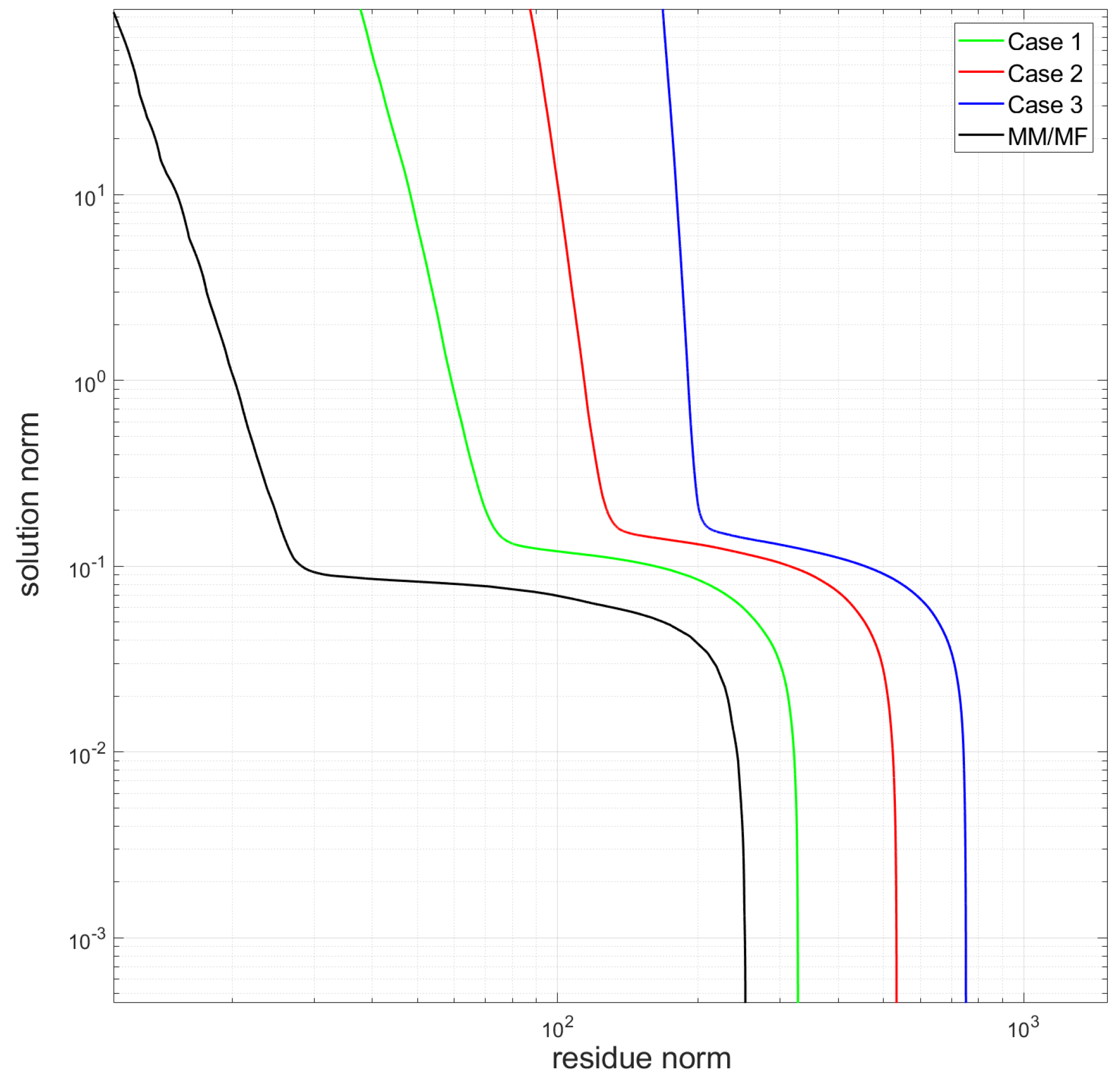
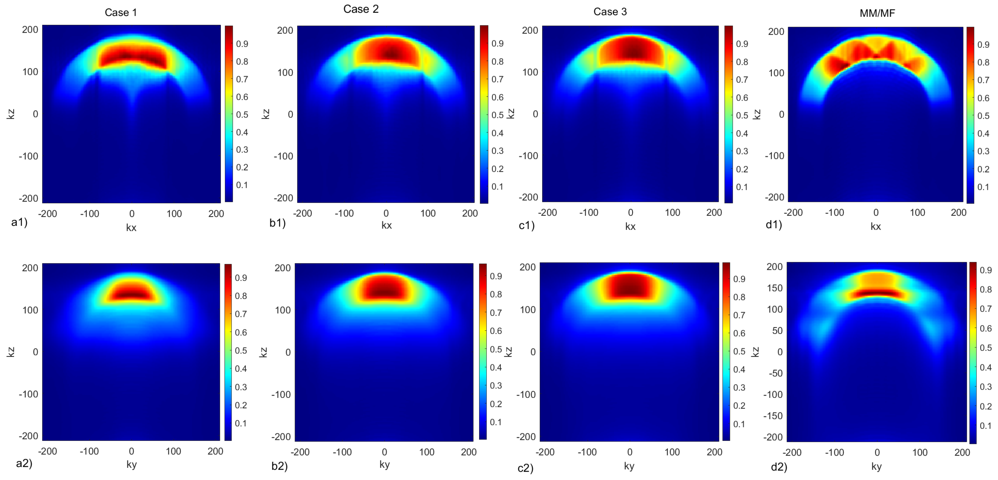
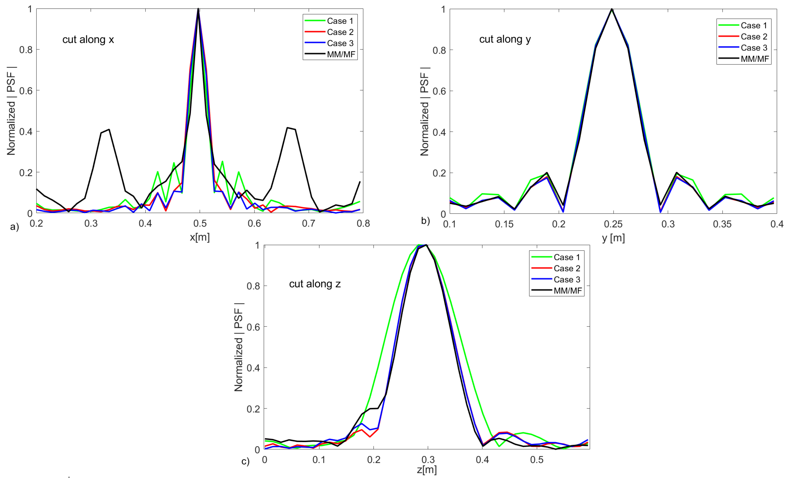
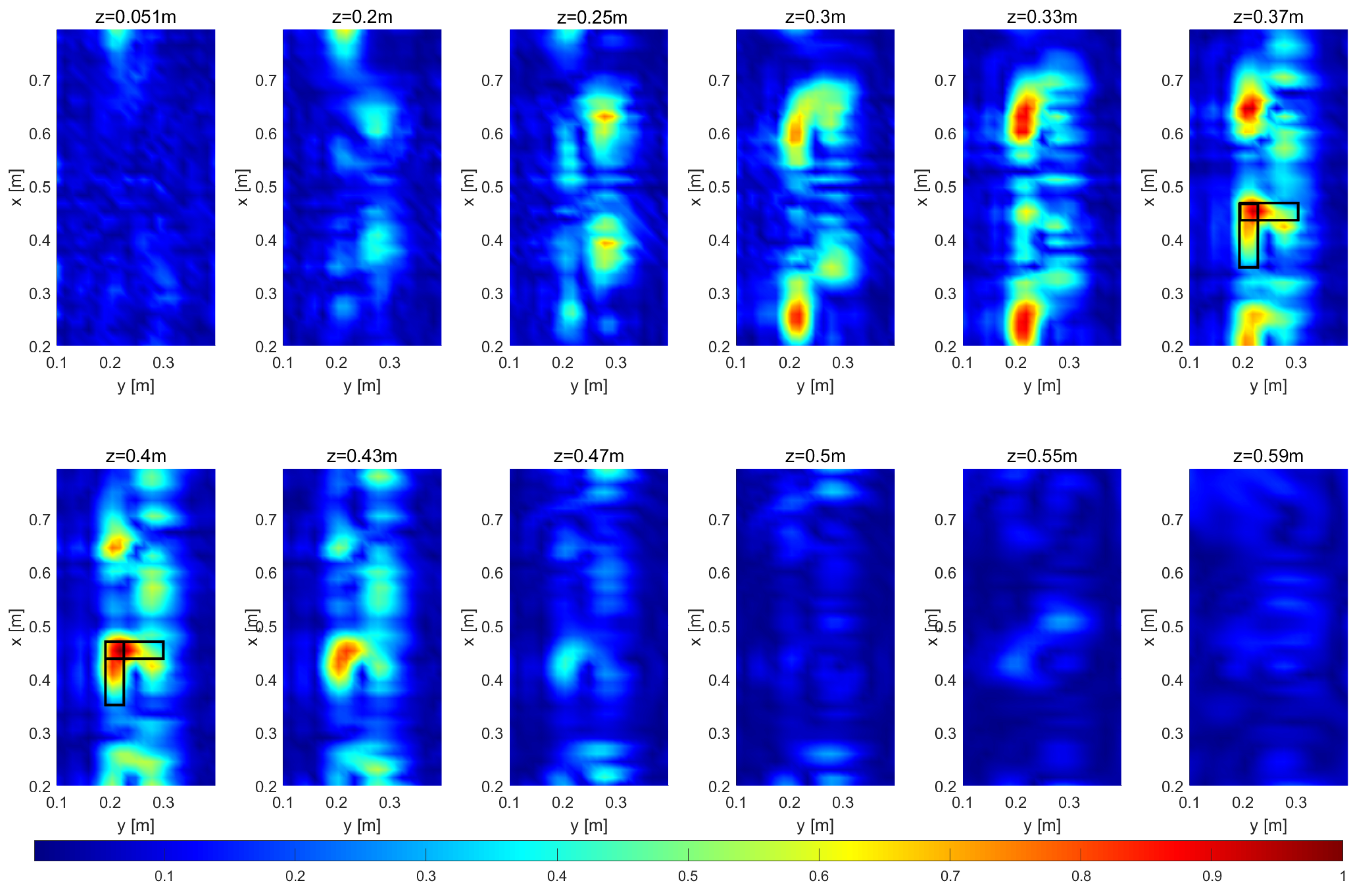
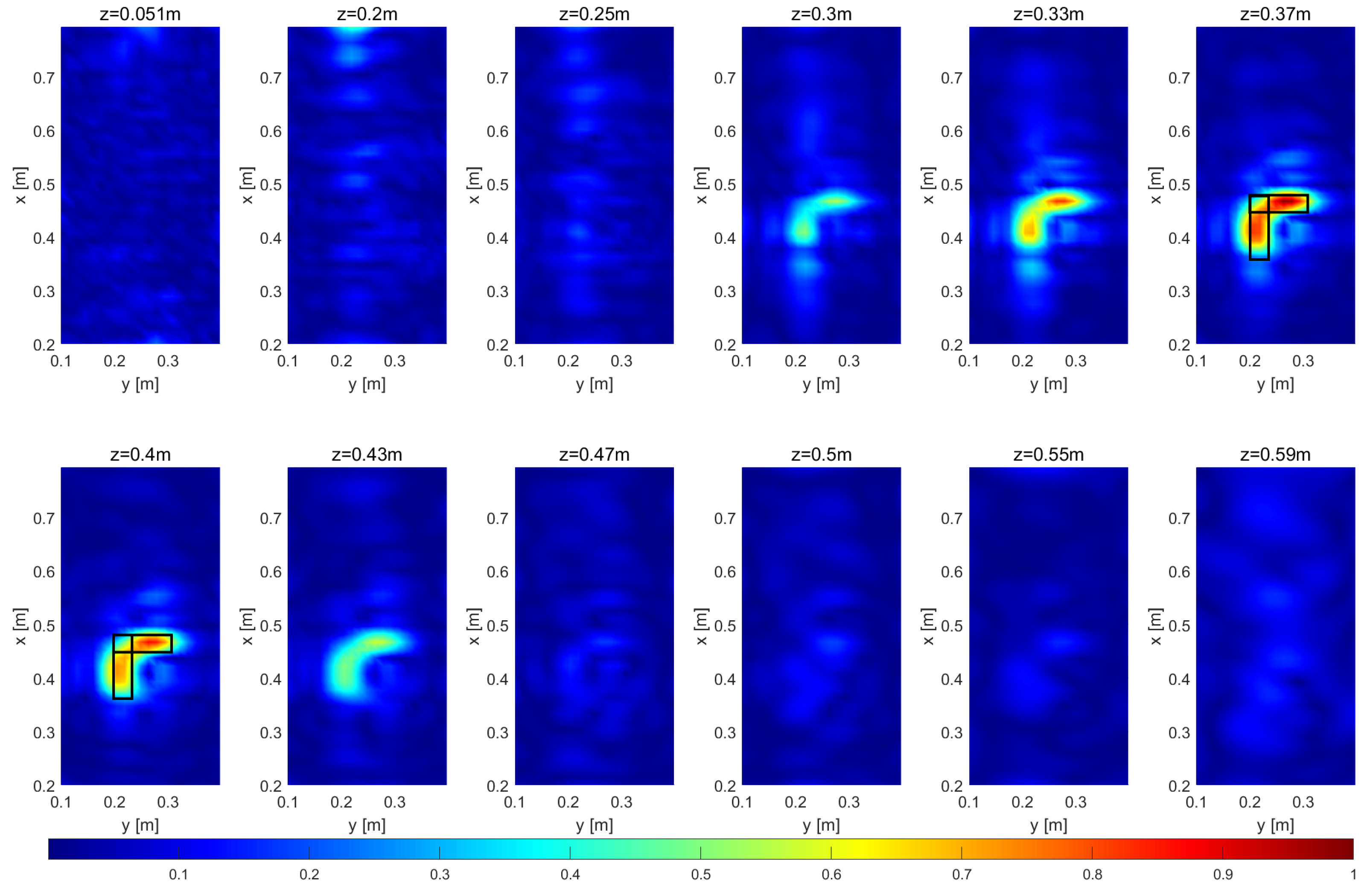
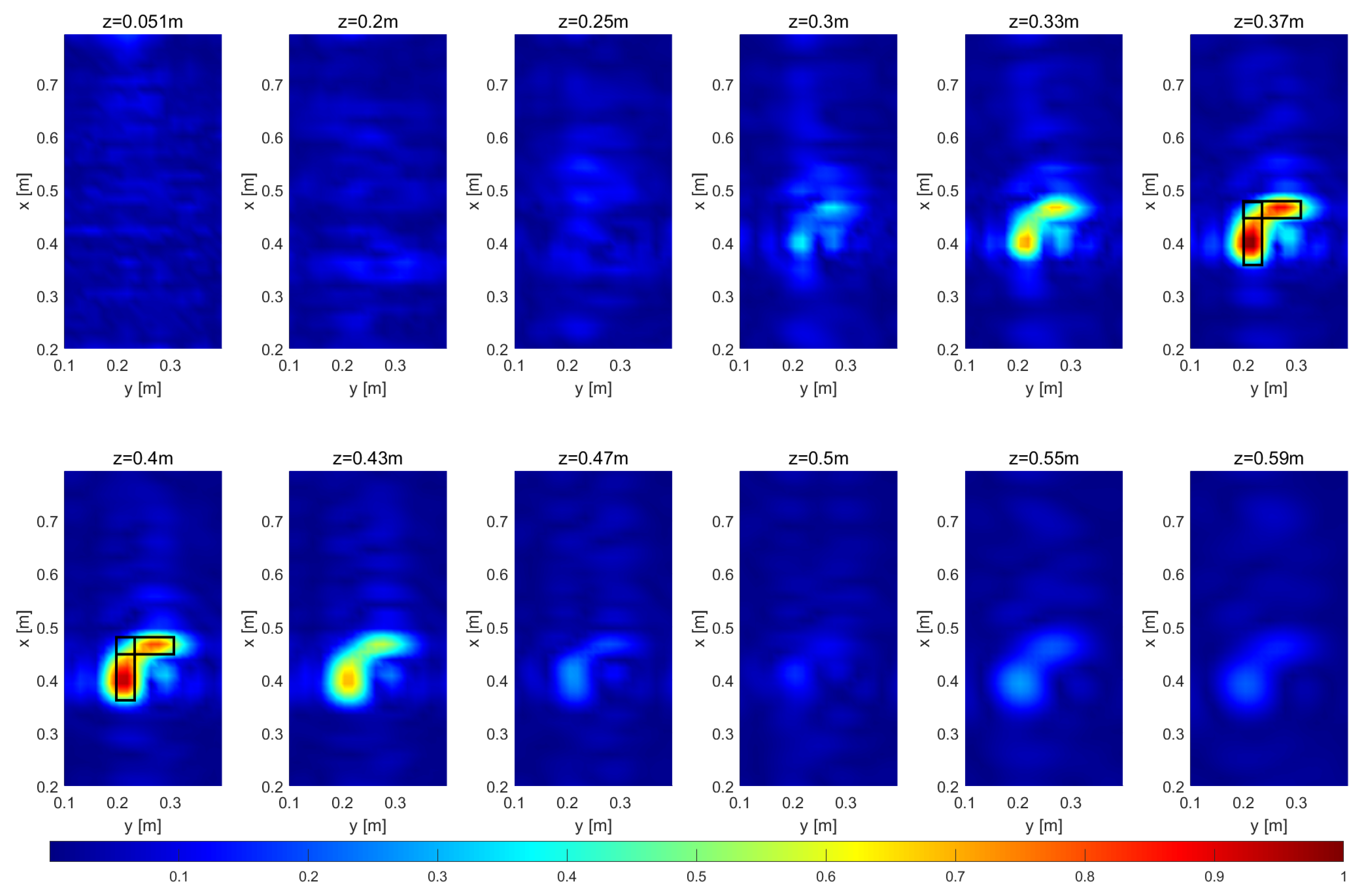
4. Reconstruction Results

This section investigates how the measurement configuration impacts the imaging capabilities in the case of extended targets. To perform this task, full-wave synthetic data are generated by using the electromagnetic simulator GPRMax [49]. In the simulated scenario, the GPR antenna array is in air and made up of x-oriented Hertzian dipoles emitting a Ricker pulse centered at the frequency of 2 GHz. As in Section 3, the GPR antennas are $7.5$ cm evenly spaced, act as Tx and Rx, and are moved with a spatial offset of 2 cm along the y-axis. The soil permittivity is ${\epsilon }_s=4$ and the investigation domain has size $[0.2,0.8]\times [0.1,0.4]\times [0,0.6]$ m³. We consider a buried L-shaped cavity (${\epsilon }_t=1$) whose position and dimensions in the $x-y$ plane are shown in Figure 8, while its thickness along z is equal to $0.03$ m. The target upper surface is located $0.37$ m below the air–soil interface. The antennas are placed at a height of 2 cm above the air–soil interface, which is small enough in terms of wavelength to neglect the propagation in air and assume a homogeneous scenario.

GPR raw data (radargrams) are generated over a fast-time window of 20 ns and processed according to the pipeline depicted in Figure 9. Specifically, the raw data are pre-processed in the time domain by means of the zero time and the time gating procedures. Firstly, a zero time setting is applied at $0.8$ ns to establish the reference point for the depth. Subsequently, the time gating is implemented by setting to zero the signal reflections up to $3.0$ ns. This gating procedure effectively eliminates artifacts arising from direct coupling between the $Tx$ and $Rx$ antennas, as well as reflections from the air–soil interface. A time window of 15 ns is considered for further processing. Following pre-processing, time domain data are transformed into the frequency domain using the Fast Fourier Transform (FFT) over the band $[1.6,2.2]$ GHz, with a step of 68 MHz. At this point, to simulate the real measurement process and assess the robustness of the imaging approach under realistic conditions, the data are corrupted by AWGN with $SNR=15$ dB.

The frequency domain data are the input of the MWT imaging approach, which provides a qualitative 3D reconstruction of the scenario under test, referred to as tomographic image. As performed for the resolution analysis, the TSVD truncation index $N_{\delta }$ is determined by the L-curve method.

The constant-depth slices of the 3D tomographic reconstruction normalized to the maximum into the investigation volume are plotted for each configuration in Figure 10, Figure 11, Figure 12 and Figure 13.

These figures corroborate that the MM/MF data do not allow a satisfactory target reconstruction because various artifacts appear in the horizontal plane along the x-axis due to the antenna spacing that is nearly equal to one wavelength in the soil at the center frequency.

On the other hand, Figure 11, Figure 12 and Figure 13 confirm that the availability of multiview-multistatic, multifrequency data allows the identification of the target’s position and shape. Indeed, the reconstructions peak at $z=0.37$ m, which corresponds to the upper target surface. However, the result referring to Case 1, i.e., when only two transmitters are employed, exhibits a slightly inferior depth resolution compared to Cases 2 and 3, although it still maintains an acceptable reconstruction quality. Conversely, all the considered multiview, multistatic, multifrequency reconstructions achieve nearly identical transverse resolution along the x- and y-axes. Notably, in agreement with the analysis in Section 3, the multiview-multistatic configuration denoted as Case 3, although its increased number of transmitters, provides a similar imaging performance to Case 2, which uses the half number of transmitters.

5. Conclusions

This paper investigated the advantages offered by MIMO GPR systems in terms of imaging reconstruction capabilities, starting from the observation that multichannel GPR systems currently available on the market not only allow the simultaneous collection of multimonostatic data along more parallel traces but also make possible the acquisition of multiview-multistatic data. Specifically, a theoretical study aimed at assessing how the availability of multiview, multistatic, and multifrequency data impact on the 3D GPR imaging, when it is faced using a microwave tomographic (MWT) approach, has been presented. The adopted MWT approach models the GPR antennas as linearly polarized electric dipoles; it faces the imaging as an inverse scattering problem by using the Born Approximation and the far-field one to describe the scattering phenomenon, and it can process both multimonostatic, multifrequency data and multiview, multistatic, multifrequency data collected by MIMO GPR systems equipped with M transmitting and N receiving antennas, with M and N arbitrary integer numbers.

The imaging capabilities of the MWT approach have been investigated by taking into account the spectral content and the point spread function as well as by processing synthetic data referring to an extended target.

The performed analysis has corroborated that the exploitation of multiview, multistatic, multifrequency data mitigates the occurrence of artifacts due to an unsuitable spacing among the antennas of the GPR arrays. Furthermore, the use of a number of Tx antennas equal to half of the total number of available antennas appears as a suitable choice for improving imaging performance by taking into account the increased measurement time required by the acquisition of multiview-multistatic data.

It is worth remarking that the presented analysis can be exploited to foresee the expected imaging capabilities in real scenarios, and future activities will regard the collection and the processing of multiview, multistatic, multifrequency experimental data to assess the achievable performances in realistic scenarios. Furthermore, since the adopted MWT approach provides a qualitative reconstruction, i.e, it provides information on the geometrical features of the targets but not on their electromagnetic properties, future research will tackle the design and validation of approaches devoted to exploiting multiview, multistatic, multifrequency data to perform the quantitative imaging of the investigated scenarios.

References

1. Daniels, D.J. Ground Penetrating Radar; John Wiley and Sons: Hoboken, NJ, USA, 2005. [Google Scholar]
2. Persico, R. Introduction to Ground Penetrating Radar: Inverse Scattering and Data Processing; Wiley: Hoboken, NJ, USA, 2014. [Google Scholar]
3. Benedetto, A.; Pajewsky, L. Civil Engineering Applications of Ground Penetrating Radar; Springer: Cham, Switzerland, 2015; ISBN 978-3-319-04813-0. [Google Scholar]
4. Catapano, I.; Crocco, L.; Di Napoli, R.; Soldovieri, F.; Brancaccio, A.; Pes, O.F.; Aiello, A. Microwave tomography enhanced GPR surveys in Centaur’s Domus—Regio vI of Pompeii. J. Geophys. Eng. 2012, 9, S92–S99. [Google Scholar] [CrossRef]
5. Soldovieri, F.; Brancaccio, A.; Prisco, G.; Leone, G.; Pierri, R. A Kirchhoff-based shape reconstruction algorithm for the multimonostatic configuration: The realistic case of buried pipes. IEEE Trans. Geosci. Remote Sens. 2008, 46, 3031–3038. [Google Scholar] [CrossRef]
6. Soliman, M.; Wu, Z. Buried object location based on frequency domain UWB measurements. J. Geophys. Eng. 2008, 5, 221–231. [Google Scholar] [CrossRef]
7. Urbini, S.; Cafarella, L.; Marchetti, M.; Chiarucci, P. Fast geophysical prospecting applied to archaeology: Results at villa ai Cavallacci (Albano Laziale, Rome) site. Ann. Geophys. 2007, 50, 291–299. [Google Scholar] [CrossRef]
8. Sato, M. MIMO Radar. In MIMO Communications—Fundamental Theory, Propagation Channels, and Antenna Systems; IntechOpen: London, UK, 2023. [Google Scholar] [CrossRef]
9. Zhang, W.; Hoorfar, A. MIMO Ground Penetrating Radar Imaging through Multilayered Subsurface Using Total Variation Minimization. IEEE Trans. Geosci. Remote Sens. 2019, 57, 2107–2115. [Google Scholar] [CrossRef]
10. Catapano, I.; Gennarelli, G.; Esposito, G.; Ludeno, G.; Su, Y.; Zhang, Z.; Soldovieri, F. Contactless Microwave Tomography via MIMO GPR. IEEE Geosci. Remote Sens. Lett. 2023, 20, 1–5. [Google Scholar] [CrossRef]
11. Zheng, W.; Hao, T.; Li, X.; Luo, W. Experimental validation of the horizontal resolution improvement by ultra-wideband metasurfaces for GPR systems. NDT E Int. 2024, 147, 103179. [Google Scholar] [CrossRef]
12. Jin, T.; Lou, J.; Zhou, Z. Extraction of Landmine Features Using a Forward-Looking Ground-Penetrating Radar with MIMO Array. IEEE Trans. Geosci. Remote Sens. 2012, 50, 4135–4144. [Google Scholar] [CrossRef]
13. Dogaru, T.; Carin, L. Time-domain sensing of targets buried under a rough air-ground interface. IEEE Trans. Antennas Propag. 1998, 46, 360–372. [Google Scholar] [CrossRef]
14. Soldovieri, F.; Gennarelli, G.; Catapano, I.; Liao, D.; Dogaru, T. Forward-Looking Radar Imaging: A Comparison of Two Data Processing Strategies. IEEE J. Sel. Top. Appl. Earth Obs. Remote Sens. 2017, 10, 562–571. [Google Scholar] [CrossRef]
15. Barbin, Y.; Nicollin, F.; Kofman, W.; Zolotarev, V.; Glotov, V. Mars 96 GPR program. J. Appl. Geophys. 1995, 33, 27–37. [Google Scholar] [CrossRef]
16. Hamran, S.E.; Paige, D.A.; Amundsen, H.E.F.; Berger, T.; Brovoll, S.; Carter, L.; Damsgård, L.; Dypvik, H.; Eide, J.; Eide, S.; et al. Radar imager for Mars’ subsurface experiment—RIMFAX. Space Sci. Rev. 2020, 216, 1–39. [Google Scholar] [CrossRef]
17. Jing, L.; Chen, Y.; Zeng, Z. Estimated lunar regolith structure based on the least-squares Kirchhoff migration of CE-3 lunar penetrating radar data. IEEE Geosci. Remote. Sens. Lett. 2020, 18, 816–820. [Google Scholar]
18. García-Fernández, M.; Álvarez-Narciandi, G.; Laviada, J.; López, Y.Á.; Las-Heras, F. Towards real-time processing for UAV-mounted GPR-SAR imaging systems. ISPRS J. Photogramm. Remote Sens. 2024, 212, 1–12. [Google Scholar] [CrossRef]
19. Catapano, I.; Crocco, L.; Isernia, T. A simple two-dimensional inversion technique for imaging homogeneous targets in stratified media. Radio Sci. 2004, 39, 1–14. [Google Scholar] [CrossRef]
20. Hajebi, M.; Tavakoli, A.; Dehmollaian, M.; Dehkhoda, P. An Iterative Modified Diffraction Tomography Method for Reconstruction of a High-Contrast Buried Object. IEEE Trans. Geosci. Remote Sens. 2018, 56, 4138–4148. [Google Scholar] [CrossRef]
21. Fischer, C.; Younis, M.; Wiesbeck, W. Multistatic GPR data acquisition and imaging. Proc. IEEE Int. Geosci. Remote Sens. Symp. 2002, 1, 328–330. [Google Scholar]
22. Counts, T.; Gurbuz, A.C.; Scott, W.R.; McClellan, J.H.; Kangwook, K. Multistatic ground-penetrating radar experiments. IEEE Trans. Geosci. Remote Sens. 2007, 45, 2544–2553. [Google Scholar] [CrossRef]
23. Nikolova, N.K. References. In Introduction to Microwave Imaging; EuMA High Frequency Technologies Series; Cambridge University Press: Cambridge, UK, 2017; pp. 327–340. [Google Scholar]
24. Pastorino, M. Microwave Imaging; John Wiley and Sons: Hoboken, NJ, USA, 2010. [Google Scholar]
25. Chew, W.C. Inverse Scattering Problems. In Waves and Fields in Inhomogenous Media; IEEE: Piscataway, NJ, USA, 1995; pp. 511–570. [Google Scholar] [CrossRef]
26. Persico, R. On the role of measurement configuration in contactless GPR data processing by means of linear inverse scattering. IEEE Trans. Geosci. Remote Sens. 2006, 54, 2062–2071. [Google Scholar] [CrossRef]
27. Noghanian, S.; Sabouni, A.; Desell, T.; Ashtari, A. Microwave Tomography; Springer: New York, NY, USA, 2014. [Google Scholar]
28. Catapano, I.; Gennarelli, G.; Ludeno, G.; Soldovieri, F.; Persico, R. Ground-Penetrating Radar: Operation Principle and Data Processing. In Wiley Encyclopedia of Electrical and Electronics Engineering; Wiley: Hoboken, NJ, USA, 2019; pp. 1–23. [Google Scholar]
29. Almeida, E.R.; Bicudo, T.; Porsani, J.L. Automatic estimation of inversion parameters for Microwave Tomography in GPR data using cooperative targets. J. Appl. Geophys. 2020, 178, 104074. [Google Scholar] [CrossRef]
30. Ambrosanio, M.; Bevacqua, M.T.; Isernia, T.; Pascazio, V. Performance Analysis of Tomographic Methods Against Experimental Contactless Multistatic Ground Penetrating Radar. IEEE J. Sel. Top. Appl. Earth Obs. Remote. Sens. 2021, 14, 1171–1183. [Google Scholar] [CrossRef]
31. Gennarelli, G.; Catapano, I.; Ludeno, G.; Noviello, C.; Papa, C.; Pica, G.; Soldovieri, F.; Alberti, G. A low frequency airborne GPR system for wide area geophysical surveys: The case study of Morocco Desert. Remote. Sens. Environ. 2019, 233, 111409. [Google Scholar] [CrossRef]
32. Soldovieri, F.; Persico, R.; Leone, G. A linear inverse scattering algorithm for the multi-monostatic GPR configuration. In Proceedings of the 3rd International Workshop on Advanced Ground Penetrating Radar, Delft, The Netherlands, 2–3 May 2005. [Google Scholar]
33. Bhat, C.; Maisto, M.A.; Khankhoje, U.K.; Solimene, R. Subsurface Radar Imaging by Optimizing Sensor Locations in Spatio-Spectral Domains. IEEE Trans. Geosci. Remote. Sens. 2023, 61, 4505310. [Google Scholar] [CrossRef]
34. Salucci, M.; Poli, L.; Massa, A. Advanced multi-frequency GPR data processing for non-linear deterministic imaging. Signal Process. 2017, 132, 306–318. [Google Scholar] [CrossRef]
35. Gennarelli, G.; Catapano, I.; Soldovieri, F.; Persico, R. On the Achievable Imaging Performance in Full 3-D Linear Inverse Scattering. IEEE Trans. Antennas Propag. 2015, 63, 1150–1155. [Google Scholar] [CrossRef]
36. Maisto, M.A.; Masoodi, M.; Pierri, R.; Solimene, R. Sensor Arrangement in Through-the Wall Radar Imaging. IEEE Open J. Antennas Propag. 2022, 3, 333–341. [Google Scholar] [CrossRef]
37. Oliveri, G.; Anselmi, N.; Massa, A. Compressive sensing imaging of non-sparse 2D scatterers by a total-variation approach within the Born approximation. IEEE Trans. Antennas Propag. 2014, 62, 5157–5170. [Google Scholar] [CrossRef]
38. Feng, X.; Sato, M. Pre-stack migration applied to GPR for landmine detection. Inverse Probl. 2004, 20, S99. [Google Scholar] [CrossRef]
39. Devaney, A.J. Geophysical diffraction tomography. IEEE Trans. Geosci. Remote Sens. 1984, 1, 3–13. [Google Scholar] [CrossRef]
40. Cui, T.J.; Chew, W.C. Diffraction tomographic algorithm for the detection of three-dimensional objects buried in a lossy half-space. IEEE Trans. Antennas Propag. 2002, 50, 42–49. [Google Scholar]
41. Bertero, M.; Boccacci, P.; De Mol, C. Introduction to Inverse Problems in Imaging, 2nd ed.; CRC Press: Boca Raton, FL, USA, 2021. [Google Scholar] [CrossRef]
42. Hansen, P.C.; Jensen, T.K.; Rodriguez, G. An adaptive pruning algorithm for the discrete L-curve criterion. J. Comput. Appl. Math. 2007, 198, 483–492. [Google Scholar] [CrossRef]
43. Castellanos, J.L.; Gómez, S.; Guerra, V. The triangle method for finding the corner of the L-curve. Appl. Numer. Math. 2002, 43, 359–373. [Google Scholar] [CrossRef]
44. Balanis, C.A. Advanced Engineering Electromagnetics; John Wiley & Sons: Hoboken, NJ, USA, 2012. [Google Scholar]
45. Hansen, P.C. Regularization tools version 4.0 for Matlab 7.3. Numer. Algorithms 2007, 46, 189–194. [Google Scholar] [CrossRef]
46. Gianluca, G.; Soldovieri, F. Radar imaging through cinderblock walls: Achievable performance by a model-corrected linear inverse scattering approach. IEEE Trans. Geosci. Remote Sens. 2014, 52, 6738–6749. [Google Scholar]
47. Gennarelli, G.; Riccio, G.; Solimene, R.; Soldovieri, F. Radar imaging through a building corner. IEEE Trans. Geosci. Remote Sens. 2014, 52, 6750–6761. [Google Scholar] [CrossRef]
48. Negishi, T.; Gennarelli, G.; Soldovieri, F.; Liu, Y.; Erricolo, D. Radio frequency tomography for nondestructive testing of pillars. IEEE Trans. Geosci. Remote Sens. 2020, 58, 3916–3926. [Google Scholar] [CrossRef]
49. Warren, C.; Giannopoulos, A.; Giannakis, I. gprMax: Open source software to simulate electromagnetic wave propagation for Ground Penetrating Radar. Comput. Phys. Commun. 2016, 209, 163–170. [Google Scholar] [CrossRef]
Figure 1. Geometry of the imaging problem.
Remotesensing 16 03163 g001
Figure 2. Two-dimensional representation of the considered geometry highlighting the maximum angular illumination.
Remotesensing 16 03163 g002
Figure 3. Antenna array configuration for the considered cases.
Remotesensing 16 03163 g003
Figure 4. Singular values of the operator A relevant to the considered measurement configurations represented over a dB scale.
Remotesensing 16 03163 g004
Figure 5. The L-Curves relevant to each configuration.
Remotesensing 16 03163 g005
Figure 6. Cuts of the normalized spectral content relevant to the considered cases. The panels in the first row (a1d1) represent the cuts in the k x k z plane, while the panels in the second row (a2d2) are the cuts in the k y k z plane.
Remotesensing 16 03163 g006
Figure 7. Comparison of the PSF cuts related to a point-like target placed at (0.5, 0.25, 0.3) m. Panels (ac) show the PSF cuts along x, y and z, respectively.
Remotesensing 16 03163 g007
Figure 8. Geometry of the simulated scenario.
Remotesensing 16 03163 g008
Figure 9. Data processing flow chart.
Remotesensing 16 03163 g009
Figure 10. Depth slices of the full-3D tomographic reconstruction of the L-shaped target referring to MM/MF configuration. Color scale [ 0 , 1 ] .
Remotesensing 16 03163 g010
Figure 11. Depth slices of the full-3D tomographic reconstruction of the L-shaped target referring to Case 1. Color scale [ 0 , 1 ] .
Remotesensing 16 03163 g011
Figure 12. Depth slices of the full-3D tomographic reconstruction of the L-shaped target referring to Case 2. Color scale [ 0 , 1 ] .
Remotesensing 16 03163 g012
Figure 13. Depth slices of the full-3D tomographic reconstruction of the L-shaped target referring to Case 3. Color scale [ 0 , 1 ] .
Remotesensing 16 03163 g013