Abstract
Global warming and climate change are significantly impacting local climates, causing more intense heat during the summer season, which poses risks to individuals with pre-existing health conditions and negatively affects overall human health. While various studies have examined the Surface Urban Heat Island (SUHI) phenomenon, these studies often focus on small to large geographic regions using low-to-moderate-resolution data, highlighting general thermal trends across large administrative areas. However, there is a growing need for methods that can detect microscale thermal patterns in environments familiar to urban residents, such as streets and alleys. The temperature-humidity index (THI), which incorporates both temperature and humidity data, serves as a critical measure of human-perceived heat. However, few studies have explored microscale THI variations within urban settings and identified potential THI hotspots at a local level where SUHI effects are pronounced. This research aims to address this gap by estimating THI at a finer resolution scale using data from multiple sensor platforms. We developed a model with the random forest algorithm to assess THI trends at a resolution of 0.5 m, utilizing various variables from different sources, including Landsat 8 land surface temperature (LST), unmanned aerial system (UAS)-derived LST, Sentinel-2 NDVI and NDMI, a wind exposure index, solar radiation modeled from aircraft and UAS-derived Digital Surface Models, and vehicle density and building floor area from social big data. Two models were constructed with different variables: Modelnatural, which includes variables related to only natural factors, and Modelmix, which includes all variables, including anthropogenic factors. The two models were compared to reveal how each source contributes to the model development and SUHI effects. The results show significant improvements, as Modelnatural had a fitting R2 = 0.5846, a root mean square error (RMSE) = 0.5936 and a mean absolute error (MAE) = 0.4294. Moreover, when anthropogenic factors were introduced, Modelmix performed even better, with R2 = 0.9638, RMSE = 0.1751, and MAE = 0.1065 (n = 923). This study contributes to the future of microscale SUHI analysis and offers important insights into urban planning and smart city development.
1. Introduction
The large concern related to surface urban heat islands (SUHIs) has been well documented in numerous remote sensing studies over the past few decades. These studies consistently demonstrate that urbanization leads to significantly higher thermal conditions in densely populated urban centers compared to surrounding suburban areas [1]. Following urbanization, the SUHI phenomenon has become prominent in various cities worldwide [2]. It induces problematic environmental issues that can cause various hazards, such as increased high-temperature nights and their associated health hazards (e.g., heat strokes), changes in ecosystems allowing mosquitoes, which carry infectious diseases, to expand their habitat, and increasing the frequency of intense rainfall events [3]. The UHI phenomenon is a severe problem that significantly affects urban space environments and leads to associated health issues [4,5,6]. For example, the United Nations projects that by 2050, 68% of the global population will live in urban areas [7], meaning that more people will surely be exposed to higher risks in the future. Devising mitigation plans for such issues is an urgent task.
Depending on the objective and the scale of observations, the UHI phenomenon can be categorized into different layers based on altitude: the boundary layer UHI, the canopy layer UHI (CUHI), the surface UHI (SUHI), and even subsurfaces [3,8,9,10]. The boundary layer UHI extends from the rooftop level upwards into the atmosphere, where it influences broader meteorological conditions. The UHI canopy layer is found within the urban canopy, which includes the space from ground level up to the average rooftop height, where most human activities occur. Lastly, the SUHI is observed directly at the land surface level and is commonly assessed using remote sensing technologies, such as satellite imagery, to measure land surface temperature (LST) trends. Traditionally, the term UHI has referred to the phenomenon where urban areas exhibit higher temperatures than their surrounding rural areas, particularly at night, due to the heat retention properties of urban infrastructure [9]. This nocturnal temperature differential has been the subject of extensive studies, providing valuable insights into the broader impacts of urbanization on local climates. However, our study specifically focuses on the daytime SUHI, primarily examining LST variations within urban areas using multiplatform remote sensing techniques. By concentrating on SUHI during daylight hours, we aim to capture the spatial heterogeneity of thermal conditions across the urban landscape, particularly in areas where the effects of SUHI are most pronounced. This approach is critical for identifying microscale thermal patterns that are essential for effective urban planning and public health interventions, as these patterns directly influence human comfort and exposure to heat during the day, when outdoor activities are most common.
Detecting LST trends through remote sensing techniques has been widely applied in various geographical regions worldwide. Estoque and Murayama [11] focused on the mountainous region and the surrounding environment in Baguio City, Philippines, through a temporal set of LANDSAT satellite series for monitoring thermal trends. The loss of green space and rapid urbanization increased the mean LST by over 3 °C above impervious surfaces from 1987 to 2015. Ranagalage et al. [12] analyzed the temporal changes in LST over the Colombo Metropolitan Area, Sri Lanka, using LANDSAT data from 1997 to 2017 and identified the critical areas that are highly exposed to thermal threats. Depending on the spatial extent and the temporal scale, the data used for analysis have mostly been derived from the LANDSAT series or MODIS satellites [13,14]. However, other options exist, such as the ASTER datasets [15] and, more recently, the ECOsystem Spaceborne Thermal Radiometer Experiment on Space Station (ECOSTRESS) LST dataset, which offers high temporal resolution [16]. While LANDSAT and MODIS are often preferred due to their widespread availability, ECOSTRESS may outperform these other spaceborne products due to its capability to capture the LST with greater frequency. Nevertheless, all the data can provide promising results in detecting the thermal condition and are valuable for observing general trends at low-to-moderate resolutions. Recent advancements in modern technology, such as unmanned aerial systems (UAS), now offer the ability to observe surface heat trends at much lower altitudes, allowing for observing the thermal distribution heterogeneity in complex urban landscapes at much finer resolutions [17,18].
The contributions to the SUHI effect can be discussed from the perspective of multiple driving factors [11,12,13,14,19,20,21,22,23,24,25]. In general, it is known that various LULC types can reduce or enhance the SUHI effect, such as impervious surfaces, which are most common in built-up urban areas, and these types of surfaces have a higher potential for surface heat storage and absorption of more solar radiation, which contributes to heating [11,19]. Conversely, vegetation, such as shrubs and trees, can reduce the heating effects through evapotranspiration [11,12,20]. The SUHI effect can also be influenced by the climate’s wet or dry conditions. For example, due to convective heat loss, dry built-up areas can act as a cooling source compared to surrounding rural lands, which tend to have wetter conditions because of vegetation [21]. Rain events and increased cloud cover diminish the overall thermal load in urban areas, temporarily alleviating SUHI intensity during daytime, particularly in warmer and wetter climates where precipitation is more frequent [13]. When investigating the phenomenon at a microscale, the shadowing effects from vertical structures, such as large buildings or trees, can directly block radiation from heating surfaces [20,22], thus working as a cooling source. Anthropogenic sources can also contribute to SUHIs, such as energy consumption [14,23] or heat emissions from buildings and vehicles [24]. Multiple factors control the SUHI, and determining how such factors are intercorrelated is often difficult. Although studies have typically relied on low-to-moderate-resolution data to capture general trends, recent research emphasizes the importance of finer-resolution analyses to detect critical microscale variations in urban environments [20,25,26].
Japan has been developing, and similar significant changes in thermal conditions are evident in urban areas (Figure 1). Due to global warming and the associated environmental issues, unusual climatic conditions have been reported [27]. Not only is the issue of heat critical, but with the geographical characteristics of Japan, which is located in a moist climatic zone, there are more chances that high temperatures can negatively impact human health. Human sensations associated with various climatic conditions can be considered using indices reflecting both temperature and humidity information. The temperature-humidity index (THI) represents the discomfort humans (or animals) feel depending on the combination of low to high temperatures and relative humidity. Temperature and humidity levels affect our health care [4,5], and extreme exposure to such high-risk conditions can even lead to death. The aging issues of the increasingly elderly population in Japan present concerns regarding the vulnerability of specific age groups to exposure to critical climatic situations [28], and it is necessary to understand where high-risk areas exist.
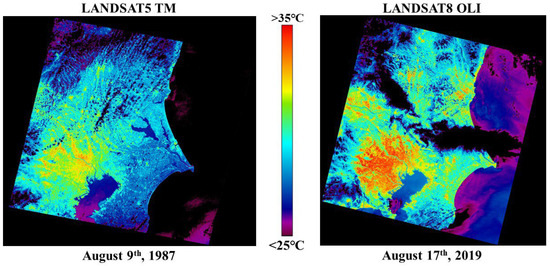
Figure 1.
Brightness temperature transition of the Tokyo metropolitan area and the surrounding landscape in Japan. Urban areas feature high temperatures, and the surrounding regions exhibit increasing thermal trends because of urban development.
Therefore, determining high-temperature hotspots and the distribution of high-discomfort (high-THI) areas in urban areas has become an issue. Numerous examinations have been conducted on the heat in metropolitan spaces [29]. Nonetheless, the outcomes are arranged to determine the pattern for an entire city or area. Such work appraises the heat trends over a moderately large administrative unit [13,30]. However, microscale studies have demonstrated the significant impact of urban geometry on microclimatic conditions. For instance, diverse urban forms and heterogeneous building heights can generate more favorable microclimate conditions, creating shaded areas, and promoting better ventilation [31]. Similarly, it is highlighted that the sky view factor (SKV) correlates to thermal comfort, which varies in seasons, where areas with higher SVF are warmer and less comfortable in the summer, while areas with high SVF in the winter tend to show higher comfort (at F26<PET<30 condition) [32]. It implies the importance of incorporating complex urban geometries into city planning to optimize outdoor thermal environments [31,32]. These findings reinforce the need to analyze urban environments at a finer scale, including specific buildings, streets, and roads, to develop targeted interventions that can effectively mitigate the adverse effects of SUHIs. However, it is equally important to maintain a broader spatial perspective that encompasses the entire city to understand how these localized conditions fit into the larger urban landscape. Achieving this balance is essential for comprehensive urban climate assessments, especially when considering the variability of conditions across different urban areas. To this end, employing cost-effective, remotely sensed approaches allows for efficient monitoring and analysis of microscale and macroscale thermal environments, providing a geographical overview critical for informed urban planning and decision-making.
In this work, our objective is to develop a new method for observing and mapping discomforts (i.e., THI) at the microscale while maintaining a broad spatial extent representing the urban landscape. The THI is chosen for its practicality, simplicity, and compatibility with available data sources. The novel contribution of this work is twofold. First, multiplatform data are processed and modeled to develop a microscale estimate of the THI distribution. The second involves determining how different driving factors contribute to the model’s accuracy by categorizing them into two major types: natural factors and anthropogenic factors. Satellite and aircraft images are collected and processed as broad-scale datasets, while an UAS is utilized to collect finer-resolution data in-situ. Two multiresolution datasets are combined with the in situ ground truth data to enhance the model estimation performance.
2. Equipment and Datasets
2.1. Unmanned Aerial System (UAS) and Camera Specification
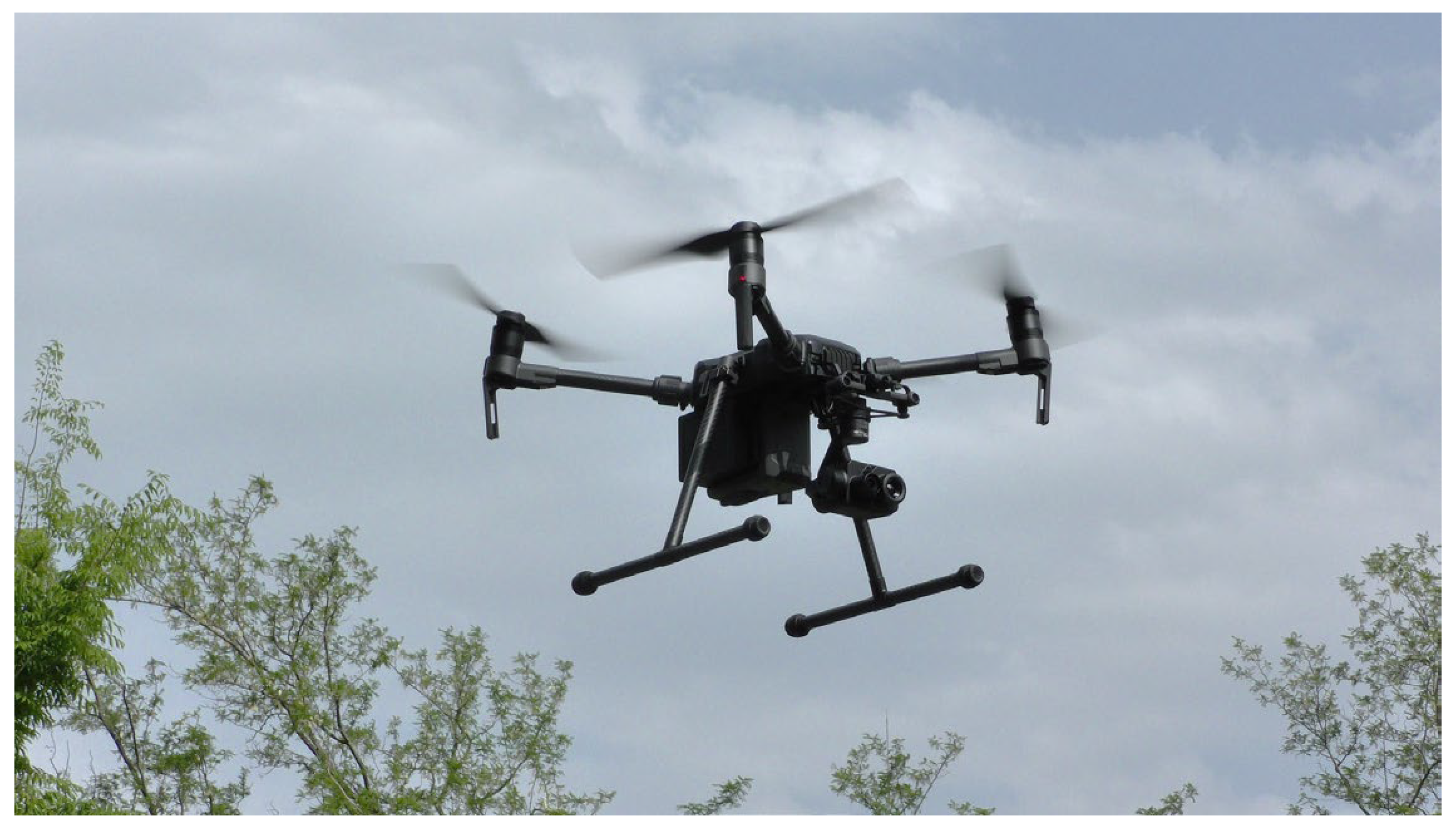
A UAS is utilized to collect finer-resolution remote sensing data at a test site (Figure 2). This work utilizes a DJI Matrice 210 multicopter UAS (DJI, Shenzhen, China) for the aerial system, and the DJI Zenmuse-XT2 (DJI, Shenzhen, China) is the sensor that is equipped aboard the UAS. The extensibility of the Matrice 210 is suitable for replacing various sensors for the objective of the flight. In this case, the Zenmuse-XT2 can capture both optical and thermal information at once, making it convenient for obtaining the data. The dual battery system enhances the flight performance for its flight duration and safety features, which makes it much safer to operate in urban areas.
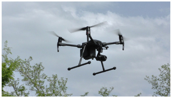
Figure 2.
The UAS utilized in this work (Matrice 210 and Zenmuse-XT2).
2.2. GNSS and Thermohygrometer
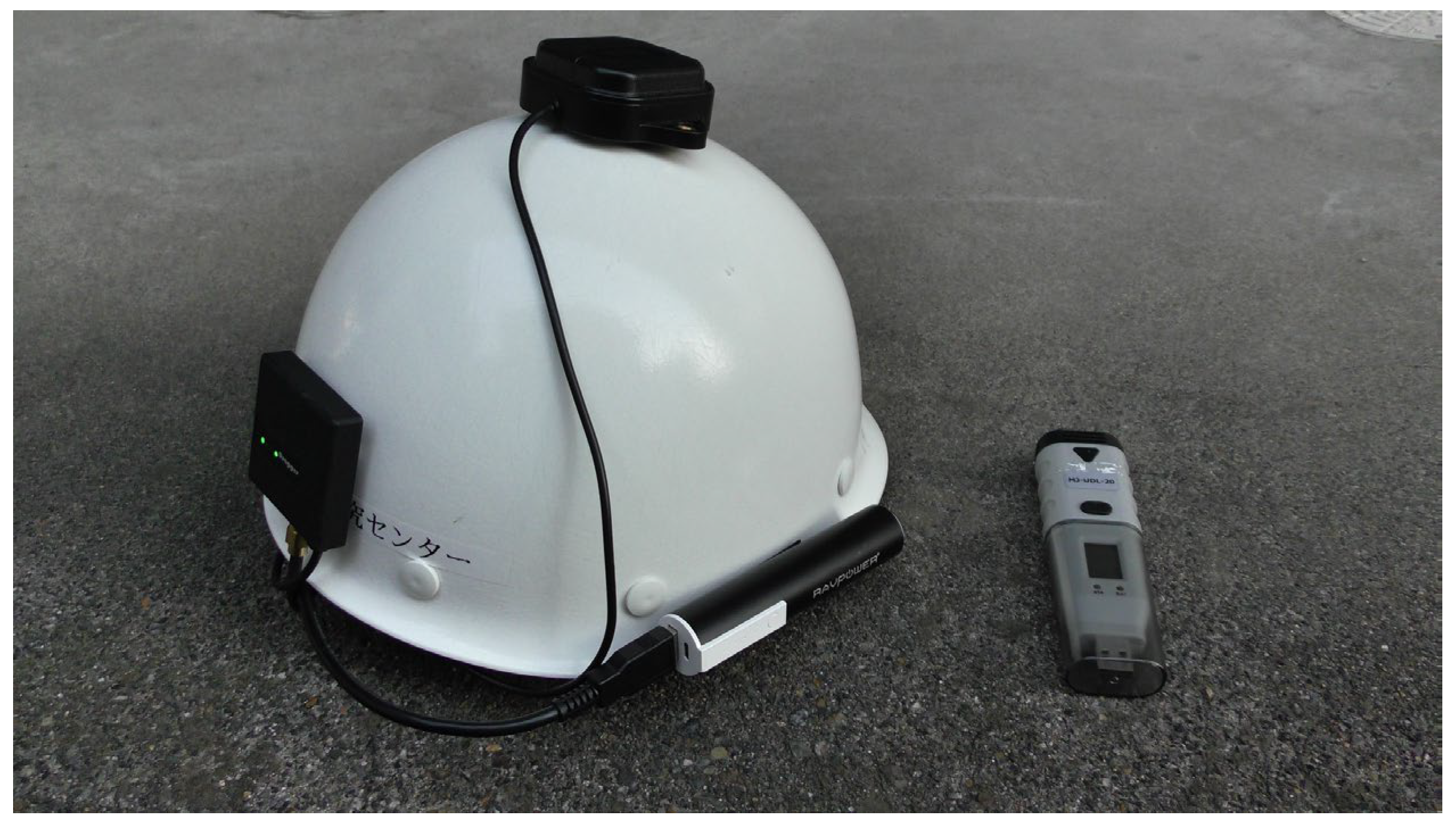
Reach (Emlid, Hong Kong) and DG-PRO1RWS F9P (BizStation Corp., Matsumoto, Japan) global navigation satellite system (GNSS) devices were utilized to record the geographical coordinates (Figure 3). The devices can record multiple L1 GNSS signals, e.g., GPS (Global Positioning System), QZSS (Quasi-Zenith Satellite System), GLONASS (Global Navigation Satellite System), Galileo, BeiDou, etc., for the Reach and both L1 and L2 signals for the F9P device (dual-frequency GNSS). The equipment was used together with a thermohygrometer to record the temperature and relative humidity at each geographical location. The two GNSS devices were used in different situations: the Reach device was utilized more in open areas, while the F9P device was used in densely built-up areas, where the limited sky view can impact the GNSS signals. An MJ-UDL-20 thermohygrometer logger (SATOTECH, Kawasaki, Japan) was used for logging the temperature and humidity with a minimum interval of 2 s. The temperature and humidity measurement ranges are −20 to 70 °C and 5 to 95%, respectively. The temperature resolution is 0.1 °C, and the relative humidity (RH) resolution is 0.1%. The sensor accuracy is ±0.5 °C (within the range of 10–60 °C) and ±3.0% for RH (within the range of 20–80% RH). The instrument has been calibrated. However, it is not ventilated and does not include a conventional radiation shield. The data is further utilized as the ground truth information of the area.
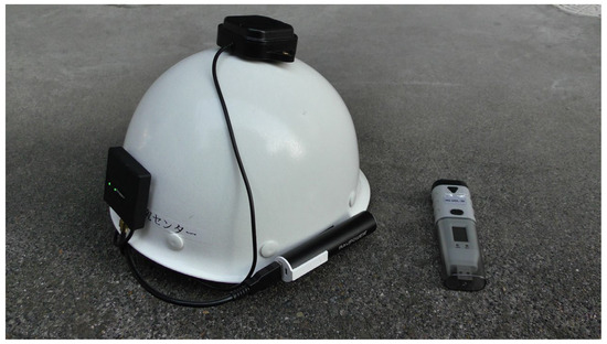
Figure 3.
GNSS equipment (F9P) attached to a helmet (left) and a thermohygrometer (right).
2.3. Satellite and Aircraft Data
Two different satellites are utilized for each purpose. First, the Sentinel-2A Mul-tispectral Instrument (MSI) Level 2A (L2A) product collected on 20 August 2020, was obtained from the relevant webpage. The L2A product is atmospherically corrected and in a ready-to-use form converted into the surface reflectance (bottom of atmosphere reflectance). The original resolution of the data is 10 m, and Sentinel data are further used for the modeling. Second, the Landsat 8 Operational Land Imager (OLI) and Thermal Infrared Sensor (TIRS) Level 1 terrain-corrected product (L1TP) collected on 26 August 2020, was obtained from the relevant webpage. The product is radiometrically corrected using the cosine of the solar zenith angle correction (COST) model [33] for conversion into surface reflectance. The data are further used for city-scale analysis. Both satellite data were cloud-free for the range of the study area. Aircraft data were collected with the support of Maebashi City Hall. The aerial survey was conducted on 10 November 2019, observing all of Maebashi city (our study area). The data are utilized to develop a 3D model of the city, and the original image resolution is approximately 16 cm.
2.4. Flight Design for UAS
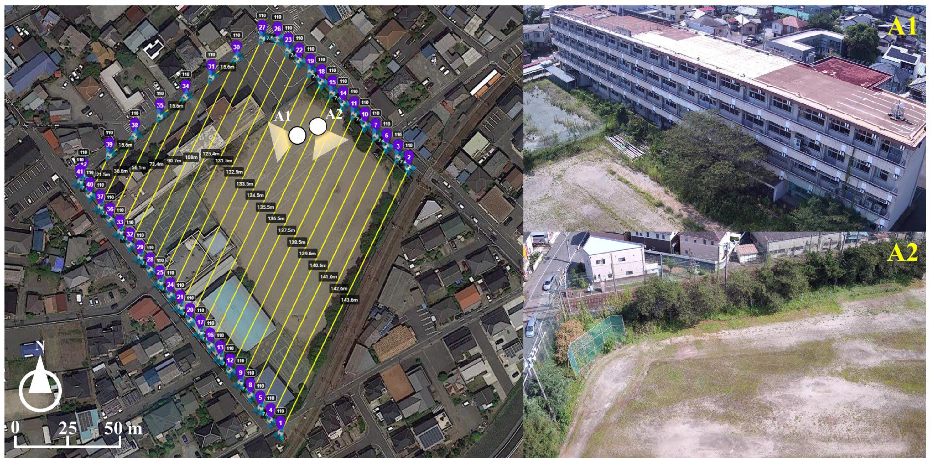
On 25 August 2020, a flight campaign was conducted at a small study site (Figure 4) from 11:00 AM to 11:10 AM. Due to an issue with a local resident, the flight was delayed by one hour. An overview of the geographical location is shown in Figure 5. The UAS operated at an altitude of 110 m following a single grid pattern (Figure 4), capturing multiple aerial photographs. The ground sampling distance (GSD) at this altitude was approximately 2.6 cm for the visible sensor and 10 cm for the thermal sensor. The forward (side) overlap for the thermal camera was set to about 84% (90%), which corresponds to roughly 89% (>90%) for the visible sensor. This survey aimed to collect microscale data samples.

Figure 4.
The flight path of the UAS for site 1 and the aerial views of the area. A1 is the main building of the closed junior high school. A2 is the school ground with partial vegetations covering.
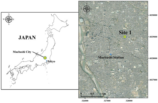
Figure 5.
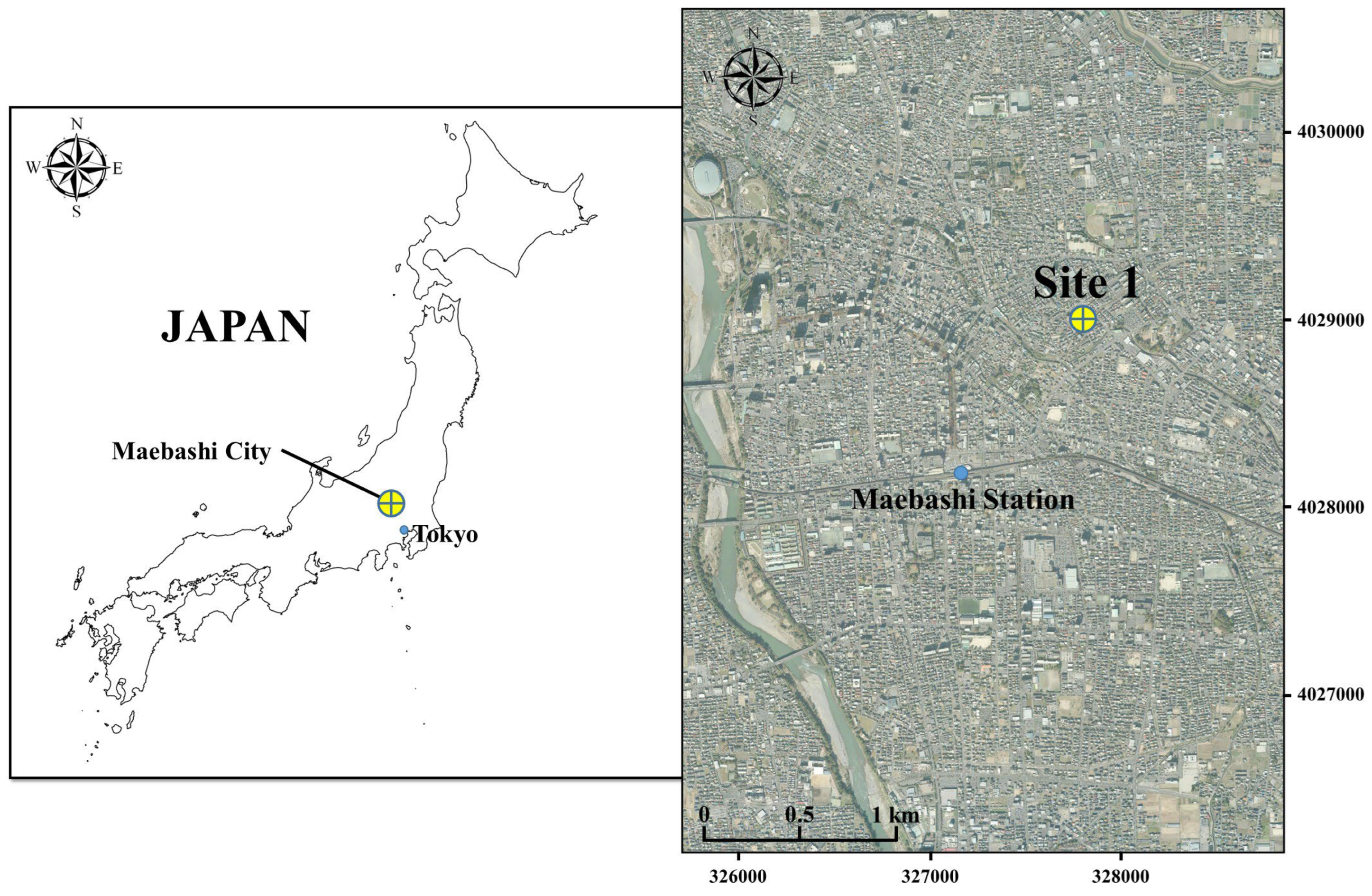
Overview of the study area (Gunma Prefecture, Maebashi City, Japan). Site 1 refers to the UAS survey site, while the whole scene shown on the right indicates the study region of the broad-scale estimation.
2.5. Ground Truth Collection of the Reference THI
2.5.1. Ground Truth at Site 1
A GNSS device (Reach or F9P) was mounted on top of a safety helmet, with a GNSS base station on a nearby tripod. The thermohygrometer was fixed to the end of a rod, held horizontally with the sensor oriented perpendicularly to the ground, and maintained at 1.3 m above ground using a string. During the UAS aerial survey, three crew members, equipped with helmets and thermohygrometer rods, walked around the study site to log geographical position, temperature, and humidity. The GNSS devices observed signals from GPS, QZSS, Galileo, and Beidou at a 1 Hz logging frequency, while the thermohygrometer recorded data every 2 s. GNSS signal data from the base station were combined with rover data for postprocessing kinematic (PPK) analysis [34] to enhance positioning accuracy (only the Reach module required postprocessing, as the F9P was sufficiently accurate without it). The GNSS and thermohygrometer timestamps were synchronized to create point vector data for temperature and humidity at each location [22]. Using Equation (1) [35], the THI was calculated for each point, representing the level of discomfort due to temperature and humidity. According to Yoo and Chung [35], a THI below 68 indicates comfort, 68–75 represents initial discomfort, 75–80 causes discomfort for 50% of people, and above 80 results in distress for all individuals.
where T is the temperature (°C), and RH is the relative humidity (%).
2.5.2. Ground Truth Within the City
On 26 August 2020, the same procedure as site 1 was performed within multiple areas of the city. From 10:00 AM to 10:30 AM, five crews walked across the city to collect temperature and humidity data. Each crew was set to different starting locations from a posteriori knowledge: a park (area with grass, shrub, and tree vegetation), an open built-up area, a central station and the surroundings, residential houses, and the city’s main tree-lined street with trees that cast shadows (Figure 6). Multiple areas were selected to provide various types of samples. The date and the time of the ground truthing coincided with the Landsat observations, which were observed on the same day at approximately 10:20 A.M. local time. The sample points were converted to point vectors, and THI values were computed as indicated in Section 2.5.1. Figure 6 shows the overview of the sampled area and images of each location. Any samples collected at a location where the sky was not visible were excluded from the analysis.
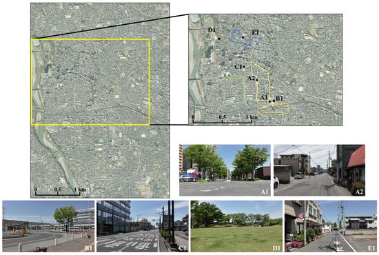
Figure 6.
The geographical location of the sampled areas for ground truth and the images from each location. A1: city’s main tree-lined street, A2: residential houses, B1: central station and the surroundings, C1: open built-up area, D1: park, E1: residential houses.
2.6. Mobility and Building Floor Data
Mobility big data was collected from Agoop Corp. (Tokyo, Japan). The data is structured in CSV format, containing unique IDs, coordinates, and logging times, which allows for the analysis of mobility flow dynamics. To consider the anthropogenic effects, the mobility information of Maebashi City was extracted for 7 August 2019. The date did not coincide with the actual ground-truthing date; however, it was used considering the same day of the week and climate conditions (clear day). The period of the field study did not coincide with any lockdowns amidst COVID-19; therefore, it is assumed that a significant traffic difference will not be seen. The building floor data were created using the digital residential map of Zenrin Co., Ltd. (Kitakyushu, Japan). The residential map is a large-scale map and covers almost all of Japan. Using this map, it is possible to evaluate the location, shape, and number of floors of buildings. The building information on this map is very reliable because it was created based on topographical maps and basic city planning maps produced by the Geospatial Information Authority of Japan, and the results of field surveys of all buildings are reflected in the map. Similar large-scale maps have been developed in the United States, France, South Korea, and other countries, and in the United Kingdom, as in Japan, large-scale maps have been published by private companies (UKMap by G.I.group (Chesterfield, United Kingdom) [36]. In this study, we used the digital data from this map created in 2019 to collect the total floor area of all buildings in the target area.
3. Methodology
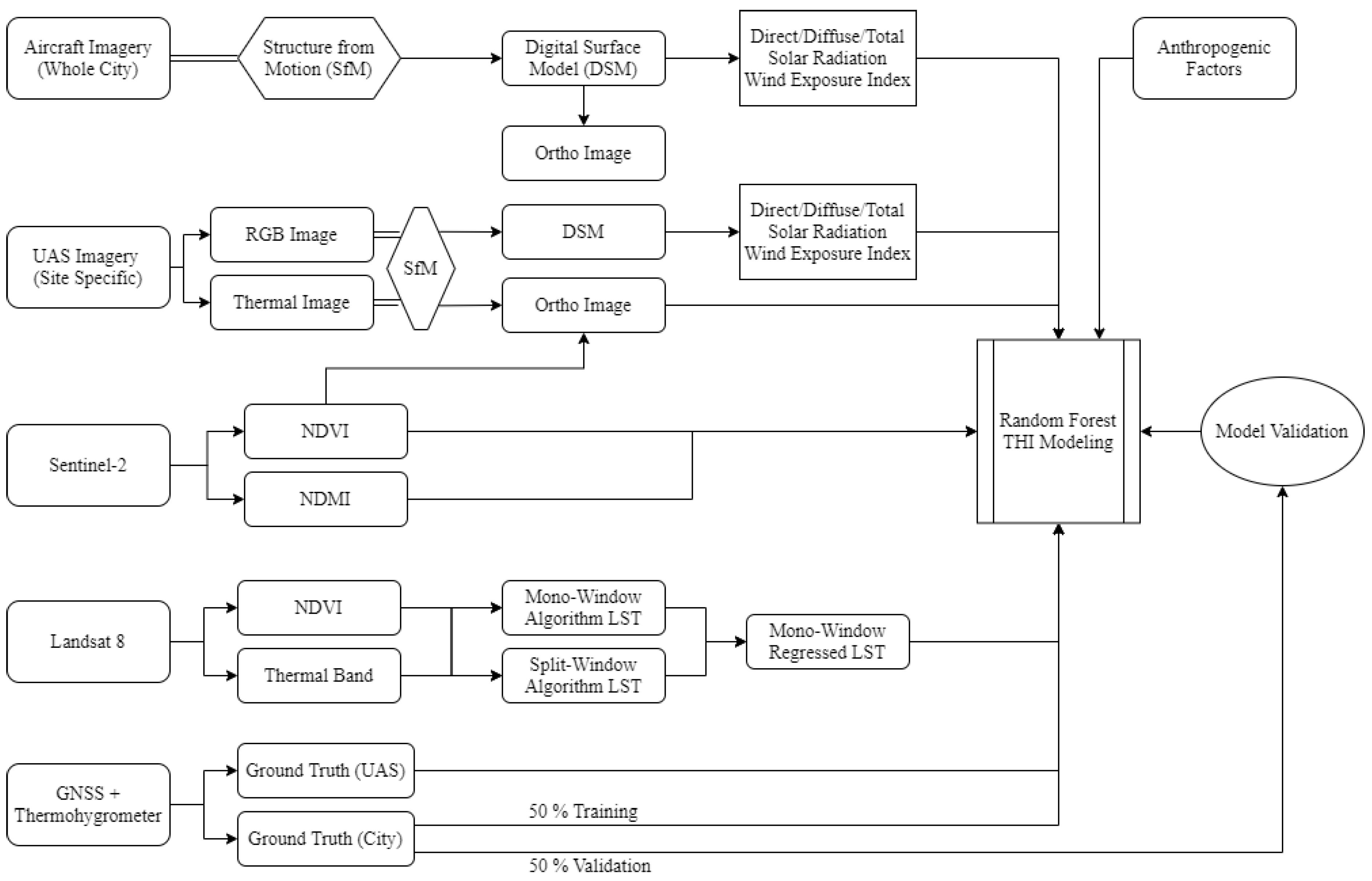
The data introduced in this study include multiple types and are in the form of large datasets. We have summarized the methodological flow of this work process in Figure 7. The objective of this work is to map the distribution of the THI and analyze thermal heterogeneity within SUHI-affected areas at a microscale resolution. Aircraft and satellite data are used, which can cover larger spatial extents; however, UAS data are also included to improve model accuracy. This is from the assumption in works by Iizuka et al. [37], which discusses that model improvements can be achieved by integrating finer-resolution information with coarser-resolution information. Aircraft data are used to develop a 3D model of the whole scene. Satellite data are used to compute the LST for the scene or compute the emissivity in order to adjust the UAS data. The GNSS and thermohygrometer devices are utilized to collect the ground-truth THI values used as training data for model development. Note that all the UAS sample data points are used for model development, while the ground-truth data collected within the city is divided in half, creating a training set and a validation set. Finally, with multiple variables, the random forest model is trained, and two models are computed: Modelnatural, in which only variables related to natural factors are used, and Modelmix, in which anthropogenic factors are included.

Figure 7.
Overall flowchart of the methods. The main datasets are listed on the far left and each process and usage of each data is shown through the flow. An additional variable is included in the final modeling process and two different models are output: variables containing only natural factors and both natural and anthropogenic factors.
3.1. Study Area
The study area, Maebashi City, Gunma Prefecture, is located in the northwestern area of the Tokyo metropolitan region in Japan and is centered on the island, with the greatest possible distance to the east and west coasts (Figure 5). The study area for the whole city scale is focused on the central area of the city, where the main Maebashi station is located in the scene center (densely urbanized area). To the south and north-east, there are sparser built-up areas, and patches of agricultural land start to appear. The western side features a river crossing from north to south through the city. The site length in the north-south direction is approximately 4.5 km, and that in the east-west direction is approximately 3.2 km. Site 1 in the figure indicates the area where the UAS survey was conducted. Site 1 is a closed junior high school with variations in land cover, including bare soil, grassy vegetation, trees, buildings, and asphalt, each exhibiting different thermal trends. Microscale sampling was conducted in this area. The climatic conditions of Maebashi city vary within a year. Our fieldwork was carried out on 25–26 August 2020. The daily average maximum temperature in August 2020 was 35.1 °C, and the peak maximum reached 39.8 °C. Maebashi City is always given attention to the nation’s temperature observations because this region is characterized by a hot summer climate. The total precipitation was 64.5 mm, and the average relative humidity was 68%, which indicates extremely hot and moist conditions, leading to much higher discomfort.
3.2. Spatial Data and Variable Construction
3.2.1. Aerial Image and Digital Surface Model
Using the collected aircraft and UAS optical and thermal imagery, the structure from motion (SfM) technique was applied with Metashape Pro ver. 1.6.0. (Agisoft, St. Petersburg, Russia) for creating an ortho imagery. Specific parameter settings for the optical image are follow: alignment = “high”, default ties and key points, dense point = “ultrahigh”, depth filtering = “mild”. Digital surface model (DSM) is generated with a dense point cloud, further used for orthorectifying the images. The DSM was generated using the inverse distance weighting (IDW) interpolation algorithm. Thermal image uses the follow: alignment = “highest”, default ties and key points, dense cloud = “ultrahigh”. Instead of a DSM, mesh data were created to produce a mosaicked thermal image. The original resolution of the processed aircraft data for the DSM and orthoimage was approximately 15 cm, resampled to 0.5 m using the bilinear method for further processing. The UAS data had resolutions of 5 cm for RGB and 10 cm for thermal data, with the RGB data (DSM) resampled to 10 cm using the bilinear method to match the thermal data.
3.2.2. Solar Radiation and Wind Exposure
The accumulated total, direct, and diffuse shortwave solar radiation were modeled using the DSM, with ArcGIS Pro ver. 2.4. (ESRI, Redlands, CA, USA) for the same date and time as the observations. For site 1, solar radiation was modeled from sunrise to 11:00 AM, while the entire city was modeled from sunrise until 10:30 AM every 0.5 h. The System for Automated Geoscientific Analyses (SAGA) GIS [38] ver. 7.7.1. is used to generate a wind exposure index [39] to determine the degree of exposed areas. The search radius is set to 20 m. Depending on the location and surrounding objects, there are different degrees of wind, which will influence the neighborhood heat exchange related to evaporation [40]. Modeling the magnitude of wind effects should work as an alternative to the actual wind velocity, which would be complex to obtain for each area.
3.2.3. Satellite Indices
Landsat 8 data are utilized to compute the LST for the city. This approach proposes both the mono-window algorithm (MWA) and split-window algorithm (SWA) integration. MWA and SWA is guided by the work of Wang et al. [41]. The improved MWA for the band 10 Landsat 8 data can be computed from the following equation [41]:
where TMW is the LST from the MWA method and a10 and b10 are constants (for this study: a10 = −70.1775, b10 = 0.4581). C10 and D10 are emissivity functions (ε10) and atmospheric transmittance (τ10). T10 is the brightness temperature of band 10. Ta is the effective mean atmospheric temperature. C10 and D10 are calculated by:
Estimating emissivity (ε) values are considered from the NDVI-based emissivity method [42]. The study area is divided into three categories based on the NDVI values: pure vegetation, bare land, and mixed area. Each surface emissivity is calculated based on the formula:
where ελ is the emissivity and εvλ and εsλ are the vegetation and soil emissivity, respectively. Pv is the proportion of vegetation. NDVIs and NDVIv refer to the bare land and pure vegetation surfaces, respectively. The values are considered to be 0.991, 0.986, and 0.964 for NDVI 0, NDVI < NDVIs and NDVI > NDVIv pixels, respectively. The mixed pixels between the bare lands and pure vegetation are determined from Equation (5). The transmittance (τ) values were determined by the linear function simulated by Rozenstein et al. [43]. The values for band 10 and band 11 can be obtained as follows:
where ω is the atmospheric water vapor content, and this study utilizes the MODIS water vapor data (MOD05_L2) product to determine the atmospheric water vapor content necessary for the atmospheric correction of satellite derived LST. Finally, the effective mean atmospheric temperature (Ta) is computed from the linear function provided by Qin et al. [44]. T0 is the near-surface air temperature determined by the nearby meteorological station:
The improved SWA proposed by Rozenstein et al. [43] is used to calculate a second type of LST data for a scene.
where TSW is the LST from the SWA method, T11 is the brightness temperature of band 11 and A0, A1, and A2 are calculated with the following equations
where εi and τi are the emissivity and atmospheric transmittance of band i, respectively. The constants of a10, b10, a11, and b11 are −62.8065, 0.4338, −67.1728, and 0.4694, respectively, in this study. Now that both TMW and TSW are computed, we perform a regression between them to convert the TMW to the adjusted LST (mono-window regressed: TMWR). This process was performed due to the known facts of the stray light issue of band 11. The use of SWA involves a striping issue, even though it is known that SWA is more accurate than MWA [41,45]. Therefore, the output from the TMW was adjusted to the values of TSW from the linear regression to suppress this problem.
3.2.4. Mobility Data and Building Floor Area
Using the mobility big data that contains the volume of traffic and passengers, the vehicle density was calculated by counting the total number of vehicles that are active from sunrise (approximately 05:00 AM) to sunset (approximately 18:00). From the original CSV file, each unique IDs were converted to point vector data within the considered time range. The kernel density of vehicles within the range of 300 m was computed. This allows the determination of the general vehicle volume on each street in Maebashi. The building floor area was calculated by summing the total floor area of the buildings within the 250 m grid. Because the building polygons that can be obtained from residential maps are complex in shape, we first calculated the coordinates of the building centroid and distributed each building on a 250 m grid based on those coordinates. Since each building polygon has information on the building area and the number of floors, the building floor area of each mesh was calculated using the following equation.
where aj is the area of building j, fj is the number of floors of building j in grid i, n is the number of buildings in grid i, and Bfai is the building floor area of grid i.
3.3. Random Forest Modeling and Validation of THI
Nine different variables are proposed: LST, direct, diffuse, and total radiation, wind exposure index, NDVI, NDMI, vehicle density, and building floor area. Two models were computed and compared by implementing the random forest machine learning method to model the THI of the study site. The latest version of R Studio (Integrated Development for R. RStudio, Inc., Boston, MA, USA) and the random forest library (library “randomForest”) were installed to perform the modeling. The models were differentiated by incorporating different variables. Modelnatural refers to the model with seven variables, excluding vehicle and building data. Modelmix combines all the natural and anthropogenic variables (i.e., including vehicle density and building floor data). The two models are compared to identify the effects of each factor contributing to the SUHI phenomenon. A grid search method [46] was employed to train various models with slightly different parameters: node size = 2 to 10, mtry = 1 to 10, and ntree = 500 to 1800. Bootstrap resampling was conducted with a sample size of 90% and five iterations. The final tuned model, selected based on the lowest errors, used parameters of node size = 3, mtry = 8, and ntree = 1500. The modeled THI was validated against the reference set. Model accuracy was evaluated using the coefficient of determination (R2), root mean square error (RMSE), and mean absolute error (MAE). Here, R2 indicates how well the predicted model fits the 1:1 line and is denoted as the fitting R2 (Equation (21)).
where y is the reference value, is the predicted value, and is the mean of the reference value. This work follows the criteria proposed by Alexander et al. [47], who prescribe a fitting R2 > 0.6 to demonstrate a high correlation and thus succeed in model development. Also, the random forest model was additionally tested to compute the significance of every factor and whether they contributed to the model’s prediction power. The rfPermute R package [48] was used, which assesses a null distribution of the variable’s importance against the observed distribution. Each variable was shown if it was significantly different from the null distribution, considering a 5% significance level. We set the number of permutation replicates to 1000.
4. Results
4.1. Ortho, Thermal Mosaics, and DSM
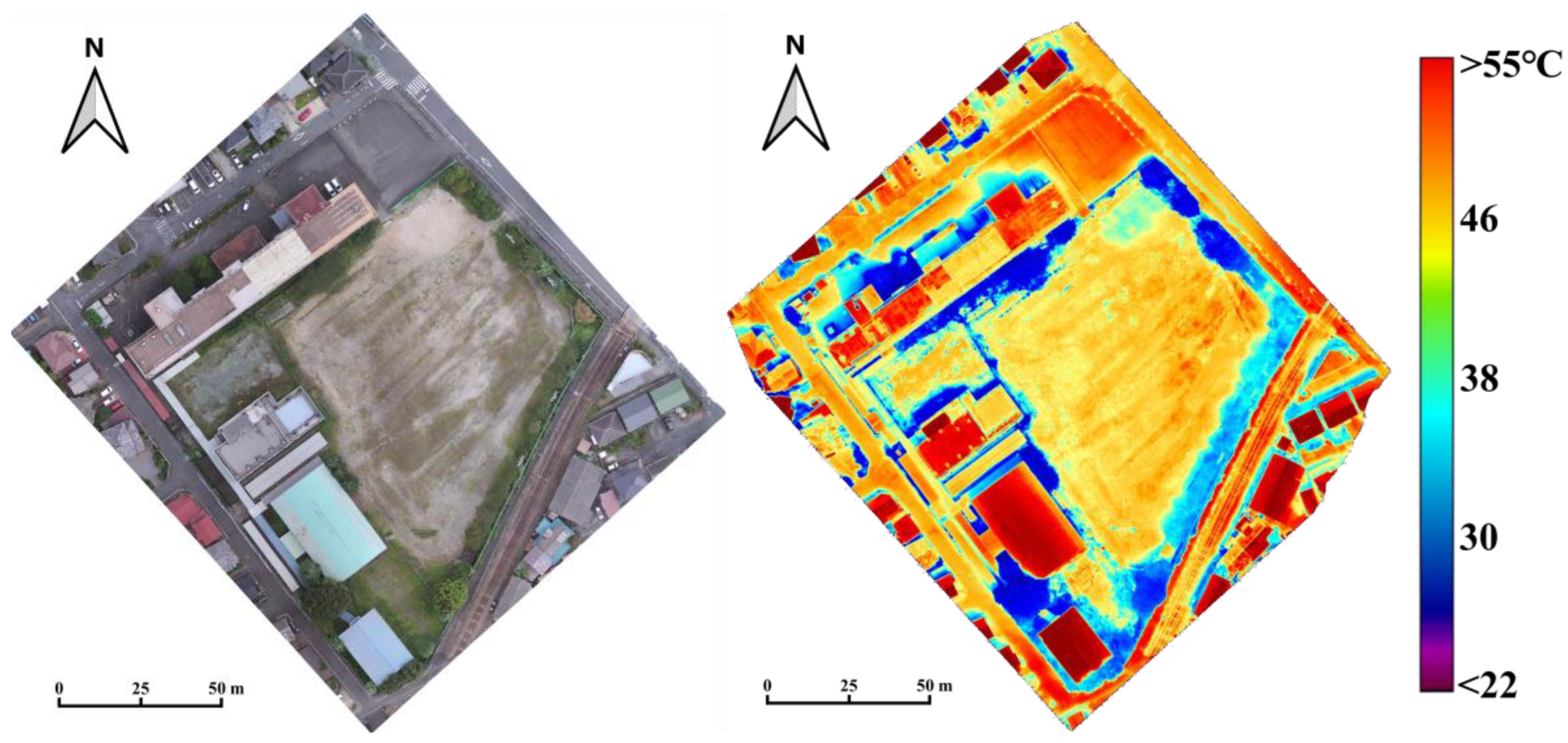
Figure 8 shows the successfully developed orthomosaic imagery of the visible and DSM for the city, orthoimage and thermal images for site 1. The ultrafine resolution of the thermal image effectively captures the trends at site 1. As expected, bare soils, asphalt, and concrete roads are much hotter than vegetated areas (e.g., trees and grassy spaces). Each building roof shows substantial heating due to direct solar radiation, with the difference in albedo clearly influencing heat absorption characteristics. Specifically, darker rooftops demonstrate higher temperatures than lighter-colored areas, such as the white rooftop on the northern building. However, despite its lighter color, the large southern building’s roof, constructed from corrugated metal (characteristic of a gymnasium hall), exhibits elevated temperatures, likely due to the material’s high heat absorption properties. Some areas on the north side behind the building show lower temperatures even though the surface material is asphalt because they lie in the shadow cast by the adjacent structures. The observation highlights the critical role of urban geometry in modulating microclimates within cities, and it is shown that detailed thermal conditions can be effectively captured through UAS remote sensing. The orthoimage of the city is also successfully generated from the aircraft data. The reconstructed 3D model (DSM) shows promising results, showing the overall elevation together with the heights of each house and building. It can be concluded that the SfM method can be applied to conventional aircraft imagery with no problems.

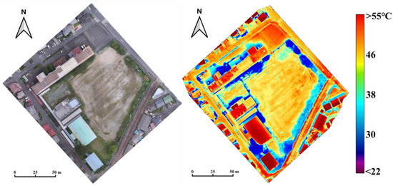
Figure 8.
Ortho mosaicked image of the city and the generated DSM (top), and orthoimage and thermal data of site 1 (bottom). The thermal data at site 1 was observed at approximately 11:00 A.M. local time.
4.2. Explanatory Variables
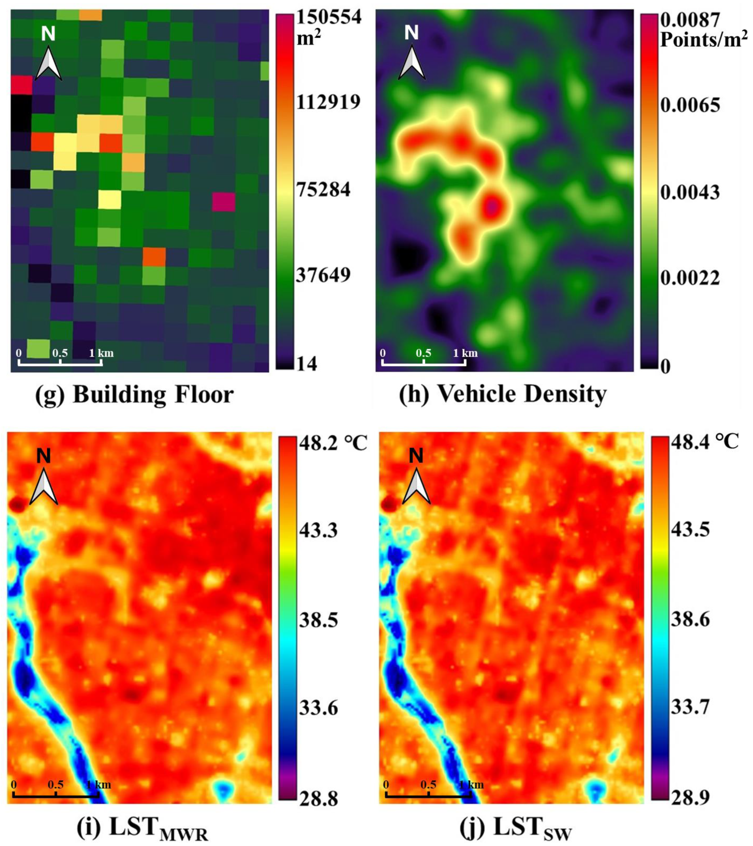
Figure 9 shows all the variables generated for the spatial modeling of the city. Solar radiation and wind exposure were computed using the 3D model (DSM) of the city. Using aircraft data made it possible to magnify the scale to what people commonly encounter during daily life while also maintaining the spatial extent. The resolution is 0.5 m, and every street and road is visible, allowing modeling of the complex conditions of the surface. It is also evident that large buildings cast shadows and block direct solar radiation. Adjusting the solar radiation time accumulation, the area can be interpreted as higher radiation or shadow areas. The NDVI and NDMI from Sentinel-2 data show a good overall trend in the study area, even when the original resolution is 10 m. Building floor data can distinguish the concentrated urbanized area within the city. Taller and larger buildings result in a greater floor area, which can be interpreted in two ways: emitting a large amount of anthropogenic heat or a source of shadows. Vehicle density was also successfully used to characterize congested areas, which can be interpreted as sources of anthropogenic heat, such as from exhaust pipes. Finally, the LST of the city is shown for comparison with the proposed LSTMWR and the LSTSW. As expected, the stray light issue from band 11 is unseen, but the values remain similar to LSTSW. Figure 10 indicates the relationship between LSTMWR and LSTSW; they match well (R2 = 0.9796 and standard error = 0.352 °C).
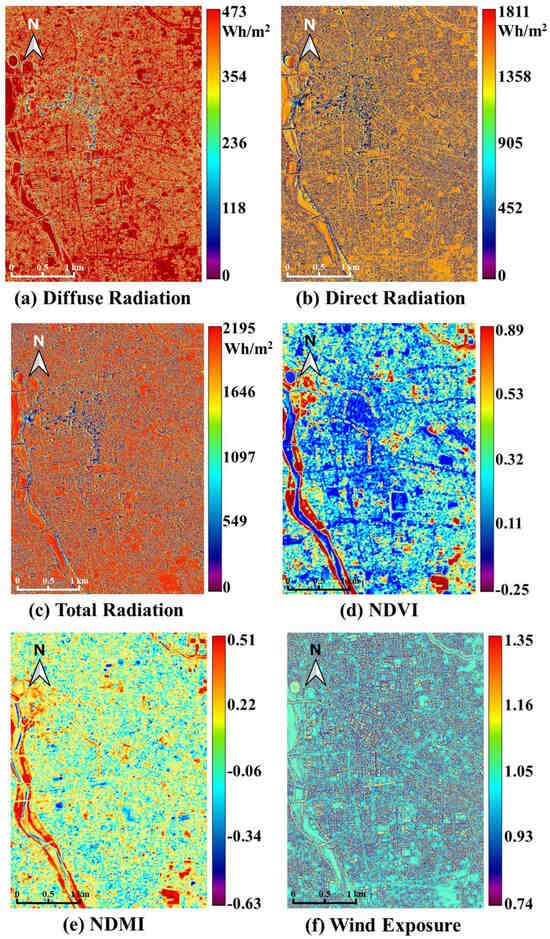

Figure 9.
Explanatory variables for the city modeling. (a) diffuse shortwave solar radiation (Wh/m2), (b) direct shortwave solar radiation (Wh/m2), (c) total shortwave solar radiation (Wh/m2), (d) normalized difference vegetation index (NDVI), (e) normalized difference moisture index (NDMI), (f) wind exposure index (g) building floor area (m2), (h) vehicle density (points/m2), (i) land surface temperature (LST) from monowindow regression (°C) and (j) LST from the split-window algorithm (°C). LSTSW is shown for comparison with the proposed LSTMWR. The stray light effects are suppressed, but the LST values are maintained as in the LSTSW.
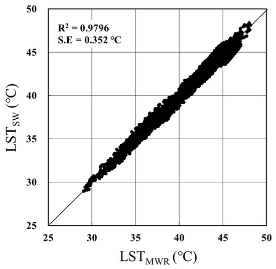
Figure 10.
Relationship between the proposed LSTMWR and LSTSW. S.E = standard error.
4.3. THI Modeling and Validation
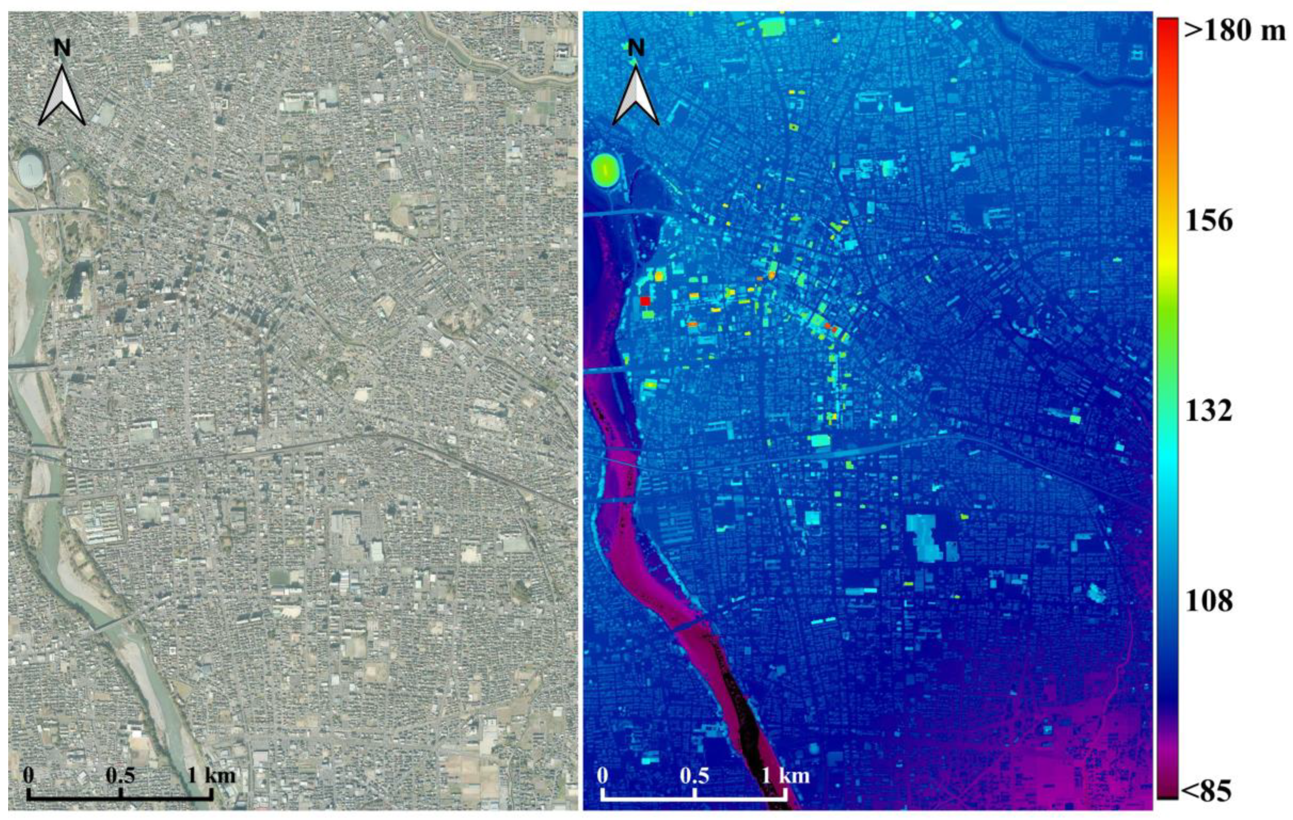
Figure 11 shows the result of mapping the THI at a microscale resolution while maintaining a large spatial extent (Modelnatural). The visual interpretation seems to represent the trends of the city effectively. For example, the tree-lined streets in the scene’s center feature lower THI values than most of the surroundings. On the other hand, the open space in front of the Maebashi station (to the north) results in a much higher THI value. This was indeed observed during the ground truthing. Small patches of parks can also be seen throughout the city, showing lower THI values. A large park with a more open grassy area was initially expected also to show similar lower THI values; however, the values of this park are higher than those of the small, patchy parks, which provides some suggestion that the lowering of the THI values is due to the existence of shadows. Therefore, the cooling effects on the SUHI are affected by LULC and the vegetation structure (i.e., trees and not grasslands). The THI distribution on the surface seems complex. For example, some areas are highly built-up areas but show lower THI values; this pattern is assumed to be caused by shadows cast by tall buildings. Such variation in the effect of the SUHI is remarkable. Nevertheless, the modeling has shown that each area has unique thermal condition characteristics, and the results can be further utilized for better urban planning. Notably, visual interpretation shows relative differences in THI values across the city; however, the values are all over 80, and the whole area features extreme conditions. This implies that we truly need to take care during the summer, even in areas that might feel relatively comfortable.
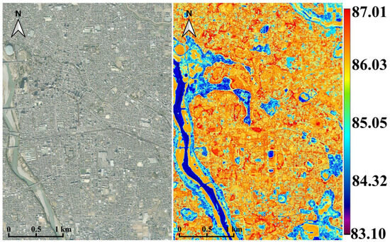
Figure 11.
THI modeling results are based on the implementation of the random forest regression. The UHI trends within the city can be clearly distinguished at a microscale level (0.5 m resolution).
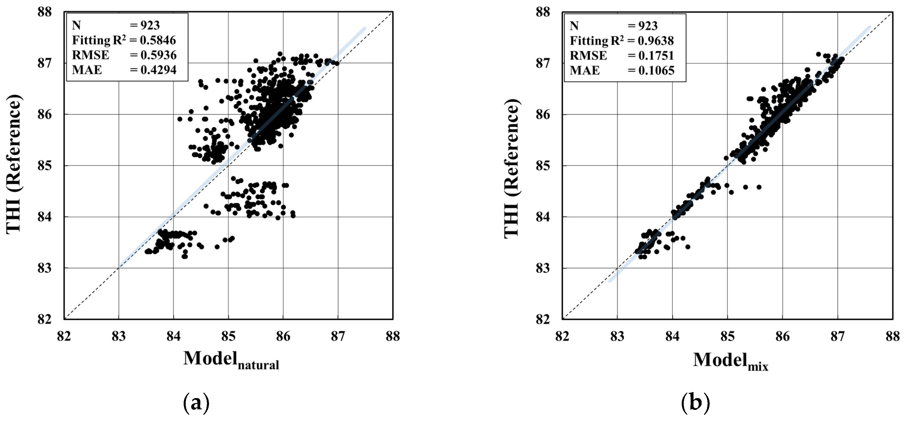
Figure 12 shows the validation results between the two developed models: Modelnatural and Modelmix. For the Modelnatural, the fitting R2 showed a moderate fit of 0.5846, the RMSE = 0.5936, and the MAE = 0.4294, slightly lower than the required R2. The larger residuals around THI < 84 are assumed to be associated with sensor lag (low response time) during ground surveying. The sensor is necessary to settle to the actual temperature and humidity; therefore, if sampling were conducted for a more limited time frame in shadow areas than entering exposed zones or vice versa, then the reference values would be slightly off from the actual values, and this was also presented by Iizuka and Akiyama [22]. The samples were collected along tree-lined streets and then in higher radiation-exposed areas. Thus, the reference would show a lower value than the modeled value. Two segments with large model errors are relevant to the following issues. First, the high residuals of THI > 85 explain why the reference set features higher THI values than the model. With natural factors only, the modeled values would be expressed as a lower THI area; however, this is not true. This is expected to be the limitation of using only natural factors that may not express the true thermal condition. It is understood that SUHIs are also affected by anthropogenic factors [23,24] along with both buildings and vehicles [10]. In fact, the works by Husni et al. [49] indicate the increase in SUHI effects with increasing traffic ques on urban streets, and Chen et al. [50] also find that vehicle heat affects significantly in areas mainly low urbanized regions with large traffic flows and highly urbanized regions with tall buildings. Therefore, the vehicles and buildings that emit heat in the city might be the remaining source for correctly modeling the THI. Second, the high residuals of the THI range of 84–85 could be from a similar issue, but in this case, the high THI model result may be suppressed by cooling effects in the city. This can be due to shadows from trees or buildings that may act as a cooling source [20]. The second model, which included anthropogenic factors, was also developed to better understand this hypothesis using vehicle density and building floor area (Modelmix). The result was remarkable, and the validation between the model and reference set showed that the residuals became much smaller. The fitting R2 = 0.9638, RMSE = 0.1751, and MAE = 0.1065. This implies that it was true that such anthropogenic factors can act as sources of both heating and cooling, depending on the area structure and the surrounding environment.
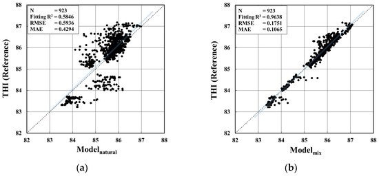
Figure 12.
Evaluation between the reference set and the modeled result. (a) Modelnatural is the developed model using only natural factors, and (b) Modelmix includes anthropogenic factors. The R2 here indicates how well the model fits the 1:1 line.
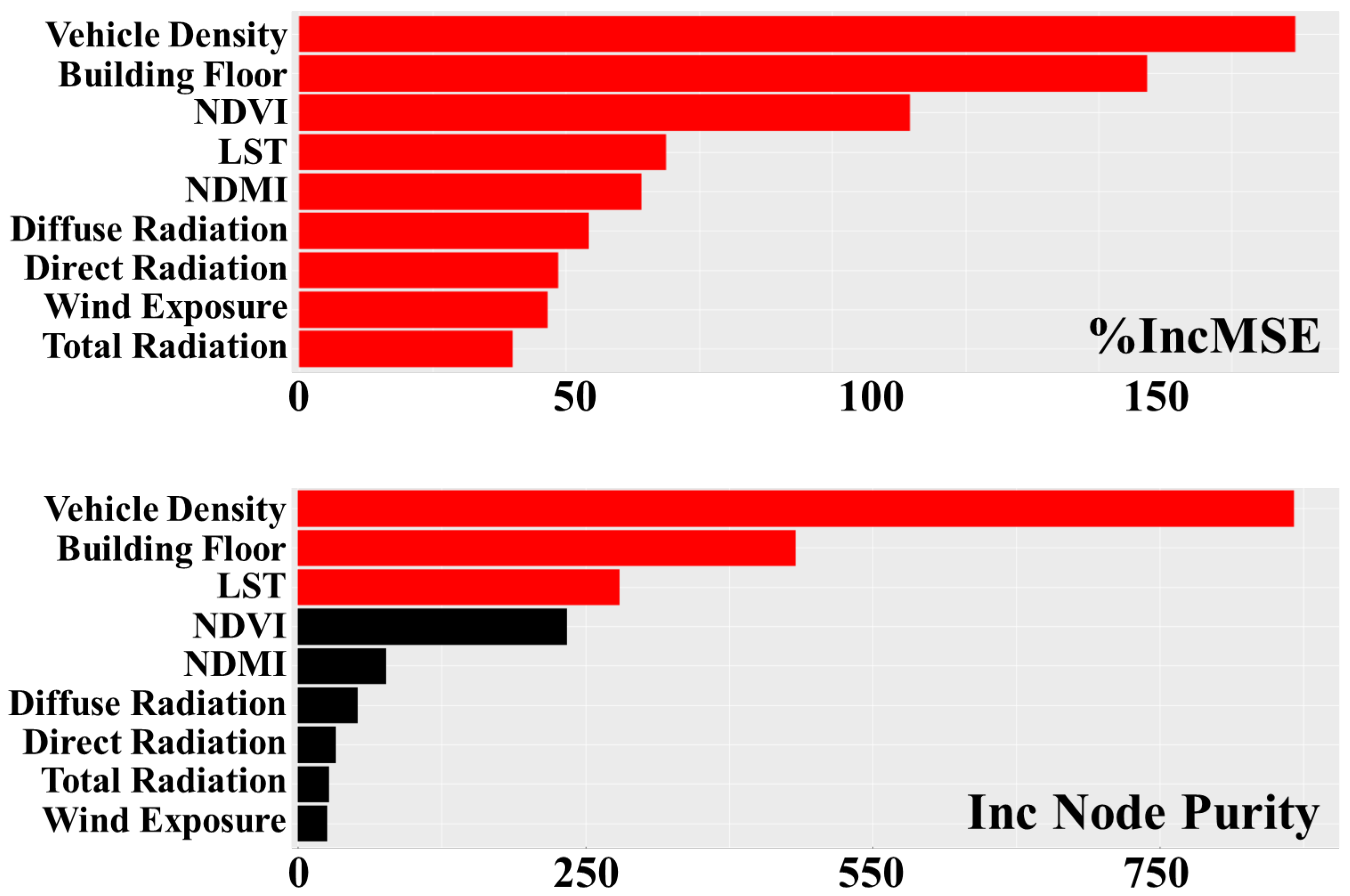
Figure 13 shows the contribution of the variables to the developed model. The two figures indicate the mean increase in node purity (Gini Index) and the percent increase in the mean squared error (%incMSE). The Gini index measures how well the variable can split a node, while the %incMSE provides an estimate of how much the accuracy will decrease when the variable is excluded. Regarding %incMSE, vehicle density has the greatest effect, followed by building floor, NDVI, LST, NDMI, diffuse radiation, direct radiation, wind exposure, and total radiation, which are all significant in terms of variable importance. For splitting the nodes, the Gini index shows higher importance for vehicle density, building floor, and LST, which are the significant variables, followed by the other variables, although these variables still provide some degree of contribution to the model. Note that the trend is checked for the SUHI and might differ for different boundary layers [20].

Figure 13.
The Importance of each variable is explained as the % increase in MSE (top) and mean increase in node purity (bottom). The red lines indicate that the variables are statistically significant (p ≤ 0.05).
5. Discussion
5.1. Improving THI Modeling through Multiplatform Data Integration
This study uses multiplatform data, including satellite, UAS, and social big data, to differentiate between natural and anthropogenic factors influencing the THI in urban environments. A key contribution of our work is the ability to map the spatial heterogeneity of THI at a fine resolution, incorporating both temperature and humidity. This reflects human discomfort more accurately than LST alone.
Our findings show that integrating social data, particularly vehicle density, significantly improves the model’s accuracy in predicting THI, addressing the over- and under-estimations observed when only natural factors were considered. This result aligns with findings from other studies, such as Husni et al. [49], who used IoT-based weather stations and vehicle detection systems to explore how high vehicular traffic contributes to localized temperature increases. Similarly, Chen et al. [50] demonstrated that vehicle heat (VH) critically impacts urban thermal environments, particularly in densely trafficked areas, contributing significantly to the SUHI effect.
The vehicle data, which is collected via GNSS positioning provides a more accurate representation of traffic patterns compared to Chen et al. [50], who used annual traffic census data and simulated vehicle flow with a cell-transmission model. While Husni et al. [49] employed the deep learning YOLO framework to count vehicles on specific streets, their approach was limited in spatial extent to areas where the equipment was installed. In contrast, our approach provided vehicle data with precise location and timing, expanding identification across a larger urban area.
5.2. Urban Geometry and Its Impact on Thermal Discomfort
Building floor area also significantly influenced our model predictions, aligning with existing research on microscale variations of the SUHI effect. Such variations are increasingly recognized as crucial for understanding urban microclimates at the level of individual streets and buildings. For example, Hu et al. [51] found that building height is inversely related to LST, with taller buildings likely suppressing LST due to shading. Hwang et al. [32] observed greater discomfort in less shaded urban streets in central Taiwan, using the sky view factor (SVF) as a response variable. Sharmin et al. [31] showed that air temperature was positively correlated with the surface-to-volume ratio of surrounding buildings in residential areas but negatively correlated when commercial and educational areas were included. This suggests that residential areas might experience higher temperatures due to greater solar exposure, while commercial areas, with more heat retention and less ventilation, could also have higher temperatures, likely due to the urban canyon effect and increased anthropogenic heat. Mughal et al. [52], although not at the microscale level, conducted a Multilayer Urban Canopy Model to simulate Singapore’s urban climate, incorporating local climate zones (LCZs) for a detailed understanding of UHI effects. They found that compact high-rise buildings intensify UHI due to trapped heat and reduced ventilation. Their study emphasized the role of anthropogenic heat, particularly from air conditioning systems, in contributing to UHI. However, their work did not incorporate vehicle data, limiting their ability to distinguish the specific impacts of different sources of anthropogenic heat.
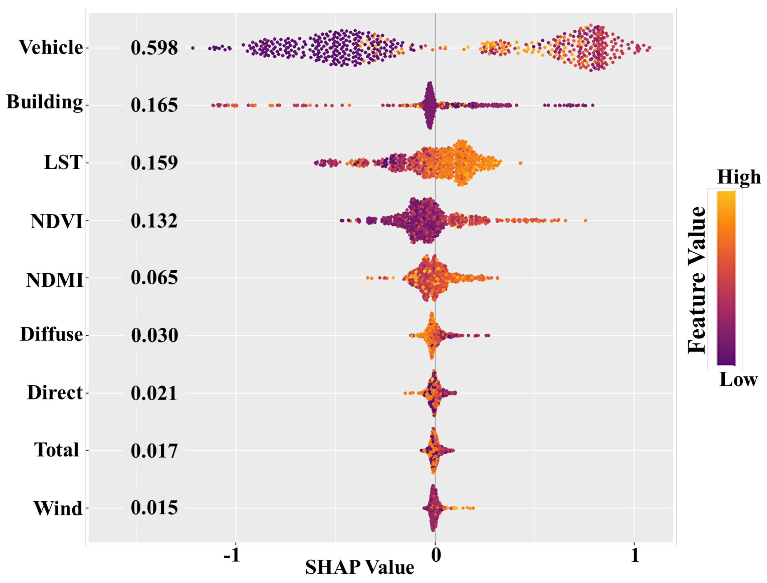
To seek in-depth of our findings, we additionally analyzed how each variable influenced the model predictions by computing SHapley Additive exPlanations (SHAP), a game-theoretic approach used to explain the output of machine learning models [53]. The variables are listed in Figure 14 in order of their influence on the model, with the color scale indicating the value of each variable and the SHAP values corresponding to the dependent variable (i.e., THI).

Figure 14.
SHapley Additive exPlanations (SHAP) summary plot. The horizontal axis represents SHAP values (influence on THI), with each dot indicating the contribution of a variable at a specific feature value from the samples. The color gradient indicates the absolute value of each variable. The vertical axis lists the variables used in the model, ordered from the most to the least influential at the top.
The analysis shows that vehicle density clearly impacts THI: higher vehicle density is associated with higher THI, and vice versa. The building floor area generally shows that a larger area reduces THI. However, there is a nuance where slightly larger building floor areas are associated with higher THI. This could align with other studies that suggest the possibility of heating influences, particularly during the daytime, from anthropogenic sources such as air conditioning [31,50]. These detailed findings are typically challenging to capture in large-scale, regional analyses of SUHIs, which often focus on broader thermal trends across wide areas. For instance, studies by Estoque and Murayama [11] and Ranagalage et al. [12] used satellite data to monitor thermal trends over large urban settings. However, as Parlow et al. [26] have noted, the thermal conditions of the urban landscape at coarser resolutions might be heavily influenced by building roofs, potentially overlooking the finer-scale variations crucial for understanding the complexities of urban microclimates.
Regarding the role of vegetation in suppressing SUHI, numerous studies have highlighted its cooling effects. However, our modeling results indicate that higher NDVI is associated with higher THI. Hofierka et al. [54] suggest that urban greenery, particularly high vegetation, significantly cools urban areas through several mechanisms, including intercepting solar radiation, providing shading, and consuming latent heat via evapotranspiration. This is a generally observed trend and is intuitively understandable. It’s important to note that THI is modeled to reflect human discomfort, incorporating both temperature and humidity. While some instances of higher NDVI are associated with lower THI due to shading effects from taller trees, we believe the relationship is more complex and may vary according to different vegetation structures. For example, while shading can reduce THI and contribute to a more comfortable environment, land use types like open grassy parks may reduce LST through evapotranspiration but increase local humidity, thus leading to higher THI. Additionally, our findings show that areas with lower diffuse radiation tend to have higher THI. This could be similar to the effects of a low SVF, where closed environments may restrict air ventilation and increase discomfort [31,32].
5.3. Microscale Urban Climate Analysis
Microscale research in SUHI studies is gaining attention, with a growing interest in detailed analysis. Cases can be seen from studies utilizing UAS and onboard thermal cameras for specific sites [18,22], as well as in the work of Lee et al. [55] and Chui et al. [56], who used handheld thermal cameras to measure street-level thermal conditions and estimate air temperature. However, our study advances this field by integrating high-resolution data from multiple platforms while maintaining a broader spatial perspective that encompasses the entire city. Recent advancements suggest that broader spatial coverage can be achieved using fixed-wing UAS [17]. However, a significant limitation of fixed-wing UAS is the extended flight time required to cover large areas, which can introduce variations in thermal conditions due to changing shortwave radiation and heat absorption during the day or longwave radiation cooling at night. Achieving a balance between high resolution and broad spatial coverage is essential for a comprehensive understanding of urban thermal environments, as it allows us to account for the variability of conditions across different urban areas. Our method addresses this challenge by employing a multi-platform approach that captures detailed information, thereby reducing the potential for time-induced discrepancies and ensuring more accurate thermal mapping.
5.4. Methodological Considerations
It is important to note that this study did not incorporate more complex indices, such as the Universal Thermal Climate Index (UTCI) [57]. While these indices provide comprehensive assessments and are better suited for capturing human bioclimatic responses, our primary objective was to map thermal indices at an extremely fine resolution using conventional satellite data and newly integrated UAS sensing data. The THI was chosen for its practicality, simplicity, and compatibility with the data sources used in our research, as it only requires temperature and relative humidity for computation. Although THI proved effective in this study, which focused on relatively low-elevation areas like Maebashi City, different outcomes may occur when applied to regions with varying elevations. Higher elevations could either overestimate or underestimate thermal discomfort in such scenarios due to different climatological conditions. The UTCI, unlike the THI, can be applied across diverse climates, seasons, and spatial scales, offering a more comprehensive assessment of thermal comfort. However, its effective application is challenging, particularly due to the difficulty and cost of accurately modeling wind velocity and mean radiant temperature, both of which are crucial for UTCI calculations. Considering the remote sensing approach, adopting absolute humidity as an alternative measure could further improve the THI model. Updating it to a more universally applicable model could significantly aid urban planners and policymakers in making informed decisions to enhance urban resilience and improve public health outcomes.
Iizuka et al. [37] discussed how finer-resolution data can significantly enhance model development at the local scale. In their forestry research, they combined UAS data with satellite imagery, which effectively boosted prediction accuracy. Our study similarly considers the benefits of integrating finer-resolution data to overcome the limitations of moderate-resolution satellite thermal data. By incorporating fine-resolution information, such as 3D city models derived from UAS or aircraft data, we can produce more precise samples to determine SUHI trends within specific urban areas, as demonstrated in our research. While the thermal data captured at larger spatial extents often limits the in-depth application of microscale SUHI analysis, our work shows that microscale trends can still be identified with moderate-resolution data. However, the results are more realistic and accurate when using finer-resolution thermal imagery. This approach offers a cost-effective alternative to more computationally intensive methods, such as supercomputing high-resolution climate simulations for urban areas [58].
UAS thermal imagery is increasingly used in environmental studies [17,18,22,59,60]; however, these platforms are often limited in spatial extent, making them challenging to apply across megacities due to local and aviation constraints. Alternatives include high-resolution thermal imaging collected by manned aircraft, as utilized by Sobrino et al. [61], but such operations can be prohibitively expensive. According to Sobrino et al. [61], a resolution greater than 50 m is necessary at the district level to accurately estimate the SUHI effect. Finer resolutions tend to exhibit higher standard deviations, likely due to anthropogenic factors, as demonstrated in our study. Acquiring thermal data at such fine resolutions citywide would be exciting and challenging, offering a valuable comparison with moderate-resolution models. Our random forest model has provided a reliable estimate of THI, demonstrating its effectiveness in this context. Additionally, random forest models are useful for downscaling LST data to finer resolutions [25]. Looking ahead, we aim to further explore past THI trends across the city and predict how they might evolve.
6. Conclusions and Future Work
This study focused on modeling the temperature-humidity index (THI) at a mi-croscale level using various remote sensing data from unmanned aerial systems (UASs), satellites, and aircraft. High-resolution aerial imagery and mosaic imagery were pro-duced from UAS and aircraft data, including both visible and thermal data. The structure from motion (SfM) method was employed to develop a 3D model of the area, from which a digital surface model (DSM) was extracted. The DSM was used to model solar radiation and wind exposure, while the normalized difference vegetation index (NDVI) and normalized difference moisture index (NDMI) were derived from Sentinel-2A satellite data. Land surface temperature (LST) was computed using Landsat 8 thermal bands. Anthropogenic factors such as vehicle density and building floor area were extracted from social big data. The random forest machine learning method utilized all these data as explanatory variables for THI modeling.
Our findings demonstrate that microscale THI trends can effectively identify potential hotspots within a city, providing critical insights for urban planning and public health interventions. The influence of anthropogenic factors on both heating and cooling effects further highlights the need to incorporate these elements into models for more accurate assessments. This approach enables the precise identification of areas at risk of high thermal discomfort, facilitating targeted interventions to mitigate SUHI effects and enhance urban resilience. The results successfully identified microscale THI trends, which are not discernible with conventional low- to moderate-resolution data, revealing potential discomfort and risk areas that could lead to health issues. This research supports environmental monitoring for smart cities and contributes to the sustainable development goals set by the United Nations. Vehicle density emerged as the most influential variable in the random forest model.
The novelty of this study lies in the integration of multiplatform remote sensing data at different resolutions and acquisition times. The mixed model showed significant accuracy with R2 = 0.9638, RMSE = 0.1751, and MAE = 0.1065 (n = 923). Future work should expand the spatial extent and consider multiple cities to reveal thermal trends contributing to SUHI. Historical trends and future possibilities will be examined, together with the consideration of state-of-the-art biometeorological indices (such as UTCI), and findings will be shared with city planners to support the development of smart cities.
Author Contributions
Conceptualization, K.I. and Y.A.; methodology, K.I.; software, K.I. and Y.A.; validation, K.I., Y.A., M.T. and T.F.; formal analysis, K.I.; investigation, K.I., Y.A., M.T., T.F. and O.Y.; resources, K.I. and O.Y.; data curation, K.I., Y.A., M.T. and T.F.; writing—original draft preparation, K.I.; writing—review and editing, K.I., Y.A., M.T., T.F. and O.Y.; visualization, K.I.; supervision, K.I.; project administration, Y.A. and O.Y.; funding acquisition, Y.A. All authors have read and agreed to the published version of the manuscript.
Funding
This research is funded by The Sumitomo Foundation Fiscal 2019 Grant (No. 184024) for Environmental Research Projects.
Data Availability Statement
The data presented in this study are available on request from the corresponding author due to data usage restrictions.
Acknowledgments
We thank the Policy Department, Creating New Value Division of Maebashi City for supporting the UAS flights in the city area.
Conflicts of Interest
Author Minaho Takase is employed by the company PASCO CORPORATION. The remaining authors declare that the research was conducted in the absence of any commercial or financial relationships that could be construed as a potential conflict of interest.
References
- Zhou, D.; Xiao, J.; Bonafoni, S.; Berger, C.; Deilami, K.; Zhou, Y.; Frolking, S.; Yao, R.; Qiao, Z.; Sobrino, J.A. Satellite remote sensing of surface urban heat Islands: Progress, challenges, and perspectives. Remote Sens. 2019, 11, 48. [Google Scholar] [CrossRef]
- Taubenböck, H.; Esch, T.; Felbier, A.; Wiesner, M.; Roth, A.; Dech, S. Monitoring urbanization in mega cities from space. Remote Sens. Environ. 2012, 117, 162–176. [Google Scholar] [CrossRef]
- Deilami, K.; Kamruzzaman, M.; Liu, Y. Urban heat island effect: A systematic review of spatio-temporal factors, data, methods, and mitigation measures. Int. J. Appl. Earth Obs. Geoinf. 2018, 67, 30–42. [Google Scholar] [CrossRef]
- Fujibe, F.; Matsumoto, J.; Suzuki, H. Regional features of the relationship between daily heat-stroke mortality and temperature in different climate zones in Japan. Sci. Online Lett. Atmos. 2018, 14, 144–147. [Google Scholar] [CrossRef]
- Ito, Y.; Akahane, M.; Imamura, T. Impact of temperature in summer on emergency transportation for heat-related diseases in Japan. Chin. Med. J. 2018, 131, 574–582. [Google Scholar] [CrossRef]
- Royé, D. The effects of hot nights on mortality in Barcelona, Spain. Int. J. Biometeorol. 2017, 61, 2127–2140. [Google Scholar] [CrossRef]
- United Nations, Department of Economic and Social Affairs, Population Division. World Urbanization Prospects: The 2018 Revision, Key Facts; Department of Economic and Social Affairs: New York, NY, USA, 2019. [Google Scholar]
- Bahi, H.; Mastouri, H.; Radoine, H. Review of methods for retrieving urban heat islands. Mater. Today Proc. 2020, 27, 3004–3009. [Google Scholar] [CrossRef]
- Voogt, J.A.; Oke, T.R. Thermal Remote Sensing of Urban Climates. Remote Sens. Environ. 2003, 86, 370–384. [Google Scholar] [CrossRef]
- Oke, T.R.; Mills, G.; Christen, A.; Voogt, J.A. Urban Heat Island. In Urban Climates; Cambridge University Press: Cambridge, UK, 2017; pp. 197–237. [Google Scholar]
- Estoque, R.C.; Murayama, Y. Monitoring surface urban heat Island formation in a tropical mountain city using Landsat data (1987–2015). ISPRS J. Photogramm. Remote Sens. 2017, 133, 18–29. [Google Scholar] [CrossRef]
- Ranagalage, M.; Estoque, R.C.; Murayama, Y. An Urban Heat Island Study of the Colombo Metropolitan Area, Sri Lanka, Based on Landsat Data (1997–2017). ISPRS Int. J. Geo-Inf. 2017, 6, 189. [Google Scholar] [CrossRef]
- Hu, Y.; Hou, M.; Jia, G.; Zhao, C.; Zhen, X.; Xu, Y. Comparison of surface and canopy urban heat Islands within megacities of eastern China. ISPRS J. Photogramm. Remote Sens. 2019, 156, 160–168. [Google Scholar] [CrossRef]
- Varentsov, M.; Konstantinov, P.; Baklanov, A.; Esau, I.; Miles, V.; Davy, R. Anthropogenic and natural drivers of a strong winter urban heat island in a typical Arctic city. Atmos. Chem. Phys. 2018, 18, 17573–17587. [Google Scholar] [CrossRef]
- Tiangco, M.; Lagmay, A.M.F.; Argete, J. ASTER-based study of the night-time urban heat island effect in Metro Manila. Int. J. Remote Sens. 2008, 29, 2799–2818. [Google Scholar] [CrossRef]
- Chang, Y.; Xiao, J.; Li, X.; Weng, Q. Monitoring Diurnal Dynamics of Surface Urban Heat Island for Urban Agglomerations Using ECOSTRESS Land Surface Temperature Observations. Sustain. Cities Soc. 2023, 98, 104833. [Google Scholar] [CrossRef]
- Dimitrov, S.; Iliev, M.; Borisova, B.; Semerdzhieva, L.; Petrov, S. UAS-Based Thermal Photogrammetry for Microscale Surface Urban Heat Island Intensity Assessment in Support of Sustainable Urban Development (A Case Study of Lyulin Housing Complex, Sofia City, Bulgaria). Sustainability 2024, 16, 1766. [Google Scholar] [CrossRef]
- Song, B.; Park, K. Verification of Accuracy of Unmanned Aerial Vehicle (UAV) Land Surface Temperature Images Using In-Situ Data. Remote Sens. 2020, 12, 288. [Google Scholar] [CrossRef]
- Aflaki, A.; Mirnezhad, M.; Ghaffarianhoseini, A.; Ghaffarianhoseini, A.; Omrany, H.; Wang, Z.H.; Akbari, H. Urban heat island mitigation strategies: A state-of-the-art review on Kuala Lumpur, Singapore and Hong Kong. Cities 2017, 62, 131–145. [Google Scholar] [CrossRef]
- Huang, X.; Wang, Y. Investigating the effects of 3D urban morphology on the surface urban heat island effect in urban functional zones by using high-resolution remote sensing data: A case study of Wuhan, Central China. ISPRS J. Photogramm. Remote Sens. 2019, 152, 119–131. [Google Scholar] [CrossRef]
- Zhao, L.; Lee, X.; Smith, R.; Oleson, K. Strong contributions of local background climate to urban heat islands. Nature 2014, 511, 216–219. [Google Scholar] [CrossRef]
- Iizuka, K.; Akiyama, Y. Assessing the micro-scale temperature-humidity index (thi) estimated from unmanned aerial systems and satellite data. ISPRS Ann. Photogramm. Remote Sens. Spat. Inf. Sci. 2020, 3, 745–750. [Google Scholar] [CrossRef]
- Ichinose, T.; Shimodozono, K.; Hanaki, K. Impact of anthropogenic heat on urban climate in Tokyo. Atmos. Environ. 1999, 33, 3897–3909. [Google Scholar] [CrossRef]
- Sailor, D.J.; Lu, L. A top–down methodology for developing diurnal and seasonal anthropogenic heating profiles for urban area. Atmos. Environ. 2004, 38, 2737–2748. [Google Scholar] [CrossRef]
- Yao, Y.; Chang, C.; Ndayisaba, F.; Wang, S. A new approach for surface urban heat Island monitoring based on machine learning algorithm and spatiotemporal fusion model. IEEE Access 2020, 8, 164268–164281. [Google Scholar] [CrossRef]
- Parlow, E.; Vogt, R.; Feigenwinter, C. The urban heat island of Basel—Seen from different perspectives. DIE ERDE J. Geogr. Soc. Berl. 2014, 145, 96–110. [Google Scholar]
- Imada, Y.; Watanabe, M.; Kawase, H.; Shiogama, H.; Arai, M. The July 2018 high temperature event in Japan could not have happened without human-induced global warming. Sci. Online Lett. Atmos. 2019, 15A, 8–12. [Google Scholar] [CrossRef]
- Nakai, S.; Itoh, T.; Morimoto, T. Deaths from heat-stroke in Japan: 1968–1994. Int. J. Biometeorol. 1999, 43, 124–127. [Google Scholar] [CrossRef]
- Kolokotroni, M.; Ren, X.; Davies, M.; Mavrogianni, A. London ‘s urban heat Island: Impact on current and future energy consumption in office buildings. Energy Build. 2012, 47, 302–311. [Google Scholar] [CrossRef]
- Imhoff, M.L.; Zhang, P.; Wolfe, R.E.; Bounoua, L. Remote sensing of the urban heat island effect across biomes in the continental USA. Remote Sens. Environ. 2010, 114, 504–513. [Google Scholar] [CrossRef]
- Sharmin, T.; Steemers, K.; Matzarakis, A. Analysis of Microclimatic Diversity and Outdoor Thermal Comfort Perceptions in the Tropical Megacity Dhaka, Bangladesh. Build. Environ. 2015, 94, 734–750. [Google Scholar] [CrossRef]
- Hwang, R.-L.; Lin, T.-P.; Matzarakis, A. Seasonal Effects of Urban Street Shading on Long-Term Outdoor Thermal Comfort. Build. Environ. 2011, 46, 863–870. [Google Scholar] [CrossRef]
- Chavez, P.S. Image-based atmospheric corrections-revisited and improved. Photogramm. Eng. Remote Sens. 1996, 62, 1025–1035. [Google Scholar]
- Iizuka, K.; Ogura, T.; Akiyama, Y.; Yamauchi, H.; Hashimoto, T.; Yamada, Y. Improving the 3D model accuracy with a post-processing kinematic (PPK) method for UAS surveys. Geocarto Int. 2021, 37, 4234–4254. [Google Scholar] [CrossRef]
- Yoo, H.; Chung, K. Heart rate variability based stress index service model using bio-sensor. Clust. Comput. 2018, 21, 1139–1149. [Google Scholar] [CrossRef]
- Morohashi, T.; Tanaka, H.; Kadowaki, T. Investigation for the ideal method of map information etc. in various foreign countries. J. Geospat. Inf. Auth. Jpn. 2010, 120, 131–147. [Google Scholar]
- Iizuka, K.; Hayakawa, Y.S.; Ogura, T.; Nakata, Y.; Kosugi, Y.; Yonehara, T. Integration of multi-sensor data to estimate plot-level stem volume using machine learning algorithms–case study of evergreen conifer planted forests in Japan. Remote Sens. 2020, 12, 1649. [Google Scholar] [CrossRef]
- Conrad, O.; Bechtel, B.; Bock, M.; Dietrich, H.; Fischer, E.; Gerlitz, L.; Wehberg, J.; Wichmann, V.; Böhner, J. System for automated geoscientific analyses (SAGA) v. 2.1. 4. Geosci. Model Dev. 2015, 8, 1991–2007. [Google Scholar] [CrossRef]
- Boehner, J.; Antonic, O. Land-surface parameters specific to topo-climatology. In Geomorphometry—Concepts, Software, Applications; Hengl, T., Reuter, H., Eds.; Developments in Soil Science; Elsevier: Amsterdam, The Netherlands, 2009; Volume 33, pp. 195–226. [Google Scholar]
- Zhang, L.; Pan, Z.; Zhang, Y.; Meng, Q. Impact of climatic factors on evaporative cooling of porous building materials. Energy Build. 2018, 173, 601–612. [Google Scholar] [CrossRef]
- Wang, L.; Lu, Y.; Yao, Y. Comparison of Three Algorithms for the Retrieval of Land Surface Temperature from Landsat 8 Images. Sensors 2019, 19, 5049. [Google Scholar] [CrossRef]
- Sobrino, J.A.; Jiménez-Muñoz, J.C.; Sòria, G.; Romaguera, M.; Guanter, L.; Moreno, J.; Plaza, A.; Martínez, P. Land surface emissivity retrieval from different VNIR and TIR sensors. IEEE Trans. Geosci. Remote Sens. 2008, 46, 316–327. [Google Scholar] [CrossRef]
- Rozenstein, O.; Qin, Z.; Derimian, Y.; Karnieli, A. Derivation of land surface temperature for Landsat-8 TIRS using a split window algorithm. Sensors 2014, 14, 5768–5780, Corrected in Sensors 2014, 14, 11277. [Google Scholar] [CrossRef]
- Qin, Z.; Karnieli, A.; Berliner, P. A mono-window algorithm for retrieving land surface temperature from Landsat TM data and its application to the Israel-Egypt border region. Int. J. Remote Sens. 2001, 22, 3719–3746. [Google Scholar] [CrossRef]
- Gerace, A.; Montanaro, M. Derivation and validation of the stray light correction algorithm for the thermal infrared sensor onboard Landsat 8. Remote Sens. Environ. 2017, 191, 246–257. [Google Scholar] [CrossRef]
- García, M.; Riaño, D.; Chuvieco, E.; Salas, J.; Danson, F.M. Multispectral and LiDAR data fusion for fuel type mapping using support vector machine and decision rules. Remote Sens. Environ. 2011, 115, 1369–1379. [Google Scholar] [CrossRef]
- Alexander, D.L.J.; Tropsha, A.; Winkler, D.A. Beware of R2: Simple, unambiguous assessment of the prediction accuracy of QSAR and QSPR models. J. Chem. Inf. Model. 2015, 55, 1316–1322. [Google Scholar] [CrossRef]
- Archer, E. rfPermute: Estimate Permutation p-Values for Random Forest Importance Metrics. R Package Version 2.1.81. Available online: https://CRAN.R-project.org/package=rfPermute (accessed on 20 May 2020).
- Husni, E.; Prayoga, G.A.; Tamba, J.D.; Retnowati, Y.; Fauzandi, F.I.; Yusuf, R.; Yahya, B.N. Microclimate Investigation of Vehicular Traffic on the Urban Heat Island through IoT-Based Device. Heliyon 2022, 8, e11739. [Google Scholar] [CrossRef]
- Chen, X.; Yang, J.; Zhu, R.; Wong, M.S.; Ren, C. Spatiotemporal Impact of Vehicle Heat on Urban Thermal Environment: A Case Study in Hong Kong. Build. Environ. 2021, 205, 108224. [Google Scholar] [CrossRef]
- Hu, Y.; Dai, Z.; Guldmann, J.-M. Modeling the Impact of 2D/3D Urban Indicators on the Urban Heat Island Over Different Seasons: A Boosted Regression Tree Approach. J. Environ. Manag. 2020, 266, 110424. [Google Scholar] [CrossRef]
- Mughal, M.O.; Li, X.-X.; Yin, T.; Martilli, A.; Brousse, O.; Dissegna, M.A.; Norford, L.K. High-Resolution, Multilayer Modeling of Singapore ‘s Urban Climate Incorporating Local Climate Zones. J. Geophys. Res. Atmos. 2019, 124, 7764–7785. [Google Scholar] [CrossRef]
- Lundberg, S.; Lee, S.-I. A Unified Approach to Interpreting Model Predictions. Adv. Neural Inf. Process. Syst. 2017, 30, 4765–4773. [Google Scholar]
- Hofierka, J.; Gallay, M.; Onačillová, K.; Hofierka, J. Physically-Based Land Surface Temperature Modeling in Urban Areas Using a 3-D City Model and Multispectral Satellite Data. Urban Clim. 2020, 31, 100566. [Google Scholar] [CrossRef]
- Lee, S.; Moon, H.; Choi, Y.; Yoon, D.K. Analyzing thermal characteristics of urban streets using a thermal imaging camera: A case study on commercial streets in Seoul, Korea. Sustainability 2018, 10, 519. [Google Scholar] [CrossRef]
- Chui, A.C.; Gittelson, A.; Sebastian, E.; Stamler, N.; Gaffin, S.R. Urban heat Islands and cooler infrastructure–measuring near-surface temperatures with handheld infrared cameras. Urban Clim. 2018, 24, 51–62. [Google Scholar] [CrossRef]
- Bröde, P.; Fiala, D.; Błażejczyk, K.; Holmér, I.; Jendritzky, G.; Kampmann, B.; Tinz, B.; Havenith, G. Deriving the Operational Procedure for the Universal Thermal Climate Index (UTCI). Int. J. Biometeorol. 2012, 56, 481–494. [Google Scholar] [CrossRef]
- Watanabe, K.; Kikuchi, K.; Boku, T.; Sato, T.; Kusaka, H. High Resolution of City-Level Climate Simulation by GPU with Multi-Physical Phenomena. In Network and Parallel Computing. NPC 2021; Cérin, C., Qian, D., Gaudiot, J.L., Tan, G., Zuckerman, S., Eds.; Lecture Notes in Computer Science; Springer: Cham, Switzerland, 2022; Volume 13152. [Google Scholar]
- Iizuka, K.; Watanabe, K.; Kato, T.; Putri, N.A.; Silsigia, S.; Kameoka, T.; Kozan, O. Visualizing the spatiotemporal trends of thermal characteristics in a Peatland plantation forest in Indonesia: Pilot test using unmanned aerial systems (UASs). Remote Sens. 2018, 10, 1345. [Google Scholar] [CrossRef]
- Melis, M.T.; Da Pelo, S.; Erbì, I.; Loche, M.; Deiana, G.; Demurtas, V.; Meloni, M.A.; Dessì, F.; Funedda, A.; Scaioni, M. Thermal remote sensing from UAVs: A review on methods in coastal cliffs prone to landslides. Remote Sens. 2020, 12, 1971. [Google Scholar] [CrossRef]
- Sobrino, J.A.; Oltra-Carrió, R.; Sòria, G.; Bianchi, R.; Paganini, M. Impact of spatial resolution and satellite overpass time on evaluation of the surface urban heat island effects. Remote Sens. Environ. 2012, 117, 50–56. [Google Scholar] [CrossRef]


Disclaimer/Publisher’s Note: The statements, opinions and data contained in all publications are solely those of the individual author(s) and contributor(s) and not of MDPI and/or the editor(s). MDPI and/or the editor(s) disclaim responsibility for any injury to people or property resulting from any ideas, methods, instructions or products referred to in the content. |
© 2024 by the authors. Licensee MDPI, Basel, Switzerland. This article is an open access article distributed under the terms and conditions of the Creative Commons Attribution (CC BY) license (https://creativecommons.org/licenses/by/4.0/).