Article

Study on Soil Moisture Status of Soybean and Corn across the Whole Growth Period Based on UAV Multimodal Remote Sensing

1
Center for Agricultural Water Research in China, China Agricultural University, Beijing 100083, China
2
National Field Scientific Observation and Research Station on Efficient Water Use of Oasis Agriculture in Wuwei of Gansu Province, Wuwei 733000, China
*
Author to whom correspondence should be addressed.
Remote Sens. 2024, 16(17), 3166; https://doi.org/10.3390/rs16173166
Submission received: 15 June 2024 / Revised: 16 August 2024 / Accepted: 23 August 2024 / Published: 27 August 2024

Abstract

:
Accurate estimation of soil moisture content (SMC) in the field is a critical aspect of precise irrigation management. The development of unmanned aerial vehicle (UAV) platforms has provided an economically efficient means for field-scale SMC measurements. However, previous studies have mostly focused on single-sensor estimates of SMC. Additionally, the lack of differentiation between various crops and their growth stages has resulted in an unclear understanding of how crop types and growth stages affect the accuracy of SMC estimation at different soil depths. Therefore, the purpose of this paper was to use UAV multimodal remote sensing and a machine learning algorithm to estimate the SMC in agricultural fields and investigate estimation’s effectiveness under different scenarios. The results indicated the following: (1) The multispectral remote sensing method provided higher accuracy in SMC estimation compared to thermal infrared remote sensing. Moreover, the integration of multimodal data improved the accuracy of SMC estimation, enhancing the coefficient of determination (R2) by approximately 14% over that achieved through the use of multispectral data alone and 39% over that of thermal infrared data alone. (2) Across the entire growth period, the optimal soil depths of SMC estimation for soybean were 10 cm and 20 cm (average R2 were 0.81 and 0.82, respectively), while for corn, they were 10 cm, 20 cm, and 40 cm (average R2 were 0.59, 0.60, and 0.55, respectively). (3) The SMC estimation model performed better for both crops during the first three growth stages, with accuracy declining in the maturity stage. These results demonstrate that this approach can provide relatively accurate root zone SMC estimates for different crops throughout their main growth periods. Thus, it can be employed for SMC monitoring and precision irrigation system design.

1. Introduction

Water resources are among the most critical assets on Earth. With the rapid development of economies and societies, water scarcity has emerged as a limiting factor hindering sustainable growth. Addressing the shortage of water resources and promoting water conservation is crucial [1]. According to China’s water resource reports over the past decade, agricultural water consumption accounts for 62.5% of annual water usage, making it the sector with the greatest potential for water conservation. The Shiyang River Basin is located in the inland region of Northwest China and experiences a continental arid temperate climate characterized by limited precipitation and high evaporation rates. Consequently, water scarcity is severe in this region [2,3]. Maintaining high and stable crop yields under such arid conditions is of paramount importance for local agricultural development. This necessitates an enhanced focus on research in water-efficient agriculture [4]. Soil moisture content (SMC) is a key variable in a climate system [5]. It represents the primary source of water uptake for plants and forms the foundational material basis for plant growth and survival [6,7]. Efficient measurement of SMC facilitates the implementation of planting and irrigation plans and holds significant implications for optimizing water resource allocation [8,9]. Current research on soil moisture has witnessed substantial advancements, spanning from observational methods to modeling techniques. Particularly noteworthy is the rapid progress in unmanned aerial vehicle (UAV) remote sensing, which offers high temporal and spatial resolution, thereby presenting possibilities for remote sensing monitoring of soil moisture at the field scale [10,11].
In the context of remote sensing for soil moisture, the divisions based on the spectral bands used can be categorized into visible-near-infrared remote sensing [12], thermal infrared remote sensing [13], and microwave remote sensing [14]. Regarding the principles of inversion, there are two main methods: the direct method and the indirect method [15].
The direct approach involves observing the soil directly and inferring its moisture content. It encompasses both the reflectance-based approach [16] and the thermal inertia method [17]. The reflectance-based approach operates on the premise that alterations in surface moisture content lead to changes in surface reflectance. Liu et al. [16] conducted sampling on ten types of soil to explore the relationship between soil reflectance in the solar domain (400~2500 nm) and SMC. Their findings indicate that under low humidity conditions, soil reflectance decreases as humidity increases, with an inverse relationship beyond a critical point, which correlates with the soil’s hydraulic properties. The thermal inertia method, based on ground temperature and thermal inertia, uses the strong linear relationship between soil moisture and thermal inertia for SMC estimation [17]. This method offers good repeatability, accuracy, and consistency. However, the thermal inertia approach is susceptible to interference from weather clouds, resulting in suboptimal soil moisture estimation outcomes in regions with dense vegetation cover or crop fields [18]. Furthermore, due to the limited penetration capability of surface radiation detected by remote sensing instruments, the soil moisture inverted using these direct methods generally represents the moisture content of the surface soil layer, typically between 5 cm and 10 cm deep, rather than the SMC in the 20–80 cm root zone [17,19,20].
The indirect method estimates soil moisture indirectly by constructing vegetation indices. It primarily relies on changes in plant physiological processes induced by drought, leading to alterations in leaf spectral properties, which significantly impact the spectral reflectance and the temperature of the vegetation canopy [21,22,23]. Yang et al. [24] extracted the temperature information for corn canopies from thermal infrared images captured by a UAV and calculated the crop water stress index (CWSI) to estimate the SMC at different depths of the cornfield. The method demonstrated effective performance, particularly at the 0–30 cm soil layer. Zhang et al. [25] extracted corn vegetation cover and canopy temperature depression (CTD) to analyze their relationship with SMC. They estimated the SMC at a depth of 0–30 cm in the corn root zone using a total of 60 data points. The results revealed high R2 values, particularly exceeding 0.71 at the 10–20 cm depth range.
Compared to the soil moisture estimation based on single remote sensing information, the joint estimation of soil moisture based on multisource remote sensing information has become a research hotspot [26,27,28]. Wigmore et al. [29] used drones equipped with visible, near-infrared, and thermal infrared sensors to obtain the temperature vegetation dryness index (TVDI). Through on-site measurements for calibration, they inferred the surface soil moisture. The R2 for the two study areas, with 13 and 15 observation points, respectively, were 0.55 and 0.76, achieving sub-meter resolution mapping of partial surface soil moisture in two former glacier valleys within Rio de Janeiro, Brazil. Cheng et al. [30] employed Landsat 8 data and the random forest regression (RFR) algorithm for multisensor combination to estimate soil moisture. The study was based on 13 remote sensing images and soil moisture data from 72 sample points corresponding to each image. The results indicate that the R2 based on the combined use of multispectral and thermal infrared indices at different soil depths ranged from 0.73 to 0.81. This was superior to the 0.69–0.73 achieved by a single multispectral sensor and the 0.67–0.74 obtained from a single thermal infrared sensor, with the differences reaching a significant level. The RFR algorithm has been successfully applied in spectral index-based soil moisture retrieval, demonstrating better accuracy and stability compared to other methods [30,31].
Most existing methods of soil moisture inversion focus on the shallow layers (0–30 cm), especially the direct methods, which can only estimate soil moisture at depths of 0–10 cm. Research on deep soil moisture is relatively limited [32]. Additionally, there is a scarcity of studies examining the differences in SMC inversion depths among different crops, and few comparisons of inversion accuracy for the same crop at different growth stages. However, the soil moisture in the crop root zone is the primary factor closely related to crop growth [33,34]. As the growth stages progress, the primary root water absorption zone of the crop may slightly shift [35,36]. Monitoring the SMC in the primary root water absorption zone at different growth stages is crucial for enhancing agricultural production efficiency and optimizing water resource management.
Therefore, the aims of this study are to (1) employ machine learning algorithms to estimate soil moisture using vegetation indices obtained from multispectral and thermal infrared remote sensing images and compare the accuracy of the SMC estimation from multimodal data, (2) use the indirect method to invert soil moisture in deeper soil layers and explore the variation pattern of SMC estimation with soil depths, and (3) analyze the impact of crop type and growth stage changes on the accuracy of soil moisture estimation.

2. Materials and Methods

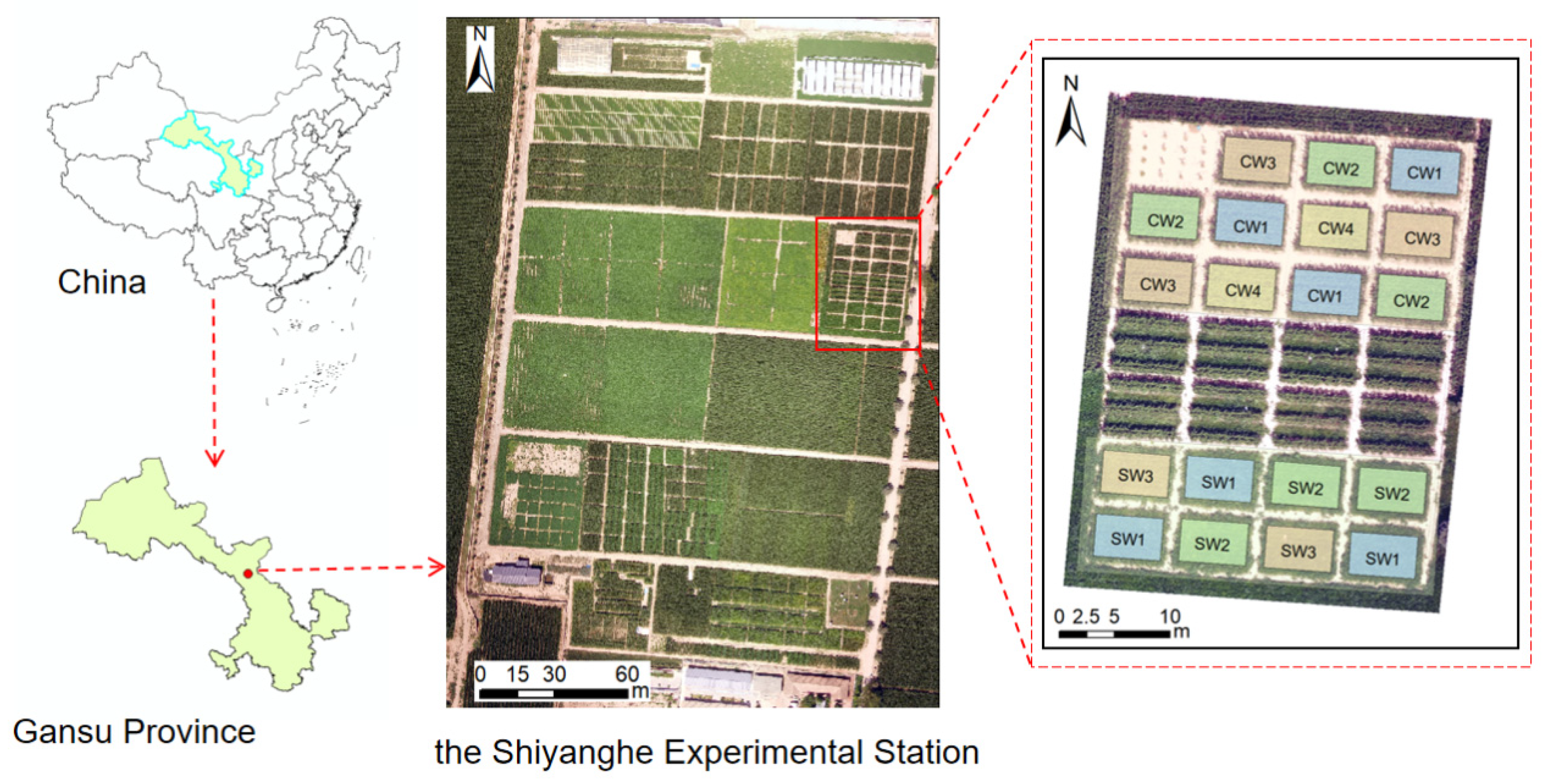
2.1. Experimental Site and Setup

The experiments were conducted at the Shiyang River Experimental Station of China Agricultural University from April to September 2022. The experimental station is located in Wangjingzhai Village, Donghe Township, Liangzhou District, Wuwei City, Gansu Province, China, at a latitude of 37°52′N and a longitude of 102°50′E. The station’s elevation is approximately 1581 m above sea level, as depicted in Figure 1. The region is characterized by an inland arid desert climate, with an average annual precipitation of 164.4 mm and potential evaporation exceeding 2000 mm. The area experiences intense solar radiation, long hours of sunshine, and a persistent lack of rainfall throughout the year, resulting in arid conditions with limited water resources. The groundwater level is approximately 40–50 m deep, further exacerbating the severe water scarcity in the area.
The field experiment covered an area of approximately 1776 square meters and was divided into 28 plots, with each plot measuring 7 m × 5 m. Isolation zones with a width of 1 m were established between the plots to prevent lateral seepage effects. The crops cultivated in the experiment were corn and soybean (Figure 1). For the corn (variety “Xianyu 335”), the rows were spaced 40 cm apart and the plants were spaced 26 cm apart. Four irrigation treatments were applied, providing 100% of the crop’s water requirement (CW1), 80% (CW2), 60% (CW3), and 40% (CW4). As for the soybean (variety “Zhonghuang 30”), the rows were spaced 50 cm apart and the plants were spaced 15 cm apart. Three irrigation treatments were implemented, corresponding to 100% of the crop’s water requirement (SW1), 75% (SW2), and 50% (SW3). Both crops were sown in early May and irrigated using the drip irrigation method with mulching. Fertilization was carried out following conventional local practices.

2.2. Data Acquisition

2.2.1. UAV Data

The remote sensing observations in this experiment were conducted using a six-axis aerial vehicle platform (DJI Matrice 600 Pro, Shenzhen, China) equipped with a thermal infrared sensor (FLIR Vue Pro R64, Wilsonville, OR, USA), a multispectral sensor (Micasense RedEdge-MX, Seattle, WA, USA), and a visible light sensor (DJI Zenmuse Z3, Shenzhen, China), as shown in Figure 2. The Matrice 600 Pro UAV has vertical and horizontal hovering accuracies of ±0.5 m and ±1.5 m, respectively. With the camera payload, the UAV has a flight time of approximately 30 min. The multispectral camera includes five spectral bands: blue (B), green (G), red (R), red edge (RE), and near-infrared (NIR). The detailed parameters of each lens are provided in Table 1.
To obtain high-resolution and full-coverage remote sensing images of the experimental field, a total of 16 UAV flight missions were conducted from 1 July to 9 September 2022. The specific dates are as follows: 1 July, 10 July, 13 July, 20 July, 22 July, 24 July, 25 July, 27 July, 31 July, 5 August, 8 August, 16 August, 19 August, 20 August, 1 September, and 6 September. The UAV flew at a height of 60 m, with a flight speed of 2 m/s, and the camera was oriented parallel to the flight path. Images were captured at regular intervals of 2 s, resulting in a longitudinal overlap rate of 92% and a lateral overlap rate of 90%. The observations were carried out on sunny and cloudless days at noon. Prior to each flight, the multispectral camera captured images of the radiometric calibration panel for radiometric correction. The emissivity of the thermal infrared camera was set to 0.98, and the background temperature was set to 22 °C.

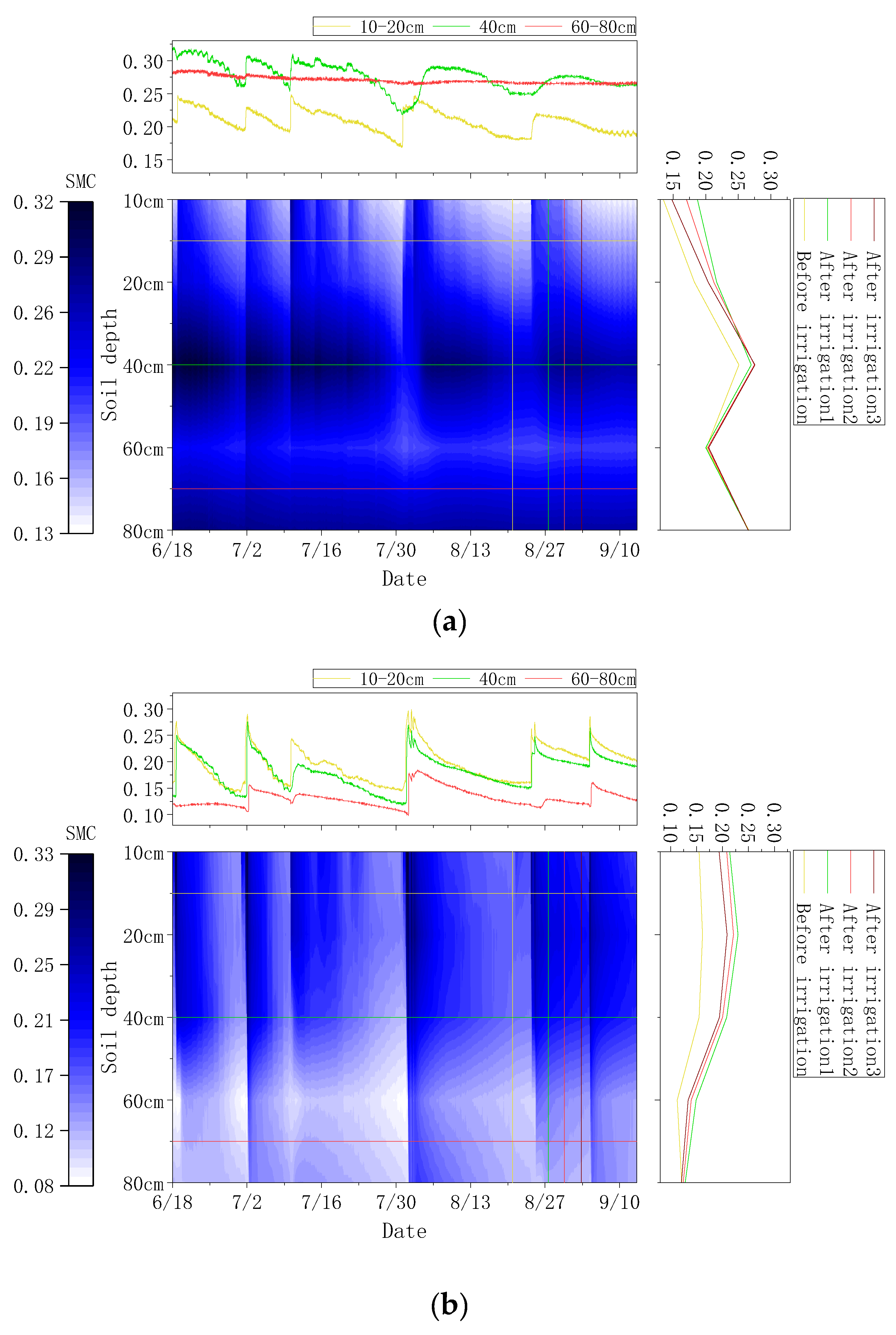
2.2.2. In Situ Soil Moisture

The soil moisture variations in different soil layers were measured using soil moisture sensors at fixed locations. In each designated plot, SMC measurements were conducted in situ. Seven 80 cm deep soil profiles were excavated in 7 small plots, and EC-5 probes (Decagon, Pullman, WA, USA) were installed at depths of 10 cm, 20 cm, 40 cm, 60 cm, and 80 cm in each profile. Data was collected at 10 min intervals by HOBO H21-USB data loggers (Onset, Cape Cod, MA, USA) and periodically downloaded for storage. Figure 3 presents the actual SMC of soybean (a) and corn (b) during the UAV flights under sufficient irrigation (SMC distribution maps for all water treatments of soybean and corn in the vertical profiles throughout the entire growth period are shown in Figures S1 and S2). In the figures, the line chart above the profile represents the variation of soil moisture at different depths over time, with the horizontal lines in the profile indicating the corresponding depths of the line chart. The line chart to the right of the profile shows the distribution of soil moisture at different depths at various times, with the vertical lines in the profile indicating the corresponding times of the line chart. For soybean, the SMC at depths of 10–40 cm exhibited significant fluctuations before and after irrigation and rainfall. After water replenishment, the SMC gradually decreased over time due to plant uptake and slow surface evaporation, while the soil moisture at depths of 60–80 cm remained relatively stable and unchanged. For corn, variations in soil moisture were observed in all soil layers, with more pronounced fluctuations at depths of 10–40 cm compared to depths of 60–80 cm.

2.3. Methods

2.3.1. Regression Model Building

The soil moisture estimation model was developed using the random forest regression (RFR) algorithm, which is based on classification trees [37]. At present, the RFR algorithm has gained widespread adoption in estimating remote sensing data and has exhibited remarkable performance [38,39,40]. The core of the RFR methodology involves employing a vast array of regression trees to explore the correlation between independent variables and the dependent variable. Each tree encapsulates a set of criteria to establish the input–output correspondence. In this study, to simulate the relationship between remote sensing indices and the SMC, a set of training input–output pairs, that is, remote sensing indices–SMC, was provided. Thus, 75% of the sample points were selected as the training set for the RFR model, and the remaining 25% were used as the testing set.
A total of 23 input variables were extracted from the multispectral and thermal infrared UAV remote sensing data (Table 2). The extracted vegetation indices were matched with the corresponding in situ SMC data for each plot. Throughout the 16-day UAV flight campaign, a total of 7 plots with 5 soil depths each were surveyed, resulting in 560 sample sets, which were used to train and validate the model developed in this study.
The normalized difference vegetation index (NDVI) images acquired from the multispectral sensor and the surface temperature (Ts) images obtained from the thermal infrared sensor were resampled and georeferenced, and then the TVDI trapezoidal feature space was constructed (Figure 4), ultimately yielding the TVDI values for each pixel. As shown in Figure 4, the dry edge and wet edge represent the highest and lowest temperatures corresponding to each NDVI, respectively, and linear fitting was performed. The R2 of the linear fitting for the dry edge and wet edge were 0.67 and 0.71, respectively, indicating a good fit.

2.3.2. Validation

The performance of the model was quantified using the coefficient of determination (R2), root mean square error (RMSE), and mean absolute error (MAE). The calculation methods for these three evaluation metrics are as follows:
R 2 = 1 i = 1 n P i O i 2 i = 1 n O i O i ¯ 2
R M S E = i = 1 n P i O i 2 n
M A E = 1 n i = 1 n P i O i
where n is the number of samples, O i is the measured moisture, P i is the estimated moisture, and O i ¯ is the mean value of O i , respectively.

3. Results

3.1. Modeling and Validation of Soil Moisture Content

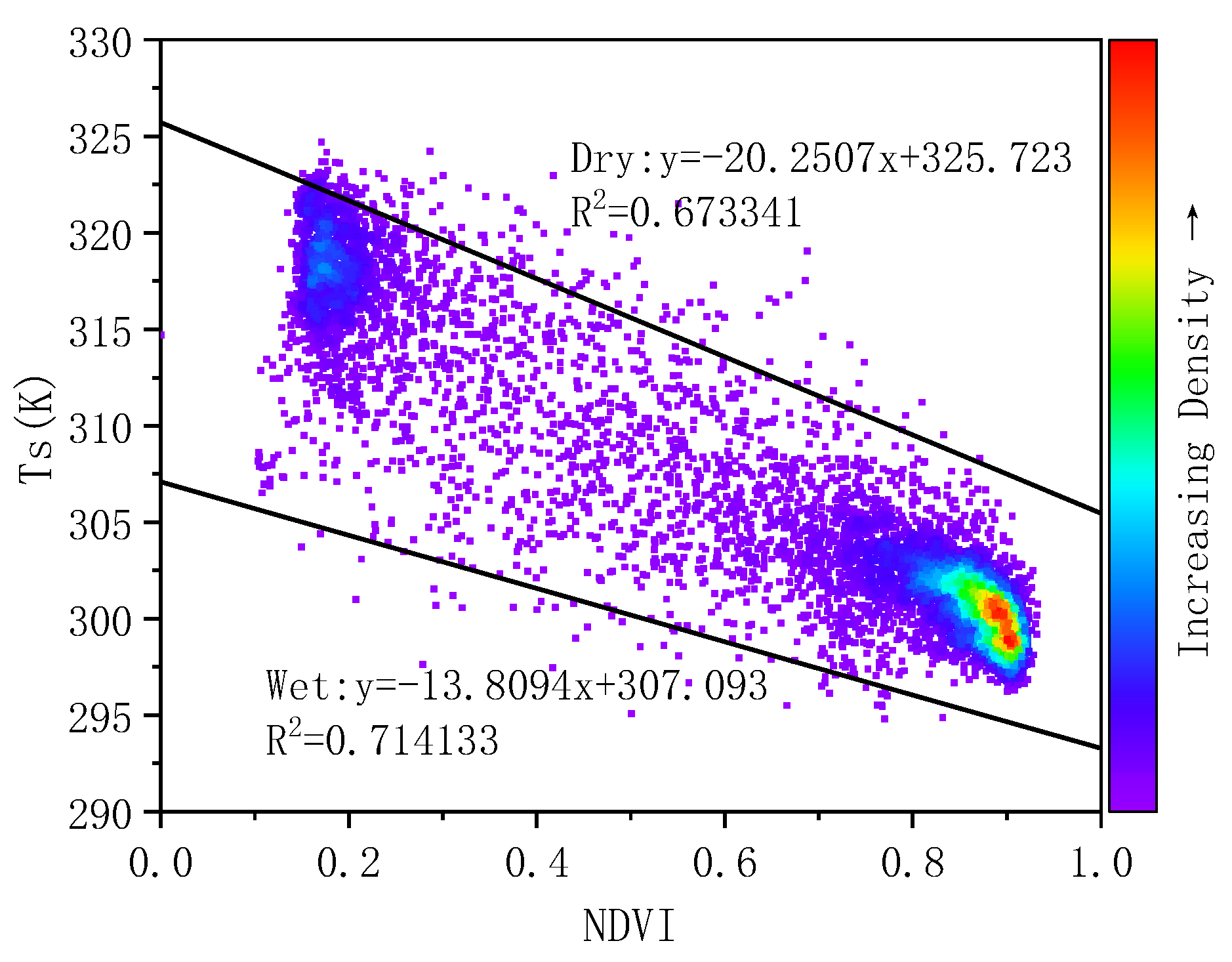
3.1.1. The Relationship between Vegetation Indices and Soil Moisture

Using the NDVI-Ts derived TVDI trapezoidal feature space, the spatial distribution map of the TVDI on July 31 and the frequency distribution histograms of each treatment plot were obtained (Figure 5). Figure 5 shows that the red areas had higher TVDI values, indicating drier soil, lower humidity, or more severe vegetation water stress. Conversely, the blue areas represented lower TVDI values, indicating wetter soil, higher soil moisture, or more abundant vegetation water supply. By comparing the frequency distribution histograms under different treatments, it can be seen that the mean TVDI values for corn followed the order CW1 = CW2 < CW3 < CW4, and for soybean, the order was SW1 < SW2 < SW3. The TVDI values showed a negative correlation with irrigation amount (Figures S1 and S2). This demonstrated the TVDI’s ability to effectively reflect crop water stress. Furthermore, it could be used to estimate soil moisture in the root zone of crops.
A correlation analysis was performed between 23 vegetation indices and in situ SMC data for both soybean and corn across their entire growth periods. As shown in Table 3, over half of the vegetation indices exhibited a highly significant correlation with in situ soil moisture, particularly at depths of 10 cm and 20 cm. This indicates the considerable potential of vegetation indices for soil moisture retrieval. Figure 6 shows the relative importance of input variables for estimating soil moisture at a depth of 20 cm using the random forest regression (RFR) model. The figure indicates that all variables have relatively high importance. Specifically, the modified chlorophyll absorption in reflectance index (MCARI), canopy temperature difference (CTD), crop water stress index (CWSI), and temperature vegetation drought index (TVDI) exhibit higher importance. However, similar to what is shown in Table 3, the differences among the various vegetation indices are not substantial.

3.1.2. Model Performance

The soil moisture at different depths across the entire growth periods of corn and soybean was used as the dependent variable. Two types of variables, namely, multispectral indices (MSs) and thermal infrared indices (TIRs), were used as the independent variables. They were separately and jointly employed for soil moisture estimation to compare the differences in the results. As shown in Table 4, there was a small difference in the R2 between the model training set and testing set, with the R2 differing by less than 0.2, indicating the stability of the model results.

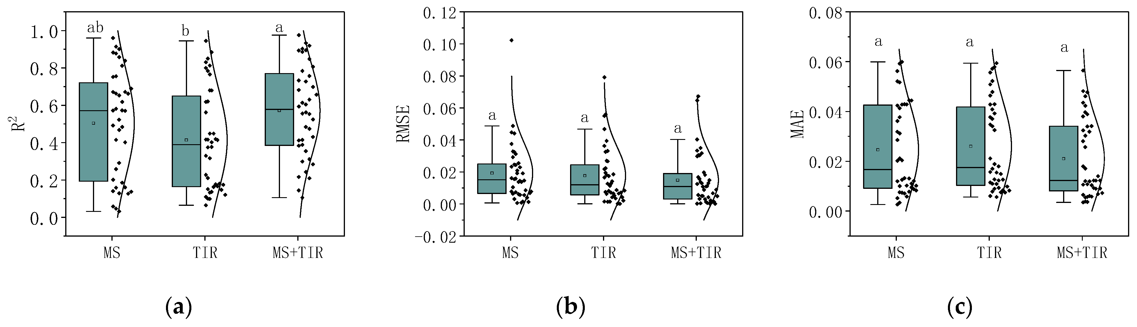
3.2. Contributions of Different Sensor Data

Crop growth stages were classified to further conduct soil moisture estimation, and the differences in accuracy were obtained for three multimodal data combinations (two individual indices and one combined index), as shown in Figure 7. Overall, for soybean and corn, at depths of 10–80 cm, the average R2 for soil moisture estimation using multispectral, thermal infrared, and multispectral + thermal infrared data were 0.50, 0.41, and 0.57, respectively. The corresponding RMSE values were 0.019, 0.018, and 0.015, and the MAE values were 0.025, 0.026, and 0.021. The results show that compared to thermal infrared, remote sensing data from the multispectral sensor provided more accurate SMC estimates with a higher R2 of approximately 0.09. The combined estimation of multispectral and thermal infrared data yielded better results than the individual estimations, with an improvement of approximately 0.07 (about 14%) compared to using multispectral alone and an improvement of approximately 0.16 (about 39%) compared to using thermal infrared alone.
Figure 8 displays the comparison of estimated and true soil moisture data at a depth of 20 cm for soybean using different sensors. It can be observed that both single-sensor and multisensor estimations tended to overestimate at low soil moisture levels and underestimate at high soil moisture levels. However, the joint use of multisensor data reduced overestimation and underestimation, providing the most accurate SMC estimates.

3.3. Comparison of Estimation Accuracy at Different Soil Depths

In addition to studying the SMC estimation using different indices, the performance of soil moisture estimation at different depths was also analyzed. Figure 9 displays the variation in SMC with soil depth for the accuracy of estimates. From the figure, it can be observed that the optimal estimation depths for soybean across the entire growth period were 10 cm and 20 cm, with average R2 of 0.81 and 0.82, RMSEs of 0.009 and 0.008, and MAEs of 0.008 and 0.006, respectively. The accuracy of estimates at depths of 10 cm and 20 cm were significantly correlated, while the accuracy for depths of 40 cm–80 cm was lower, with R2 all below 0.4 and gradually decreasing with increasing depth. As for corn, the optimal estimation depths were 10 cm, 20 cm, and 40 cm, with average R2 of 0.59, 0.60, and 0.55; RMSEs of 0.018, 0.012, and 0.009; and MAEs of 0.02, 0.015, and 0.009, respectively. The accuracy of the first three depths, especially at 20 cm and 40 cm, showed a significant correlation and the models performed well. However, the performances at depths of 60 cm and 80 cm were poorer, with R2 all below 0.3.
To further analyze the performance differences in soil moisture estimation at different depths, a correlation analysis was conducted on the in situ SMC at various soil depths, as shown in Figure 10. Overall, both soybean and corn exhibited lower correlations with the in situ SMC between distant soil layers, while adjacent soil layers showed higher correlations. For soybean, the correlation coefficient (r) between the SMC at 10 cm depth and 20 cm depth reached 0.74 (Figure 10a), reflecting a highly significant level (p < 0.01). This indicates that the SMC exhibited similar trends in response to irrigation and temporal changes at these two soil depth levels, thereby resulting in comparable accuracy in soil moisture estimation. As for corn, the r value between the SMC at depths of 20 cm and 40 cm was 0.647 (Figure 10b), reaching a highly significant level (p < 0.01), and the r value between the SMC at depths of 60 cm and 80 cm was 0.829, also reflecting a highly significant level (p < 0.01), which means that the SMC estimation accuracy was comparable in these two sets of soil layer depths, as shown in Figure 9.

3.4. Accuracy Comparison and Optimal Estimation Depths for Different Growth Stages

Figure 11 illustrates the accuracy comparison for different soil depths for both crops across different growth stages. From an accuracy perspective, both crops showed higher estimation accuracy during the first three growth stages, with a decline in accuracy during the maturity stage. The accuracy of upper soil moisture estimation for both crops (soybean 0–20 cm, corn 0–40 cm) shows significant differences between the maturity stage and other growth stages (Table 5). For corn, the decline in accuracy was particularly evident, with an average decrease in R2 of 0.35 and an increase in MAE of 0.009 compared to the first three growth stages. For soybean, the average decrease in R2 was 0.26 and the increase in MAE was 0.003.
Regarding the optimal estimation depths at different growth stages, for soybean (Figure 11a,c), the best depths for estimation during the flowering stage, podding stage, and filling stage were consistently 10 cm and 20 cm, with R2 all above 0.81. The R2 for the other three depths were all below 0.52, indicating a difference in R2 of 0.46. For corn (Figure 11b,d), the optimal estimation depths during the jointing stage, tasseling stage, and filling stage were consistently 10–40 cm, with an average R2 of 0.69. Compared to the 60–80 cm depth, the accuracy difference was 0.37. Overall, the optimal estimation depths for SMC in both crops remained relatively stable during the first three growth stages.

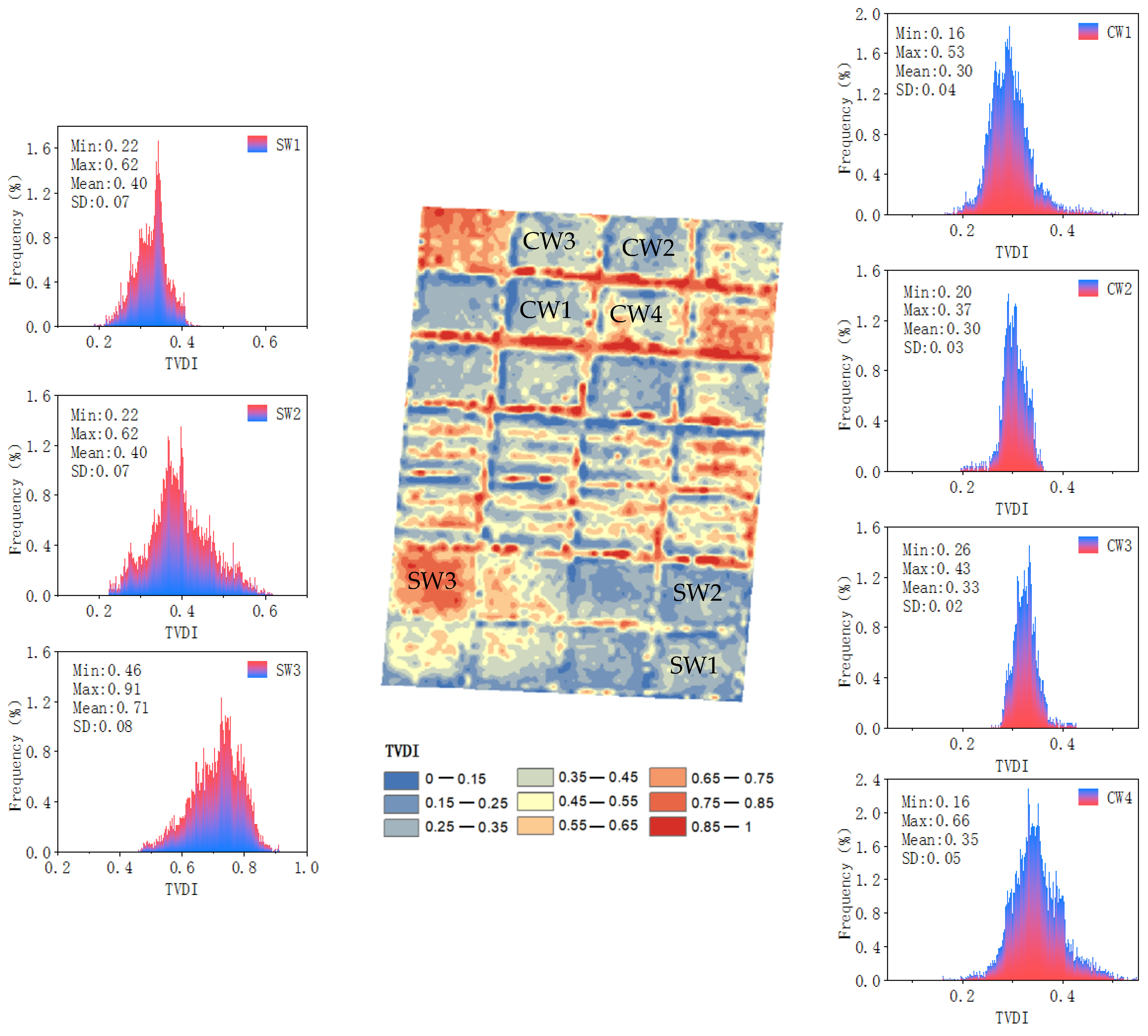
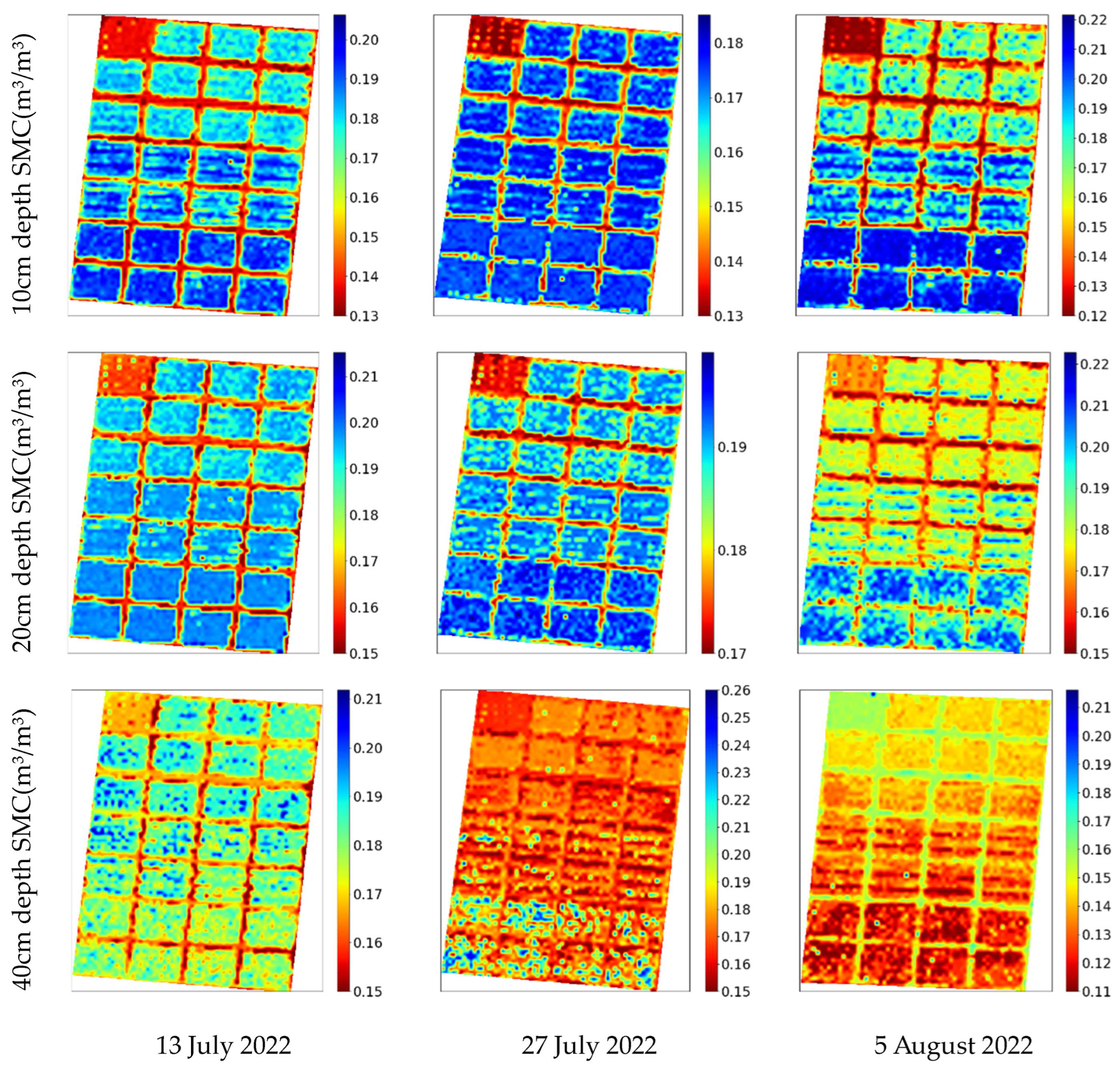
3.5. Spatial Distribution of Soil Moisture in the Field

Figure 12 shows the spatial distribution of SMC in the experimental field calculated using the RFR algorithm with a combination of multispectral and thermal infrared data as inputs. Typical days during the growth stages were selected: 13 July (soybean in the flowering stage and corn in the jointing stage), 27 July (soybean in the podding stage and corn in the tasseling stage), and 5 August (both soybean and corn in the filling stage). The spatial distribution maps of soil moisture at depths of 10 cm, 20 cm, and 40 cm on these three days were obtained. It can be observed that from 13 July to 27 July, the SMC at depths of 10 cm and 20 cm decreased for both soybean and corn, while the SMC at a depth of 40 cm decreased for corn as well. After irrigation on 1 August, the soil moisture at depths of 10 cm and 20 cm notably rebounded by 5 August. Regarding the spatial distribution, both corn and soybean, as well as different treatments of the same crop, exhibited strong spatial heterogeneity in soil moisture. Areas with higher irrigation had higher SMC, confirming the good performance of the soil moisture estimation model based on multispectral and thermal infrared remote sensing in spatial simulation.

4. Discussion

In the construction of soil moisture estimation models using remote sensing, the selection of input variables is crucial. Heavy rain reduces the differences in surface soil moisture among different treatments, and the surface soil moisture continues to experience significant temporal changes immediately after irrigation (Figure 3). Meanwhile, the vegetation growth, due to its lagging response [64], does not yet provide sufficient feedback on the soil moisture differences. Therefore, in order to reduce the impact of external disturbances, it is necessary to perform remote sensing estimation after 1–2 days of rainfall or irrigation when the soil moisture stabilizes. Moreover, images from multiple days within the same growth stage should be used together for soil moisture estimation to reduce the influence of different weather and surface conditions. Furthermore, numerous studies have shown that vegetation indices calculated using data from multispectral or thermal infrared sensors on UAVs have become the most commonly used indicators for estimating SMC [65,66]. Compared to thermal infrared sensors, multispectral sensors demonstrate superior performance in soil moisture estimation (Figure 7), while temperature data from thermal imaging can overcome the asymptotic saturation of multispectral or hyperspectral data [39] and improve the accuracy of remote sensing soil moisture estimation (Figure 6 and Figure 8). In general, joint estimation based on multispectral and thermal infrared data yields better results than individual estimations, consistent with the findings of [30].
Figure 9 displays the variation in SMC accuracy with soil depth. Overall, across the entire growth period, the optimal estimation depths for soybean were found to be 10–20 cm, while for corn, the optimal estimation depths were 10–40 cm. The model performed poorly at depths of 60–80 cm. This is because approximately 86% of soybean roots are distributed within the 0–30 cm soil depth, with the maximum root length density observed in the 10–20 cm soil layer [67]. At the same time, corn’s primary root absorption zone is deeper than that of soybean, mainly concentrated within the 0–40 cm soil depth [36]. The location of the crop’s root zone is closely related to the plant’s water uptake, which in turn is related to the plant’s growth status. Although there is a strong correlation between adjacent soil depths, such as between 20 cm and 40 cm for soybean, and between 40 cm and 60 cm for corn (Figure 10), this strong correlation is due to the water infiltration between adjacent soil layers caused by precipitation and irrigation. It does not reflect the crop’s daily water uptake from different soil layers. In reality, crops absorb less water from deeper soil layers compared to the primary root zone (10–20 cm for soybean, 10–40 cm for corn) and the moisture in deeper soil layers changes more slowly over time (Figure 3, Figures S1 and S2). For example, as shown in Supplementary Figure S1b,c, soil moisture at 40 cm, 60 cm, and 80 cm for soybean is minimally affected by external environmental conditions and thus has a lesser relationship with plant growth.
This paper also compared the accuracy of soil moisture estimation at different soil depths across different growth stages for both crops. From Figure 11 and Table 5, it can be observed that, in terms of accuracy across different growth stages, the model performed well for both crops during the first three growth stages, while it generally performed poorly during the maturity stage. This is primarily attributed to the reduction in root density during the maturity stage [68,69], as well as the yellowing and wilting of crop leaves, which weakens the relationship between vegetation indices and soil moisture across different treatment plots. Additionally, leaf shedding reduces vegetation cover, which can cause interference from the ground soil background during the extraction of canopy spectral information, thereby reducing the accuracy of the soil moisture estimation model [70]. Regarding the optimal estimation depths at different growth stages, for both soybean (Figure 11a,c) and corn (Figure 11b,d), the optimal estimation depths during the first three growth stages remain stable, with soybean at 10 cm and 20 cm, and corn at 10 cm, 20 cm, and 40 cm. This is attributed to the fact that although crop roots penetrate deeper as growth stages advance, the main rooting zones remain relatively stable over time, except during the seedling stage. Corn roots are primarily concentrated within the 0–40 cm soil depth [36,68], while soybean roots are mainly distributed around 0–20 cm soil layers [67,68], with variations depending on the crop variety and soil texture.
Section 3.1, Section 3.2, Section 3.3 and Section 3.4 demonstrate that the SMC estimation model can be applied to monitor soil moisture for different crops and their various growth stages, thereby characterizing the spatial distribution of SMC (Figure 12). We can monitor crop water consumption by observing changes in SMC. Moreover, SMC spatial distribution maps based on the model can be used to design irrigation schemes, offering greater rationality and practicality [71].

5. Conclusions

This study is based on multispectral indices and thermal infrared indices obtained through UAV remote sensing technology. These indices were applied individually and in combination using the RFR algorithm for the estimation of SMC in the 10–80 cm soil layers across different growth stages of soybean and corn. The main research findings are as follows:
(1)
For different crop growth stages and soil depths, multispectral remote sensing data outperformed thermal infrared remote sensing in terms of SMC estimation accuracy. Moreover, combining thermal infrared remote sensing data with multispectral data improved the accuracy of SMC estimation. The combined approach achieved a 14% increase in R2 compared to using multispectral data alone and a 39% increase compared to using thermal infrared data alone.
(2)
Across the entire growth period, the optimal SMC estimation depths for soybean were found to be 10 cm and 20 cm, with a significant correlation between them. The average R2 for these depths were 0.81 and 0.82, respectively. In contrast, the accuracy decreased for depths between 40 cm and 80 cm, with all R2 below 0.4. For corn, the optimal SMC estimation depths were 10 cm, 20 cm, and 40 cm, with average R2 of 0.59, 0.60, and 0.55, respectively. The performances at depths of 60 cm and 80 cm were poorer, with all R2 below 0.3.
(3)
From the perspective of different growth stages, the SMC estimation model performed well for both crops during the first three growth stages and decreased in accuracy during the maturity stage. On average, corn showed a decrease of 0.35 in R2, while soybean showed a decrease of 0.26. In terms of the optimal estimation depth across the first three growth stages, the optimal estimation depths for both soybean and corn are relatively stable, with soybean at 10 cm and 20 cm, and corn at 10 cm, 20 cm, and 40 cm.
The results indicate that using UAV remote sensing data as an input for machine learning algorithms holds promise for accurately estimating SMC in the crop root zone during growth stages other than the maturity period. The results also confirm the good performance of the model in spatial simulation, which will be valuable for guiding agricultural irrigation and improving water resource utilization efficiency.

Supplementary Materials

The following supporting information can be downloaded at: https://www.mdpi.com/article/10.3390/rs16173166/s1, Figure S1: Distribution map of soil moisture content (SMC) in vertical profiles of corn under different irrigation treatments throughout the entire growth period. (a) SW1; (b) SW2; (c) SW3; Figure S2: Distribution map of soil moisture content (SMC) in vertical profiles of corn under different irrigation treatments throughout the entire growth period. (a) CW1; (b) CW2; (c) CW3; (d) CW4.

Author Contributions

Conceptualization, Y.Z., X.Y. and F.T.; methodology, Y.Z., X.Y. and F.T.; software, Y.Z. and X.Y.; validation, X.Y. and F.T.; formal analysis, Y.Z.; investigation, Y.Z. and X.Y.; resources, F.T.; data curation, Y.Z. and X.Y.; writing—original draft preparation, Y.Z.; writing—review and editing, F.T.; visualization, Y.Z.; supervision, F.T.; project administration, F.T.; funding acquisition, F.T. All authors have read and agreed to the published version of the manuscript.

Funding

This work was supported by the National Key R&D Program of China (2022YFD190050403), the National Natural Science Foundation of China (52179049), and the Western Light-Key Laboratory Cooperative Research Cross-Team Project of Chinese Academy of Sciences (xbzg-zdsys-202103).

Data Availability Statement

The original contributions presented in the study are included in the article and Supplementary Materials, further inquiries can be directed to the corresponding author.

Conflicts of Interest

All the authors declare no conflicts of interest.

References

  1. Zhang, L.; Xia, J.; Hu, Z. Situation and problem analysis of water resource security in China. Resour. Environ. Yangtze Basin 2009, 18, 116–120. [Google Scholar]
  2. Kang, S.; Su, X.; Tong, L.; Shi, P.; Yang, X.; Abe, Y.; Du, T.; Shen, Q.; Zhang, J. The impacts of human activities on the water–land environment of the Shiyang River basin, an arid region in northwest China. Hydrol. Sci. J. 2004, 49, 413–427. [Google Scholar] [CrossRef]
  3. Kang, S.; Hao, X.; Du, T.; Tong, L.; Su, X.; Lu, H.; Li, X.; Huo, Z.; Li, S.; Ding, R. Improving agricultural water productivity to ensure food security in China under changing environment: From research to practice. Agric. Water Manag. 2017, 179, 5–17. [Google Scholar] [CrossRef]
  4. Wang, Q.; Mei, X. Strategies for Sustainable Use of Agricultural Water Resources in China. J. Agric. 2017, 7, 80–83. [Google Scholar]
  5. Seneviratne, S.I.; Corti, T.; Davin, E.L.; Hirschi, M.; Jaeger, E.B.; Lehner, I.; Orlowsky, B.; Teuling, A.J. Investigating soil moisture–climate interactions in a changing climate: A review. Earth-Sci. Rev. 2010, 99, 125–161. [Google Scholar]
  6. Luo, W.; Xu, X.; Liu, W.; Liu, M.; Li, Z.; Peng, T.; Xu, C.; Zhang, Y.; Zhang, R. UAV based soil moisture remote sensing in a karst mountainous catchment. Catena 2019, 174, 478–489. [Google Scholar]
  7. McColl, K.A.; Alemohammad, S.H.; Akbar, R.; Konings, A.G.; Yueh, S.; Entekhabi, D. The global distribution and dynamics of surface soil moisture. Nat. Geosci. 2017, 10, 100–104. [Google Scholar] [CrossRef]
  8. Lei, Z.; Hu, H.; Yang, S. A Review of Soil Water Research. Adv. Water Sci. 1999, 10, 311–318. [Google Scholar]
  9. Gago, J.; Douthe, C.; Coopman, R.E.; Gallego, P.P.; Ribas-Carbo, M.; Flexas, J.; Escalona, J.; Medrano, H. UAVs challenge to assess water stress for sustainable agriculture. Agric. Water Manag. 2015, 153, 9–19. [Google Scholar]
  10. Guo, X.; Cheng, G. Advances in the application of remote sensing to evapotranspiration research. Adv. Earth Sci. 2004, 19, 107–114. [Google Scholar]
  11. Cheng, M.; Jiao, X.; Liu, Y.; Shao, M.; Yu, X.; Bai, Y.; Wang, Z.; Wang, S.; Tuohuti, N.; Liu, S.; et al. Estimation of soil moisture content under high maize canopy coverage from UAV multimodal data and machine learning. Agric. Water Manag. 2022, 264, 107530. [Google Scholar] [CrossRef]
  12. Zhang, Z.; Wang, H.; Han, W.; Bian, J.; Chen, S.; Cui, T. Inversion of Soil Moisture Content Based on Multispectral Remote Sensing of UAVs. Trans. Chin. Soc. Agric. Mach. 2018, 49, 173–181. [Google Scholar]
  13. Guo, H.; Bu, X.; Huang, K.; Liu, Y. Inversion of soil moisture in corn field based on thermal infrared remote sensing image. J. Chin. Agric. Mech. 2020, 41, 203–210. [Google Scholar]
  14. Qiu, J.; Crow, W.T.; Wang, S.; Dong, J.; Li, Y.; Garcia, M.; Shangguan, W. Microwave-based soil moisture improves estimates of vegetation response to drought in China. Sci. Total Environ. 2022, 849, 157535. [Google Scholar] [CrossRef]
  15. Pan, N.; Wang, S.; Liu, Y.; Zhao, W.; Fu, B. Advances in soil moisture retrieval from remote sensing. Acta Ecol. Sin. 2019, 39, 4615–4626. [Google Scholar]
  16. Liu, W.; Baret, F.; Gu, X.; Tong, Q.; Zheng, L.; Zhang, B. Relating soil surface moisture to reflectance. Remote Sens. Environ. 2002, 81, 238–246. [Google Scholar]
  17. Yu, T.; Tian, G. The Application of Thermal Inertia Method the Monitoring of Soil Moisture of North China Plain Based on NOAA-AVHRR Data. J. Remote Sens. 1997, 1, 24–31. [Google Scholar]
  18. Yang, Y.; Qiu, J.; Su, H.; Tian, J.; Zhang, R. Estimation of surface soil moisture based on thermal remote sensing: Intercomparison of four methods. J. Infrared Millim. Waves 2018, 37, 459–467, 476. [Google Scholar]
  19. Wang, H.; Zhang, Z.; Fu, Q.; Chen, S.; Bian, J.; Cui, T. Inversion of Soil Moisture Content Based on Multispectral Remote Sensing Data of Low Altitude UAV. Water Sav. Irrig. 2018, 102, 90–94. [Google Scholar]
  20. Sedaghat, A.; Shahrestani, M.S.; Noroozi, A.A.; Fallah Nosratabad, A.; Bayat, H. Developing pedotransfer functions using Sentinel-2 satellite spectral indices and Machine learning for estimating the surface soil moisture. J. Hydrol. 2022, 606, 127423. [Google Scholar] [CrossRef]
  21. Zhou, Y.; Lao, C.; Yang, Y.; Zhang, Z.; Chen, H.; Chen, Y.; Chen, J.; Ning, J.; Yang, N. Diagnosis of winter-wheat water stress based on UAV-borne multispectral image texture and vegetation indices. Agric. Water Manag. 2021, 256, 107076. [Google Scholar] [CrossRef]
  22. Ren, S.; Guo, B.; Wang, Z.; Wang, J.; Fang, Q.; Wang, J. Optimized spectral index models for accurately retrieving soil moisture (SM) of winter wheat under water stress. Agric. Water Manag. 2022, 261, 107333. [Google Scholar] [CrossRef]
  23. Li, Z.; Leng, P.; Zhou, C.; Chen, K.; Zhou, F.; Shang, G. Soil moisture retrieval from remote sensing measurements: Current knowledge and directions for the future. Earth-Sci. Rev. 2021, 218, 103673. [Google Scholar] [CrossRef]
  24. Yang, S.; Chen, J.; Zhou, Y.; Cui, W.; Yang, N. A Study on the Method of UAV Thermal Infrared Remote Sensing to Retrieve Soil Moisture Content in Corn Root Zone. Water Sav. Irrig. 2021, 12–18. [Google Scholar]
  25. Zhang, Z.; Xu, C.; Tan, C.; Bian, J.; Han, W. Influence of Coverage on Soil Moisture Content of Field Corn Inversed from Thermal Infrared Remote Sensing of UAV. Trans. Chin. Soc. Agric. Mach. 2019, 50, 213–225. [Google Scholar]
  26. Zhao, Z.; Wang, H.; Qin, D.; Wang, C. Large-scale monitoring of soil moisture using Temperature Vegetation Quantitative Index (TVQI) and exponential filtering: A case study in Beijing. Agric. Water Manag. 2021, 252, 106896. [Google Scholar] [CrossRef]
  27. Ma, C.; Johansen, K.; McCabe, M.F. Combining Sentinel-2 data with an optical-trapezoid approach to infer within-field soil moisture variability and monitor agricultural production stages. Agric. Water Manag. 2022, 274, 107942. [Google Scholar] [CrossRef]
  28. Vergopolan, N.; Chaney, N.W.; Beck, H.E.; Pan, M.; Sheffield, J.; Chan, S.; Wood, E.F. Combining hyper-resolution land surface modeling with SMAP brightness temperatures to obtain 30-m soil moisture estimates. Remote Sens. Environ. 2020, 242, 111740. [Google Scholar] [CrossRef]
  29. Wigmore, O.; Mark, B.; McKenzie, J.; Baraer, M.; Lautz, L. Sub-metre mapping of surface soil moisture in proglacial valleys of the tropical Andes using a multispectral unmanned aerial vehicle. Remote Sens. Environ. 2019, 222, 104–118. [Google Scholar] [CrossRef]
  30. Cheng, M.; Li, B.; Jiao, X.; Huang, X.; Fan, H.; Lin, R.; Liu, K. Using multimodal remote sensing data to estimate regional-scale soil moisture content: A case study of Beijing, China. Agric. Water Manag. 2022, 260, 107298. [Google Scholar] [CrossRef]
  31. Ge, X.; Wang, J.; Ding, J.; Cao, X.; Zhang, Z.; Liu, J.; Li, X. Combining UAV-based hyperspectral imagery and machine learning algorithms for soil moisture content monitoring. PeerJ 2019, 7, e6926. [Google Scholar] [CrossRef] [PubMed]
  32. Babaeian, E.; Sadeghi, M.; Jones, S.B.; Montzka, C.; Vereecken, H.; Tuller, M. Ground, Proximal, and Satellite Remote Sensing of Soil Moisture. Rev. Geophys. 2019, 57, 530–616. [Google Scholar] [CrossRef]
  33. Tian, J.; Zhang, B.; He, C.; Han, Z.; Bogena, H.R.; Huisman, J.A. Dynamic response patterns of profile soil moisture wetting events under different land covers in the Mountainous area of the Heihe River Watershed, Northwest China. Agric. For. Meteorol. 2019, 271, 225–239. [Google Scholar] [CrossRef]
  34. Du, R.; Wu, J.; Tian, F.; Yang, J.; Han, X.; Chen, M.; Zhao, B.; Lin, J. Reversal of soil moisture constraint on vegetation growth in North China. Sci. Total Environ. 2023, 865, 161246. [Google Scholar] [CrossRef]
  35. Lv, Y. Maize/Soybean Intraspecific and Interspecific Competition for Resources. Ph.D. Thesis, Northwest A&F University, Xi’an, China, 2014. [Google Scholar]
  36. Bo, X.D. Simulated for Soil Water Dynamics Based on Stem Flow and Root Fractal Characteristics of Seed-Maize. Ph.D. Thesis, China Agricultural University, Beijing, China, 2016. [Google Scholar]
  37. Breiman, L. Random Forests. Mach. Learn. 2001, 45, 5–32. [Google Scholar] [CrossRef]
  38. Du, P.; Samat, A.; Waske, B.; Liu, S.; Li, Z. Random Forest and Rotation Forest for fully polarized SAR image classification using polarimetric and spatial features. ISPRS-J. Photogramm. Remote Sens. 2015, 105, 38–53. [Google Scholar] [CrossRef]
  39. Maimaitijiang, M.; Sagan, V.; Sidike, P.; Hartling, S.; Esposito, F.; Fritschi, F.B. Soybean yield prediction from UAV using multimodal data fusion and deep learning. Remote Sens. Environ. 2020, 237, 111599. [Google Scholar] [CrossRef]
  40. Rodriguez-Galiano, V.F.; Ghimire, B.; Rogan, J.; Chica-Olmo, M.; Rigol-Sanchez, J.P. An assessment of the effectiveness of a random forest classifier for land-cover classification. ISPRS-J. Photogramm. Remote Sens. 2012, 67, 93–104. [Google Scholar] [CrossRef]
  41. Rouse, J.W., Jr.; Haas, R.H.; Schell, J.A.; Deering, D.W. Monitoring vegetation systems in the great plains with erts. NASA Spec. Publ. 1973, 351, 309. [Google Scholar]
  42. Verrelst, J.; Schaepman, M.E.; Koetz, B.; Kneubühler, M. Angular sensitivity analysis of vegetation indices derived from CHRIS/PROBA data. Remote Sens. Environ. 2008, 112, 2341–2353. [Google Scholar] [CrossRef]
  43. Mishra, S.; Mishra, D.R. Normalized difference chlorophyll index: A novel model for remote estimation of chlorophyll-a concentration in turbid productive waters. Remote Sens. Environ. 2012, 117, 394–406. [Google Scholar] [CrossRef]
  44. Xue, L.; Cao, W.; Luo, W.; Dai, T.; Zhu, Y. Monitoring Leaf Nitrogen Status in Rice with Canopy Spectral Reflectance. Agron. J. 2004, 96, 135–142. [Google Scholar] [CrossRef]
  45. Broge, N.H.; Leblanc, E. Comparing prediction power and stability of broadband and hyperspectral vegetation indices for estimation of green leaf area index and canopy chlorophyll density. Remote Sens. Environ. 2001, 76, 156–172. [Google Scholar] [CrossRef]
  46. Huete, A.; Didan, K.; Miura, T.; Rodriguez, E.P.; Gao, X.; Ferreira, L.G. Overview of the radiometric and biophysical performance of the MODIS vegetation indices. Remote Sens. Environ. 2002, 83, 195–213. [Google Scholar] [CrossRef]
  47. Zarcotejada, P.; Berjon, A.; Lopezlozano, R.; Miller, J.; Martin, P.; Cachorro, V.; Gonzalez, M.; Defrutos, A. Assessing vineyard condition with hyperspectral indices: Leaf and canopy reflectance simulation in a row-structured discontinuous canopy. Remote Sens. Environ. 2005, 99, 271–287. [Google Scholar] [CrossRef]
  48. Huete, A.R. A soil-adjusted vegetation index (SAVI). Remote Sens. Environ. 1988, 25, 295–309. [Google Scholar] [CrossRef]
  49. Rondeaux, G.; Steven, M.; Baret, F. Optimization of soil-adjusted vegetation indices. Remote Sens. Environ. 1996, 55, 95–107. [Google Scholar] [CrossRef]
  50. Penuelas, J.; Frederic, B.; Filella, I. Semi-Empirical Indices to Assess Carotenoids/Chlorophyll-a Ratio from Leaf Spectral Reflectance. Photosynthetica 1995, 31, 221–230. [Google Scholar]
  51. Haboudane, D.; Miller, J.R.; Tremblay, N.; Zarco-Tejada, P.J.; Dextraze, L. Integrated narrow-band vegetation indices for prediction of crop chlorophyll content for application to precision agriculture. Remote Sens. Environ. 2002, 81, 416–426. [Google Scholar] [CrossRef]
  52. Chen, J.M. Evaluation of Vegetation Indices and a Modified Simple Ratio for Boreal Applications. Can. J. Remote Sens. 1996, 22, 229–242. [Google Scholar] [CrossRef]
  53. Wang, F.; Huang, J.; Tang, Y.; Wang, X. New Vegetation Index and Its Application in Estimating Leaf Area Index of Rice. Rice Sci. 2007, 14, 195–203. [Google Scholar] [CrossRef]
  54. Ranjan, R.; Chopra, U.K.; Sahoo, R.N.; Singh, A.K.; Pradhan, S. Assessment of plant nitrogen stress in wheat (Triticum aestivum L.) through hyperspectral indices. Int. J. Remote Sens. 2012, 33, 6342–6360. [Google Scholar] [CrossRef]
  55. Sims, D.A.; Gamon, J.A. Relationships between leaf pigment content and spectral reflectance across a wide range of species, leaf structures and developmental stages. Remote Sens. Environ. 2002, 81, 337–354. [Google Scholar] [CrossRef]
  56. Schneider, P.; Roberts, D.A.; Kyriakidis, P.C. A VARI-based relative greenness from MODIS data for computing the Fire Potential Index. Remote Sens. Environ. 2008, 112, 1151–1167. [Google Scholar] [CrossRef]
  57. Castillo-Martínez, M.Á.; Gallegos-Funes, F.J.; Carvajal-Gámez, B.E.; Urriolagoitia-Sosa, G.; Rosales-Silva, A.J. Color index based thresholding method for background and foreground segmentation of plant images. Comput. Electron. Agric. 2020, 178, 105783. [Google Scholar] [CrossRef]
  58. Sandholt, I.; Rasmussen, K.; Andersen, J. A simple interpretation of the surface temperature/vegetation index space for assessment of surface moisture status. Remote Sens. Environ. 2002, 79, 213–224. [Google Scholar] [CrossRef]
  59. Jones, H.G. Use of infrared thermography for monitoring stomatal closure in the field: Application to grapevine. J. Exp. Bot. 2002, 53, 2249–2260. [Google Scholar] [CrossRef]
  60. Jackson, R.D.; Idso, S.B.; Reginato, R.J.; Pinter, P.J., Jr. Canopy Temperature as a Crop Water Stress Indicator. Water Resour. Res. 1981, 17, 1133–1138. [Google Scholar] [CrossRef]
  61. Balota, M.; Payne, W.A.; Evett, S.R.; Peters, T.R. Morphological and Physiological Traits Associated with Canopy Temperature Depression in Three Closely Related Wheat Lines. Crop Sci. 2008, 48, 1897–1910. [Google Scholar] [CrossRef]
  62. Qiu, G.Y.; Momii, K.; Yano, T. Estimation of plant transpiration by imitation leaf temperature-Theoretical consideration and field verification(Ⅰ). Trans. Jpn. Soc. Irrig. Drain. Reclam. Eng. 1996, 183, 401–410. [Google Scholar]
  63. Qiu, G.Y.; Shi, P.; Wang, L. Theoretical analysis of a remotely measurable soil evaporation transfer coefficient. Remote Sens. Environ. 2006, 101, 390–398. [Google Scholar] [CrossRef]
  64. Yu, J.; Li, Y. Uncertainties in the usage of stable hydrogen and oxygen isotopes for the quantification of plant water sources. Acta Ecol. Sin. 2018, 38, 7942–7949. [Google Scholar]
  65. Casamitjana, M.; Torres-Madroñero, M.C.; Bernal-Riobo, J.; Varga, D. Soil Moisture Analysis by Means of Multispectral Images According to Land Use and Spatial Resolution on Andosols in the Colombian Andes. Appl. Sci. 2020, 10, 5540. [Google Scholar] [CrossRef]
  66. Lu, F.; Sun, Y.; Hou, F. Using UAV Visible Images to Estimate the Soil Moisture of Steppe. Water 2020, 12, 2334. [Google Scholar] [CrossRef]
  67. Gao, Y. Transport and Use of PAR and Water in Maize/Soybean Strip Intercropping System. Ph.D. Thesis, Chinese Academy of Agricultural Sciences, Beijing, China, 2009. [Google Scholar]
  68. Hui, F. Construction, Quantification and Evaluation of Root System Architecture and Interspecific Interaction in the Field Maize/Soybean Intercropping. Ph.D. Thesis, China Agricultural University, Beijing, China, 2020. [Google Scholar]
  69. Li, C.; Li, S.; Wang, Q.; Hou, S.; Jing, J. Effect of Different Textural Soils on Root Dynamic Growth in Corn. Sci. Agric. Sin. 2004, 37, 1334–1340. [Google Scholar]
  70. Liu, Y.; Huang, J.; Sun, Q.; Feng, H.; Yang, G.; Yang, F. Estimation of plant height and above ground biomass of potato based on UAV digital image. J. Remote Sens. 2021, 25, 2004–2014. [Google Scholar] [CrossRef]
  71. Ihuoma, S.O.; Madramootoo, C.A.; Kalacska, M. Integration of satellite imagery and in situ soil moisture data for estimating irrigation water requirements. Int. J. Appl. Earth Obs. Geoinf. 2021, 102, 102396. [Google Scholar] [CrossRef]
Figure 1. Location and layout of the experimental site.
Remotesensing 16 03166 g001
Figure 2. Schematic diagram of remote sensing observation and sensor payloads.
Remotesensing 16 03166 g002
Figure 3. Distribution map of SMC in the vertical profiles of (a) soybean and (b) corn under sufficient irrigation throughout the entire growth period.
Remotesensing 16 03166 g003
Figure 4. Depiction of the trapezoidal feature space of TVDI. The direction of the arrow indicates the gradient trend of density from low to high.
Remotesensing 16 03166 g004
Figure 5. TVDI spatial distribution map and its frequency distribution histogram.
Remotesensing 16 03166 g005
Figure 6. The relative importance of input variables in the RFR model for estimating soil moisture at a 20 cm depth.
Remotesensing 16 03166 g006
Figure 7. Accuracy of SMC estimates using different sensors: (a) R2, (b) RMSE, and (c) MAE. Significance levels are indicated by different letters: sensors with the same letter are not significantly different, while sensors with different letters are significantly different.
Remotesensing 16 03166 g007
Figure 8. Comparison of estimated and true soil moisture data for soybean at a depth of 20 cm. (a) MS, (b) TIR, and (c) MS + TIR.
Remotesensing 16 03166 g008
Figure 9. Comparison of estimation accuracy at various soil depths. (ac) Soybean and (df) Corn. Significance levels are indicated by different letters: soil depths with the same letter are not significantly different, while soil depths with different letters are significantly different.
Remotesensing 16 03166 g009
Figure 10. Correlation between the in situ SMC of different soil layer depths. (a) Soybean and (b) Corn. Note: * indicates the correlation reached significance level (p < 0.05), and ** indicates the correlation reached highly significant level (p < 0.01).
Remotesensing 16 03166 g010
Figure 11. Accuracy comparison at different soil depths across different growth stages. (a,c) Soybean and (b,d) Corn. Significance levels are indicated by different letters: soil depths with the same letter are not significantly different, while soil depths with different letters are significantly different.
Remotesensing 16 03166 g011
Figure 12. Estimation of SMC using RFR with remote sensing data from three types of sensors.
Remotesensing 16 03166 g012
Table 1. Parameters of sensors mounted on the UAV.
Sensor NameSensor TypeSpectral Region (µm)Resolution (Pixels)Field of View
(H° × V°)
RGB cameraDJI Zenmuse Z3N/A124092° (wide-angle)–35° (tele)
Multispectral cameraMicasense RedEdge-MX0.475, 0.560, 0.668,
0.717, 0.842
1280 × 96047.2° × 35.4°
Thermal cameraFlir Vue Pro R647.5–13.5640 × 51232.0° × 26°
Note: N/A—Not Applicable.
Table 2. Definitions of indicators extracted from multimodal sensor data.
SensorSpectral IndexFormulationReferences
MSNormalized difference vegetation index (NDVI)NDVI = (NIR − R)/(NIR + R)[41]
Normalized difference vegetation index 2 (NDVIgb)NDVIgb = (G − B)/(G + B)[42]
Ratio vegetation index (RVI)RVI = NIR/R[43]
Ratio vegetation index 2 (RVI2)RVI2 = NIR/G[44]
Triangular vegetation index (TVI)TVI = 60 (NIR − G) − 100(R − G)[45]
Enhanced vegetation index (EVI)EVI = 2.5 (NIR − R)/(NIR + 6 R − 7.5B + 1)[46]
Green index (GI)GI = G/R[47]
Soil-adjusted vegetation index (SAVI)SAVI = 1.5 (NIR − R) (NIR + R + 0.5)[48]
Optimized soil-adjusted vegetation index (OSAVI)OSAVI = 1.16 (NIR − R)/(NIR + R + 0.16)[49]
Structure insensitive pigment index (SIPI)SIPI = (NIR − B)/(NIR + B)[50]
Transformed chlorophyll absorption in reflectance index (TCARI)TCARI = 3[(RE − R) − 0.2(RE − G)(RE/R)][51]
Modified chlorophyll absorption in reflectance index (MCARI)MCARI = [(RE − R) − 0.2(RE − G)](RE/R)[51]
Modified simple ratio index (MSR)MSR = (NIR/R − 1)/(NIR/R + 1)1/2[52]
Green normalized difference vegetation index (GNDVI)GNDVI = (NIR − G)/(NIR + G)[53]
Simple ratio pigment index (SRPI)SRPI = B/R[50]
Normalized pigment chlorophyll index (NPCI)NPCI = (R − B)/(R + B)[54]
Plant senescence reflectance index (PSRI)PSRI = (B − R)/G[55]
Visible Atmospheric Resistant Index (VARI)VARI = (G − R)/(G + R − B)[56]
Color Index of Vegetation Extraction (CIVE)CIVE = 0.44R − 0.81G + 0.39B + 18.79[57]
TIRTemperature vegetation dryness index (TVDI)TVDI = (Ts − Tsmin)/(Tsmax − Tsmin)[58]
Crop water stress index (CWSI)CWSI = (Tc − Tw)/(Td − Tw)[59]
Canopy temperature depression (CTD)CTD = Tc − Ta[60,61]
Vegetation transpiration coefficient (hac)hac = (Tc − Ta)/(Tcp − Ta)[62,63]
Note: B—Blue band; G—Green band; R—Red band; RE—Red edge band; and NIR—Near-infrared band; Ts—Surface temperature; Tc—Canopy temperature; Tw—Wet reference surface temperature; Td—Dry reference surface temperature; Ta—Air temperature; Tcp—Reference canopy temperature.
Table 3. Pearson coefficient between vegetation index and soil moisture.
SensorSpectral Indexd10 cmd20 cmd40 cmd60 cmd80 cm
MSCIVE−0.245 **−0.240 **−0.089 **−0.155 **−0.460 **
EVI0.257 **0.225 **0.129 **0.074 *0.281 **
GI0.310 **0.136 **0.059 *0.154 **0.499 **
GNDVI0.084 **−0.091 **0.032−0.060 *−0.014
MCARI0.339 **0.215 **0.067 *0.185 **0.642 **
MSR0.253 **0.142 **0.075 **0.0430.225 **
NDVI0.106 **−0.0470.03700.116 **
NDVIgb0.373 **0.199 **−0.0050.192 **0.631 **
NPCI−0.070 *0.024−0.081 **−0.009−0.081 **
OSAVI0.219 **0.154 **0.100 **0.0520.224 **
PSRI0.084 **−0.0180.060 *0.0240.128 **
RVI0.312 **0.112 **0.078 **0.090 **0.367 **
RVI20.137 **−0.0520.047−0.0490.02
SAVI0.314 **0.297 **0.157 **0.101 **0.396 **
SIPI0.212 **−0.0160.0190.0230.248 **
SRPI−0.356 **−0.238 **−0.01−0.117 **−0.471 **
TCARI−0.112 **−0.105 **−0.010.0530.01
TVI0.289 **0.266 **0.141 **0.093 **0.352 **
VARI0.242 **0.073 *0.0520.104 **0.390 **
TIRTVDI0.0440.217 **0.106 **0.063 *−0.01
CTD−0.211 **−0.139 **−0.0540.029−0.001
CWSI−0.170 **0.167 **0.097 **−0.053−0.454 **
ha−0.132 **−0.145 **0.016−0.05−0.301 **
Note: * indicates correlation at a significance level of 0.05 and ** indicates correlation at a significance level of 0.01.
Table 4. Comparison of soil moisture estimation accuracy of different crops at different depths.
Training SetTesting Set
10 cm20 cm40 cm60 cm80 cm10 cm20 cm40 cm60 cm80 cm
soybeanMSR20.820.880.470.360.420.740.780.380.280.34
RMSE (%)0.0110.1330.0940.4080.222.6690.2251.0490.0151.1
TIRR20.820.820.280.290.240.740.720.030.010.08
RMSE (%)0.0170.0210.3320.0680.0240.2480.3098.132.0260.672
MS + TIRR20.820.890.530.360.420.780.850.460.260.32
RMSE (%)1.160.9890.5981.6980.150.5290.2080.9281.8781.266
cornMSR20.530.810.820.320.320.330.670.680.150.14
RMSE (%)0.4810.2230.0570.5040.822.582.8971.6371.0373.687
TIRR20.430.790.750.330.310.260.610.60.190.14
RMSE (%)0.1520.3510.1640.2730.1732.4763.3871.0453.7931.823
MS + TIRR20.550.850.890.40.420.40.70.730.240.28
RMSE (%)0.4330.0320.0090.7380.8211.2870.5711.3172.3777.589
Table 5. Comparison of soil moisture estimation accuracy of different crops at different growth periods.
Growth PeriodR2MAE
Soybean
(10–20 cm)
Flowering stage0.92 ± 0.05 a0.006 ± 0.002 ab
Podding stage0.84 ± 0.12 a0.005 ± 0.002 b
Filling stage0.86 ± 0.04 a0.008 ± 0.002 ab
Maturity stage0.63 ± 0.11 b0.01 ± 0.004 a
Corn
(10–40 cm)
Jointing stage0.79 ± 0.07 a0.011 ± 0.005 c
Tasseling stage0.56 ± 0.13 b0.012 ± 0.003 c
Filling stage0.72 ± 0.09 a0.014 ± 0.004 ab
Maturity stage0.24 ± 0.09 c0.022 ± 0.014 a
Note: Significance levels are indicated by different letters: growth periods with the same letter are not significantly different, while growth periods with different letters are significantly different.
Disclaimer/Publisher’s Note: The statements, opinions and data contained in all publications are solely those of the individual author(s) and contributor(s) and not of MDPI and/or the editor(s). MDPI and/or the editor(s) disclaim responsibility for any injury to people or property resulting from any ideas, methods, instructions or products referred to in the content.

