Generalization of the Synthetic Aperture Radar Azimuth Multi-Aperture Processing Scheme—MAPS

Abstract

This paper analyzes the advantages and the drawbacks of using the Synthetic Aperture Radar (SAR) azimuth multichannel technique known as Multi-Aperture Processing Scheme (MAPS), in a set of relevant application cases that are far from the canonical ones. In the scientific literature on this topic, equally distributed azimuth channels with the quasi-monostatic deployment are assumed. With this research, we aim at extending the models from the current literature to (i) a generic bistatic acquisition geometry, (ii) a set of cases where the number of receiving tiles is not the same for each channel, or (iii) the tiles are shared between adjacent channels thus creating an overlapping configuration. The paper introduces the mathematical models for the listed non-conventional MAPS cases. Dealing with the bistatic MAPS, we first solve the problem by interpreting multichannel acquisition as a bank of Linear Time Invariant (LTI) filters. Then, a more physical approach, based on discrimination of the direction of arrivals (DoAs) is pursued. The effectiveness of the two methods and the advantages of the second approach on the first are proved by using a simplified 1D end-to-end simulation. Even limiting to the monostatic configuration, the azimuth antenna tiles have always been supposed equally partitioned among the RX channels. Overcoming this limit has two advantages: (i) more MAPS possible solutions in case few azimuth tiles are available, as in the ROSE-L mission; (ii) the number of channels can be designed independently of the number of tiles, also allowing asymmetric solutions, useful for a phase array antenna with an odd number of tiles such as in the SAOCOM-1 mission. Conversely, sharing one or more receiving tiles in different receiving channels makes the input noise partially correlated. The drawback is an increase in the noise level. A trade-off is determined for the different solutions obtained using simulations with real mission parameters. The theoretical performance and the end-to-end simulations are compared.

1. Introduction

The azimuth Multiple-Aperture Processing Scheme (MAPS) is a digital beamforming processing technique that allows the reduction in the acquisition Pulse Repetition Frequency (PRF) of the Synthetic Aperture Radar (SAR), keeping the same azimuth resolution and ambiguity rejection. The advantage is the so-called High-Resolution Wide-Swath condition [1]. Next-generation SAR missions such as Sentinel-1 NG [2] and ROSE-L [3] will implement the MAPS.

When the MAPS is adopted, the SAR PRF can be decreased since the acquisition is performed through multiple channels. In this configuration, sub-parts of the antenna acquire on N different phase centers, each referring to a specific ADC, to create N SAR data. This acquisition scheme allows a higher $PR{I}_i=1/PR{F}_i$ during the data collection and then a longer Sampling Window Length (SWL) extension to gather a wider ground swath. At the same time, thanks to the general sampling theorem, the reconstruction of the full bandwidth at the higher sampling frequency is ensured by a proper on-ground recombination of the different digital acquisitions:

$$PR{F}_N={\displaystyle \frac{N}{PR{I}_i}}=N·PR{F}_i$$

(1)

This way, the azimuth ambiguities can be kept low thanks to the spectrum’s unambiguous reconstruction [4,5].

No MAPS SAR sensor has yet been mounted on operational spaceborne missions. This means that actual MAPS performance is yet to be proven, especially in the presence of realistic or possible impairments. The MAPS reconstruction requires accurate knowledge of the phase centers’ position at the wavelength order [6]. While this is not a concern for a monostatic system, it may become quickly critical for bistatic and multistatic missions put in close formation [5,6,7].

In this paper, we present a general approach for the MAPS reconstruction that goes beyond the formulation valid for a single-platform and zero Doppler (SP-ZD) instrument [1,4,5,8,9,10]. Namely, we consider the extension of the MAPS to (i) bistatic acquisition geometry, and to (ii) those cases where the number of receiving tiles is not the same for each channel, or (iii) the tiles are shared between adjacent channels, thus creating an overlapping configuration of the digital channels. To be consistent with other studies on MAPS, the Azimuth-Ambiguity-to-Signal Ratio (AASR) mitigation of the multichannel system with respect to the single-channel data is monitored. The AASR reduction is inherent to the MAPS algorithm because of the increase in the PRF in the final data. Moreover, the thermal noise level after reconstruction is also evaluated according to [5].

This paper is organized as follows. Section 2 recalls the canonical MAPS theory as presented in the literature. Successively, the paper is structured into two parts: the first presents the extension of the MAPS for bistatic missions; the second instead deals with the MAPS for monostatic, non-conventional cases. In the first part: Section 3 is devoted to the mathematical modeling of the MAPS for bistatic missions, and Section 4 presents the main results for this case using simulations. In the second part, Section 5 is for the mathematical modeling of monostatic cases with a non-equal number of tiles per MAPS channel or overlapping channels. Two real satellite systems cases are considered to feed an end-to-end simulation; the achieved results are presented in Section 6. Finally, Section 7 gives the outlook of the paper recalling the main results of the two analyzed topics.

2. Canonical MAPS Theory

In Multiple-Aperture Processing Scheme (MAPS) SAR, the antenna is used as a whole for transmission (thus maximizing the peak transmitted power) but is partitioned along azimuth by grouping tiles to create multiple receiver channels. The feasibility of such multichannel but still monostatic SAR has been widely addressed in the literature [1,5,8,9,10].

In the more recent literature, the multichannel approach has been extended to close formations of small satellites deployed in along-track convoys [5,6,7] where the distance between the Tx and the Rxs is in the order of a few hundred meters.

In the following sub-sections, we want to summarize the assessed theory of MAPS for single-platform systems (Section 2.1) and then point out its limitations (Section 2.2).

2.1. Recall of Canonical MAPS Problem

The literature on single-platform MAPSs is based on the monostatic assumption for which the results are reliable if the distance between the phase centers of transmitter and receivers is orders of magnitude smaller than the target–sensor distance. According to this hypothesis, the relation between the monostatic signal $s_{MAPS}\left(t\right)$ and the signal received by each of the N receiving channels $s_j\left(t\right)$ can be approximated (using the Taylor series expansion of the SAR hodograph around its vertex) by (i) a constant phase shift and (ii) a time delay. Both these terms depend on the physical distance $\Delta x_j$ between the phase center of the receive channels, by the following relations [1,8]:

$$\begin{array}{cc}\hfill \Delta t_j& ={\displaystyle \frac{\Delta x_j}{2v_s}}\hfill \\ \hfill \Delta {\phi }_j& =-{\displaystyle \frac{\pi \Delta x_j^2}{2\lambda R_0}}\hfill \end{array}$$

(2)

The general Impulse Response Function (IRF) of the $j^{th}$ channel ($h_{s,j}\left(t\right)$) can be written as a function of the monostatic IRF ($h_s\left(t\right)$) convolved by the time response of the LTI filter ($g_j\left(t\right)$), whose phase and delay are defined in Equation (2):

$$\begin{array}{cc}\hfill h_{s,j}\left(t\right)=& h_s\left(t\right)\ast g_j\left(t\right)\hfill \\ \hfill & h_s\left(t\right)\ast \{e^{j\Delta {\phi }_j}·\delta \left(t-\Delta t_j\right)\}\hfill \end{array}$$

(3)

Then, the signal from the $j^{th}$ channel is:

$$\begin{array}{cc}\hfill s_j\left(t\right)=& h_{s,j}\left(t\right)\ast s_{MAPS}\left(t\right)\hfill \\ \hfill & \left[h_s\left(t\right)\ast g_j\left(t\right)\right]\ast s_{MAPS}\left(t\right)\hfill \end{array}$$

(4)

Equivalently, Equation (3) can be written in the frequency domain as the product of the Fourier Transform (FT) of each term (capital letters are used to address the FT of the time-domain function, e.g., $G\left(f\right)=FT\left\{g\left(t\right)\right\}$):

$$H_{s,j}\left(f\right)=H_s\left(f\right)·G_j\left(f\right)$$

(5)

From Equation (5), it is straightforward to derive the definition of the transfer function relating the monostatic and the multichannel systems:

$$G_j\left(f\right)={\displaystyle \frac{H_{s,j}\left(f\right)}{H_s\left(f\right)}}$$

(6)

By taking the Fourier Transform of Equation (3), Equation (6) can be written as:

$$\begin{array}{cc}\hfill G_j\left(f\right)& ={\displaystyle \frac{H_{s,j}\left(f\right)}{H_s\left(f\right)}}\hfill \\ \hfill & =exp\left(-j2\pi {\displaystyle \frac{f}{v_s}}{\displaystyle \frac{\Delta x_j}{2}}\right)·exp\left(-j\pi {\displaystyle \frac{\Delta x_j^2}{2\lambda R_0}}\right)\hfill \end{array}$$

(7)

In the previous equation, the first exponential term represents the propagation delay due to the physical distance $\Delta x_j$ while the second exponential term is a constant, pure-phase term that depends again on $\Delta x_j$.

The SAR data from the different channels are combined on the ground to get the full spectrum reconstruction. In the following, we refer to the derivation of the mathematical model presented in [5] that formalizes the result in Equation (7) by using a matrix notation. This is possible because, along the azimuth, SAR is a time-discrete system, and SAR data are a sequence of samples. The observation vector $\underline{S}$ is the collection of the signals acquired by all the N receivers for the K$PRI$ of the acquisition. Then, its size is $N·K\times 1$. Considering Equation (7) and the spectrum of the target $\underline{D}$, we can write:

$$\underline{S}=\underline{\underline{G}}·\underline{D}$$

(8)

The matrix $\underline{\underline{G}}$ is the design matrix where each element is derived from Equation (7). In particular, it has as many rows as the number of receivers N times the Doppler wavenumber bins K, and as many columns as the number of PRF intervals we want to unfold. Here, we unfold the maximum number of PRF so the matrix $\underline{\underline{G}}$ has N columns.

The goal is to estimate $\underline{D}$ having as observable the vector $\underline{S}$. To do this, Equation (8) is inverted for each Doppler frequency [5]. The inversion can be pursued by using the Least Squares or the Minimum Mean Square Error (MMSE or Wiener). In the MMSE approach, the level of the noise covariance matrix tunes the relative importance of the ambiguity cancellation (which is nominally perfect, in the case of pure inversion) and the recombination gain. The formulation of this inversion is in [5] and here repeated:

$$\underline{\underline{\widehat{D}}}=\left[{\left(\underline{\underline{G}}{\underline{\underline{C}}}_D{\underline{\underline{G}}}^{*}+{\underline{\underline{C}}}_N\right)}^{-1}\underline{\underline{G}}{\underline{\underline{C}}}_D\right]\underline{\underline{S}}$$

(9)

In the previous Equation (9), $\underline{\underline{G}}$ is the combination matrix [1,5,8]; ${\underline{\underline{C}}}_D$ and ${\underline{\underline{C}}}_N$ are the covariance matrices of the signal and noise, respectively; $\underline{\underline{S}}$ is the matrix of acquisition and $\underline{\underline{\widehat{D}}}$ the reconstructed signal. Commonly, both the covariance matrices are assumed to be diagonal, and the previous relation simplifies to:

$$\underline{\underline{\widehat{D}}}=\left[{\left(\underline{\underline{G}}{\underline{\underline{C}}}_D{\underline{\underline{G}}}^{*}+{\gamma }^{-1}\underline{\underline{I}}\right)}^{-1}\underline{\underline{G}}\right]\underline{\underline{S}}$$

(10)

The factor $\gamma$ is the signal-to-noise ratio of the inversion and can be tuned to be a trade-off between the level of the azimuth ambiguities and the reconstruction gain of the signal with respect to the noise. For $\gamma \to \infty$, the method collapses in the matrix inversion, while for $\gamma \to 0$, it goes to the matching filter [5].

2.2. Limitations of the Current Models

The fundamental hypothesis on which the canonical single-platform MAPS relies is the short distance between the phase center of the transmitter and those of the N receiving channels. This assumption allows a very intuitive interpretation of the multichannel acquisition as a bank of Linear Time Invariant (LTI) filters. In the Doppler domain, the problem can be written using a matrix notation and the inversion is straightforward from the mathematical and physical points of view.

With a large separation between transmitter and receivers (at least in the order of tens of kilometers), this hypothesis fails, and MAPS algorithms so far presented are no longer effective in attenuating the spectral replica. This gap in the MAPS theory is where the proposed research gives its contribution. The following section provides the mathematical details.

3. MAPS in Bistatic SAR

The objective of this section is to extend the mathematical formulation of the MAPS beyond the constraints of an SP-ZD (zero Doppler) SAR instrument and towards a generic SAR acquisition, where (i) the transmitter and the receiver can be mounted on separate platforms, and (ii) the Doppler centroid frequency $f_{DC}$ of the acquisition can be different from zero. Section 3.1 describes the bistatic geometry. Section 3.2 and Section 3.3, respectively, propose the solution of the bistatic MAPS according to LTI or DoA approach.

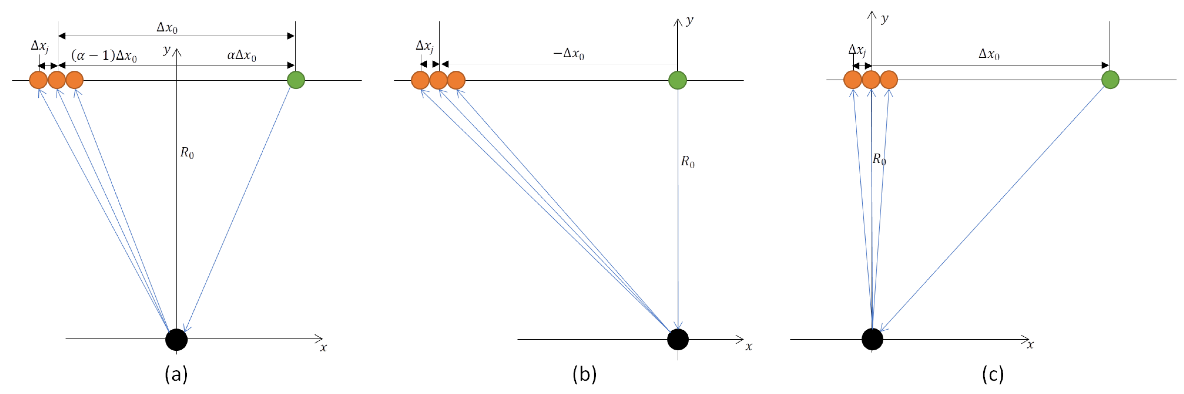
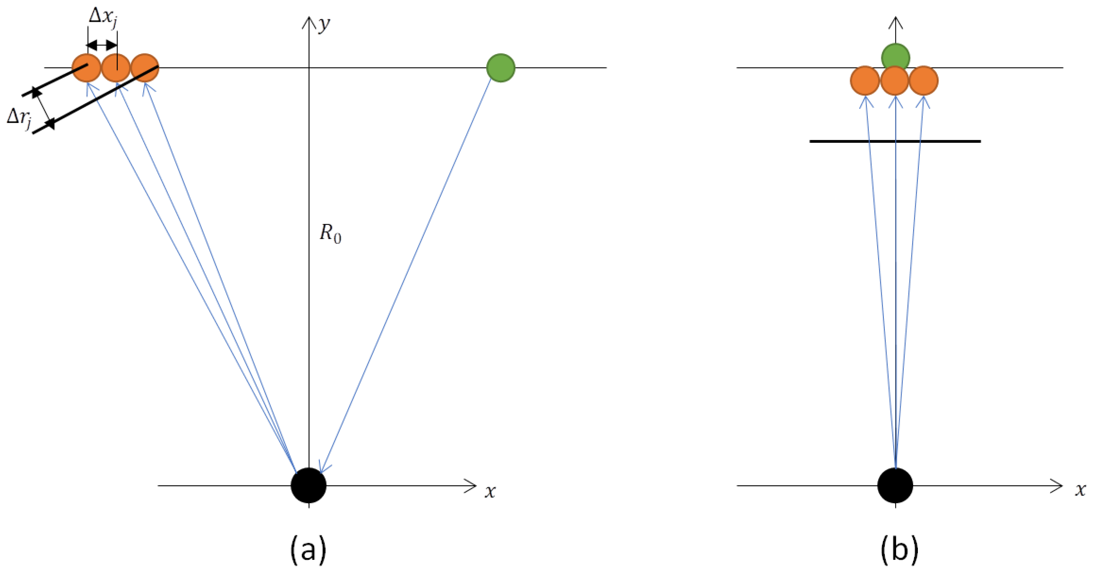
3.1. Geometry and General Hypotheses

In this section, we derive the formulation of the direct problem for the generic MAPS. We consider the simplified 1D geometry depicted in Figure 1. The transmitter (Tx) and the receiver (Rx) are assumed to move on the same straight orbit, over a flat Earth, with just a pure along-track separation (i.e., a time delay) between them. The justification for assuming this kind of simplified geometry is twofold: (i) it is in agreement with the past literature on the MAPS [1,8] giving a contribution in the same framework as the scientific literature on the MAPS; it eases the derivation of a closed expression for the LTI approach. It is worth noticing that the limits of the classic second-order approximation of the hodograph as in [11,12] are known. However, as mentioned in Section 3.2, the aim is also to demonstrate that this purely mathematical approach quickly becomes very complex: a semi-numerical approach is instead needed for bistatic geometries.

Under these hypotheses, and without losing in generality, we set the origin of the reference frame in the position corresponding to the maximum of the combined Tx and Rx patterns once projected on the ground. In turn, the origin of the reference frame can be associated with an ideal point target corresponding to the Doppler centroid of the acquisition and, around that point, we aim to solve the problem of multi-phase centers’ recombination.

The symbols that appear in Figure 1 have the following meaning:

• $R_0$ is the closest approach distance between the satellite and the center of the acquired swath. According to the previous hypotheses, $R_0$ is the same for both Tx and Rx satellites.
• $\Delta x_0$ is the along-track distance between the Tx and the Rx satellites. No hypothesis or constraint is assumed on its value that can even be of the same order of magnitude as the slant range $R_0$.
• $\Delta x_j$ is the along-track constant separation between the N receiving azimuth channels of the Rx satellite. Unlike $\Delta x_0$, $\Delta x_j$ is supposed to be much smaller than the slant range $R_0$. This is likely, since we deal with channels mounted on the same physical platform.
• $\alpha$ is a factor that defines the fraction of the along-track distance ($\Delta x_0$) that is between the Tx and the target placed at the origin of the reference frame. Then, $\left(1-\alpha \right)·\Delta x_0$ is the along-track distance between the Rx and the target.

The coordinates of the phase centers of the Tx, the jth Rx, the equivalent single channel Rx, and the target are, respectively:

$$\begin{array}{cc}\hfill Tx& =\left[\alpha ·\Delta x_0;R_0\right]\hfill \\ \hfill R{x}_j& =\left[-(1-\alpha )·\Delta x_0+\Delta x_j;R_0\right]\hfill \\ \hfill Rx& =\left[-(1-\alpha )·\Delta x_0;R_0\right]\hfill \\ \hfill P_T& =\left[0;0\right]\hfill \end{array}$$

(11)

The norm of the two-way distances as a function of the slow time t are:

$$\begin{array}{cc}\hfill R\left(t\right)=\sqrt{R_0^2+{\left(v_{s}t-\alpha ·\Delta x_0\right)}^2}+& \sqrt{R_0^2+{\left[v_{s}t-(\alpha -1)·\Delta x_0\right]}^2}\hfill \\ \hfill R_j\left(t\right)=\sqrt{R_0^2+{\left(v_{s}t-\alpha ·\Delta x_0\right)}^2}+& \sqrt{R_0^2+{\left[v_{s}t-(\alpha -1)·\Delta x_0+\Delta x_j\right]}^2}\hfill \end{array}$$

(12)

Equation (12) is also referred to as a $hodograph$ as it defines the distance as a function of time.

The objective of the MAPS in a generic geometry is still the same as for the monostatic approach [1,4,5,8,10], i.e., to re-create a non-aliased signal, sampled at $PR{F}_N=N·PR{F}_i$ starting from N aliased copies of the same signal, each sampled at $PR{F}_i$. The solution to this problem can be achieved:

• By interpreting the relation between the single-channel, non-aliased data and the multichannel, aliased data as a Linear, Time-Invariant (LTI) filter;
• By interpreting each frequency of the azimuth SAR data as the direction of arrival (DoA) of one useful signal (to be preserved), superimposed onto ($N-1$) ambiguities (to be canceled out).

The two approaches are explained in the following sections.

3.2. MAPS as an LTI Filter

Interpreting a multichannel acquisition as a bank of LTI filters is the most intuitive approach for those familiar with signal processing; it is the model explained in the publications on the monostatic MAPS [1,4,5,8,9,10].

3.2.1. Mathematical Modeling

We can also use the same approach resumed for the monostatic, zero Doppler case in Section 2.1 for the generalized MAPS problem depicted in Figure 1. Formally, the solution is in Equation (6), but now, we must handle bistatic signals with a Doppler centroid different from zero. Starting from Equation (5), it is convenient to make explicit the dependency of the functions on the two-way distance $R\left(t\right)$ from Equation (12):

$$\underset{H_{s,j}\left(f\right)}{\underbrace{FT\left\{exp\left(-\mathsf{ȷ}{\displaystyle \frac{2\pi }{\lambda }}·R_j\left(t\right)\right)\right\}}}=G_j\left(f\right)·\underset{H_s\left(f\right)}{\underbrace{FT\left\{exp\left(-\mathsf{ȷ}{\displaystyle \frac{2\pi }{\lambda }}·R\left(t\right)\right)\right\}}}$$

(13)

The formal definition of the direct transfer function is:

$$G_j\left(f\right)={\displaystyle \frac{FT\left\{exp\left(-\mathsf{ȷ}\frac{2\pi }{\lambda }·R_j\left(t\right)\right)\right\}}{FT\left\{exp\left(-\mathsf{ȷ}\frac{2\pi }{\lambda }·R\left(t\right)\right)\right\}}}={\displaystyle \frac{H_{s,j}\left(f\right)}{H_s\left(f\right)}}$$

(14)

where $\lambda$ is the wavelength of the carrier frequency of the SAR sensor.

From Equation (14) and Equation (12), it is evident that the key point when defining the direct function $G_j\left(f\right)$ lies in proper modeling of the hodographs and the FT of the exponentials whose argument depends on the hodographs. Although the numerical approach is always feasible, we prefer to come to the definition of closed equations. Actually, this approach is of some worth since it (i) gives continuity to the past studies on the MAPS, (ii) allows us to write the design matrix starting from the geometry of the acquisition and, (iii) shows how the complexity of the formulation increases when we get far from the SP-ZD condition.

Since the full mathematical derivation of the results is quite cumbersome, we focus on the general rationale rather than providing the step-by-step derivation of the solution in this paper.

We start from Equation (13). We must factorize the FT of the transfer function of the jth channel $H_{s,j}\left(f\right)$ into the product of two terms: (i) the one-channel response $H_s\left(f\right)$ that is now for a bistatic system and (ii) a term dependent on the shift $\Delta x_j$ of the azimuth channels on the Rx platform:

$$H_{s,j}\left(f\right)\approx \Delta H_{s,j}\left(f\right)·H_s\left(f\right)$$

(15)

Then, by plugging Equation (15) into Equation (13), we can simplify the common terms, coming to the following solution:

$$\begin{array}{cc}\hfill G_j\left(f\right)& ={\displaystyle \frac{H_{s,j}\left(f\right)}{H_s\left(f\right)}}\approx {\displaystyle \frac{\Delta H_{s,j}\left(f\right)·H_s\left(f\right)}{H_s\left(f\right)}}\hfill \\ & =\Delta H_{s,j}\left(f\right)\hfill \end{array}$$

(16)

Equation (16) defines the transfer function of the LTI filter that transforms the single-channel, bistatic acquisition into the jth-channel, bistatic acquisition. To compute the transfer function in Equation (16), the steps are as follows:

• Take Taylor’s series, up to the 2nd order and around the position corresponding to the Doppler centroid of the acquisition of the hodographs, for both the jth channel and the equivalent phase center of the single Rx channel after the MAPS;
• Take the FT of the polynomial approximation of the hodographs from the previous step;
• Linearize the FT of each of the N Rx channels;
• Factorize the linearized FT from the previous step into the two terms of Equation (15), to eventually isolate the response of the LTI filter from Equation (16).

The polynomial approximation of the hodograph, via Taylor’s series, is:

$$R_j\left(t\right)\approx \underset{C_{0,j}}{\underbrace{R_j\left(t_{0,j}\right)}}+\underset{A_{0,j}}{\underbrace{{\displaystyle \frac{d{R}_j\left(t\right)}{dt}}{|}_{t=t_{0,j}}}}·\left(t-t_{0,j}\right)+\underset{B{t}_{0,j}}{\underbrace{{\displaystyle \frac{1}{2}}{\displaystyle \frac{d^2{R}_j\left(t\right)}{d{t}^2}}{|}_{t=t_{0,j}}}}·{\left(t-t_{0,j}\right)}^2$$

(17)

where

• $t_0$ is the time corresponding to the Doppler centroid of the acquisition using the jth channel:

  $$t_{0,j}={\displaystyle \frac{\alpha \Delta x_j}{v_s}}$$

  (18)
• The first and the second derivative of the hodograph from Equation (12) are:

  $$\begin{array}{cc}\hfill {\displaystyle \frac{d{R}_0\left(t\right)}{dt}}=& {\displaystyle \frac{v_s·\left(v_{s}t-\alpha ·\Delta x_0\right)}{\sqrt{R_0^2+{\left(v_{s}t-\alpha ·\Delta x_0\right)}^2}}}+{\displaystyle \frac{v_s·\left(v_{s}t-(\alpha -1)·\Delta x_0\right)}{\sqrt{R_0^2+{\left(v_{s}t-(\alpha -1)·\Delta x_0\right)}^2}}}\hfill \\ \hfill {\displaystyle \frac{d^2{R}_0\left(t\right)}{d{t}^2}}=& {\displaystyle \frac{v_s^2}{\sqrt{R_0^2+{\left(v_{s}t-\alpha ·\Delta x_0\right)}^2}}}·\left[1-{\displaystyle \frac{v_s^2{t}^2}{\sqrt{R_0^2+{\left(v_{s}t-\alpha ·\Delta x_0\right)}^2}}}\right]+\hfill \\ \hfill & {\displaystyle \frac{v_s^2}{\sqrt{R_0^2+{\left(v_{s}t-(\alpha -1)·\Delta x_0\right)}^2}}}·\left[1-{\displaystyle \frac{v_s^2{t}^2}{\sqrt{R_0^2+{\left(v_{s}t-(\alpha -1)·\Delta x_0\right)}^2}}}\right]\hfill \end{array}$$

  (19)

Then, Equation (12) can be approximated as:

$$\begin{array}{cc}\hfill R\left(t\right)& \approx C_{0,0}+A_{0,0}·\left(t-t_{0,0}\right)+B_{0,0}·{\left(t-t_{0,0}\right)}^2\hfill \\ \hfill R_j{\left(t\right)}_{0,j}& \approx C_{0,j}+A_{0,j}·\left(t-t_{0,j}\right)+B_{0,j}·{\left(t-t_{0,j}\right)}^2\hfill \end{array}$$

(20)

Before continuing with the derivation of the LTI filter in the frequency domain, the results from Equations (17) and (20) deserve further consideration. The approximation to the second order of the hodograph is the same as that used for the SP-ZD case. It is possible to include higher-order terms in the polynomial approximation, but we chose to stop to the second order to have the chance of computing the closed mathematical expression of the Fourier transform of the approximated hodograph. Another aspect is that for the SP-ZD case, both Equations (17) and (20) have the linear term equal to zero. It is intuitive since in that case, the approximation of the hodograph is around its vertex and therefore, the first derivative is equal to zero. In the generalized bistatic MAPS, the first-order term can be different from zero since we removed the constraint of zero Doppler acquisition.

The FT of the transfer function for the equivalent single-channel acquisition after the MAPS (see $H_s\left(f\right)$ in Equations (13) and (16) can be computed in closed form by recalling the known FT of the Gaussian function and can be written as:

$$\begin{array}{cc}\hfill H_s\left(f\right)\propto & exp\left\{-j{\displaystyle \frac{2\pi }{\lambda }}{C}_{0,0}\right\}·\hfill \\ \hfill & exp\left\{j{\displaystyle \frac{\pi }{2\lambda }}{\displaystyle \frac{A_{0,0}^2}{B_{0,0}}}\right\}·\hfill \\ \hfill & exp\left\{-j\pi {\displaystyle \frac{A_{0,0}}{B_{0,0}}}f\right\}·\hfill \\ \hfill & exp\left\{-j{\displaystyle \frac{\pi \lambda }{2}}{\displaystyle \frac{1}{B_{0,0}}}{f}^2\right\}·\hfill \\ \hfill & exp\left\{-j2\pi f{t}_{0,0}\right\}\hfill \end{array}$$

(21)

The FT of the transfer function of each channel $H_{s,j}\left(f\right)$ is formally identical to Equation (21) but with the argument of the exponential functions computed according to the proper $t_{0,j}$ from Equation (18) corresponding to the $j^{th}$ channel. This is a non-trivial difference, and a consequence is that $H_s\left(f\right)$ and $H_{s,j}\left(f\right)$ do not differ only in an extra linear phase but also in the coefficients themselves.

This makes it more complex to recognize in $H_{s,j}\left(f\right)$ the expression of $H_s\left(f\right)$. As a consequence, to identify the transfer function $\Delta H_{s,j}\left(f\right)$ from Equation (16), we operated an approximation to the first order of the argument of the exponential in $H_{s,j}\left(f\right)$ aimed at writing them in the following form:

$$\begin{array}{cc}\hfill C_{0,j}& \approx C_{0,0}+\Delta C_{0,j}\hfill \\ \hfill {\displaystyle \frac{A_{0,j}^2}{B_{0,j}}}& \approx {\displaystyle \frac{A_{0,0}^2}{B_{0,0}}}+\Delta {\displaystyle \frac{A_{0,j}^2}{B_{0,j}}}\hfill \\ \hfill {\displaystyle \frac{A_{0,j}}{B_{0,j}}}& \approx {\displaystyle \frac{A_{0,0}}{B_{0,0}}}+\Delta {\displaystyle \frac{A_{0,j}}{B_{0,j}}}\hfill \\ \hfill {\displaystyle \frac{1}{B_{0,j}}}& \approx {\displaystyle \frac{1}{B_{0,0}}}+\Delta {\displaystyle \frac{1}{B_{0,j}}}\hfill \\ \hfill t_{0,j}& =t_{0,0}+\Delta t_{0,j}\hfill \end{array}$$

(22)

The expression of $\Delta H_{s,j}\left(f\right)$ can be approximated as:

$$\begin{array}{cc}\hfill H_{s,j}\left(f\right)\approx & exp\left\{-j{\displaystyle \frac{2\pi }{\lambda }}\Delta C_{0,j}\right\}·\hfill \\ \hfill & exp\left\{j{\displaystyle \frac{\pi }{2\lambda }}\Delta {\displaystyle \frac{A_{0,j}^2}{B_{0,j}}}\right\}·\hfill \\ \hfill & exp\left\{-j\pi \Delta {\displaystyle \frac{A_{0,j}}{B_{0,j}}}f\right\}·\hfill \\ \hfill & exp\left\{-j{\displaystyle \frac{\pi \lambda }{2}}\Delta {\displaystyle \frac{1}{B_{0,j}}}{f}^2\right\}·\hfill \\ \hfill & exp\left\{-j2\pi f\Delta t_{0,j}\right\}\hfill \end{array}$$

(23)

As previously mentioned, Equation (23) was derived under the simplified hypotheses stated in Section 3, and its effectiveness is assessed in Section 4.1 using a conveniently developed simulator. Again, we remark that the application of LTI-MAPS to a real-world scenario (i.e., with Keplerian orbits and an ellipsoidal Earth) would necessarily require switching to a semi-numerical approach, which we also investigated but did not include here since it was beyond the scope and the objectives of the current paper. Equation (23) is to the generalized MAPS as Equation (6) is to the monostatic MAPS. It means that we can use Equation (23) to create the proper design matrix for each Doppler frequency to be inverted [5]. Now that the zero Doppler hypothesis has been removed, the frequency axis is centered around the actual Doppler frequency of the acquisition. This is consistent with the choice of the point where the hodographs were linearized.

3.2.2. Processing Scheme

Here, we propose an in-principle workflow to process data from N azimuth channels to re-create a single data point with a PRF that is N times the one from the acquisition. Since in this section, we are handling MAPS recombination as a bank of LTI filters, it is straightforward to extend the processing for the SP-ZD MAPS [1,4,8] to the current bistatic generalized case. The processing scheme, whose block diagram is in Figure 2, is the same as that proposed in [5], whose main steps are as follows:

• Calculate a double Fourier transform of each receiving dataset and concatenate them in an $NK\times P$ (where P is the number of samples along range) matrix $S_{Tot}$;
• Make a loop on the Doppler frequency bins and for each Doppler frequency (i.e., $f\left(k\right)$ with $k=1,\dots ,K$), extract the samples corresponding to the multiples of PRF (i.e., $f\left(k\right)+n·PRF=f(k+n·K)$) of both data ${\underline{\underline{S}}}_k$ and recombination matrix ${\underline{\underline{G}}}_k$.
• Determine the pseudo-inversion of the matrix ${\underline{\underline{G}}}_k$ to estimate the spectrum of the data corresponding to the current Doppler frequency bins, i.e., ${\underline{\underline{D}}}_k$

By iterating on the previous steps for all the Doppler frequencies, we obtain the estimation of the target spectrum over a Doppler frequency interval whose extension is $N·PRF$, as expected. The resulting matrix $\underline{\underline{\widehat{D}}}$ is the 2D-FT range-compressed equivalent bistatic data. It is then 2D inverse Fourier transformed and focused as canonical single-channel bistatic data to obtain the reconstructed reflectivity map in the SAR domain (i.e., SLC image). Finally, since we approximated the hodograph around the position corresponding to the Doppler centroid of the acquisition, any azimuth demodulation of the data before the recombination is unnecessary.

3.3. MAPS as DoA

It is well known from SAR theory [13] that an echo impinging on the SAR antenna with a squint angle $\psi$ has a Doppler frequency f defined as:

$$\begin{array}{cc}\hfill f& =-{\displaystyle \frac{1}{\lambda }}·\left({\overrightarrow{u}}_{Tx/P_t}·{\overrightarrow{v}}_{s,Tx}+{\overrightarrow{u}}_{Rx/P_t}·{\overrightarrow{v}}_{s,Rx}\right)\hfill \\ \hfill & =-{\displaystyle \frac{v_s}{\lambda }}·\left(sin{\psi }_{Tx}+sin{\psi }_{Rx}\right)\hfill \\ \hfill & =-{\displaystyle \frac{2v_s}{\lambda }}·sin{\psi }_{Eq}\hfill \end{array}$$

(24)

In the previous equations:

• ${\overrightarrow{u}}_{Tx/P_t}$ and ${\overrightarrow{u}}_{Tx/P_t}$ are the unit vectors from the point target to the Tx and Rx sensors, respectively;
• The squint angles ${\psi }_{Tx}$ and ${\psi }_{Rx}$ are defined with respect to the zero Doppler direction of each sensor and the convention is that negative squint angles are for forward-looking sensors (thus generating a positive Doppler frequency).

Conversely, given a Doppler frequency f, infinite DoAs, corresponding to integer multiples of the PRF, are superimposed: SAR is inherently ambiguous along azimuth, because of its Pulse Repetition Frequency (PRF). We can write that

$$\begin{array}{cc}\hfill f& \equiv f+k·PRF\hfill \\ \hfill S\left(f\right)& =\sum _{k=-\infty }^{+\infty }\widehat{S}\left(f+k·PRF\right)\hfill \end{array}$$

(25)

where $\widehat{S}\left(f\right)$ is the non-ambiguous version of the acquired ambiguous signal $S\left(f\right)$.

Dealing with the MAPS architecture, the echo is recorded by N sensors so that N delayed copies of the same signal are recorded. Given a Doppler frequency and knowing the DoA of the signal and the $N-1$ DoAs of interference, we can compute the N coefficients of the optimum recombination filter that would maximize the signal and minimize the ambiguities. Many beamformers have been studied [14,15]. Here, we use the Minimum Variance Distortionless Reconstruction (MVDR) approach, also known as Capon’s beamformer [16]. MVDR has the significant advantage for SAR applications of minimizing the overall error of the reconstructed signal with the constraint of preserving the wanted signal. Please note that this approach is of great value as it can also control the noise in the reconstructed signal. Other beamforming techniques (e.g., null-steering) can obtain better results in rejecting the interference. However, they may suffer from excessive noise magnification, thus vanishing the advantage of the MAPS on the SNR. Eventually, with N data, only $N-1$ ambiguous signals can be attenuated since one degree of freedom is spent to preserve the nominal signal.

We define the vector of the signals, recorded by the N receivers, coming from the nominal direction $\psi$ and from its ambiguous directions ${\psi }_{amb}$ as:

$$\begin{array}{cc}\hfill \underline{t}& ={\left[\begin{array}{ccccc}exp\left(-\mathsf{ȷ}{\displaystyle \frac{2\pi }{\lambda }}\Delta x_{1}sin\psi \right)& \dots & exp\left(-\mathsf{ȷ}{\displaystyle \frac{2\pi }{\lambda }}\Delta x_{j}sin\psi \right)& \dots & exp\left(-\mathsf{ȷ}{\displaystyle \frac{2\pi }{\lambda }}\Delta x_{N}sin\psi \right)\end{array}\right]}^T\hfill \\ \hfill {\underline{t}}_{amb}& ={\left[\begin{array}{ccccc}exp\left(-\mathsf{ȷ}{\displaystyle \frac{2\pi }{\lambda }}\Delta x_{1}sin{\psi }_{amb}\right)& \dots & exp\left(-\mathsf{ȷ}{\displaystyle \frac{2\pi }{\lambda }}\Delta x_{j}sin{\psi }_{amb}\right)& \dots & exp\left(-\mathsf{ȷ}{\displaystyle \frac{2\pi }{\lambda }}\Delta x_{N}sin{\psi }_{amb}\right)\end{array}\right]}^T\hfill \end{array}$$

(26)

where the relation between the nominal DoA and its ambiguities is from Equation (25):

$$sin\psi =-{\displaystyle \frac{\lambda }{2v_s}}·f\Rightarrow sin{\psi }_{amb}=-{\displaystyle \frac{\lambda }{2v_s}}·(f+k·PRF)$$

(27)

The coefficients of Capon’s beamforming are computed according to the following known solution [16,17]:

$$\underline{w}={\displaystyle \frac{{\underline{\underline{R}}}_t^{-1}\underline{a}}{{\underline{a}}^H{\underline{\underline{R}}}_t^{-1}\underline{a}}}$$

(28)

Focusing on the MAPS case, the vector $\underline{w}$ provides a set of N coefficients for each of the M frequency bins (i.e., the ones where the FT of the data is computed) in the interval $I=\left[\lceil -N/2\rceil ·PRF;\lfloor -N/2\rfloor ·PRF\right]$. Then, for each Doppler frequency $f\in I$, the terms in Equation (28) are as follows:

• ${\underline{\underline{R}}}_t$ is the covariance matrix of the observations. In practical cases, the sampled correlation matrix is used instead, i.e., ${\underline{\underline{\widehat{R}}}}_t$ is the $N\times N$ squared matrix defined as the sum of K DoAs corresponding to the nominal frequency f:

  $${\underline{\underline{\widehat{R}}}}_t=\sum _{k=-K/2}^{+K/2}{\underline{t}}_k{\underline{t}}_k^H$$

  (29)
  K is a generic number that, according to Equation (25), goes to ∞. In practice, it is limited by the number N of azimuth channels, and increasing K over N does not bring advantages. When $k=0$, there is the useful signal.
• $\underline{a}$ is the vector of the main signal’s DoA. It is formally equal to the first line in Equation (26), where $sin\psi$ is computed according to the current Doppler frequency.

By juxtaposing the coefficients $\underline{w}$ for each Doppler frequency $f\in I$, we obtain the matrix $\underline{\underline{W}}$ representing the full set of coefficients to be used for MAPS reconstruction. Again, for the actual implementation of the MAPS as a Doppler frequency-dependent filter, we can refer to the clear and intuitive description in [5].

Two aspects deserve particular attention when implementing MVDR for generic bistatic and non-zero Doppler SAR. We address them in the following sections.

3.3.1. Extra Phase Compensation

When Tx and Rx are physically separated, it is necessary to compensate for the extra phase that exists between the channels. To analyze the problem, we can refer to Figure 3.

In Figure 3, we represent the geometry for two zero Doppler acquisitions: the panel on the left represents the typical monostatic geometry whilst the one on the right is for a bistatic case. Although the two cases have the same Doppler centroid, the bistatic multichannel acquisition shows an extra phase term between the channels that are not there for the monostatic case. This phase term depends on the geometry only and according to Figure 3, we can write:

$$\begin{array}{cc}\hfill & \Delta r_j=\Delta x_{j}sin{\psi }_{Rx}\hfill \\ \hfill & \Delta {\varphi }_j=-{\displaystyle \frac{2\pi }{\lambda }}\Delta r_j=-{\displaystyle \frac{2\pi }{\lambda }}\Delta x_{j}sin{\psi }_{Rx}\hfill \end{array}$$

(30)

The result from Equation (30) is subtracted from the data of each of the N receiving channels (see Equation (4)) before performing the MAPS recombination, i.e.,

$${\widehat{s}}_j\left(t\right)=s_j\left(t\right)·e^{-j\Delta {\varphi }_j}.$$

(31)

3.3.2. Frequency-to-DoA Conversion in Bistatic Geometry

The objective of this subsection is to accurately compute the DoA of an echo whose Doppler frequency f is known. To achieve this result, we start from Equation (24), which defines the relation between the squint angles ${\psi }_{Tx}$, ${\psi }_{Rx}$ and the Doppler frequency f, to find the exact point on the Earth’s surface that generates the echo with a given delay and Doppler. This is the well-known problem of direct SAR geocoding [18,19], where the point on the Earth’s surface is obtained as the solution of the system composed by the following three equations: (i) the Doppler frequency equation, (ii) the time delay, and (iii) the geoid surface. This paper deals with the simplified 2D geometry presented in Section 3.1; thus, the canonical geolocation system of equations simplifies into just one equation. Starting from Equation (24), and making explicit the dependency of squint angles ${\psi }_{Tx}$, ${\psi }_{Rx}$ on the ground position $x_p\left(f\right)$ that is generating the Doppler frequency f, we can write:

$$\begin{array}{cc}\hfill f& =-{\displaystyle \frac{v_s}{\lambda }}·\left(sin{\psi }_{Tx}+sin{\psi }_{Rx}\right)\hfill \\ \hfill & =-{\displaystyle \frac{v_s}{\lambda }}·\left\{{\displaystyle \frac{x_p-\alpha \Delta x_0}{\sqrt{{\left(x_p-\alpha \Delta x_0\right)}^2+R_0^2}}}+{\displaystyle \frac{x_p-\left(\alpha -1\right)\Delta x_0}{\sqrt{{\left[x_p-\left(\alpha -1\right)\Delta x_0\right]}^2+R_0^2}}}\right\}\hfill \end{array}$$

(32)

It is worth remarking that from a practical point of view, here, the observables of the problem are the SAR data as a function of the Doppler frequency f. Still, we have no direct access to the parameter of the model, i.e., the on-ground position $x_p$. In other words, we know the Doppler frequency, but we do not know the position of the target generating that Doppler. It is an inverse problem that requires solving Equation (32) for each Doppler frequency to eventually obtain the position $x_p\left(f\right)$ as the solution. Moreover, contrary to the canonical monostatic geometry, the position of the equivalent phase center corresponding to each Doppler frequency migrates over the trajectory and does not correspond to the midposition between Tx and Rx. From the solution of Equation (32), $x_P$ is known. Then, the squint angles are:

$$\begin{array}{cc}\hfill {\psi }_{Tx}& =arctan\left({\displaystyle \frac{\alpha \Delta x_0-x_p\left(f\right)}{R_0}}\right)\hfill \\ \hfill {\psi }_{Rx}& =arctan\left({\displaystyle \frac{(\alpha -1)\Delta x_0-x_p\left(f\right)}{R_0}}\right)\hfill \end{array}$$

(33)

The Doppler frequency can be evaluated using Equation (24). However, Equation (24) can be inverted to compute an equivalent squint angle ${\psi }_{Eq}$ that is the corresponding DoA. From this, the ground-pointing $x_{p,Eq}\left(f\right)$ which generates the echo can be found:

$$\begin{array}{cc}\hfill {\psi }_{Eq}& =-arcsin{\displaystyle \frac{\lambda f}{2v_s}}\hfill \\ \hfill x_{p,Eq}\left(f\right)& =R_{0}tan{\psi }_{Eq}\hfill \end{array}$$

(34)

Then, the spatial shift with respect to the locus of the Doppler centroid is:

$$\Delta x_{p,Eq}\left(f\right)=x_{p,Eq}\left(f\right)\left(f_{DC}\right)-x_{p,Eq}\left(f\right)$$

(35)

Eventually, the bistatic phase center migration is:

$$\Delta Az\left(f\right)=\Delta x_{p,Eq}\left(f\right)-x_p\left(f\right)$$

(36)

The angles in the DoA vectors in Equation (26) must be computed considering the correction term in Equation (36) applied to the solution $x_p\left(f\right)$.

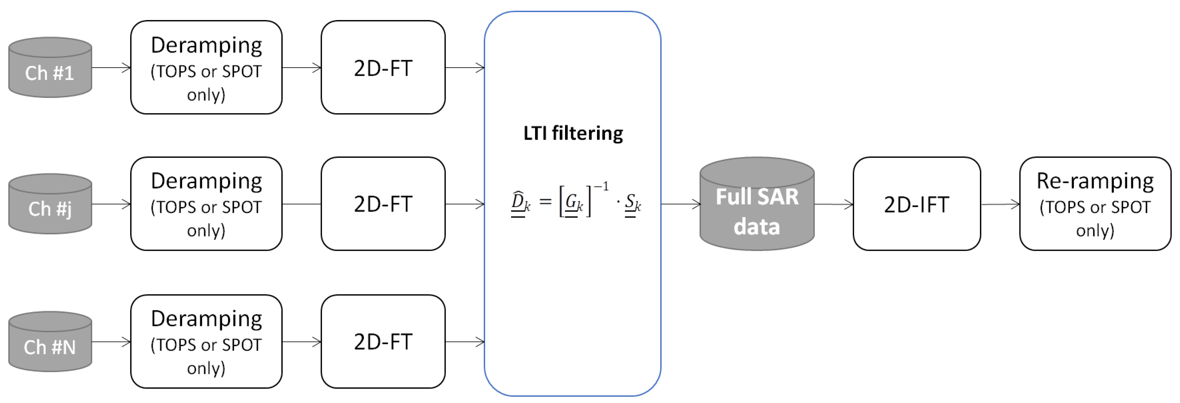
3.3.3. Processing Scheme

Figure 4 reports the flow chart that depicts the principle of a processing chain for MVDR-MAPS. The main steps are:

• The data from each receive channel are compensated for the phase term defined in Equation (30);
• In case of TOPS or SPOT acquisitions, deramping is applied;
• The Doppler spectrum is demodulated (i.e., centered) in the base-band interval;
• Data are transformed in the Doppler domain;
• MVDR coefficients from Equation (28) are applied to make the reconstruction;
• MAPS-recombined data go through the inverse operations of steps (4), (3), and (2), i.e., Az-IFT, azimuth modulation to nominal Doppler centroid, and re-ramping.

The output data are sampled at a frequency that is N times the acquisition: $PR{F}_i$. Although the processing works on the demodulated data, around zero Doppler, the vectors of DoAs used in Equation (28) are computed according to the nominal frequency domain of the signal. This is necessary because of the non-linear transformation between frequency and angles (see Equation (24)).

4. Simulation Results for Bistatic MAPS

In the current section, we present the results of a bistatic MAPS experiment obtained using an end-to-end simulator up to the focused recombined data. We set up a 1D (azimuth-only) end-to-end simulator for the N MAPS channels in a generic bistatic geometry but with the simplified geometry presented in Figure 1, i.e., a flat Earth and straight satellite trajectory. Despite these simplifications, the simulated data were fully suitable for proving the effectiveness of the reconstruction methods presented in the previous sections, as the simulated 1D data inherently contained both signal and azimuth ambiguities (the one to be solved). Thus, limiting the simulations to azimuth only (i) still preserved the characteristics of the data we were interested in and (ii) did not undermine the validity of the following results. The simulated SAR data were then recombined, according to the two approaches previously presented (i.e., LTI and MVDR), and their performance in improving the ambiguity rejection were compared. The main goal of the analysis was to assess the effectiveness and the limitations of the two MAPS approaches we presented. Consequently, we considered the First Ambiguity Azimuth Point Target Ambiguity (to signal) Ratio (FAAzPTAR ) as the figure of merit ancillary to this aim. The FAAzPTAR (whose expression is in Equation (37)) is defined as the canonical AzPTAR but it refers to the first left and right ambiguities only, i.e., the ones that a three-channel MAPS can mitigate by reconstruction:

$$FAAzPTAR={\displaystyle \frac{P_{Amb1}}{P_t}}={\displaystyle \frac{{\left[{\int }_{-PRF-\frac{B_{Az}}{2}}^{-PRF+\frac{B_{Az}}{2}}S\left(f\right)df\right]}^2+{\left[{\int }_{PRF-\frac{B_{Az}}{2}}^{PRF+\frac{B_{Az}}{2}}S\left(f\right)df\right]}^2}{2·{\left[{\int }_{-\frac{B_{Az}}{2}}^{\frac{+B_{Az}}{2}}S\left(f\right)df\right]}^2}}$$

(37)

The main parameters of the system we considered for our simulations are in

Table 1. SAR system simulation.

Parameter	Symbol	Value	UoM
Slant range zero Doppler	$R_0$	650.0	km
Satellite velocity	$v_s$	7500.0	m/s
Antenna length	$L_a$	11.0	m
Number of MAPS channels	N	3	-
Pulse rep. freq.	$PRF$	1365.4	Hz
Tx-Rx distance	$\Delta x_0$	$\left[0,400\right]$	km
Normalized bistatic Doppler centroid	$\alpha$	$\left[0,1\right]$	-
Target Doppler bandwidth	$B_{Az}$	$PRF$	Hz
Acquisition mode	-	Stripmap	-

. Please note that (i) the values we chose were plausible for a real instrument, even if they did not refer to any existing or under-development instrument, and (ii) the PRF of the instrument was the one that led to a uniform sampling [1]:

$$PR{F}_{Uni}={\displaystyle \frac{2v_s}{N·\Delta x_j}}$$

(38)

where the value of the inter-channel distance $\Delta x_j$ is from the parameters in Table 1; hence, $\Delta x_j=3.67$ m.

Furthermore, starting from the instrument configuration and geometry in Table 1, we used the same parameters with two different carrier frequencies: L-band ($1.275$ GHz) and C-band ($5.405$ GHz). This choice stresses the dependency of the recombination on the wavelength that is expected to be one of the key parameters since the MAPS is essentially based on pure-phase filters: the shorter the wavelength, the more sensitive the phase.

In the following, Section 4.1 reports the results for the LTI approach (Section 3.2); Section 4.2 refers to MVDR (Section 3.3). We also compare the results of the two approaches highlighting their advantages and pitfalls.

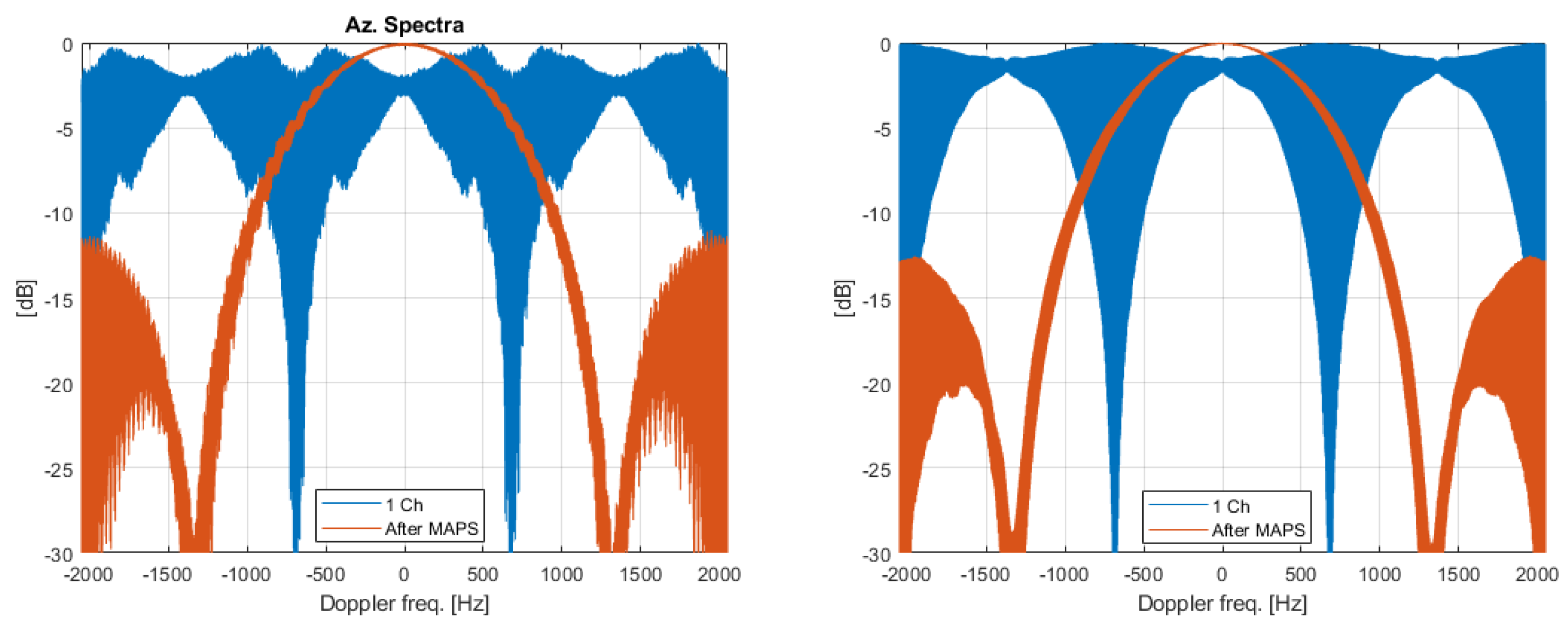
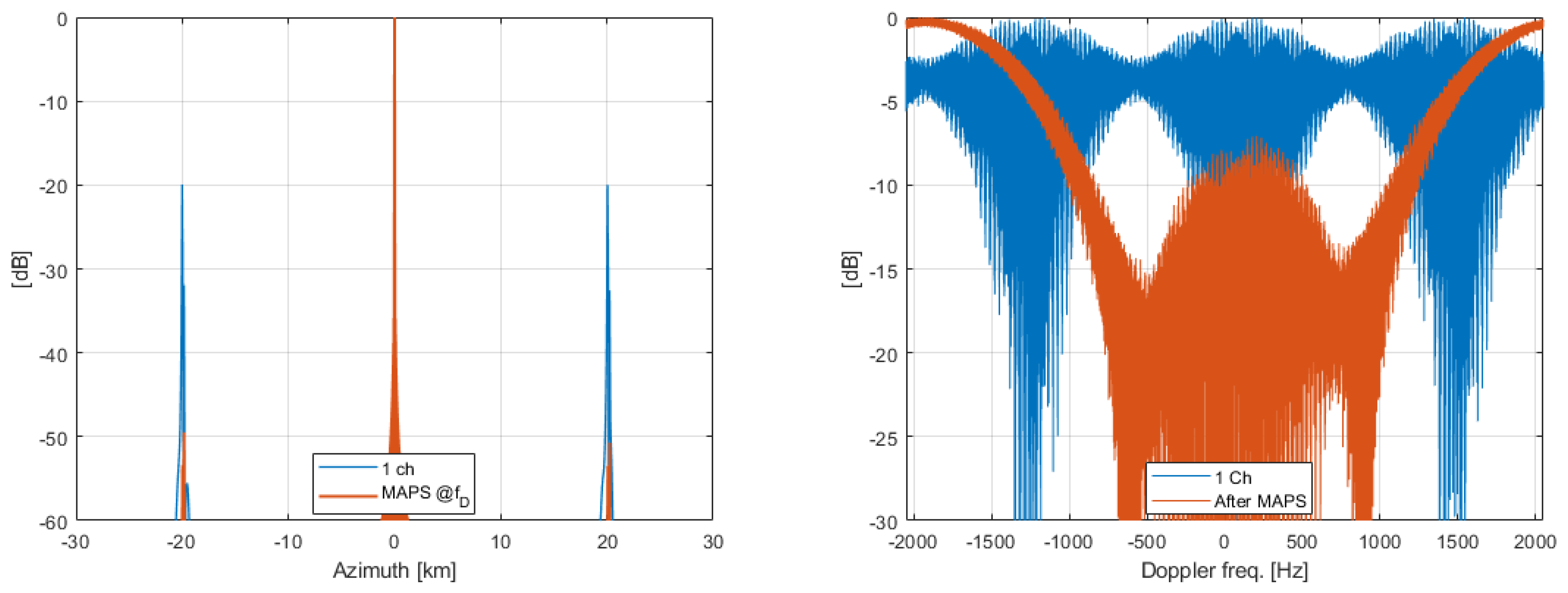
4.1. Results for MAPS as LTI Filter

In this paragraph, we present and discuss the experimental results obtained by implementing MAPS digital beamforming as the inversion of an LTI filter (see Section 3.2). The improvement in the FAAzPTAR after a bistatic MAPS is depicted in Figure 5 for the L-band system (left panel) and the C-band system (right panel) as a function of the Tx-Rx distance $\Delta x_0$ (y-axis) and the corresponding normalized bistatic Doppler centroid $\alpha$ (x-axis).

Regardless of the carrier frequency of the SAR, we observe that the MAPS strongly attenuates the first ambiguity, with a gain on the FAAzPTAR close to 50 dB, when the LTI filters are written around the bistatic zero Doppler. This condition is achieved when the Tx and Rx antennas are pointing halfway, one forward and the other backward, and it corresponds to $\alpha =0.5$ along the x-axis. Furthermore, the effectiveness of the MAPS on bistatic zero Doppler acquisitions is insensitive to the distance between Tx and rx ($\Delta x_0$ along the y-axis), i.e., we can see the yellow “vertical line” in both the panels of Figure 5. An example of IRF is reported in Figure 6.

Conversely, from Figure 5 we can observe that the shape and the extension of the yellowish area (which is the condition where the MAPS is effective) are different for the L-band (left panel) and C-band (right panel). This behavior is justified because implementing the MAPS as a bank of LTI filters relies on Taylor’s series of the hodograph around the locus corresponding to the Doppler centroid of the acquisition. Then, the error obtained by taking the approximation of the hodograph is magnified on the phase of the SAR signal since it is scaled by the reciprocal of the wavelength (i.e., ${\displaystyle \frac{2\pi }{\lambda }}$): the higher the carrier frequency, the shorter the wavelength, and the bigger the phase error. Then, it is expected that the MAPS as an LTI filter would perform worse in the C-band than in the L-band. In particular, the advantage from the MAPS almost nullifies in the C-band for (i) a Tx-Rx separation larger than 300 km, and (ii) when pointing far from the bistatic zero Doppler. In the same conditions, a small gain (around 5 dB) is still present for the L-band case: Figure 7 reports the IRF and the Doppler spectrum for an L-band system with $\alpha =1$ and $\Delta x_0=400$ km.

4.2. Results for MAPS as DoA Estimation

In this paragraph, we present the results of the same sensitivity analysis as in Section 4.1 but obtained by implementing MAPS digital beamforming as a DoA estimation (see Section 3.3). Similarly to Figure 5, Figure 8 depicts the improvement in the FAAzPTAR after the bistatic MAPS with respect to the value from each of the three channels as a function of the Tx-Rx distance $\Delta x_0$ (y-axis) and the corresponding normalized bistatic Doppler centroid $\alpha$ (x-axis).

We can make similar considerations for the DoA as for the LTI approach, i.e., the MAPS is very effective around bistatic zero Doppler but its capability to attenuate the azimuth ambiguity degrades when (i) the Tx−Rx separation is larger than 300 km, and (ii) the bistatic Doppler centroid gets far from the zero. Despite this, we can observe some peculiarities of the DoA implementation, i.e.,

• The yellowish area in Figure 8 is greater than in Figure 5. This means that the DoA approach is able to perform better than the LTI approach in a wider variety of cases.
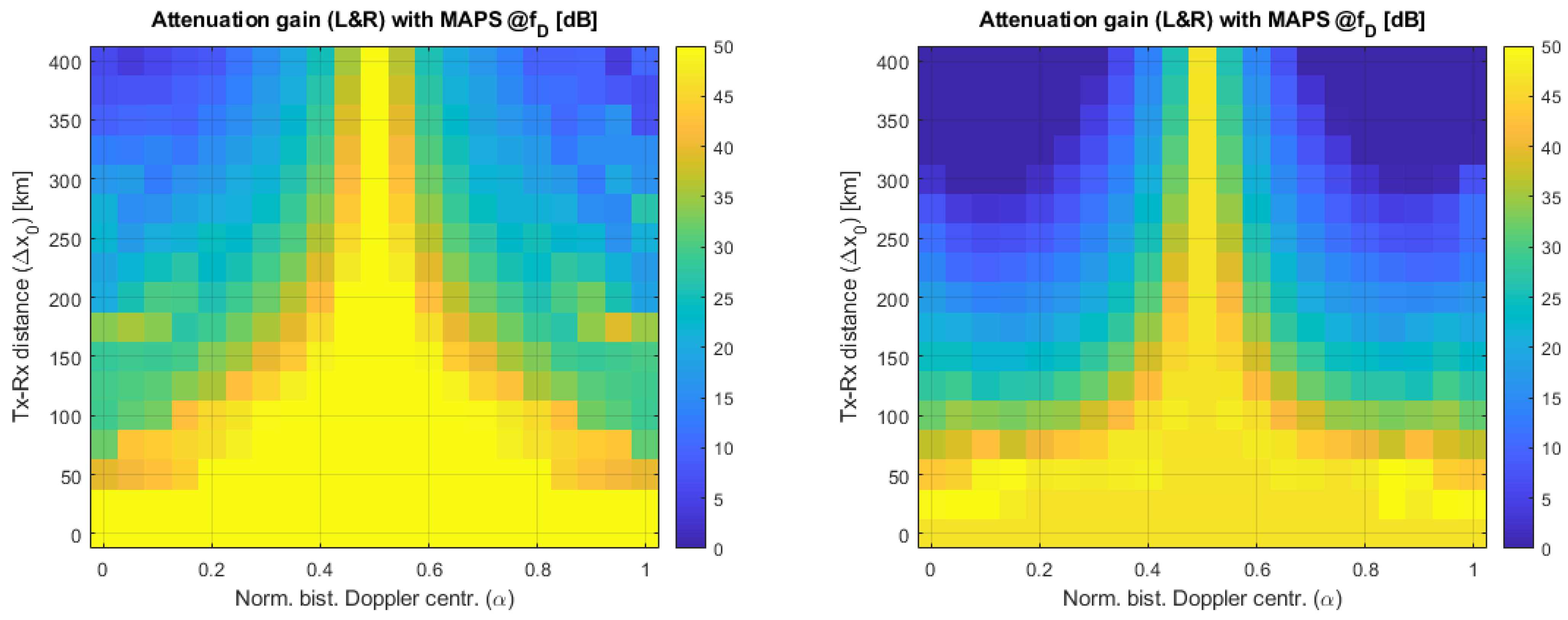
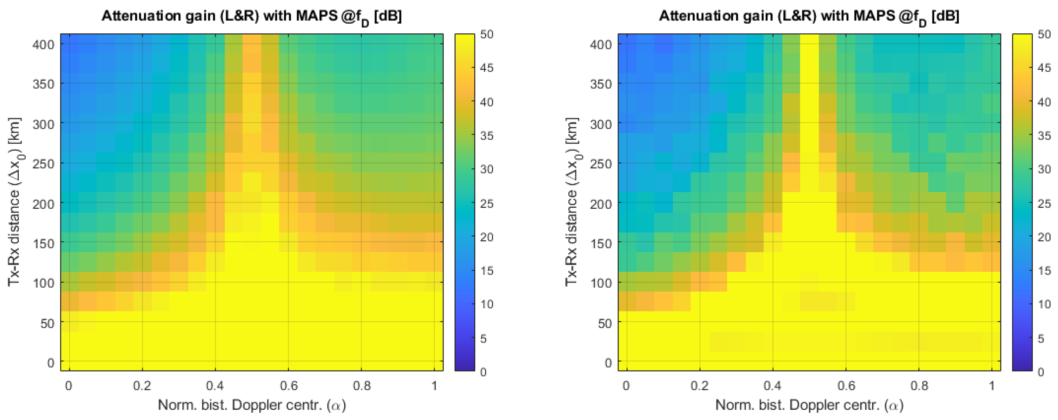
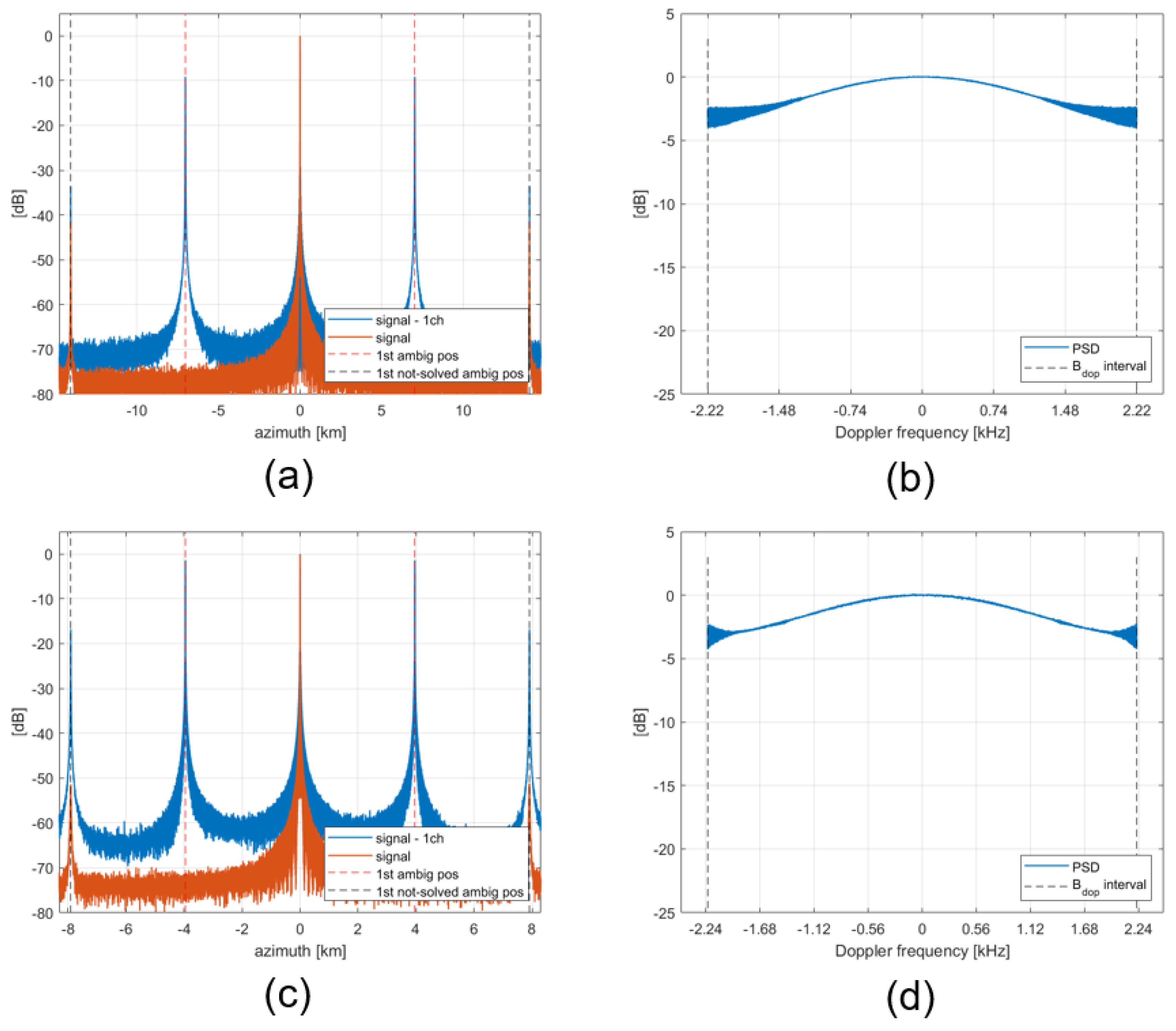
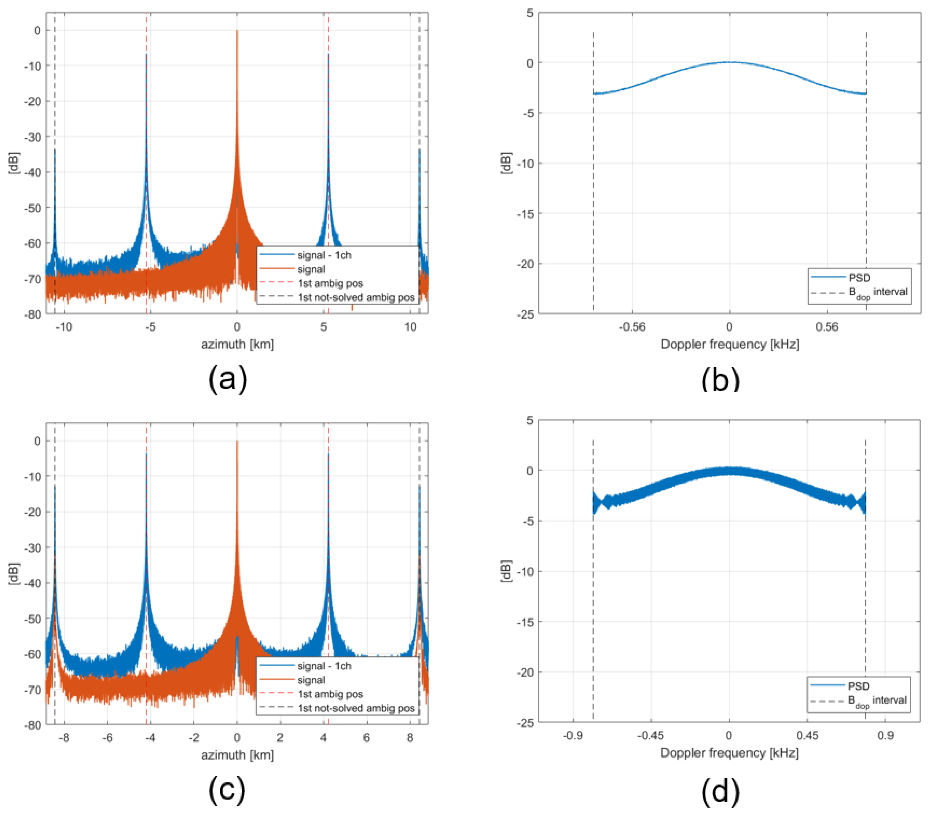
• The gain on FAAzPTAR is almost insensitive to the carrier frequency. The left and right panels of Figure 8 are fully comparable in terms of colors.
• The gain on FAAzPTAR does not nullify for extreme geometries (large Tx-Rx distances and Doppler centroid far from zero) but a significant gain on the FAAzPTAR is feasible (e.g., about 30 dB for $\alpha =1;\Delta x_0=400$ km).

An in-depth analysis of the reasons why the DoA-based MAPS does not achieve the perfect cancellation of ambiguities for all the cases is beyond the scope of the present work and shall deserve further investigations in the future. However, an intuitive justification is here provided. MVDR, as many other DoA algorithms [14,15], is based on the hypothesis that the exact covariance matrix is known. However, as underlined in Section 3.3, Equation (29), we deal with an estimation of the exact covariance matrix. Another limitation is the limited number of azimuth-receiving channels that contrasts with the potential necessity of canceling an infinite number of interfering directions. This sub-optimal condition results in sub-optimal results, especially for those cases with an acquisition geometry far from the zero Doppler condition and a worse estimation of the covariance matrix.

Despite this, in practical cases, the gain on FAAzPTAR in Figure 8 is a relevant result that can strongly improve the overall AzPTAR for SLC products as well as the performance of higher-level applications, e.g., interferometry [20] and Doppler anomaly estimation [21,22]. To give a concrete result of what this means on the IRF, we can refer to Figure 9 where we report the results of the end-to-end simulator for the L-band system when assuming $\Delta x_0=400$ km and $\alpha =1$. Contrary to Figure 7, in Figure 9, we notice the gain in abating the level of the first azimuth ambiguities (left panel) and consequently, the Doppler spectrum (right panel) is significantly better when MVDR is used. Furthermore, the gain in canceling the ambiguities is in line with (or even better than) post-processing algorithms for local ambiguity cancellation [23,24,25] but with the advantages, for the DoA-based MAPS, of operating (i) on RGC data, and not at the application level as, e.g., interferograms, and (ii) on the whole image (not locally). Then, it is possible to deliver SLC images with homogeneously improved AASR performance and a fully preserved Doppler spectrum.

We also observe that the results in Figure 8 show a slight asymmetry of the FAAzPTAR gain. It is better if the direction of arrival corresponds to the zero Doppler of the receiver, i.e., $\alpha =1$, than to the zero Doppler of the transmitter, i.e., $\alpha =0$; the gain is around 30 dB (worst case for $\alpha =1;\Delta x_0=400$ km) for the former and around 15 dB for the latter (worst case for $\alpha =0;\Delta x_0=400$ km). This aspect surely deserves further analysis in the future.

A last remark is about the noise level on the MAPS data. Even if we did not explicitly address the topic in this paper, the same considerations for SP-ZD systems [5] are still valid here. When the PRF of the acquisition is not equal to the one of uniform sampling in Equation (38), the conventional Least Squares (LS) inversion leads to an unacceptable magnification of the noise level. To avoid this situation, the Minimum Mean Square Error (MMSE or Wiener) inversion shall be preferred [5]. On the other hand, MVDR [16] inherently ensures that control of the level of thermal noise is also kept.

5. Generalized MAPS

In this section, we focus our attention on single-platform, zero Doppler (SP-ZD) SAR and analyze cases where the number of receiving tiles is not the same for each channel, or the tiles are partially overlapped in adjacent channels. We call asymmetric MAPS (As-MAPS) the first case and overlapped MAPS (Ov-MAPS) the second case. Even though considering SP-ZD SAR could appear a limitation to a well-known configuration, the topic addressed is not, since both in the literature [1,5,8] and in near-future SAR missions [2,3], the azimuth antenna tiles have been assumed to be designed equally partitioned among disjoint RX channels. However, due to hardware limitations or to obtain more degrees of freedom and advantages, it may be convenient to overcome this limit.

Using tiles shared between adjacent channels allows more digital channels and thus an increase in the MAPS-reconstructed spectrum width, especially when the number of tiles in azimuth is limited. Moreover, the number of channels becomes independent of the number of tiles, allowing more solutions even for antennas with an odd number of tiles. On the other hand, sharing one or more receiving tile channels makes the input noise partially correlated since the same tile is used in more than one channel. Then, the drawback to pay is an increase in the noise level and a reduction in the reconstruction gain (RG), defined as the ratio of the SNR after reconstruction divided by the SNR of a single channel [5].

The goal of this section is not to establish a novel recombination method. Although not explicitly stated, the theory summarized in Section 2.1 and available in [1,5,8] is still valid to obtain an effective reconstruction of the spectrum, even in the case of Ov-MAPS and As-MAPS. Instead, according to the authors’ knowledge, what is missing in the scientific literature on this topic is a mathematical model to predict the performance of SAR implementing such a non-conventional MAPS. The following sections are intended to fill this gap. Namely, Section 5.1 extends the concept of uniform PRF (see Equation (38)) in the context of a generalized MAPS; Section 5.2 is for a generalized MAPS with overlapped digital channels whilst Section 5.3 is for the case of an asymmetric MAPS.

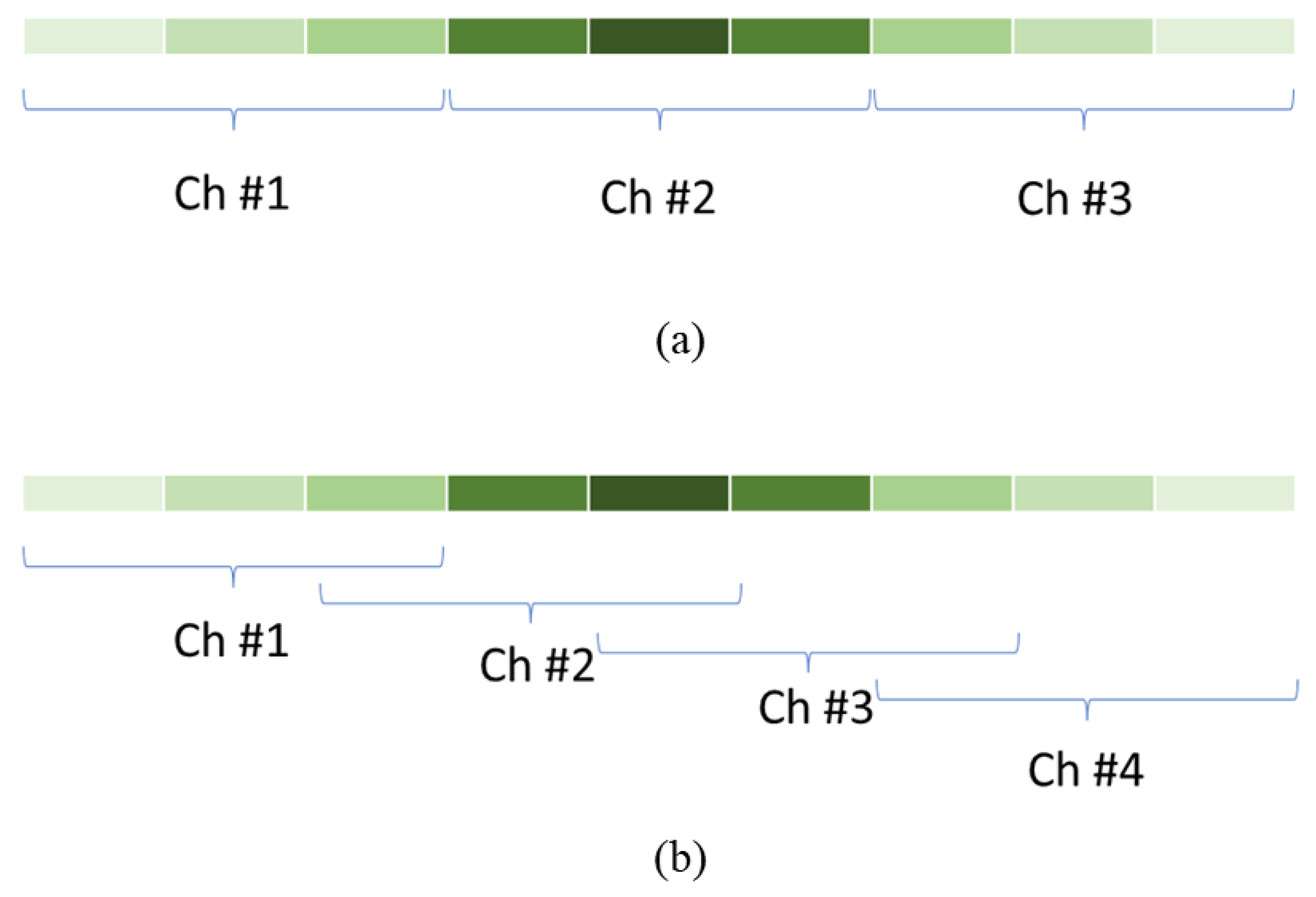
5.1. Generalized Uniform PRF

A MAPS system is designed to (i) maximize the swath coverage by keeping the PRF low and (ii) making the azimuth resolution finer by increasing the reconstructed azimuth bandwidth. At the same time, the level of ambiguity is kept low by on-ground digital beamforming. All these contrasting requirements imply the need for a high number of MAPS channels. According to the current theory, the maximum number of MAPS channels N is limited by the number of azimuth tiles of a phased-array SAR antenna, i.e., one tile corresponds to one receiving channel. Despite this, technological issues (e.g., limitations on the data volume) often limit the actual number of receiving channels to be lower than the maximum, forcing us to group more tiles into a single receiving channel.

Let us consider an exemplary case where a phased-array antenna owns nine azimuth tiles, but due to hardware limitations, the number of digital channels cannot be equal to nine. Using a classical design, the forced choice would be $N=3$ only, as in Figure 10a. However, we can overcome this limitation by allowing overlap between the channels. Due to the noise correlation in channels sharing the same receiving tiles, the recombination gain decreases (this is shown below), but the higher number of channels allows a lower PRF to be adopted, with a consequent advantage in swath coverage. The solution proposed in Figure 10b has $N=4$ partially overlapped digital channels. We show that this second system has more flexibility since it trades the final RG with more azimuth bandwidth, hence a better ambiguity rejection.

The uniform (or ideal) PRF ($PR{F}_{Uni}$), whose definition is in Equation (1), is the azimuth sampling frequency that fulfills the timing requirement for uniformly distributed samples. Sampling with the uniform $PR{F}_{Uni}$ or its multiples (not all the multiples are allowed; for details see [1,5,8]) provides a data array equivalent to that of a single-aperture (monostatic) system operating at $N·PRF$ frequency. Thus, the uniform $PR{F}_{Uni}$ allows a perfect spectrum reconstruction with the theoretical perfect rejection of the ambiguities up to the $N·PR{F}_{Uni}$ non-ambiguous frequency interval.

In the case of non-overlapping channels, the quantity $N·\Delta x_j$ in Equation (1) is always equal to the antenna length $L_a$. But in the case of overlapping channels, this statement no longer holds, and we also need to define the distance between MAPS channels $\Delta x_j$ as a multiple of the physical distance between two antenna tiles, $dx$.

Still referring to the two examples of Figure 10a and Figure 10b, we have $\Delta x_j=3dx$ in the first case and $\Delta x_j=2dx$ in the second case. This means that the uniform PRF of each case is:

$$\begin{array}{cc}\hfill PR{F}_{Uni,1}& ={\displaystyle \frac{2·v_s}{3·3dx}}={\displaystyle \frac{2·v_s}{L_a}}\hfill \\ \hfill PR{F}_{Uni,2}& ={\displaystyle \frac{2·v_s}{3·2dx}}={\displaystyle \frac{9}{8}}{\displaystyle \frac{2·v_s}{L_a}}\hfill \end{array}$$

(39)

The corresponding reconstructed spectrum is summarized in

Table 2. Relation between the number of MAPS channels and reconstructed non-ambiguous interval.

Case	# Az. Channels	Uniform PRF	Reconstructed Spectrum
non-Ov-MAPS	3	$2v_s/L_a$	$3·(2v_s/L_a)$
Ov-MAPS	4	$9/8·(2v_s/L_a)$	$9/2·(2v_s/L_a)$

for the two cases. As can be seen, the Ov-MAPS gains a 1.5 factor in the reconstructed spectrum with respect to the non-Ov-MAPS. This means that a higher azimuth resolution can be achieved starting from the two systems both acquiring at their uniform PRF (the achievable azimuth bandwidth is also a function of the main lobe azimuth pattern, which must be carefully designed). Moreover, the second system achieves a better ambiguity rejection, although the uniform PRF is quite close to the first system. However, the wider reconstructed spectrum is at the expense of the reduction in RG as shown in the next section.

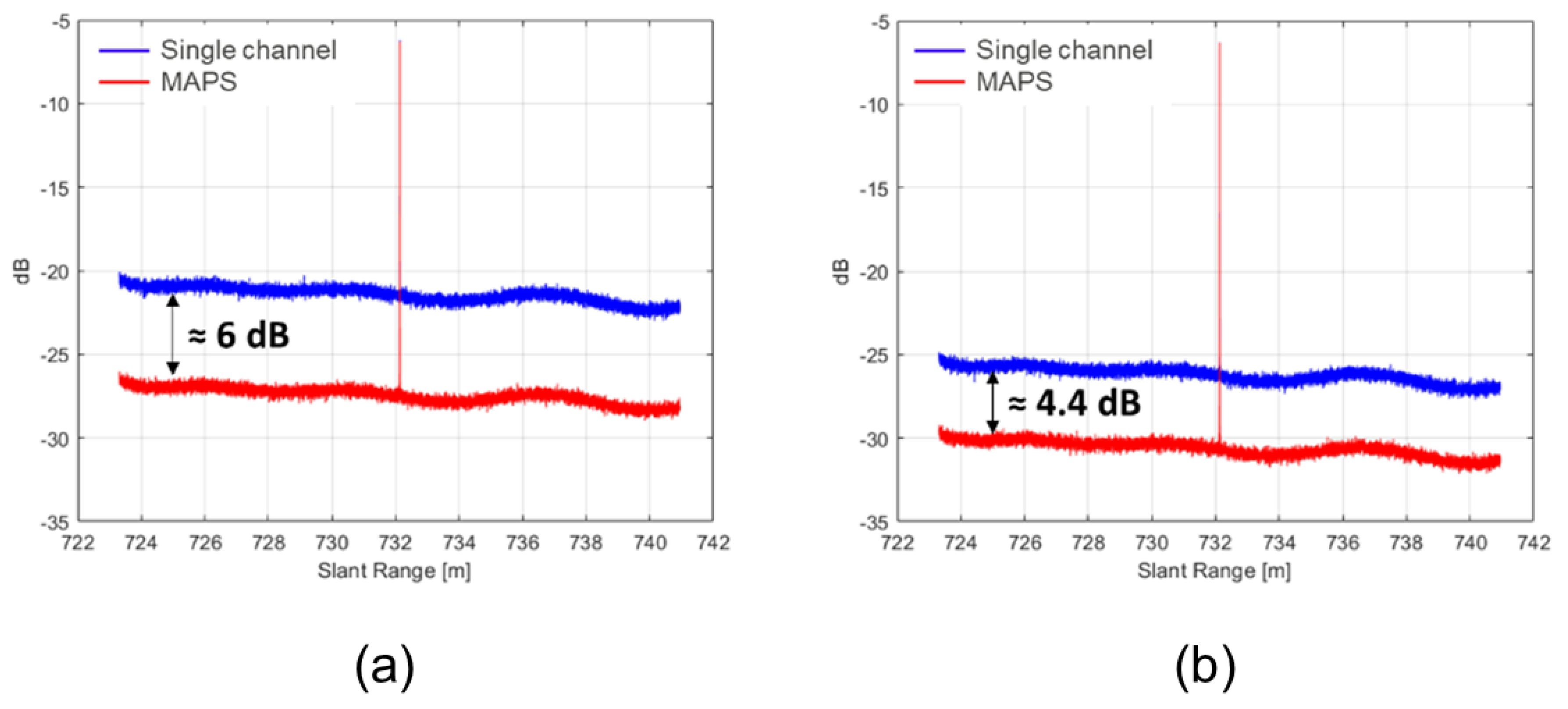
5.2. Recombination Gain for Overlapped MAPS

The price to be paid by the Ov-MAPS solution is a reduction in the RG and a worsening of the NESZ (or equivalently, the SNR) of the system. In a non-overlapped MAPS, the gain is $N^2$ times the power in each channel ($P_{s,1}$) since in ideal conditions, the signal sums coherently:

$$P_s=N^2·P_{s,1}$$

(40)

On the other hand, the gain of the noise is only N times the noise power in each channel since the noise sums incoherently:

$$P_s=N·P_{s,1}$$

(41)

The RG (with respect to the single RX channel) is defined according to [5]:

$$RG=\left({\displaystyle \frac{P_s}{P_n}}\right)/\left({\displaystyle \frac{P_{s,1}}{P_{n,1}}}\right)=N$$

(42)

To generalize the RG equation to the overlapping MAPS, we first define a channel matrix $\underline{\underline{M}}$, with N rows and $N_t$ columns, with $N_t$ the number of azimuth tiles. This matrix has one in position $(i,j)$ when the $j^{th}$ tile contributes to the $i^{th}$ digital channel. Then,

• The received power is still evaluated as a coherent sum, but it is achieved by summing all the terms coming from the receiving tiles in matrix $\underline{\underline{M}}$ multiplied by the number of digital channels N:

  $$P_s=\left(N·\sum _{i,j}\underline{\underline{M}}\right)·P_{s,1}$$

  (43)
• The noise is now partially correlated among the digital channels, so its covariance matrix is no longer diagonal, but we can still compute the total power by summing all the elements of the covariance matrix of the noise (${\underline{\underline{C}}}_n$):

  $$P_n=\sum _{i,j}{\underline{\underline{C}}}_n$$

  (44)

Eventually, plugging Equations (43) and (44) into Equation (42), the general expression of the RG is as follows:

$$RG={\displaystyle \frac{N·{\sum }_{i,j}\underline{\underline{M}}}{{\sum }_{i,j}{\underline{\underline{C}}}_n}}$$

(45)

The result in Equation (45) is the generalization to any MAPS configuration of the recombination gain (RG) defined for the first time in [5]. Note that this extension is not straightforward and represents a significant innovation to predict the performance (namely, the NESZ and SNR) of the MAPS with an architecture not limited to the non-Ov-MAPS. Moreover, to further state the generality of Equation (45), we highlight that the RG of the non-Ov-MAPS [5] is a particular case of Equation (45), where the numerator is $N^2$ and the denominator is N.

Before simulations (presented in Section 6), hereinafter, a couple of cases are proposed where the results from the previous section were applied to exemplary situations. In the following, the channel matrix was built for the two cases shown in Figure 10. Equation (46) is the channel matrix for the non-overlapped case, while Equation (47) refers to the overlapped case.

$${\underline{\underline{M}}}_1={\sigma }_s^2·\left[\begin{array}{ccccccccc}1& 1& 1& 0& 0& 0& 0& 0& 0\\ 0& 0& 0& 1& 1& 1& 0& 0& 0\\ 0& 0& 0& 0& 0& 0& 1& 1& 1\end{array}\right]$$

(46)

$${\underline{\underline{M}}}_2={\sigma }_s^2·\left[\begin{array}{ccccccccc}1& 1& 1& 0& 0& 0& 0& 0& 0\\ 0& 0& 1& 1& 1& 0& 0& 0& 0\\ 0& 0& 0& 0& 1& 1& 1& 0& 0\\ 0& 0& 0& 0& 0& 0& 1& 1& 1\end{array}\right]$$

(47)

Again, dealing with the noise covariance matrices, Equation (48) refers to the non-overlapped case while Equation (49) is for the overlapped MAPS:

$${\underline{\underline{C}}}_{n,1}={\sigma }_n^2·\left[\begin{array}{ccc}3& 0& 0\\ 0& 3& 0\\ 0& 0& 3\end{array}\right]$$

(48)

$${\underline{\underline{C}}}_{n,2}={\sigma }_n^2·\left[\begin{array}{cccc}3& 1& 0& 0\\ 1& 3& 1& 0\\ 0& 1& 3& 1\\ 0& 0& 1& 3\end{array}\right]$$

(49)

Then, according to Equation (46), with Equation (48), and to Equation (47), with Equation (49), we can evaluate the RG for the non-overlapped (see Equation (50)) and overlapped cases (see Equation (51)) by using Equation (45):

$$R{G}_1={\displaystyle \frac{N·{\sum }_{i,j}{\underline{\underline{M}}}_1}{{\sum }_{i,j}{\underline{\underline{C}}}_{n,1}}}={\displaystyle \frac{3·9}{9}}=3$$

(50)

$$R{G}_2={\displaystyle \frac{N·{\sum }_{i,j}{\underline{\underline{M}}}_2}{{\sum }_{i,j}{\underline{\underline{C}}}_{n,2}}}={\displaystyle \frac{4·12}{18}}=8/3$$

(51)

The overlapped MAPS loses $10{\log }_{10}(3/(8/3))\approx 0.51$ dB in RG with respect to the Ov-MAPS case, which results in an equal worsening of the NESZ of the latter with respect to the NESZ of the former. On the contrary, according to Equation (39) and Table 2, the Ov-MAPS provides a wider interval of Doppler frequency for the reconstructed spectrum which is expected to result in a better ambiguity-to-signal ratio.

5.3. Recombination Gain for Asymmetric MAPS

In the current section, we apply the theory of the channel matrix to an asymmetric MAPS. Let us assume a system with a phased-array antenna with seven azimuth tiles. According to Section 5.2, a way to introduce the MAPS technology into this system would be to consider three partially overlapped digital channels that would allow to (i) reduce the PRF by one-third and (ii) increase the swath width. The matrix channel of the Ov-MAPS configuration is:

$${\underline{\underline{M}}}_3={\sigma }_s^2·\left[\begin{array}{ccccccc}1& 1& 1& 0& 0& 0& 0\\ 0& 0& 1& 1& 1& 0& 0\\ 0& 0& 0& 0& 1& 1& 1\end{array}\right]$$

(52)

In this case, the noise covariance matrix is:

$${\underline{\underline{C}}}_{n,3}={\sigma }_n^2·\left[\begin{array}{ccc}3& 1& 0\\ 1& 3& 1\\ 0& 1& 3\end{array}\right]$$

(53)

However, the seven tiles of the phased-array antenna can also be arranged into an asymmetric, non-overlapped solution (As-MAPS), where the antenna columns 1–2 belong to the first digital channel, the columns 3–5 to the second one, and columns 6–7 to the last channel, thus avoiding overlapping. The channel matrix and noise covariance matrices are, respectively:

$${\underline{\underline{M}}}_4={\sigma }_s^2·\left[\begin{array}{ccccccc}1& 1& 0& 0& 0& 0& 0\\ 0& 0& 1& 1& 1& 0& 0\\ 0& 0& 0& 0& 0& 1& 1\end{array}\right]$$

(54)

$${\underline{\underline{C}}}_{n,4}={\sigma }_n^2·\left[\begin{array}{ccc}2& 0& 0\\ 0& 3& 0\\ 0& 0& 2\end{array}\right]$$

(55)

Please note that for the As-MAPS, the noise covariance matrix in Equation (55) is still diagonal, as for the no-Ov-MAPS, but now the elements have different values because of the different number of tiles for each MAPS channel.

Eventually, the recombination gain for the two configurations (i.e., Ov-MAPS and As-MAPS) is:

$$R{G}_3={\displaystyle \frac{3·9}{13}}=27/13$$

(56)

$$R{G}_4={\displaystyle \frac{3·7}{7}}=3$$

(57)

with an advantage of the second solution (i.e., As-MAPS) with respect to the first one of $10{\log }_{10}(3/(27/13))\approx 1.6$ dB in RG.

We remark here that using the As-MAPS instead of the Ov-MAPS when few digital channels are available may be a valuable solution to keep the denominator of the RG low when it is not possible to increase the number of digital channels N (e.g., for technological reasons). In particular, the As-MAPS avoids extra-diagonal elements of the noise covariance matrix limiting the sum of all the elements.

6. Simulation Results for Ov-MAPS and As-MAPS

This section presents two practical study cases: Section 6.1 is for the overlapping MAPS Section 6.2 is for the asymmetric MAPS. As for the bistatic MAPS in Section 4, simulations were carried out using a 1D end-to-end simulator with simplified geometry: a flat Earth and straight satellite trajectory were assumed. Despite these simplifications, the simulated data were fully suitable to prove the reliability of the theoretical models that we derived in the previous sections. The simulated 1D data inherently contained (i) the main signal plus azimuth ambiguities and (ii) the thermal noise. The MAPS reconstruction was performed using the MMSE algorithm. The point or distributed target scenes were used to evaluate the point and distributed target ambiguity ratio: AzPTAR and AzDTAR. Results of the non-overlapped and overlapped MAPS (Section 6.1) were compared, and the theoretical equations presented in Section 5 were validated.

6.1. Overlapped MAPS

In this case, a Sentinel-1-like antenna was designed but owning nine tiles. For this system, the solution with $N=3$ (no tiles’ overlap among the channels) and $N=4$ (tiles’ overlap), as in Figure 10, were compared. Both a point target and a distributed target were simulated, and the noise level was kept 30 dB below the point target energy (this choice was made to measure both the IRF parameters and the RG). During azimuth focusing, antenna whitening and a Hamming window of $0.85$ were applied.

Table 3. Sentinel-1-like parameters for the case study and performance estimation.

Parameter	Non-Ov-MAPS	Ov-MAPS	UoM
Carrier frequency	5.405		GHz
Antenna size	12.3		m
Uniform PRF	1237.4	1392.0	Hz
Actual PRF	2474.8	1392.0	Hz
PRF after reconstr.	7424.4	5568.0	Hz
# tiles	9		-
# digital channels	3	4	-
RG	4.77	4.26	dB
AzPTAR	−41.43	−51.19	dB
AzDTAR	−30.74	−34.99	dB
Azimuth res.	1.47	1.28	m

summarizes the main system parameters and performance.

Since the uniform PRF was different in the two configurations, a choice was made for the actual PRF, to obtain two systems comparable for the ambiguity rejection. For the non-Ov-MAPS, in the case of acquisition at the ideal PRF, the ambiguity suppression was very weak since the AzPTAR amounted to −21.44 dB while the AzDTAR amounted to −14.18 dB. For this reason, the PRF of the first system was doubled with respect to the ideal value.

From the reconstruction point of view, what is important is the capability to reject the first ambiguity, although in Table 3, the first not-solved ambiguity value is reported. Both systems completely removed the first ambiguity, as can be seen in Figure 11a,c (the blue line is the one-channel focused IRF, the red line is the reconstructed IRF). However, the Ov-MAPS, thanks to the four channels, also partially removed the second ambiguity (the one around ≈8 km, see Figure 11c); this explains the better result of the AzPTAR and AzDTAR in Table 3.

The level of the first not-solved ambiguity was very low in both cases but the Ov-MAPS allowed a larger swath coverage thanks to the reduced PRF adopted. The little price to be paid by the Ov-MAPS system was a loss of only 0.5 dB on the RG and on the NESZ (or equivalently, the SNR).

To verify the effective loss in the recombination gain when tiles were shared among adjacent channels, an end-to-end simulation was set up with a distributed target scene. In Figure 12, the gain in the NESZ is shown, when the NESZ of the single channel case is compared with the reconstructed one (from the full antenna). Two systems having both four digital channels were compared in the end-to-end simulation. In Figure 12a, the MAPS reconstruction for the four non-overlapped channels is considered. In this case, the gain was $10{\log }_{10}4\approx 6$ dB, as expected. In Figure 12b, the MAPS reconstruction for the four overlapped channels is considered. In this case, the gain with respect to the monostatic case should be $10{\log }_{10}2.667\approx 4.26$ dB (from Equation (51)), while 4.4 dB was estimated, which was comparable with the theoretical value.

6.2. Asymmetric MAPS

The case described in Section 5.3 was simulated. In this second example, the comparison was conducted between two systems having three digital channels, one with overlapping, the other using non-overlapped but asymmetrical channels.

Table 4. System parameters for the case study and performance estimation.

Parameter	Ov-MAPS	As-MAPS	UoM
Carrier frequency	5.405		GHz
Antenna size	9.55		m
Uniform PRF	1856.1	1484.9	Hz
Actual PRF	1856.1	1484.9	Hz
PRF after reconstr.	5568.3	4454.7	Hz
# tiles	7		-
# digital channels	3		-
RG	3.17	4.77	dB
AzPTAR	−67.18	−31.99	dB
AzDTAR	−40.28	−27.04	dB
Azimuth res.	4.52	4.58	m

summarizes the main system parameters and performance results.

Again, we underline the capability of the system to completely remove the first ambiguity, as shown in Figure 13. The first not-solved ambiguity was still good for the asymmetric MAPS case, being about $-32$ dB for the point target and $-27$ dB for the distributed target. The advantage of the asymmetric solution in this case was (i) the lower PRF, from which a higher swath coverage can be achieved and (ii) a higher recombination gain (see Equations (56) and (57)), thus a noise sensitivity (measured by the NESZ) $1.6$ dB better.

7. Discussion and Conclusions

In this theoretical paper, we proposed a first approach to the generalization of the SAR azimuth multichannel system (MAPS) towards non-conventional configurations, both in terms of sensors’ deployment and/or multiple azimuth channels’ organization.

Dealing with the first topic, we considered formations with a bistatic baseline well beyond the canonical quasi-monostatic approximation, and we proposed two methods to solve the MAPS recombination in this configuration. In Section 3.2, we extended the approach of considering MAPS as the inversion of a Linear, Time-Invariant (LTI) filter. Indeed, this represents a mathematical interpretation of the problem and it is relevant since it uses the same approach widely assumed in the scientific literature for single platform–zero Doppler (SP-ZD) systems. Instead, in Section 3.3, we tackled the problem of MAPS reconstruction from a physical point of view by resorting to the key equivalence of SAR, i.e., Doppler frequencies are azimuth angles of arrival of the signal. According to the theory of DoA, we implemented a MAPS reconstruction based on Minimum Variance Distortionless Reconstruction (MVDR, or Capon beamformer). Specific corrections for a bistatic acquisition were analyzed and implemented. For both approaches (i.e., LTI and DoA), we performed a sensitivity analysis considering a likely SAR sensor operated in the L-band and C-band. The experimental results pointed out the limits of the LTI implementation when the SAR system worked in a condition far from the bistatic zero Doppler. The worsening of the LTI-MAPS performance was more pronounced for the C-band (with respect to the L-band) because of its shorter wavelength. These results were expected and in full agreement with the literature [11,12], but it was still meaningful to show that if the LTI method is selected, a semi-numerical approach is mandatory. Conversely, the results of the DoA-MAPS turned out to be effective in reducing the level of the first ambiguity also for Doppler centroids far from zero. Further analyses are underway to clarify some details of the experimental results and to verify the effectiveness of the method also in case of a realistic geometry with curved trajectory and an ellipsoidal Earth.

The second part of the paper was about how to organize the tiles of the SAR antenna into azimuth channels. Differently from the literature, in this paper, partially overlapped or asymmetric channels were considered, to let the system have more degree of freedom to spend between a larger swath coverage (which is a function of the actual PRF) and a better noise sensitivity through the RG, which straightly impacts on the pattern directivity. To prove the theoretical equations that predict the RG for both Ov-MAPS and As-MAPS, two cases were considered. In the first case, we made a comparison between Ov-MAPS and non-Ov-MAPS. We showed an example where, by sacrificing a little in the noise sensitivity ($0.5$ dB), a wider swath coverage could be obtained thanks to a lower PRF with respect to the one of the same instrument operated in the no-Ov-MAPS (i.e., only 56% of the not-overlapped MAPS). In a second case, a further improvement over the Ov-MAPS was achieved by using an As-MAPS. The advantages of the latter are in both PRF reduction (equal to only 80% of that of the Ov-MAPS) and recombination gain ($1.6$ dB gained with respect to Ov-MAPS).

In future work, a more detailed analysis will be performed by including the SAR timing diagram and evaluating this way the effective swath coverage when PRF changes. Moreover, actual mission parameters will be included to show the capability of generalizing the MAPS technology for current or future missions.

References

1. Gebert, N.; Krieger, G.; Moreira, A. Digital Beamforming on Receive: Techniques and Optimization Strategies for High-Resolution Wide-Swath SAR Imaging. IEEE Trans. Aerosp. Electron. Syst. 2009, 45, 564–592. [Google Scholar] [CrossRef]
2. Geudtner, D.; Tossaint, M.; Davidson, M.; Torres, R. Copernicus Sentinel-1 Next Generation Mission. In Proceedings of the 2021 IEEE International Geoscience and Remote Sensing Symposium IGARSS, Brussels, Belgium, 11–16 July 2021; pp. 874–876. [Google Scholar] [CrossRef]
3. Davidson, M.; Kubanek, J.; Iannini, L.; Furnell, R.; Di Cosimo, G.; Gebert, N.; Petrolati, D.; Geudtner, D.; Osborne, S. Rose-L—The Copernicus L-Band Synthetic Aperture Radar Imaging Mission. In Proceedings of the IGARSS 2023—2023 IEEE International Geoscience and Remote Sensing Symposium, Pasadena, CA, USA, 16–21 July 2023; pp. 4568–4571. [Google Scholar] [CrossRef]
4. Krieger, G.; Gebert, N.; Moreira, A. Unambiguous SAR signal reconstruction from nonuniform displaced phase center sampling. IEEE Geosci. Remote Sens. Lett. 2004, 1, 260–264. [Google Scholar] [CrossRef]
5. Giudici, D.; Guccione, P.; Manzoni, M.; Guarnieri, A.M.; Rocca, F. Compact and Free-Floating Satellite MIMO SAR Formations. IEEE Trans. Geosci. Remote Sens. 2022, 60, 1000212. [Google Scholar] [CrossRef]
6. Guccione, P.; Monti Guarnieri, A.; Rocca, F.; Giudici, D.; Gebert, N. Along-Track Multistatic Synthetic Aperture Radar Formations of Minisatellites. Remote Sens. 2020, 12, 124. [Google Scholar] [CrossRef]
7. Aguttes, J. The SAR train concept: Required antenna area distributed over N smaller satellites, increase of performance by N. In Proceedings of the IGARSS 2003. 2003 IEEE International Geoscience and Remote Sensing Symposium, Toulouse, France, 21–25 July 2023; Proceedings (IEEE Cat. No.03CH37477). IEEE: New York, NY, USA, 2003; Volume 1, pp. 542–544. [Google Scholar] [CrossRef]
8. Gebert, N.; Krieger, G.; Moreira, A. Multichannel Azimuth Processing in ScanSAR and TOPS Mode Operation. IEEE Trans. Geosci. Remote Sens. 2010, 48, 2994–3008. [Google Scholar] [CrossRef]
9. Kraus, T.; Krieger, G.; Bachmann, M.; Moreira, A. Spaceborne Demonstration of Distributed SAR Imaging With TerraSAR-X and TanDEM-X. IEEE Geosci. Remote Sens. Lett. 2019, 16, 1731–1735. [Google Scholar] [CrossRef]
10. Gebert, N.; Krieger, G. Azimuth Phase Center Adaptation on Transmit for High-Resolution Wide-Swath SAR Imaging. IEEE Geosci. Remote Sens. Lett. 2009, 6, 782–786. [Google Scholar] [CrossRef]
11. Neo, Y.L.; Wong, F.; Cumming, I.G. A Two-Dimensional Spectrum for Bistatic SAR Processing Using Series Reversion. IEEE Geosci. Remote Sens. Lett. 2007, 4, 93–96. [Google Scholar] [CrossRef]
12. D’Aria, D.; Monti Guarnieri, A. High-Resolution Spaceborne SAR Focusing by SVD-Stolt. IEEE Geosci. Remote Sens. Lett. 2007, 4, 639–643. [Google Scholar] [CrossRef]
13. McDonough, R.N.; Curlander, J.C. Synthetic Aperture Radar: Systems and Signal Processing; John Wiley and Sons: Hoboken, NJ, USA, 1992; p. 672. [Google Scholar]
14. Eranti, P.K.; Barkana, B.D. An Overview of Direction-of-Arrival Estimation Methods Using Adaptive Directional Time-Frequency Distributions. Electronics 2022, 11, 1321. [Google Scholar] [CrossRef]
15. Jeong, S.H.; Son, B.k.; Lee, J.H. Asymptotic Performance Analysis of the MUSIC Algorithm for Direction-of-Arrival Estimation. Appl. Sci. 2020, 10, 63. [Google Scholar] [CrossRef]
16. Capon, J. High-resolution frequency-wavenumber spectrum analysis. Proc. IEEE 1969, 57, 1408–1418. [Google Scholar] [CrossRef]
17. Guo, X.; Wan, Q.; Zhang, Y.; Liang, J. Teaching notes of MVDR in digital signal processing (DSP). In Proceedings of the IEEE International Conference on Teaching, Assessment, and Learning for Engineering (TALE) 2012, Hong Kong, China, 20–23 August 2012; pp. H3A-5–H3A-8. [Google Scholar] [CrossRef]
18. Mora, O.; Agustí, O.; Bara, M.; Broquetas, A. Direct geocoding for generation of precise wide-area elevation models with ERS SAR data. In Proceedings of the Fringe’99: Advancing ERS, SAR Interferometry from Applications towards Operations, Liège, Belgium, 10–12 November 1999; ESA: Paris, France, 2000. [Google Scholar]
19. Small, D.; Schubert, A. Guide to Sentinel-1 Geocoding; Technical Report UZHS1-GC-AD; Remote Sensing Laboratory University of Zurich (RSL): Zurich, Swetzerland, 2022; p. 42. [Google Scholar]
20. Villano, M.; Krieger, G. Impact of Azimuth Ambiguities on Interferometric Performance. IEEE Geosci. Remote Sens. Lett. 2012, 9, 896–900. [Google Scholar] [CrossRef]
21. Zonno, M.; Richter, D.; Thaniyil Prabhakaran, A.; Rodriguez Cassola, M.; Zurita Campos, A.; Del Castillo Mena, J.; Olea Garcia, A. Impact of coherent ambiguities on InSAR performance for bistatic SAR missions: The Harmony mission case. In Proceedings of the EUSAR 2022, 14th European Conference on Synthetic Aperture Radar, Leipzig, Germany, 25–27 July 2022; pp. 1–6. [Google Scholar]
22. López-Dekker, P.; Li, Y.; Iannini, L.; Prats-Iraola, P.; Rodríguez-Cassola, M. On Azimuth Ambiguities Suppression for Short-Baseline Along-Track Interferometry: The Stereoid Case. In Proceedings of the IGARSS 2019—2019 IEEE International Geoscience and Remote Sensing Symposium, Yokohama, Japan, 28 July–2 August 2019; pp. 110–113. [Google Scholar] [CrossRef]
23. Yi, N.; He, Y.; Liu, B. Improved Method to Suppress Azimuth Ambiguity for Current Velocity Measurement in Coastal Waters Based on ATI-SAR Systems. Remote Sens. 2020, 12, 3288. [Google Scholar] [CrossRef]
24. Guarnieri, A. Adaptive removal of azimuth ambiguities in SAR images. IEEE Trans. Geosci. Remote Sens. 2005, 43, 625–633. [Google Scholar] [CrossRef]
25. Richter, D.; Rodriguez-Cassola, M.; Zonno, M.; Prats-Iraola, P. Coherent Azimuth Ambiguity Suppression Based on Linear Optimum Filtering of Short Along-Track Baseline SAR Interferograms. In Proceedings of the EUSAR 2022, 14th European Conference on Synthetic Aperture Radar, Leipzig, Germany, 25–27 July 2022; pp. 1–5. [Google Scholar]
Figure 1. Reference bistatic geometry for the MAPS. Tx is green, Rx’s are orange, and the generic scatterer is black. Three examples are considered: (a) α = 0.5 ; (b) α = 0.0 ; (c) α = 1.0 .
Remotesensing 16 03170 g001
Figure 2. Processing scheme for LTI-MAPS.
Remotesensing 16 03170 g002
Figure 3. Zero-Doppler acquisition: (a) bistatic geometry; (b) monostatic geometry.
Remotesensing 16 03170 g003
Figure 4. Processing scheme for MVDR-MAPS.
Remotesensing 16 03170 g004
Figure 5. Sensitivity analysis of the MAPS as an LTI filter. Left panel: L-band; right panel: C-band. The two images report the gain on the FAAzPTAR as a function of the Tx-Rx distance Δ x 0 (y-axis) and the corresponding normalized bistatic Doppler centroid α (x-axis). The same color scale is used to facilitate the comparison.
Remotesensing 16 03170 g005
Figure 6. MAPS as an LTI filter: IRF for α = 0.5 ; Δ x 0 = 400 km. Left panels: L-band; right panels: C-band. Top panels: focused IRF up to the first azimuth ambiguity. Bottom panels: Doppler spectra. Blue lines are for the single channel data, and orange lines are for MAPS data.
Remotesensing 16 03170 g006aRemotesensing 16 03170 g006b
Figure 7. MAPS as an LTI filter: IRF for α = 1 ; Δ x 0 = 400 km. L-band. Left panel: focused IRF up to the first azimuth ambiguity. Right panel: Doppler spectra. Blue lines are for the single channel data, and orange lines are for MAPS data.
Remotesensing 16 03170 g007
Figure 8. Sensitivity analysis of the MAPS as a DoA estimation. Left panel: L-band; right panel: C-band. The two images report the gain on the FAAzPTAR as a function of the Tx-Rx distance Δ x 0 (y-axis) and the corresponding normalized bistatic Doppler centroid α (x-axis). The same color scale is used to facilitate the comparison.
Remotesensing 16 03170 g008
Figure 9. MAPS as a DoA estimation: IRF for α = 1 ; Δ x 0 = 400 km. L-band. Left panel: focused IRF up to the first azimuth ambiguity. Right panel: Doppler spectra. Blue lines are for the single channel data, and orange lines are for MAPS data.
Remotesensing 16 03170 g009
Figure 10. Nine-tile phased-array antenna. (a) Three-non-overlapped-channel MAPS case; (b) Four-overlapped-channel MAPS cases. Tiles’ color is for aesthetic reasons only.
Remotesensing 16 03170 g010
Figure 11. Non-Ov-MAPS (top row) vs. Ov-MAPS (bottom row) simulation cases. (ac) IRF (single-channel and reconstructed); (bd) power spectral density.
Remotesensing 16 03170 g011
Figure 12. NESZ as a function of slant range. (a) Non-Ov-MAPS; (b) Ov-MAPS. Both systems have N = 4 digital channels.
Remotesensing 16 03170 g012
Figure 13. Ov-MAPS (top row) vs. Asym-MAPS (bottom row) simulation cases. (ac) IRF (single-channel and reconstructed); (bd) power spectral density.
Remotesensing 16 03170 g013