
At Which Overpass Time Do ECOSTRESS Observations Best Align with Crop Health and Water Rights?
 , ,
, ,
Abstract
:1. Introduction
- Examine how ESI observations vary based on their acquisition time;
- Evaluate how closely ESI aligns with crop health and water rights;
- Assess the potential for ESI to capture sub-optimal crop conditions.
2. Data and Methods
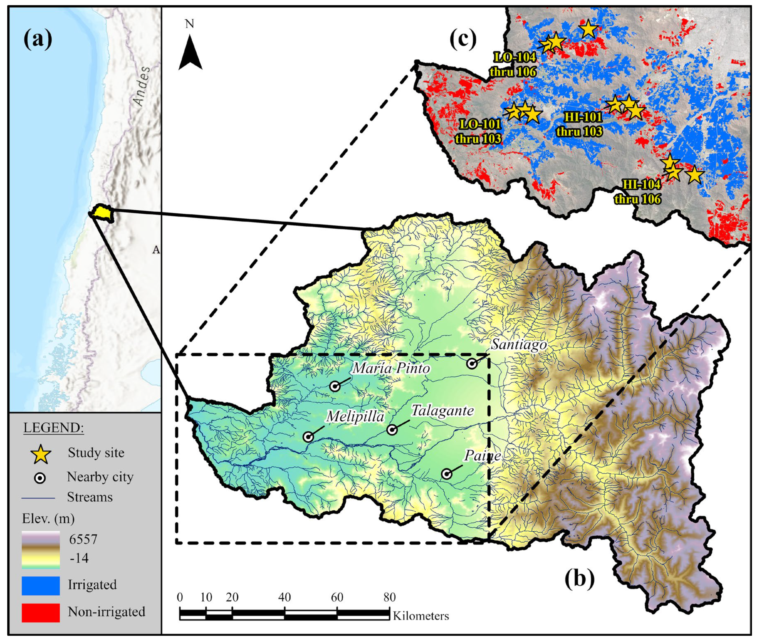
2.1. Study Area
2.2. Earth Observations
- the morning hours from 5:00 a.m. to 9:59 a.m.; and
- the afternoon hours from 12:00 p.m. to 4:59 p.m.
- 2019 to 2020;
- 2020 to 2021;
- 2021 to 2022.
2.3. Selection of Maize Site at the Parcel Level
2.4. Compilation of Water Allocations at the Regional Scale
3. Results
3.1. Temporal Patterns in ESI at Selected Maize Fields
3.2. Spatial Patterns in ESI throughout the Agricultural Land
3.3. Spatial Correlation of ESI with Crop Health
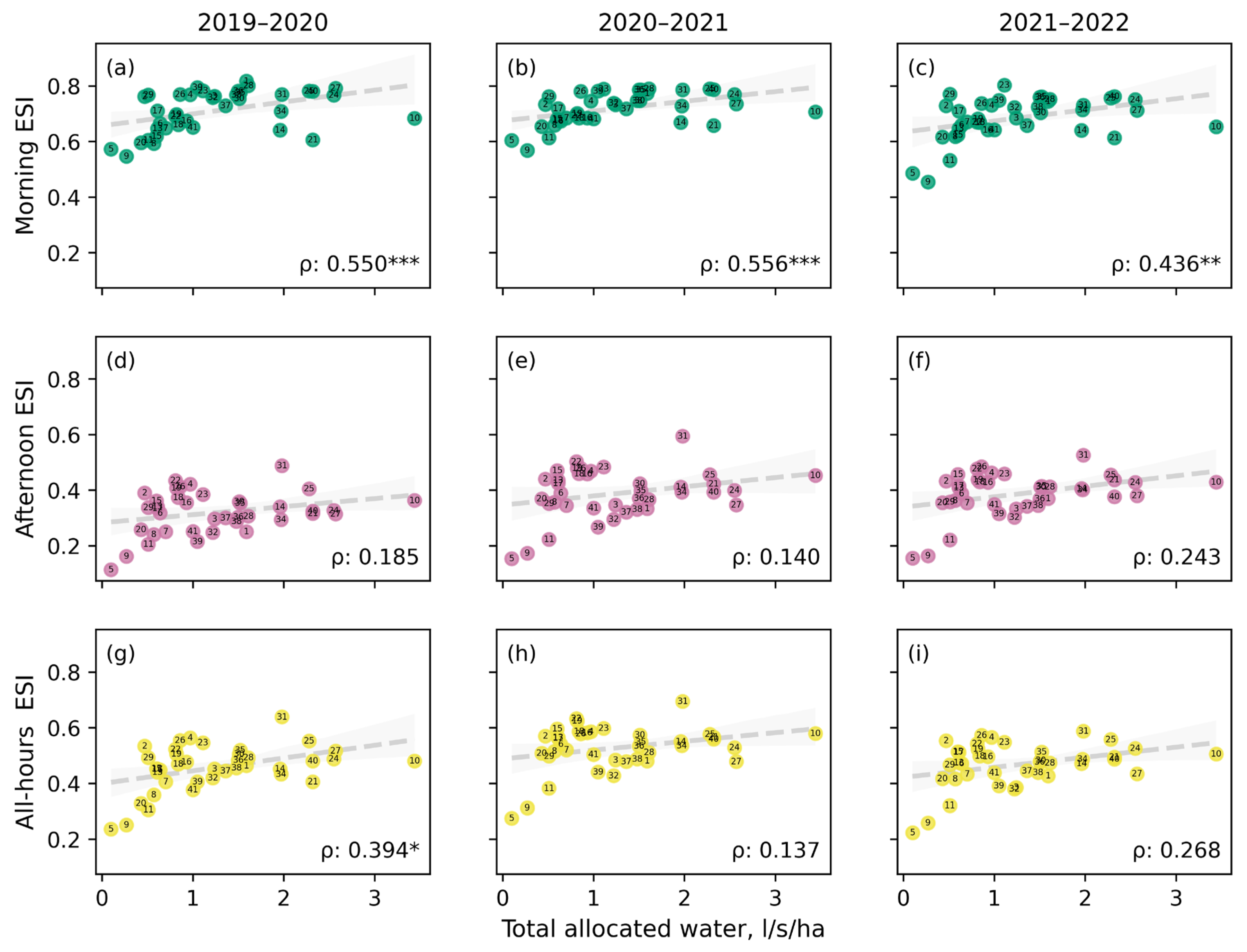
3.4. Correlation of ESI with Water Rights
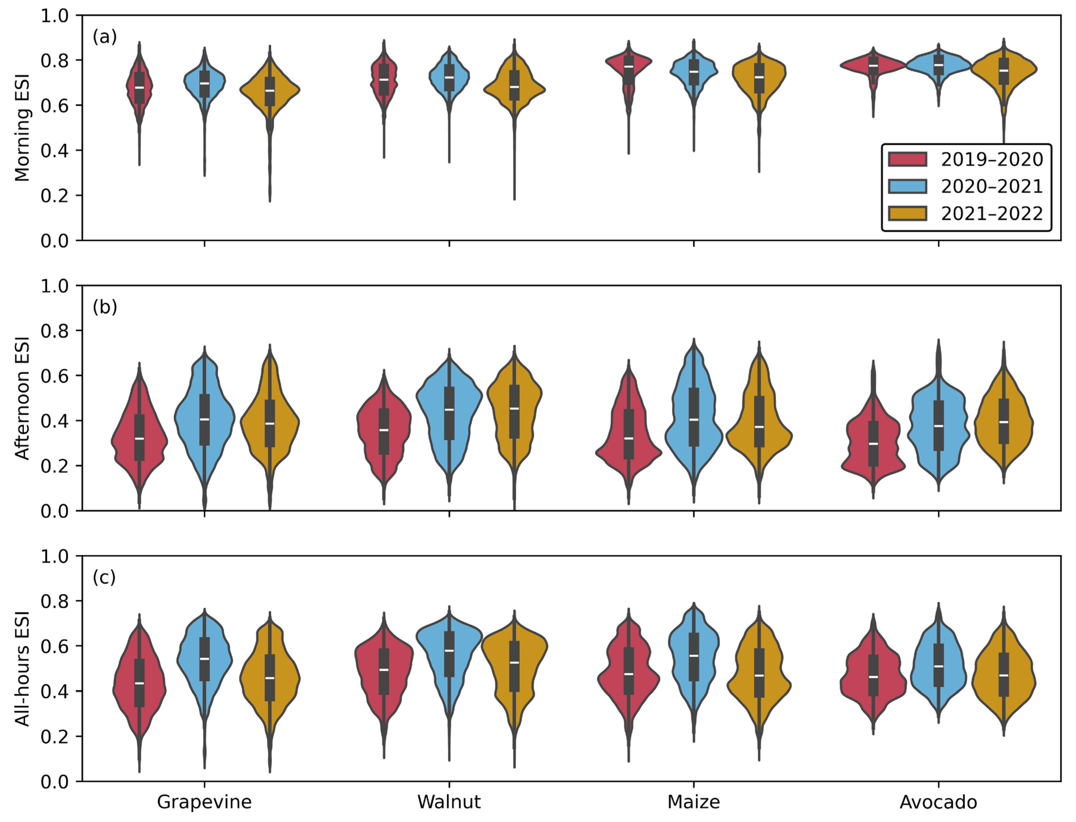
3.5. Variations in Crop Productions
4. Discussion
4.1. Need for ECOSTRESS ESI
4.2. Limited Understanding of ECOSTRESS ESI
4.3. New Insights into ECOSTRESS ESI
4.4. Societal Implications
4.5. Future Work
5. Conclusions
Supplementary Materials
Author Contributions
Funding
Data Availability Statement
Acknowledgments
Conflicts of Interest
References
- Sauer, T.; Havlík, P.; Schneider, U.A.; Schmid, E.; Kindermann, G.; Obersteiner, M. Agriculture and resource availability in a changing world: The role of irrigation. Water Resour. Res. 2010, 46, e2009WR007729. [Google Scholar] [CrossRef]
- Howden, S.M.; Soussana, J.F.; Tubiello, F.N.; Chhetri, N.; Dunlop, M.; Meinke, H. Adapting agriculture to climate change. Proc. Natl. Acad. Sci. USA 2007, 104, 19691–19696. [Google Scholar] [CrossRef] [PubMed]
- Heim, R.R., Jr. A review of twentieth-century drought indices used in the United States. Bull. Am. Meteorol. Soc. 2002, 83, 1149–1166. [Google Scholar] [CrossRef]
- Fisher, J.B.; Whittaker, R.J.; Malhi, Y. ET come home: Potential evapotranspiration in geographical ecology. Glob. Ecol. Biogeogr. 2011, 20, 1–18. [Google Scholar] [CrossRef]
- Begg, J.E.; Turner, N.C. Crop water deficits. Adv. Agron. 1976, 28, 161–217. [Google Scholar] [CrossRef]
- Wang, K.; Dickinson, R.E. A review of global terrestrial evapotranspiration: Observation, modeling, climatology, and climatic variability. Rev. Geophys. 2012, 50, e2011RG000373. [Google Scholar] [CrossRef]
- Lobell, D.B.; Gourdji, S.M. The influence of climate change on global crop productivity. Plant Physiol. 2012, 160, 1686–1697. [Google Scholar] [CrossRef]
- Narasimhan, B.; Srinivasan, R. Development and evaluation of Soil Moisture Deficit Index (SMDI) and Evapotranspiration Deficit Index (ETDI) for agricultural drought monitoring. Agric. For. Meteorol. 2005, 133, 69–88. [Google Scholar] [CrossRef]
- Koehler, T.; Wankmüller, F.J.; Sadok, W.; Carminati, A. Transpiration response to soil drying vs. increasing vapor pressure deficit in crops–physical and physiological mechanisms and key plant traits. J. Exp. Bot. 2023, 74, 4789–4807. [Google Scholar] [CrossRef]
- Nelson, G.C.; Rosegrant, M.W.; Koo, J.; Robertson, R.; Sulser, T.; Zhu, T.; Ringler, C.; Msangi, S.; Palazzo, A.; Batka, M.; et al. Climate Change: Impact on Agriculture and Costs of Adaptation; International Food Policy Research Institute (IFPRI): Washington, DC, USA, 2009; Volume 21, Available online: https://ebrary.ifpri.org/utils/getfile/collection/p15738coll2/id/130648/filename/130821.pdf (accessed on 23 July 2024).
- Dai, A. Drought under global warming: A review. Wiley Interdiscip. Rev. Clim. Chang. 2011, 2, 45–65. [Google Scholar] [CrossRef]
- Fisher, J.B.; Melton, F.; Middleton, E.; Hain, C.; Anderson, M.; Allen, R.; McCabe, M.F.; Hook, S.; Baldocchi, D.; Townsend, P.A.; et al. The future of evapotranspiration: Global requirements for ecosystem functioning, carbon and climate feedbacks, agricultural management, and water resources. Water Resour. Res. 2017, 53, 2618–2626. [Google Scholar] [CrossRef]
- Fisher, J.B. Level-4 Evaporative Stress Index L4 (ESI_PT-JPL) Algorithm Theoretical Basis Document; JPL: Pasadena, CA, USA, 2018. Available online: https://lpdaac.usgs.gov/documents/342/ECO4ESIPTJPL_ATBD_V1.pdf (accessed on 23 July 2024).
- Anderson, M.C.; Hain, C.; Wardlow, B.; Pimstein, A.; Mecikalski, J.R.; Kustas, W.P. Evaluation of drought indices based on thermal remote sensing of evapotranspiration over the continental United States. J. Clim. 2011, 24, 2025–2044. [Google Scholar] [CrossRef]
- Anderson, M.C.; Kustas, W.P.; Norman, J.M.; Hain, C.R.; Mecikalski, J.R.; Schultz, L.; González-Dugo, M.P.; Cammalleri, C.; D‘Urso, G.; Pimstein, A.; et al. Mapping daily evapotranspiration at field to continental scales using geostationary and polar orbiting satellite imagery. Hydrol. Earth Syst. Sci. 2011, 15, 223–239. [Google Scholar] [CrossRef]
- Anderson, M.C.; Hain, C.; Otkin, J.; Zhan, X.; Mo, K.; Svoboda, M.; Wardlow, B.; Pimstein, A. An intercomparison of drought indicators based on thermal remote sensing and NLDAS-2 simulations with US Drought Monitor classifications. J. Hydrometeorol. 2013, 14, 1035–1056. [Google Scholar] [CrossRef]
- Otkin, J.A.; Anderson, M.C.; Hain, C.; Mladenova, I.E.; Basara, J.B.; Svoboda, M. Examining rapid onset drought development using the thermal infrared–based evaporative stress index. J. Hydrometeorol. 2013, 14, 1057–1074. [Google Scholar] [CrossRef]
- Anderson, M.C.; Zolin, C.A.; Sentelhas, P.C.; Hain, C.R.; Semmens, K.; Yilmaz, M.T.; Gao, F.; Otkin, J.A.; Tetrault, R. The Evaporative Stress Index as an indicator of agricultural drought in Brazil: An assessment based on crop yield impacts. Remote Sens. Environ. 2016, 174, 82–99. [Google Scholar] [CrossRef]
- Otkin, J.A.; Anderson, M.C.; Hain, C.; Svoboda, M.; Johnson, D.; Mueller, R.; Tadesse, T.; Wardlow, B.; Brown, J. Assessing the evolution of soil moisture and vegetation conditions during the 2012 United States flash drought. Agric. For. Meteorol. 2016, 218, 230–242. [Google Scholar] [CrossRef]
- Nguyen, H.; Wheeler, M.C.; Otkin, J.A.; Cowan, T.; Frost, A.; Stone, R. Using the evaporative stress index to monitor flash drought in Australia. Environ. Res. Lett. 2019, 14, 064016. [Google Scholar] [CrossRef]
- Anderson, M.C.; Norman, J.M.; Mecikalski, J.R.; Otkin, J.A.; Kustas, W.P. A climatological study of evapotranspiration and moisture stress across the continental United States based on thermal remote sensing: 2. Surface moisture climatology. J. Geophys. Res. Atmos. 2007, 112, e2006JD007507. [Google Scholar] [CrossRef]
- Fisher, J.B.; Lee, B.; Purdy, A.J.; Halverson, G.H.; Dohlen, M.B.; Cawse-Nicholson, K.; Wang, A.; Anderson, R.G.; Aragon, B.; Arain, M.A.; et al. ECOSTRESS: NASA’s next generation mission to measure evapotranspiration from the international space station. Water Resour. Res. 2020, 56, e2019WR026058. [Google Scholar] [CrossRef]
- Hulley, G.; Hook, S.; Fisher, J.; Lee, C. ECOSTRESS, A NASA Earth-Ventures Instrument for studying links between the water cycle and plant health over the diurnal cycle. In Proceedings of the 2017 IEEE International Geoscience and Remote Sensing Symposium (IGARSS), Fort Worth, TX, USA, 23–28 July 2017; pp. 5494–5496. [Google Scholar] [CrossRef]
- Fisher, J.B.; Tu, K.P.; Baldocchi, D.D. Global estimates of the land–atmosphere water flux based on monthly AVHRR and ISLSCP-II data, validated at 16 FLUXNET sites. Remote Sens. Environ. 2008, 112, 901–919. [Google Scholar] [CrossRef]
- Fisher, J.B. Level-3 Evapotranspiration L3 (ET_PT-JPL) Algorithm Theoretical Basis Document; JPL: Pasadena, CA, CA, USA, 2018. Available online: https://lpdaac.usgs.gov/documents/335/ECO3ETPTJPL_ATBD_V1.pdf (accessed on 23 July 2024).
- Xiao, J.; Fisher, J.B.; Hashimoto, H.; Ichii, K.; Parazoo, N.C. Emerging satellite observations for diurnal cycling of ecosystem processes. Nat. Plants 2021, 7, 877–887. [Google Scholar] [CrossRef] [PubMed]
- Chen, Y.; Xia, J.; Liang, S.; Feng, J.; Fisher, J.B.; Li, X.; Li, X.; Liu, S.; Ma, Z.; Miyata, A.; et al. Comparison of satellite-based evapotranspiration models over terrestrial ecosystems in China. Remote Sens. Environ. 2014, 140, 279–293. [Google Scholar] [CrossRef]
- Ershadi, A.; McCabe, M.F.; Evans, J.P.; Chaney, N.W.; Wood, E.F. Multi-site evaluation of terrestrial evaporation models using FLUXNET data. Agric. For. Meteorol. 2014, 187, 46–61. [Google Scholar] [CrossRef]
- McCabe, M.F.; Ershadi, A.; Jimenez, C.; Miralles, D.G.; Michel, D.; Wood, E.F. The GEWEX LandFlux project: Evaluation of model evaporation using tower-based and globally gridded forcing data. Geosci. Model Dev. 2016, 9, 283–305. [Google Scholar] [CrossRef]
- Michel, D.; Jiménez, C.; Miralles, D.G.; Jung, M.; Hirschi, M.; Ershadi, A.; Martens, B.; McCabe, M.F.; Fisher, J.B.; Mu, Q.; et al. The WACMOS-ET project–Part 1: Tower-scale evaluation of four remote-sensing-based evapotranspiration algorithms. Hydrol. Earth Syst. Sci. 2016, 20, 803–822. [Google Scholar] [CrossRef]
- Liu, N.; Oishi, A.C.; Miniat, C.F.; Bolstad, P. An evaluation of ECOSTRESS products of a temperate montane humid forest in a complex terrain environment. Remote Sens. Environ. 2021, 265, 112662. [Google Scholar] [CrossRef]
- Wu, J.; Feng, Y.; Liang, L.; He, X.; Zeng, Z. Assessing evapotranspiration observed from ECOSTRESS using flux measurements in agroecosystems. Agric. Water Manag. 2022, 269, 107706. [Google Scholar] [CrossRef]
- Liang, L.; Feng, Y.; Wu, J.; He, X.; Liang, S.; Jiang, X.; de Oliveira, G.; Qiu, J.; Zeng, Z. Evaluation of ECOSTRESS evapotranspiration estimates over heterogeneous landscapes in the continental US. J. Hydrol. 2022, 613, 128470. [Google Scholar] [CrossRef]
- Hu, T.; Mallick, K.; Hitzelberger, P.; Didry, Y.; Boulet, G.; Szantoi, Z.; Koetz, B.; Alonso, I.; Pascolini-Campbell, M.; Halverson, G.; et al. Evaluating European ECOSTRESS Hub Evapotranspiration Products Across a Range of Soil-Atmospheric Aridity and Biomes Over Europe. Water Resour. Res. 2023, 59, e2022WR034132. [Google Scholar] [CrossRef]
- Pascolini-Campbell, M.; Lee, C.; Stavros, N.; Fisher, J.B. ECOSTRESS reveals pre-fire vegetation controls on burn severity for Southern California wildfires of 2020. Glob. Ecol. Biogeogr. 2022, 31, 1976–1989. [Google Scholar] [CrossRef]
- Goffin, B.D.; Thakur, R.; Carlos, S.D.C.; Srsic, D. Maipo River Valley Agriculture: Determining Crop Coefficients Using Remote Sensing for the Maipo River Valley Basin in Chile. NASA DEVELOP National Program: Virginia—LaRC, 2022. [Unpublished Manuscript]. Available online: https://ntrs.nasa.gov/api/citations/20220013971/downloads/2022Sum_PUP_MaipoRiverValleyAg_TechPaper_FD_v2.docx.pdf (accessed on 23 July 2024).
- Fritz, S.; See, L.; Bayas, J.C.L.; Waldner, F.; Jacques, D.; Becker-Reshef, I.; Whitcraft, A.; Baruth, B.; Bonifacio, R.; Crutchfield, J.; et al. A comparison of global agricultural monitoring systems and current gaps. Agric. Syst. 2019, 168, 258–272. [Google Scholar] [CrossRef]
- Dirección General de Aguas (DGA); Centro de Información de Recursos Naturales (CIREN). Redefinición de la Clasificación Red Hidrográfica a Nivel Nacional; Dirección General de Aguas (DGA): Santiago, Chile, 2014; Available online: https://snia.mop.gob.cl/repositoriodga/handle/20.500.13000/6786 (accessed on 1 December 2023).
- Centro de Información de Recursos Naturales (CIREN). Progama de Actualización de Cobertura y Uso de Suelo Agrícola: Región de Valparaíso; CIREN: Santiago, Chile, 2020. [Google Scholar]
- Centro de Información de Recursos Naturales (CIREN). Diagnóstico Estudio Monitoreo Territorial Hortícola de la Región Metropolitana de Santiago; CIREN: Santiago, Chile, 2021; Publicación N°225; Available online: https://bibliotecadigital.ciren.cl/handle/20.500.13082/147767 (accessed on 23 July 2024).
- Centro de Información de Recursos Naturales (CIREN). Diagnóstico Territorial de la Situación Hortícola Región de O’Higgins; CIREN: Santiago, Chile, 2017; Publicación N°200; Available online: https://bibliotecadigital.ciren.cl/handle/20.500.13082/26496 (accessed on 23 July 2024).
- Peña-Guerrero, M.D.; Nauditt, A.; Muñoz-Robles, C.; Ribbe, L.; Meza, F. Drought impacts on water quality and potential implications for agricultural production in the Maipo River Basin, Central Chile. Hydrol. Sci. J. 2020, 65, 1005–1021. [Google Scholar] [CrossRef]
- Meza, F.J.; Vicuña, S.; Jelinek, M.; Bustos, E.; Bonelli, S. Assessing water demands and coverage sensitivity to climate change in the urban and rural sectors in central Chile. J. Water Clim. Chang. 2014, 5, 192–203. [Google Scholar] [CrossRef]
- Meza, F.J.; Silva, D. Dynamic adaptation of maize and wheat production to climate change. Clim. Chang. 2009, 94, 143–156. [Google Scholar] [CrossRef]
- Falvey, M.; Garreaud, R.D. Regional cooling in a warming world: Recent temperature trends in the southeast Pacific and along the west coast of subtropical South America (1979–2006). J. Geophys. Res. Atmos. 2009, 114, e2008JD010519. [Google Scholar] [CrossRef]
- Garreaud, R.D.; Alvarez-Garreton, C.; Barichivich, J.; Boisier, J.P.; Christie, D.; Galleguillos, M.; LeQuesne, C.; McPhee, J.; Zambrano-Bigiarini, M. The 2010–2015 megadrought in central Chile: Impacts on regional hydroclimate and vegetation. Hydrol. Earth Syst. Sci. 2017, 21, 6307–6327. [Google Scholar] [CrossRef]
- Garreaud, R.D.; Boisier, J.P.; Rondanelli, R.; Montecinos, A.; Sepúlveda, H.H.; Veloso-Aguila, D. The central Chile mega drought (2010–2018): A climate dynamics perspective. Int. J. Climatol. 2020, 40, 421–439. [Google Scholar] [CrossRef]
- Meza, F.J.; Wilks, D.S.; Gurovich, L.; Bambach, N. Impacts of climate change on irrigated agriculture in the Maipo Basin, Chile: Reliability of water rights and changes in the demand for irrigation. J. Water Resour. Plan. Manag. 2012, 138, 421–430. [Google Scholar] [CrossRef]
- Aldunce, P.; Araya, D.; Sapiain, R.; Ramos, I.; Lillo, G.; Urquiza, A.; Garreaud, R. Local perception of drought impacts in a changing climate: The mega-drought in central Chile. Sustainability 2017, 9, 2053. [Google Scholar] [CrossRef]
- Cai, W.; McPhaden, M.J.; Grimm, A.M.; Rodrigues, R.R.; Taschetto, A.S.; Garreaud, R.D.; Dewitte, B.; Poveda, G.; Ham, Y.-G.; Santoso, A.; et al. Climate impacts of the El Niño–southern oscillation on South America. Nat. Rev. Earth Environ. 2020, 1, 215–231. [Google Scholar] [CrossRef]
- Donoso, G. Management of water resources in agriculture in Chile and its challenges. Cienc. Investig. Agrar. Rev. Latinoam. Cienc. Agric. 2021, 48, 171–185. [Google Scholar] [CrossRef]
- Melo, O.; Báez, N.; Acuña, D. Towards Sustainable Agriculture in Chile, Reflections on the Role of Public Policy. Cienc. Investig. Agrar. Rev. Latinoam. Cienc. Agric. 2021, 48, 186–209. [Google Scholar] [CrossRef]
- Fernández, F.J.; Vásquez-Lavín, F.; Ponce, R.D.; Garreaud, R.; Hernández, F.; Link, O.; Zambrano, F.; Hanemann, M. The economics impacts of long-run droughts: Challenges, gaps, and way forward. J. Environ. Manag. 2023, 344, 118726. [Google Scholar] [CrossRef]
- Taucare, M.; Viguier, B.; Figueroa, R.; Daniele, L. The alarming state of Central Chile’s groundwater resources: A paradigmatic case of a lasting overexploitation. Sci. Total Environ. 2024, 906, 167723. [Google Scholar] [CrossRef]
- Hook, S.; Fisher, J. ECOSTRESS Evaporative Stress Index PT-JPL Daily L4 Global 70 m V001 [Data Set]. NASA EOSDIS Land Processes Distributed Active Archive Center: Sioux Falls, SD, USA, 2019. Available online: https://lpdaac.usgs.gov/products/eco4esiptjplv001/ (accessed on 11 June 2024).
- Halverson, G.; Fisher, J.B.; Lee, C.M. Level-4 Evaporative Stress Index Priestley-Taylor Jet Propulsion Laboratory (PT-JPL) Data User Guide; JPL: Pasadena, CA, USA, 2019. Available online: https://lpdaac.usgs.gov/documents/425/ECO4ESIPTJPL_User_Guide_V1.pdf (accessed on 23 July 2024).
- Masek, J.G.; Vermote, E.F.; Saleous, N.E.; Wolfe, R.; Hall, F.G.; Huemmrich, K.F.; Gao, F.; Kutler, J.; Lim, T.K. A Landsat surface reflectance dataset for North America, 1990–2000. IEEE Geosci. Remote Sens. Lett. 2006, 3, 68–72. [Google Scholar] [CrossRef]
- Vermote, E.; Justice, C.; Claverie, M.; Franch, B. Preliminary analysis of the performance of the Landsat 8/OLI land surface reflectance product. Remote Sens. Environ. 2016, 185, 46–56. [Google Scholar] [CrossRef]
- Zambrano, F.; Vrieling, A.; Nelson, A.; Meroni, M.; Tadesse, T. Prediction of drought-induced reduction of agricultural productivity in Chile from MODIS, rainfall estimates, and climate oscillation indices. Remote Sens. Environ. 2018, 219, 15–30. [Google Scholar] [CrossRef]
- Tucker, C.J. Red and photographic infrared linear combinations for monitoring vegetation. Remote Sens. Environ. 1979, 8, 127–150. [Google Scholar] [CrossRef]
- Oumarou Abdoulaye, A.; Lu, H.; Zhu, Y.; Alhaj Hamoud, Y.; Sheteiwy, M. The global trend of the net irrigation water requirement of maize from 1960 to 2050. Climate 2019, 7, 124. [Google Scholar] [CrossRef]
- Goffin, B.D.; Thakur, R.; Carlos, S.D.C.; Srsic, D.; Williams, C.; Ross, K.; Neira-Román, F.; Cortés-Monroy, C.C.; Lakshmi, V. Leveraging remotely-sensed vegetation indices to evaluate crop coefficients and actual irrigation requirements in the water-stressed Maipo River Basin of Central Chile. Sustain. Horiz. 2022, 4, 100039. [Google Scholar] [CrossRef]
- NASA JPL. NASA Shuttle Radar Topography Mission Global 1 Arc Second [Data Set]; NASA EOSDIS Land Processes Distributed Active Archive Center: Sioux Falls, SD, USA, 2013. Available online: https://lpdaac.usgs.gov/products/srtmgl1v003/ (accessed on 9 March 2024).
- Funk, C.C.; Peterson, P.J.; Landsfeld, M.F.; Pedreros, D.H.; Verdin, J.P.; Rowland, J.D.; Romero, B.E.; Husak, G.J.; Michaelsen, J.C.; Verdin, A.P. A Quasi-Global Precipitation Time Series for Drought Monitoring: Data Series 832; U.S. Geological Survey: Reston, VA, USA, 2014. [Google Scholar] [CrossRef]
- Hulley, G.; Hook, S. MODIS/Terra Land Surface Temperature/3-Band Emissivity 8-Day L3 Global 1km SIN Grid V061 [Data Set]. NASA EOSDIS Land Processes Distributed Active Archive Center: Sioux Falls, SD, USA, 2021. Available online: https://lpdaac.usgs.gov/products/mod21a2v061/ (accessed on 22 July 2024).
- Duran-Llacer, I.; Munizaga, J.; Arumí, J.L.; Ruybal, C.; Aguayo, M.; Sáez-Carrillo, K.; Arriagada, L.; Rojas, O. Lessons to be learned: Groundwater depletion in Chile’s Ligua and Petorca watersheds through an Interdisciplinary approach. Water 2020, 12, 2446. [Google Scholar] [CrossRef]
- Muñoz, A.A.; Klock-Barría, K.; Alvarez-Garreton, C.; Aguilera-Betti, I.; González-Reyes, Á.; Lastra, J.A.; Chávez, R.O.; Barría, P.; Christie, D.; Rojas-Badilla, M.; et al. Water crisis in Petorca Basin, Chile: The combined effects of a mega-drought and water management. Water 2020, 12, 648. [Google Scholar] [CrossRef]
- Olivera-Guerra, L.; Quintanilla, M.; Moletto-Lobos, I.; Pichuante, E.; Zamorano-Elgueta, C.; Mattar, C. Water dynamics over a Western Patagonian watershed: Land surface changes and human factors. Sci. Total Environ. 2022, 804, 150221. [Google Scholar] [CrossRef]
- Dirección General de Aguas (DGA). Plan Estratégico de Gestión Hídrica en la Cuenca del Maipo; S.I.T. N° 471; Realizado por ICASS SpA; DGA: Santiago, Chile, 2021. [Google Scholar]
- Comisión Nacional de Riego (CNR). Estudio Integral de Optimización del Regadío de la 3a Sección del Río Maipo y Valles del Yali y Alhué; Realizado por Geofun Ltda. Agosto; CNR: Santiago, Chile, 2001; Volume 1. [Google Scholar]
- Dirección General de Aguas (DGA). Diagnóstico, Disponbilidad y Requerimientos de Agua en la Región Metropolitana; Departamento de Estudios S.I.T. N°10. Realizado por IPLA Ltda.; DGA: Santiago, Chile, 1993. [Google Scholar]
- Comisión Nacional de Riego (CNR). Anexo 4. Hidrología Río Angostura; CNR: Santiago, Chile, 2016. [Google Scholar]
- Comisión Nacional de Riego (CNR). Anexo 4. Hidrología Canal Hospital; CNR: Santiago, Chile, 2016. [Google Scholar]
- Sociedad del Canal de Maipo. Available online: https://www.scmaipo.cl/canalistas (accessed on 27 October 2023).
- Dirección General de Aguas (DGA). Evaluación de los Recursos Hídricos Superficiales en la Cuenca del Río Maipo; Informe Técnico; Realizado por: Departamento de Administración de Recursos Hídricos; S.D.T. N°145; DGA: Santiago, Chile, 2003. [Google Scholar]
- Asociación de Canales Unidos de Buin. Memoria Balance; Asociación de Canales Unidos de Buin: Buin, Chile, 2013. [Google Scholar]
- Asociacion Canal Huidobro. Caudales Historicos. Available online: https://www.canalhuidobro.cl/2021/03/09/caudales-historicos/ (accessed on 27 October 2023).
- Asociación de Canalistas Canal de Pirque. Caudales y Estadísticas. Available online: https://canaldepirque.cl/caudales-2/ (accessed on 27 October 2023).
- Comisión Nacional de Riego (CNR). Programa de Capacitación Organizacional Piloto en la Tercera Sección del Río Maipo. Región Metropolitana; CNR: Santiago, Chile, 2007. [Google Scholar]
- CEPIA Ingenieros Consultores. Anexo 9.4.1 Análisis Hidrológico. Construcción de Obra de Distribución en Canales Santa Cruz, Romero y Castillo; CEPIA Ingenieros Consultores: Talca, Chile, 2019. [Google Scholar]
- Dirección General de Aguas (DGA). Catastro de Usuarios de Aguas de la Subcuenca del Río Mapocho Región Metropolitana. Informe Final; Realizado por IPLA Ingenieros Consultores; DGA: Santiago, Chile, 1989. [Google Scholar]
- Asociación del Canal de Las Mercedes. Estatutos Refundidos de la Asociación del Canal de Las Mercedes; Asociación del Canal de Las Mercedes: Santiago, Chile, 2023. [Google Scholar]
- Comisión Nacional de Riego (CNR). Estudio Para el Desarrollo Agrícola y Manejo de Aguas del Area Metropolitana. Informe Principal; CNR: Santiago, Chile, 1999; Volume 1. [Google Scholar]
- Aquasys Ingenieros Consultores. Anexo 4 Hidrología Río Peuco; Aquasys Ingenieros Consultores: Santiago, Chile, 2016. [Google Scholar]
- Dirección General de Aguas (DGA). Recopilación y Sistematización de Información de Derechos de Agua Otorgados por el SAG; Realizado por CIREN; DGA: Santiago, Chile, 2013. [Google Scholar]
- Dirección General de Aguas (DGA). Diagnóstico Nacional de Organizaciones de Usuarios: Informe Final; Realizado por Laboratorio de Análisis Territorial, Facultad de Ciencias Agronómicas, Universidad de Chile; DGA: Santiago, Chile, 2018. [Google Scholar]
- Dirección General de Aguas (DGA). Derechos de Aprovechamiento de Aguas Registrados en DGA; DGA: Santiago, Chile, 2023. [Google Scholar]
- Lehmann, E.L.; D’Abrera, H.J. Nonparametrics: Statistical Methods Based on Ranks; Springer: New York, NY, USA, 2006; Volume 464. [Google Scholar]
- Sneyers, R. On the Statistical Analysis of Series of Observations; Technical Note No. 143 WMO No. 415; World Meteorological Organization: Geneva, Switzerland, 1990; p. 192. [Google Scholar]
- Kendall, M. Rank Correlation Measures; Charles Griffin: London, UK, 1975; p. 15. [Google Scholar]
- Yue, S.; Pilon, P.; Cavadias, G. Power of the Mann–Kendall and Spearman’s rho tests for detecting monotonic trends in hydrological series. J. Hydrol. 2002, 259, 254–271. [Google Scholar] [CrossRef]
- Altemus-Cullen, K. A review of applications of remote sensing for drought studies in the Andes region. J. Hydrol. Reg. Stud. 2023, 49, 101483. [Google Scholar] [CrossRef]
- Palmer, W.C. Meteorological Drought; United States Weather Bureau: Washington, DC, USA, 1965; pp. 1–56. [Google Scholar]
- Selyaninov, G.T. Methods of agricultural climatology. Agric. Meteorol 1930. (In Russian) [Google Scholar]
- McKee, T.B.; Doesken, N.J.; Kleist, J. The relationship of drought frequency and duration to time scales. In Proceedings of the 8th Conference on Applied Climatology, Anaheim, CA, USA, 17–22 January 1993; Volime 17; pp. 179–183. Available online: https://climate.colostate.edu/pdfs/relationshipofdroughtfrequency.pdf (accessed on 23 July 2024).
- Mu, Q.; Zhao, M.; Kimball, J.S.; McDowell, N.G.; Running, S.W. A remotely sensed global terrestrial drought severity index. Bull. Am. Meteorol. Soc. 2013, 94, 83–98. [Google Scholar] [CrossRef]
- Dabrowska-Zielinska, K.; Malinska, A.; Bochenek, Z.; Bartold, M.; Gurdak, R.; Paradowski, K.; Lagiewska, M. Drought model diss based on the fusion of satellite and meteorological data under variable climatic conditions. Remote Sens. 2020, 12, 2944. [Google Scholar] [CrossRef]
- Oertel, M.; Meza, F.J.; Gironás, J. Multivariate Standardized Drought Indices to Identify Drought Events: Application in the Maipo River Basin. In Towards Water Secure Societies: Coping with Water Scarcity and Quality Challenges; Springer: Berlin/Heidelberg, Germany, 2021; pp. 141–160. [Google Scholar] [CrossRef]
- Steinemann, A. Drought information for improving preparedness in the western states. Bull. Am. Meteorol. Soc. 2014, 95, 843–847. [Google Scholar] [CrossRef]
- Wen, J.; Fisher, J.B.; Parazoo, N.C.; Hu, L.; Litvak, M.E.; Sun, Y. Resolve the Clear-Sky Continuous Diurnal Cycle of High-Resolution ECOSTRESS Evapotranspiration and Land Surface Temperature. Water Resour. Res. 2022, 58, e2022WR032227. [Google Scholar] [CrossRef]
- Guillevic, P.C.; Olioso, A.; Hook, S.J.; Fisher, J.B.; Lagouarde, J.P.; Vermote, E.F. Impact of the revisit of thermal infrared remote sensing observations on evapotranspiration uncertainty—A sensitivity study using AmeriFlux Data. Remote Sens. 2019, 11, 573. [Google Scholar] [CrossRef]
- Meza, F.J.; Silva, D.; Vigil, H. Climate change impacts on irrigated maize in Mediterranean climates: Evaluation of double cropping as an emerging adaptation alternative. Agric. Syst. 2008, 98, 21–30. [Google Scholar] [CrossRef]
- Donoso, G.; Blanco, E.; Franco, G.; Lira, J. Water footprints and irrigated agricultural sustainability: The case of Chile. Int. J. Water Resour. Dev. 2016, 32, 738–748. [Google Scholar] [CrossRef]
- Jordan, C.; Donoso, G.; Speelman, S. Measuring the effect of improved irrigation technologies on irrigated agriculture. A study case in Central Chile. Agric. Water Manag. 2021, 257, 107160. [Google Scholar] [CrossRef]
- Jordan, C.; Donoso, G.; Speelman, S. Irrigation subsidy policy in Chile: Lessons from the allocation, uneven distribution and water resources implications. Int. J. Water Resour. Dev. 2023, 39, 133–154. [Google Scholar] [CrossRef]
- Moletto-Lobos, I.; Mattar, C.; Barichivich, J. Performance of satellite-based evapotranspiration models in temperate pastures of Southern Chile. Water 2020, 12, 3587. [Google Scholar] [CrossRef]
- Morton, J.F. The impact of climate change on smallholder and subsistence agriculture. Proc. Natl. Acad. Sci. USA 2007, 104, 19680–19685. [Google Scholar] [CrossRef]
- Cawse-Nicholson, K.; Townsend, P.A.; Schimel, D.; Assiri, A.M.; Blake, P.L.; Buongiorno, M.F.; Campbell, P.; Carmon, N.; Casey, K.A.; Correa-Pabón, R.E.; et al. NASA’s surface biology and geology designated observable: A perspective on surface imaging algorithms. Remote Sens. Environ. 2021, 257, 112349. [Google Scholar] [CrossRef]


| Site ID | Lat. | Lon. | Elev. (m.) | Area (ha.) | Planting Date | Precipitation *1 (mm) | Temperature *1 (°C) | ||||||
|---|---|---|---|---|---|---|---|---|---|---|---|---|---|
| 2019 | 2020 | 2021 | 2019 – 2020 | 2020 – 2021 | 2021 – 2022 | 2019 – 2020 | 2020 – 2021 | 2021 – 2022 | |||||
| LO-101 | −33.6885 | −71.3262 | 159 | 82.0 | 2 Oct. | 6 Oct. | 20 Oct. | 19 | 12 | 13 | 38.8 | 35.9 | 36.3 |
| LO-102 | −33.6818 | −71.2950 | 157 | 61.7 | 9 Oct. | 28 Sep. | 10 Sep. | 21 | 12 | 31 | 36.6 | 33.9 | 34.2 |
| LO-103 | −33.6850 | −71.2780 | 170 | 130.9 | 13 Oct. | 10 Oct. | -- *2 | 16 | 12 | -- *2 | 35.9 | 33.4 | -- *2 |
| LO-104 | −33.5180 | −71.2085 | 158 | 24.2 | 4 Nov. | 20 Oct. | 21 Oct. | 7 | 7 | 13 | 33.9 | 32.4 | 34.0 |
| LO-105 | −33.5090 | −71.2060 | 157 | 40.7 | 5 Nov. | 20 Oct. | 20 Oct. | 12 | 7 | 16 | 35.3 | 35.0 | 36.5 |
| LO-106 | −33.4785 | −71.0937 | 173 | 55.6 | 15 Oct. | 15 Sep. | 24 Aug. | 13 | 12 | 24 | 35.2 | 34.0 | 33.6 |
| HI-101 | −33.6735 | −70.0155 | 278 | 9.7 | 31 Oct. | 21 Nov. | 7 Nov. | 9 | 39 | 37 | 33.6 | 29.7 | 31.2 |
| HI-102 | −33.6733 | −70.9728 | 308 | 11.4 | 4 Oct. | 25 Oct. | 21 Oct. | 18 | 7 | 10 | 36.1 | 33.6 | 34.1 |
| HI-103 | −33.6883 | −70.9559 | 309 | 11.0 | 26 Sep. | 29 Sep. | 25 Sep. | 18 | 5 | 12 | 35.1 | 32.5 | 33.1 |
| HI-104 | −33.8263 | −70.8487 | 357 | 14.4 | 25 Sep. | 27 Sep. | 5 Dec. | 17 | 11 | 59 | 35.2 | 32.5 | 29.8 |
| HI-105 | −33.8518 | −70.8402 | 355 | 26.2 | 3 Oct. | 15 Oct. | 1 Oct. | 18 | 13 | 11 | 35.5 | 32.2 | 33.7 |
| HI-106 | −33.8591 | −70.7745 | 379 | 59.4 | 20 Sep. | 30 Sep. | 29 Sep. | 18 | 12 | 12 | 34.4 | 32.0 | 32.6 |
| ID | Primary Water Source | Irrigation Channel | Agri- Cultural Area (ha.) | Surface Water Right (m3/s) | Ground- Water Right *1 (m3/s) | Total Allocated Water | |
|---|---|---|---|---|---|---|---|
| Rate (L/s/ha) | Depth (mm/yr) | ||||||
| 1 | Estero Cholqui o Chocalan | Wodehouse [70] | 1473 | 2.30 | 0.04 | 1.59 | 5010 |
| 2 | Estero Puangue | Cancha de Piedra [70] | 1084 | 0.27 | 0.24 | 0.47 | 1472 |
| 3 | Estero Puangue | San Diego [71] | 1603 | 1.98 | 0.00 | 1.24 | 3896 |
| 4 | Estero Puangue | Santa Emilia o Rulano [71] | 990 | 0.88 | 0.07 | 0.97 | 3045 |
| 5 | Estero Puangue | Toma del Toro [71] | 910 | 0.06 | 0.03 | 0.10 | 315 |
| 6 | Rio Angostura | Hospital [72] | 995 | 0.58 | 0.05 | 0.64 | 2005 |
| 7 | Rio Angostura | Unificado Aguila Norte Aguila Sur [73] | 900 | 0.58 | 0.05 | 0.70 | 2212 |
| 8 | Rio Clarillo | Clarillo [71] | 1036 | 0.50 | 0.10 | 0.57 | 1813 |
| 9 | Rio Colina | Colina [74] | 5691 | 0.55 | 1.01 | 0.27 | 864 |
| 10 | Rio Maipo 1st Section | Comun Asociacion Canales del Maipo [74] | 2235 | 35.00 | 0.62 | 3.44 | 10,839 |
| 11 | Rio Maipo 1st Section | Derivado El Carmen Uno [74] | 10,912 | 5.71 | 1.07 | 0.51 | 1596 |
| 12 | Rio Maipo 1st Section | Eyzaguirre [75] | 1771 | 11.47 | 0.07 | 6.52 *2 | 20,554 |
| 13 | Rio Maipo 1st Section | Fernandino [76] | 5331 | 2.90 | 0.33 | 0.61 | 1909 |
| 14 | Rio Maipo 1st Section | Huidobro [77] | 8483 | 16.07 | 0.58 | 1.96 | 6191 |
| 15 | Rio Maipo 1st Section | La Isla [78] | 2577 | 1.50 | 0.05 | 0.60 | 1900 |
| 16 | Rio Maipo 1st Section | Lo Herrera [75] | 2288 | 2.00 | 0.12 | 0.93 | 2918 |
| 17 | Rio Maipo 1st Section | Lonquen Isla [75] | 2443 | 0.61 | 0.88 | 0.61 | 1919 |
| 18 | Rio Maipo 1st Section | Paine [76] | 2660 | 1.90 | 0.34 | 0.84 | 2655 |
| 19 | Rio Maipo 1st Section | Quinta [76] | 4913 | 3.38 | 0.64 | 0.82 | 2582 |
| 20 | Rio Maipo 1st Section | Santa Rita [76] | 1387 | 0.56 | 0.04 | 0.43 | 1350 |
| 21 | Rio Maipo 1st Section | Santa Rita Uno [76] | 2332 | 5.34 | 0.06 | 2.32 | 7304 |
| 22 | Rio Maipo 1st Section | Viluco [76] | 3992 | 2.75 | 0.49 | 0.81 | 2561 |
| 23 | Rio Maipo 2nd Section | San Antonio de Naltahua [75] | 2404 | 2.46 | 0.22 | 1.11 | 3515 |
| 24 | Rio Maipo 3rd Section | Carmen Alto [70] | 3204 | 8.00 | 0.16 | 2.55 | 8027 |
| 25 | Rio Maipo 3rd Section | Chocalan [79] | 2223 | 5.00 | 0.06 | 2.28 | 7177 |
| 26 | Rio Maipo 3rd Section | Cholqui [79] | 2407 | 2.00 | 0.06 | 0.86 | 2699 |
| 27 | Rio Maipo 3rd Section | Codigua [79] | 1871 | 4.80 | 0.00 | 2.57 | 8091 |
| 28 | Rio Maipo 3rd Section | Culipran [79] | 3119 | 5.00 | 0.03 | 1.61 | 5085 |
| 29 | Rio Maipo 3rd Section | Hualemu [70] | 1234 | 2.00 | 0.04 | 0.51 | 1608 |
| 30 | Rio Maipo 3rd Section | Huechun [70] | 2803 | 4.20 | 0.04 | 1.51 | 4770 |
| 31 | Rio Maipo 3rd Section | Isla De Huechun [75] | 1165 | 2.29 | 0.01 | 1.98 | 6229 |
| 32 | Rio Maipo 3rd Section | Puangue [70] | 2946 | 3.60 | 0.00 | 1.22 | 3858 |
| 33 | Rio Maipo 3rd Section | San Jose [75] | 6340 | 3.26 *3 | 0.04 | 0.52 | 1640 |
| 34 | Rio Mapocho | Castillo [80] | 1823 | 3.43 | 0.16 | 1.97 | 6203 |
| 35 | Rio Mapocho | Chinihue [81] | 1783 | 2.70 | 0.02 | 1.52 | 4804 |
| 36 | Rio Mapocho | El Paico [75] | 1068 | 1.60 | 0.00 | 1.50 | 4725 |
| 37 | Rio Mapocho | Esperanza Bajo [75] | 1333 | 1.80 | 0.01 | 1.36 | 4275 |
| 38 | Rio Mapocho | Las Mercedes [82] | 11,777 | 10.20 | 7.28 | 1.48 | 4680 |
| 39 | Rio Mapocho | Mallarauco [83] | 8552 | 8.69 | 0.29 | 1.05 | 3311 |
| 40 | Rio Mapocho | San Miguel [75] | 1767 | 4.00 | 0.10 | 2.32 | 7317 |
| 41 | Rio Peuco | Chada Tronco [84] | 2142 | 1.93 | 0.21 | 1.00 | 3143 |
Disclaimer/Publisher’s Note: The statements, opinions and data contained in all publications are solely those of the individual author(s) and contributor(s) and not of MDPI and/or the editor(s). MDPI and/or the editor(s) disclaim responsibility for any injury to people or property resulting from any ideas, methods, instructions or products referred to in the content. |
© 2024 by the authors. Licensee MDPI, Basel, Switzerland. This article is an open access article distributed under the terms and conditions of the Creative Commons Attribution (CC BY) license (https://creativecommons.org/licenses/by/4.0/).
Share and Cite
Goffin, B.D.; Cortés-Monroy, C.C.; Neira-Román, F.; Gupta, D.D.; Lakshmi, V. At Which Overpass Time Do ECOSTRESS Observations Best Align with Crop Health and Water Rights? Remote Sens. 2024, 16, 3174. https://doi.org/10.3390/rs16173174
Goffin BD, Cortés-Monroy CC, Neira-Román F, Gupta DD, Lakshmi V. At Which Overpass Time Do ECOSTRESS Observations Best Align with Crop Health and Water Rights? Remote Sensing. 2024; 16(17):3174. https://doi.org/10.3390/rs16173174
Chicago/Turabian StyleGoffin, Benjamin D., Carlos Calvo Cortés-Monroy, Fernando Neira-Román, Diya D. Gupta, and Venkataraman Lakshmi. 2024. "At Which Overpass Time Do ECOSTRESS Observations Best Align with Crop Health and Water Rights?" Remote Sensing 16, no. 17: 3174. https://doi.org/10.3390/rs16173174