
RGBTSDF: An Efficient and Simple Method for Color Truncated Signed Distance Field (TSDF) Volume Fusion Based on RGB-D Images
 , , , and
Abstract
:1. Introduction
2. Related Work
2.1. Efficiency Optimization of TSDF
2.2. Geometry Optimization of TSDF
3. Methodology
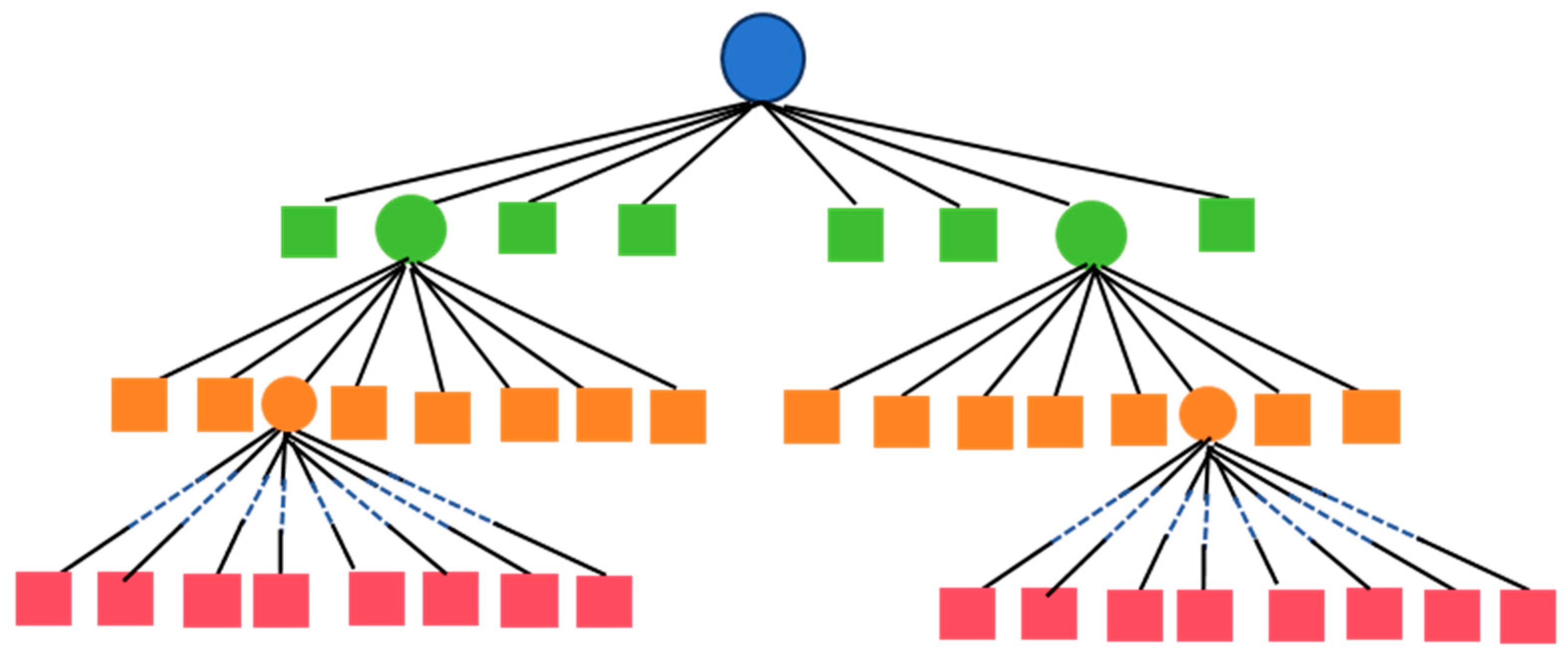
3.1. Grid Octree
3.2. Hard Coding Index
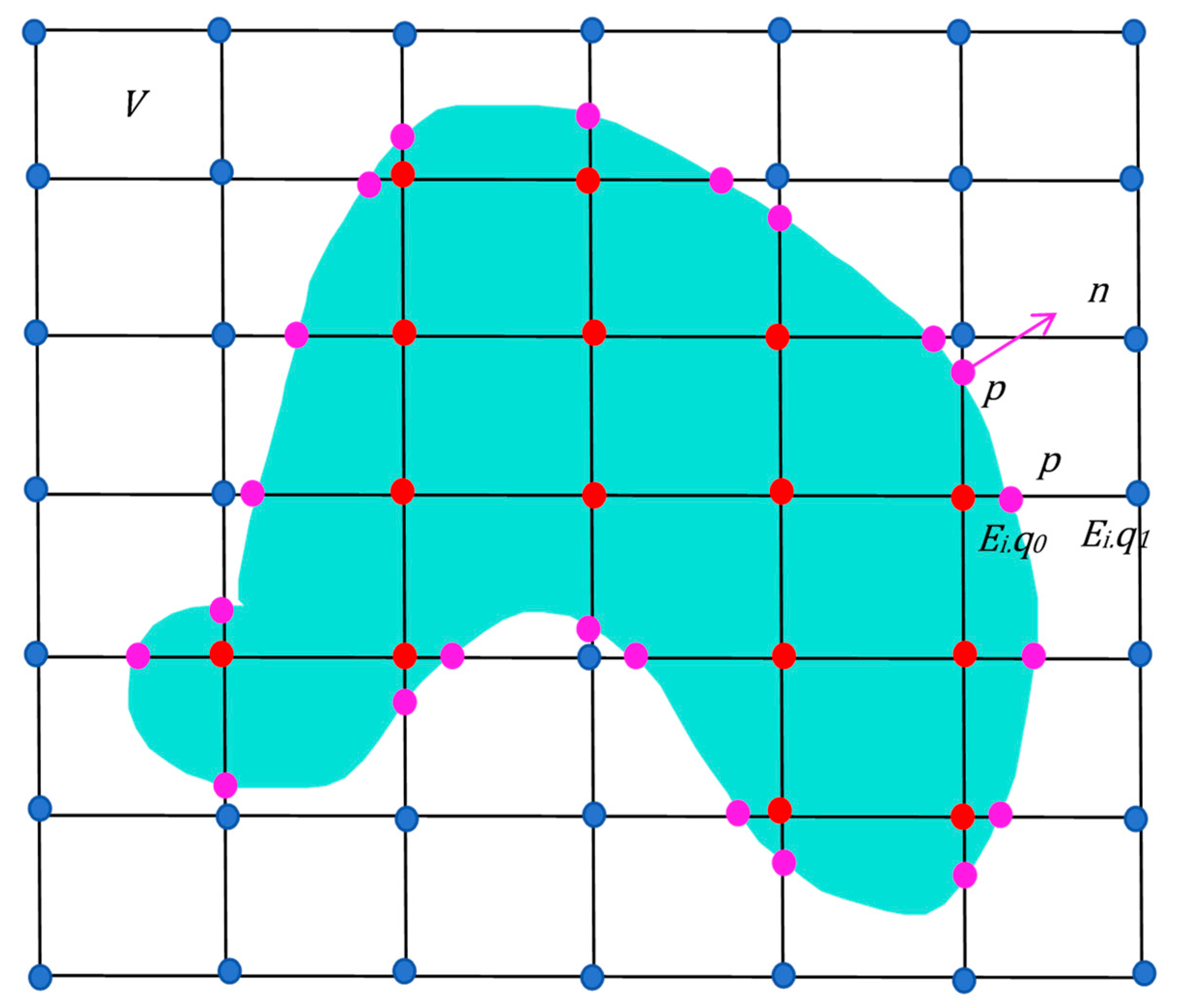
3.3. Voxel Fusion with Depth Map Interpolation
3.4. Mesh Extraction with Texture Constraints
4. Experiments and Results
4.1. Public Dataset
4.1.1. ICL-NUIM Dataset
4.1.2. TUM Dataset
4.2. Commercial 3D Scanner Data
4.2.1. Venus Model
4.2.2. Furniture
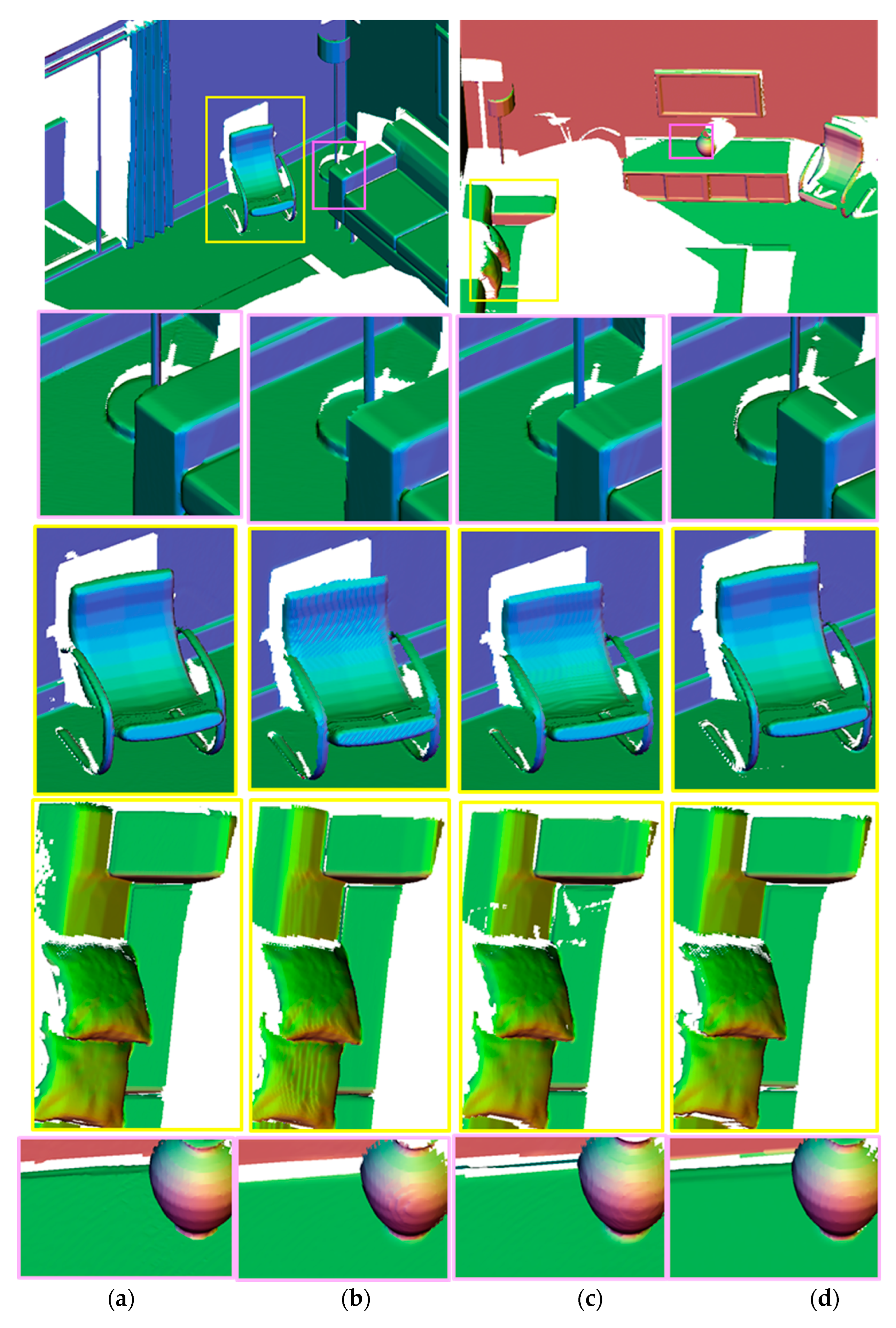
4.3. Surface Reconstruction Quality Evaluation and Analysis
4.4. Discussion
5. Conclusions
Author Contributions
Funding
Data Availability Statement
Conflicts of Interest
References
- Izadi, S.; Kim, D.; Hilliges, O.; Molyneaux, D.; Newcombe, R.; Kohli, P.; Shotton, J.; Hodges, S.; Freeman, D.; Davison, A. Kinectfusion: Real-Time 3D Reconstruction and Interaction Using a Moving Depth Camera. In Proceedings of the 24th Annual ACM Symposium on User Interface Software and Technology, Santa Barbara, CA, USA, 16–19 October 2011; pp. 559–568. [Google Scholar]
- Curless, B.; Levoy, M. A Volumetric Method for Building Complex Models from Range Images. In Proceedings of the 23rd Annual Conference on Computer Graphics and Interactive Techniques, New Orleans, LA, USA, 4–9 August 1996; pp. 303–312. [Google Scholar]
- Cao, Y.; Liu, Z.; Kuang, Z.; Kobbelt, L.; Hu, S. Learning to Reconstruct High-Quality 3D Shapes with Cascaded Fully Convolutional Networks. In Proceedings of the European Conference on Computer Vision (ECCV), Munich, Germany, 8–14 September 2018; pp. 616–633. [Google Scholar]
- Isler, S.; Sabzevari, R.; Delmerico, J.; Scaramuzza, D. An Information Gain Formulation for Active Volumetric 3D Reconstruction. In Proceedings of the 2016 IEEE International Conference on Robotics and Automation (ICRA), Stockholm, Sweden, 16–21 May 2016; pp. 3477–3484. [Google Scholar]
- Hinzmann, T.; Schönberger, J.L.; Pollefeys, M.; In Siegwart, R. Mapping on the Fly: Real-Time 3D Dense Reconstruction, Digital Surface Map and Incremental Orthomosaic Generation for Unmanned Aerial Vehicles. In Proceedings of the Field and Service Robotics: Results of the 11th International Conference, Zurich, Switzerland, 12–15 September 2017; Springer: Berlin/Heidelberg, Germany, 2018; pp. 383–396. [Google Scholar]
- Li, S.; Cheng, M.; Liu, Y.; Lu, S.; Wang, Y.; Prisacariu, V.A. Structured Skip List: A Compact Data Structure for 3D Reconstruction. In Proceedings of the 2018 IEEE/RSJ International Conference on Intelligent Robots and Systems (IROS), Madrid, Spain, 1–5 October 2018; pp. 1–7. [Google Scholar]
- Slavcheva, M.; Kehl, W.; Navab, N.; Ilic, S. SDF-2-SDF registration for real-time 3D reconstruction from RGB-D data. Int. J. Comput. Vision 2018, 126, 615–636. [Google Scholar] [CrossRef]
- Zheng, Z.; Yu, T.; Li, H.; Guo, K.; Dai, Q.; Fang, L.; Liu, Y. Hybridfusion: Real-Time Performance Capture Using a Single Depth Sensor and Sparse Imus. In Proceedings of the European Conference on Computer Vision (ECCV), Tel Aviv, Israel, 23–27 October 2018; pp. 384–400. [Google Scholar]
- Hornung, A.; Wurm, K.M.; Bennewitz, M.; Stachniss, C.; Burgard, W. OctoMap: An efficient probabilistic 3D mapping framework based on octrees. Auton. Robot. 2013, 34, 189–206. [Google Scholar] [CrossRef]
- Nießner, M.; Zollhöfer, M.; Izadi, S.; Stamminger, M. Real-time 3D reconstruction at scale using voxel hashing. ACM Trans. Graph. 2013, 32, 1–11. [Google Scholar] [CrossRef]
- Bylow, E.; Sturm, J.; Kerl, C.; Kahl, F.; Cremers, D. Real-Time Camera Tracking and 3D Reconstruction Using Signed Distance Functions. In Proceedings of the Robotics: Science and Systems (RSS) Conference 2013, Berlin, Germany, 24–28 June 2013. [Google Scholar]
- Newcombe, R.A.; Izadi, S.; Hilliges, O.; Molyneaux, D.; Kim, D.; Davison, A.J.; Kohi, P.; Shotton, J.; Hodges, S.; Fitzgibbon, A. Kinectfusion: Real-Time Dense Surface Mapping and Tracking. In Proceedings of the 2011 10th IEEE international Symposium on Mixed and Augmented Reality, Basel, Switzerland, 26–29 October 2011; pp. 127–136. [Google Scholar]
- Steinbrücker, F.; Sturm, J.; Cremers, D. Volumetric 3D Mapping in Real-Time on a CPU. In Proceedings of the 2014 IEEE International Conference on Robotics and Automation (ICRA), Hong Kong, China, 7 May–31 June 2014; pp. 2021–2028. [Google Scholar]
- Chen, J.; Bautembach, D.; Izadi, S. Scalable real-time volumetric surface reconstruction. ACM Trans. Graph. 2013, 32, 111–113. [Google Scholar] [CrossRef]
- Kähler, O.; Prisacariu, V.; Valentin, J.; Murray, D. Hierarchical voxel block hashing for efficient integration of depth images. IEEE Robot. Autom. Lett. 2015, 1, 192–197. [Google Scholar] [CrossRef]
- Fuhrmann, S.; Goesele, M. Fusion of depth maps with multiple scales. ACM Trans. Graph. 2011, 30, 1–8. [Google Scholar] [CrossRef]
- Dryanovski, I.; Klingensmith, M.; Srinivasa, S.S.; Xiao, J. Large-scale, real-time 3D scene reconstruction on a mobile device. Auton. Robot. 2017, 41, 1423–1445. [Google Scholar] [CrossRef]
- Vizzo, I.; Guadagnino, T.; Behley, J.; Stachniss, C. Vdbfusion: Flexible and efficient tsdf integration of range sensor data. Sensors 2022, 22, 1296. [Google Scholar] [CrossRef] [PubMed]
- Museth, K. VDB: High-resolution sparse volumes with dynamic topology. ACM Trans. Graph. 2013, 32, 1–22. [Google Scholar] [CrossRef]
- Oleynikova, H.; Taylor, Z.; Fehr, M.; Siegwart, R.; Nieto, J. Voxblox: Incremental 3d Euclidean Signed Distance Fields for On-Board Mav Planning. In Proceedings of the 2017 IEEE/RSJ International Conference on Intelligent Robots and Systems (IROS), Vancouver, BC, Canada, 24–28 September 2017; pp. 1366–1373. [Google Scholar]
- Vizzo, I.; Chen, X.; Chebrolu, N.; Behley, J.; Stachniss, C. Poisson Surface Reconstruction for LiDAR Odometry and Mapping. In Proceedings of the 2021 IEEE International Conference on Robotics and Automation (ICRA), Xi’an, China, 30 May–5 June 2021; pp. 5624–5630. [Google Scholar]
- Kazhdan, M.; Hoppe, H. Screened poisson surface reconstruction. ACM Trans. Graph. 2013, 32, 1–13. [Google Scholar] [CrossRef]
- Lorensen, W.E.; Cline, H.E. Marching cubes: A high resolution 3D surface construction algorithm. In Seminal Graphics: Pioneering Efforts that Shaped the Field; Association for Computing Machinery: New York, NY, USA, 1998; pp. 347–353. [Google Scholar]
- Dong, W.; Park, J.; Yang, Y.; Kaess, M. GPU Accelerated Robust Scene Reconstruction. In Proceedings of the 2019 IEEE/RSJ International Conference on Intelligent Robots and Systems (IROS), Macau, China, 3–8 November 2019; pp. 7863–7870. [Google Scholar]
- Dong, W.; Shi, J.; Tang, W.; Wang, X.; Zha, H. An Efficient Volumetric Mesh Representation for Real-Time Scene Reconstruction Using Spatial Hashing. In Proceedings of the 2018 IEEE International Conference on Robotics and Automation (ICRA), Brisbane, QLD, Australia, 21–26 May 2018; pp. 6323–6330. [Google Scholar]
- Hilton, A.; Stoddart, A.J.; Illingworth, J.; Windeatt, T. Marching Triangles: Range Image Fusion for Complex Object Modelling. In Proceedings of the 3rd IEEE International Conference on Image Processing, Lausanne, Switzerland, 19 September 1996; pp. 381–384. [Google Scholar]
- Sharf, A.; Lewiner, T.; Shklarski, G.; Toledo, S.; Cohen-Or, D. Interactive topology-aware surface reconstruction. ACM Trans. Graph. 2007, 26, 43. [Google Scholar] [CrossRef]
- Premebida, C.; Garrote, L.; Asvadi, A.; Ribeiro, A.P.; Nunes, U. High-Resolution Lidar-Based Depth Mapping Using Bilateral Filter. In Proceedings of the 2016 IEEE 19th International Conference on Intelligent Transportation Systems (ITSC), Rio de Janeiro, Brazil, 1–4 November 2016; pp. 2469–2474. [Google Scholar]
- Wu, C.; Zollhöfer, M.; Nießner, M.; Stamminger, M.; Izadi, S.; Theobalt, C. Real-time shading-based refinement for consumer depth cameras. ACM Trans. Graph. 2014, 33, 1–10. [Google Scholar] [CrossRef]
- Xie, W.; Wang, M.; Qi, X.; Zhang, L. 3D Surface Detail Enhancement from a Single Normal Map. In Proceedings of the IEEE International Conference on Computer Vision, Venice, Italy, 22–29 October 2017; pp. 2325–2333. [Google Scholar]
- Zhou, Q.; Neumann, U. 2.5D Dual Contouring: A Robust Approach to Creating Building Models from Aerial Lidar Point Clouds. In Proceedings of the Computer Vision—ECCV 2010: 11th European Conference on Computer Vision, Heraklion, Crete, Greece, 5–11 September 2010; Proceedings, Part III 11. Springer: Berlin/Heidelberg, Germany, 2010; pp. 115–128. [Google Scholar]
- Park, J.; Zhou, Q.; Koltun, V. Colored point cloud registration revisited. In Proceedings of the 2017 IEEE International Conference on Computer Vision (ICCV), Venice, Italy, 24–27 October 2017; pp. 143–152. [Google Scholar]
- Sturm, J.; Engelhard, N.; Endres, F.; Burgard, W.; Cremers, D. A Benchmark for the Evaluation of RGB-D SLAM Systems. In Proceedings of the IEEE/RSJ International Conference on Intelligent Robots and Systems, Vilamoura-Algarve, Portuga, l7–12 October 2012; pp. 573–580. [Google Scholar]
- Handa, A.; Whelan, T.; McDonald, J.; Davison, A.J. A Benchmark for RGB-D Visual Odometry, 3D Reconstruction and SLAM. In Proceedings of the 2014 IEEE International Conference on Robotics and Automation (ICRA), Hong Kong, China, 31 May–7 June 2014; pp. 1524–1531. [Google Scholar]
- Zhou, Q.; Park, J.; Koltun, V. Open3D: A modern library for 3D data processing. arxiv 2018, arXiv:1801.09847. [Google Scholar]
- Sommer, C.; Sang, L.; Schubert, D.; Cremers, D. Gradient-sdf: A Semi-Implicit Surface Representation for 3D Reconstruction. In Proceedings of the 2022 IEEE/CVF Conference on Computer Vision and Pattern Recognition (CVPR), New Orleans, LA, USA, 18–24 June 2022; pp. 6280–6289. [Google Scholar]


| ICL-NUIM | Voxel Size (0.01 m) | Truncation (3 Voxels) | ||
|---|---|---|---|---|
| Frame Rate | Memory Size | Disk Size | ||
| Open3D | 4.61 | 329.7 MB | 35.10 MB | |
| VDBFusion | 4.63 | 64 MB | 34.39 MB | |
| Gradient-SDF | 1.21 | 1293.2 MB | 25.94 MB | |
| RGBTSDF | 11.56 | 41.2 MB | 34.75 MB | |
| TUM | Voxel Size (0.01 m) | Truncation (8 Voxels) | ||
|---|---|---|---|---|
| Frame Rate | Memory Size | Disk Size | ||
| Open3D | 5.28 | 201.5 MB | 12.85 MB | |
| VDBFusion | 2.69 | 62.4 MB | 13.81 MB | |
| Gradient-SDF | 1.02 | 766.1 MB | 11.65 MB | |
| RGBTSDF | 15.22 | 29.9 MB | 12.74 MB | |
| Venus Model | Voxel Size (0.002 m) | Truncation (3 Voxels) | ||
|---|---|---|---|---|
| Frame Rate | Memory Size | Disk Size | ||
| Open3D | 2.15 | 1457.2 MB | 23.07 MB | |
| VDBFusion | 7.03 | 697.3 MB | 23.38 MB | |
| Gradient-SDF | 3.06 | 660.4 MB | 21.84 MB | |
| RGBTSDF | 19.72 | 325 MB | 23.84 MB | |
| Ornament of Guan Gong | Voxel Size (0.001 m) | Truncation (3 Voxels) | ||
|---|---|---|---|---|
| Frame Rate | Memory Size | Disk Size | ||
| Open3D | 1.45 | 2959 MB | 59.68 MB | |
| VDBFusion | 7.27 | 931.6 MB | 59.60 MB | |
| Gradient-SDF | 2.82 | 1367.6 MB | 57.26 MB | |
| RGBTSDF | 18.05 | 443.7 MB | 60.40 MB | |
Disclaimer/Publisher’s Note: The statements, opinions and data contained in all publications are solely those of the individual author(s) and contributor(s) and not of MDPI and/or the editor(s). MDPI and/or the editor(s) disclaim responsibility for any injury to people or property resulting from any ideas, methods, instructions or products referred to in the content. |
© 2024 by the authors. Licensee MDPI, Basel, Switzerland. This article is an open access article distributed under the terms and conditions of the Creative Commons Attribution (CC BY) license (https://creativecommons.org/licenses/by/4.0/).
Share and Cite
Li, Y.; Huang, S.; Chen, Y.; Ding, Y.; Zhao, P.; Hu, Q.; Zhang, X. RGBTSDF: An Efficient and Simple Method for Color Truncated Signed Distance Field (TSDF) Volume Fusion Based on RGB-D Images. Remote Sens. 2024, 16, 3188. https://doi.org/10.3390/rs16173188
Li Y, Huang S, Chen Y, Ding Y, Zhao P, Hu Q, Zhang X. RGBTSDF: An Efficient and Simple Method for Color Truncated Signed Distance Field (TSDF) Volume Fusion Based on RGB-D Images. Remote Sensing. 2024; 16(17):3188. https://doi.org/10.3390/rs16173188
Chicago/Turabian StyleLi, Yunqiang, Shuowen Huang, Ying Chen, Yong Ding, Pengcheng Zhao, Qingwu Hu, and Xujie Zhang. 2024. "RGBTSDF: An Efficient and Simple Method for Color Truncated Signed Distance Field (TSDF) Volume Fusion Based on RGB-D Images" Remote Sensing 16, no. 17: 3188. https://doi.org/10.3390/rs16173188