Article

Evaluating the Performance of Pulsed and Continuous-Wave Lidar Wind Profilers with a Controlled Motion Experiment

by
Shokoufeh Malekmohammadi
1,*,
Christiane Duscha
1,
Alastair D. Jenkins
1,
Felix Kelberlau
2,
Julia Gottschall
3 and
Joachim Reuder
1
1
Geophysical Institute and Bergen Offshore Wind Centre (BOW), University of Bergen, 5007 Bergen, Norway
2
Fugro Norway AS, 7462 Trondheim, Norway
3
Fraunhofer Institute for Wind Energy Systems (IWES), 27572 Bremerhaven, Germany
*
Author to whom correspondence should be addressed.
Remote Sens. 2024, 16(17), 3191; https://doi.org/10.3390/rs16173191 (registering DOI)
Submission received: 22 July 2024 / Revised: 23 August 2024 / Accepted: 26 August 2024 / Published: 29 August 2024
(This article belongs to the Special Issue Observation of Atmospheric Boundary-Layer Based on Remote Sensing)

Abstract

:
While floating wind lidars provide reliable and cost-effective measurements, these measurements may be inaccurate due to the motion of the installation platforms. Prior studies have not distinguished between systematic errors associated with lidars and errors resulting from motion. This study will fill this gap by examining the impact of platform motion on two types of profiling wind lidar systems: the pulsed WindCube V1 (Leosphere) and the continuous-wave ZephIR 300 (Natural Power). On a moving hexapod platform, both systems were subjected to 50 controlled sinusoidal motion cases in different degrees of freedom. Two reference lidars were placed at a distance of five meters from the platform as reference lidars. Motion-induced errors in mean wind speed and turbulence intensity estimation by lidars are analyzed. Additionally, the effectiveness of a motion correction approach in reducing these errors across various scenarios is evaluated. The results indicate that presence of rotational motion leads to higher turbulence intensity (TI) estimation by moving lidars. The absolute percentage error between lidars is the highest when lidars are exposed to yaw and heave motion and is the lowest when exposed to surge motion. The correlation between lidars, though it is the lowest in the presence of pitch, yaw, and heave motion. Furthermore, applying motion compensation can compensate the correlation drop and erroneous TI estimation.

1. Introduction

Accurate offshore wind condition observations are essential for proper wind resource assessment during wind farm planning and design. These observations are also critical for optimizing wind farm operation and control. It is also crucial for the characterization of appropriate weather windows required for marine operations related to turbine installation, maintenance, and repair in the marine environment. Yet, wind observations at offshore sites are sparse, leaving the characterization of the flow field in and around offshore wind farms as one of the big challenges for its future large-scale deployment [1]. Traditionally, mast-mounted anemometers have been used for corresponding measurements such as, e.g., the German FINO research platforms in the North and Baltic seas [2], or the Ilmujden mast off the Dutch coast [3]. Such mast-based measurements are, however, very expensive, logistically demanding, and restricted to a single location and thus lack flexibility. In addition, masts are infeasible for acquiring wind speed data over the rotor disc of modern wind turbines, now exceeding 250 m [4].
Wind lidars have emerged as a reliable and cost-effective alternative to conventional meteorological masts for comprehensive wind field monitoring [5,6]. They have specific advantages, in particular offshore, where met masts cannot be deployed in a cost-effective way [7]. Consequently, lidar systems have been deployed offshore in diverse setups, depending on the corresponding measurement goals, including mounting on wind turbine nacelles [8,9,10], on fixed platforms like research platforms, electrical sub-stations or bottom-fixed turbines [11,12,13], and on dynamic platforms such as vessels or buoys [14,15,16,17,18]. When positioned on static platforms, such lidars effectively reach altitudes aligning with the size of modern turbines. However, their placement is again stationary and constrained to the foundation location. Therefore, deploying wind lidars on dynamic platforms, such as ships, can be a promising solution to overcome the limitations associated with their static counterparts [14,19,20,21,22].
The deployment of wind profiling lidars on a floating platform causes inevitable challenges related to motion-induced errors in the retrieval of wind speed and direction [17,23,24,25,26,27]. The corresponding floating lidar systems (FLS) are exposed to wave-induced rotational and, in particular for ship-mounted systems, also considerable translational motion. The latter ones (heave, surge, and sway) directly superimpose artificial relative speeds, while the angular motions (pitch, roll, and yaw) are constantly altering the measurement geometry and thus affecting and complicating the wind field reconstruction required to derive horizontal wind speed and direction from multiple line-of-sight (LOS) readings. The amplitude of the resulting motion-induced errors depends on the lidar type (pulsed vs. continuous wave); the chosen measurement geometry and sampling frequency; the speed, frequency, and amplitude of the applied motion; and the chosen averaging interval [27]. Previous research has shown that the motion-induced errors in 10 min mean wind speed only range from 1% to 2% [14], as the effects of the random motion by the waves with periods in the order of 0.1 Hz are averaged out. Thus, 10 min average wind retrievals from FLS might provide sufficient accuracy for, e.g., resource assessment, even without any motion correction. The quality in the derivation of other important design parameters, such as the turbulence intensity (TI), defined as the standard deviation of the instantaneous wind measurements divided by the mean value, will in contrast be highly affected by the motion. Consequently, proper measures for motion compensation or motion correction are required to correct motion-induced errors on the instantaneous wind measurements.
One approach to mitigate the motion effects is the utilization of mechanical compensation systems, where the lidar is operated on actively or passively stabilized instrument platforms [15,23,28,29]. Size, weight, and energy constraints make this form of motion compensation, however, infeasible for many buoy-based applications. Therefore, motion correction algorithms were developed and applied to FLS data during the post-processing stage [18,20,25,30]. The testing and validation of the efficiency of the corresponding compensation algorithms requires systematic experimental efforts. As highlighted in Thebault et al. [31] and Kelberlau and Mann [27], systematic and controlled motion experiments are to date very scarce. Only a controlled setup of co-located moving and stationary lidar wind profilers allows distinguishing between the motion-induced errors in lidar measurements and potential systematic and random errors arising from the lidar measurement principle, setup, or the atmospheric conditions during the measurements.
This manuscript addresses this research gap by detailing and presenting a controlled-motion lidar experiment conducted in August 2011 at the campus of the University of Agder in Grimstad, Norway. In this experiment, two different types of profiling wind lidar systems, the pulsed WindCube V1 (manufactured by Leosphere, France) and the continuous-wave (CW) ZephIR 300 (manufactured by Natural Power, UK) were installed on a 6 degree-of-freedom (DOF) hexapod motion platform and exposed to 55 different controlled motion test cases. Two fixed-reference lidars of corresponding types were positioned 5 m from the platform. Most of the test cases were characterized by sinusoidal motion (in one or two degrees of freedom) with constant amplitude and frequency. The collected data from this experiment are analyzed statistically, highlighting the impact of various motion patterns and characteristics on measurements of mean wind speed and estimation of turbulence intensity. In addition, the performance of novel motion correction approaches to reduce the motion-induced error in various motion scenarios is evaluated.

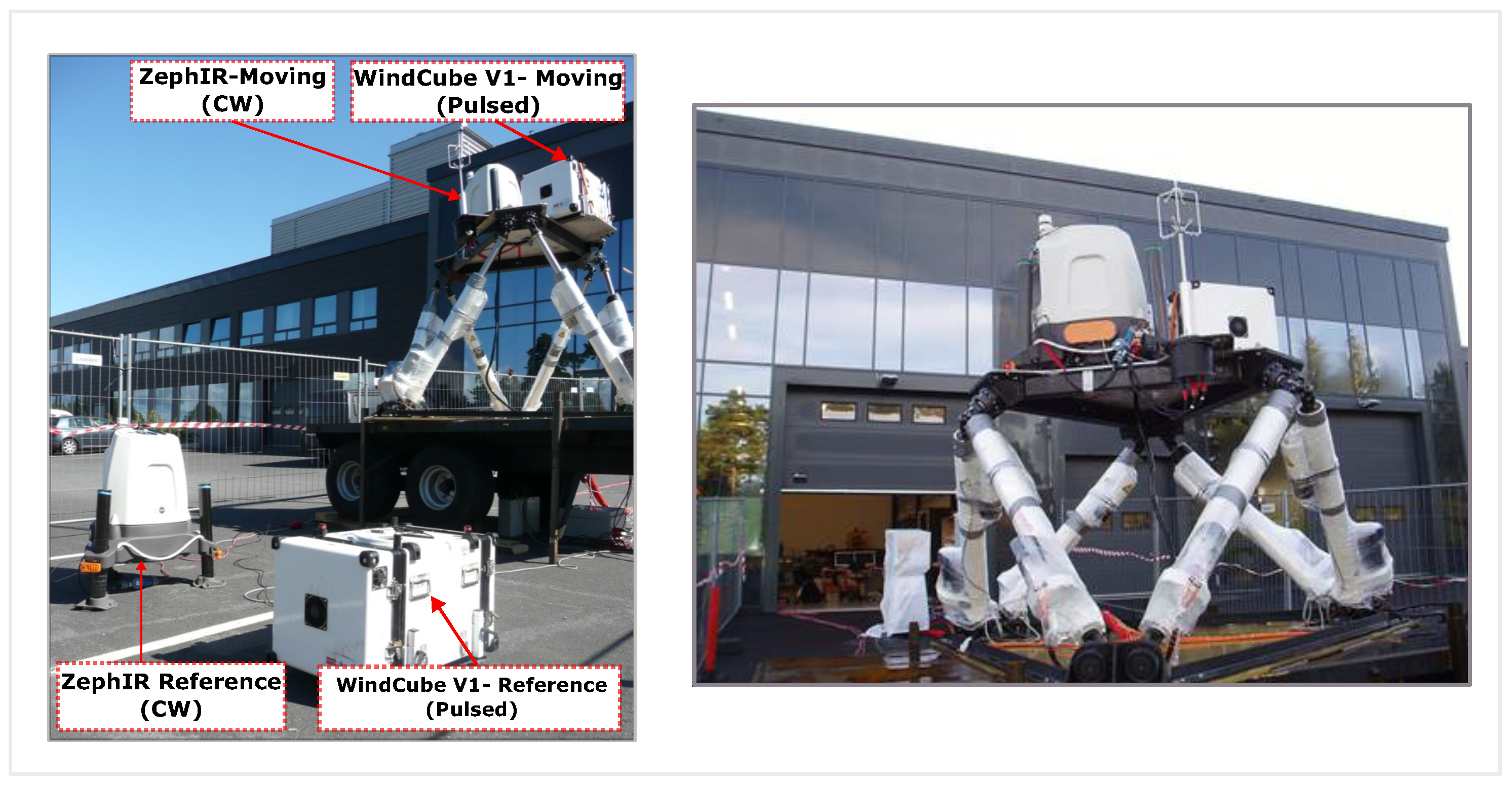
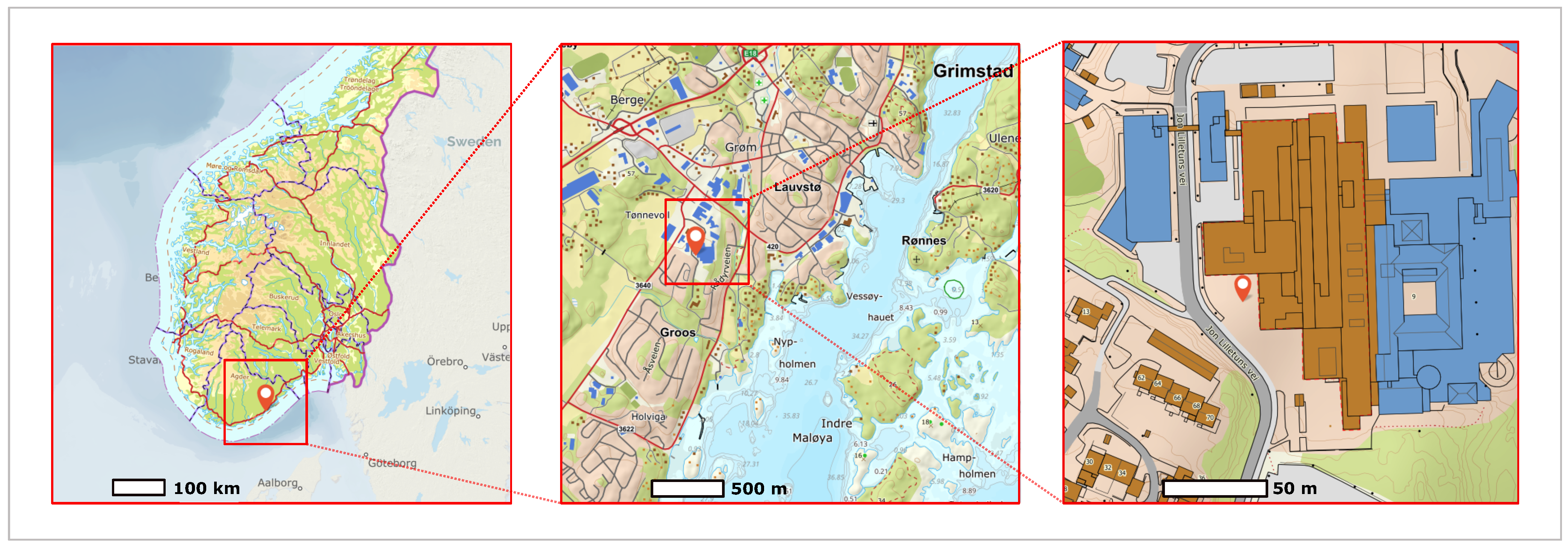
2. The Grimstad Experiment—Site Specifications

The experiment was conducted at the Grimstad campus of the University of Agder, Southern Norway, over a ten-day period. Due to practical and logistical considerations, such as the length of power and control cables and the motion platform not being certified for outdoor operation, in particular in rain, the test site had to be located near the laboratory building of the University. This building is approximately nine meters in height, and the motion platform was located approximately ten meters west of it, with the reference lidars located approximately five meters further west (see Figure 1). The overall topography of the site at the university campus is relatively flat within a radius of one kilometer, with the sea to the South and East and some more hilly terrain towards the West (Figure 2).
Two types of lidar wind profilers, a pulsed system, WindCube V1 (manufactured by Leosphere, France), and a CW system, ZephIR 300 (manufactured by Natural Power, Malvern, UK), were deployed in the experiment. One instrument of each type was mounted on a motion platform (hereafter referred to as moving lidars) and exposed to several controlled motion patterns with constant frequency f 0 and amplitude A 0 . The motion platform used at this experiment was a 6-DOF E-motion 1500 Motion System (manufactured by Bosch Rexroth, Boxtel, Netherlands). Two corresponding fixed reference lidar systems were located at a distance of 5 m from the platform. The coordinates of the lidars were defined such that the X axis was pointing south, the Y-axis was pointing west, and the Z-axis was pointing down.
The experiment began on 2011-08-16 at 15:50 and ended on 2011-08-25 at 17:50 UTC. A total of 55 test cases were applied to the lidars to investigate the effect of various motion types on the lidars’ performance (including roll, pitch, yaw, heave, and surge in addition to combined motions, see Table A1). The number of test cases was primarily determined by the availability of the motion platform, which was limited to a two-week period. During this time, the objective was to conduct a comprehensive series of tests that included both individual and combined motion scenarios to systematically investigate the effects of motion on lidar systems. Furthermore, each motion scenario was sustained for a sufficient duration (typically three hours) to ensure a robust statistical analysis.
For each test case, the lidars on the moving platform were subjected to a specific motion. Throughout the experiment, the moving lidars were kept stationary during nighttime to allow for a baseline comparison of the systems in non-moving conditions. As reported in the experiment log, some of the baseline test cases were ineffective because of either a lack of data or a malfunctioning lidar at the time of the baseline tests (tests 7, 18 and 30); thus, these tests have been discarded from the analysis.
The lidars were set to measure wind speed up to 200 m above the surface at 10 different heights. Table A2 shows the height settings for the four lidars during tests 1 to 10. As a correction for the difference in height between the neutral position of the motion platform mounting plate and the ground, a 3 m offset has been subtracted from the height setting of the moving lidars. WindCube V1 demonstrated the best signal levels and accuracy at about 85 m. Hence, from test 11, ZephIR 300 lidars were configured to measure at 85 m eight times, at 45 m once, and at 145 m once for a more reliable statistical basis at 85 m (see Table A3). Therefore, in this study, the data will be evaluated at 85 m and also 145 m as a reference height for modern wind turbines. The motion data were recorded by a six-DOF Cross-Box—NAV440 inertial measurement unit (IMU).

3. Lidar Theory

The vertical profiling wind lidars that were used in this study, measure wind speed up to 300 m. In profiling lidars, a laser beam is emitted at a fixed elevation angle ϕ and at several azimuth angles α (see Figure 3), with the number of azimuth angles varying based on the type of lidar.
The WindCube V1 emits a sequence of pulsed lasers beams in four azimuth angles (0°, 90°, 180°, 270°) in a Doppler-beam swinging (DBS) scanning pattern. This system simultaneously measures wind at several predetermined heights. The ZephIR 300 lidar, also referred to as ZX300, performs a velocity azimuth display (VAD) scanning pattern. Here, the lidar transmits a continuous wave (CW) laser beam at 50 different azimuth angles at a fixed height. The beam intercepts the wind at different angles as it moves, building up a series of measurements around a cone that can be used to retrieve the wind velocity vector. After completing one VAD scan, the laser is refocused on the next height. Both lidars have a cone half-opening angle or zenith angle θ approximately 30 ° .
The LOS velocity, v r , observed by the lidar for a specific θ , and α , is linked to the wind velocity vector u = ( u , v , w ) by
v r = u cos α sin θ + v sin α sin θ + w cos θ ,
as explained in [32]. At least three independent LOS velocities are required to reconstruct one wind vector using Equation (1). The pulsed lidar WindCube V1 emits beams at four azimuth angles. In one cycle of the DBS scan, the following radial velocities are observed:
v r ( α = 0 ° ) v r ( α = 90 ° ) v r ( α = 180 ° ) v r ( α = 270 ° ) = sin θ 0 cos θ 0 sin θ cos θ sin θ 0 cos θ 0 sin θ cos θ u v w ,
which can also be written as
v r = N u .
This system of equations can be solved analytically when only three radial velocity measurements are considered. In cases where the system is over-determined, the least-squares fitting method can be used.
For ZephIR 300, at each VAD scan, horizontal wind speed u h o r , vertical speed w, and direction Θ are extracted from
v r = | A cos ( α B ) + C | ,
where A = u h o r sin θ , B = Θ or B = Θ ± 180 ° , and C = w cos θ . The solution for B reflects the ambiguity issue in continuous-wave wind lidars, where the system cannot distinguish wind direction. We add or subtract 180° to ensure the solution remains within the range of 0–360°. Equation (4) can be solved by finding the best fit using the least squares approach [18,33].

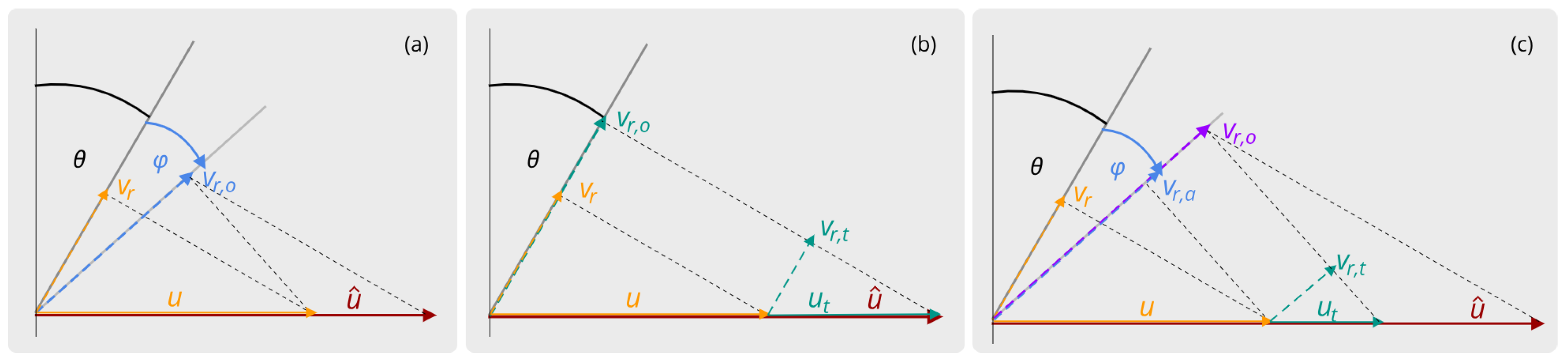
Motion Effect on Lidar Measurements

On a moving platform such as a buoy or ship, the lidar is subjected to motion in six DOF: rotational motion (roll β , pitch φ , and yaw ψ ) around the x, y, and z axes and translational motion (surge, sway, and heave) along the x, y, and z axes, respectively. This motion affects the observed v r values and the velocity vector resulting from retrieval ( u ^ ). If the lidar experiences rotational motion in one DOF, such as rotation around the y axis, the beam orientation along the x-axis is altered by φ (Figure 4a); therefore, the observed LOS velocity changes from u sin ( θ ) to u sin ( θ + φ ) .
As the standard wind vector retrieval uses the beam projection based on θ instead of θ + φ , the retrieved wind vector will be erroneous.
Further, if the lidar experiences translational motion in one DOF, such as along the x axis ( u t ), the observed LOS velocity changes from u sin ( θ ) to u sin ( θ ) + u t sin ( θ ) . Consequently, u ^ changes (see Figure 4b). In a combination of rotational and translational motion (Figure 4c), both u and u t are projected onto the rotated beam, changing u sin ( θ ) to u sin ( θ + φ ) + u t sin ( θ + φ ) .
Thus, if the lidar is impacted by motion, Equation (3) changes to
v r = RN ( u + u T ) ,
with the translational motion vector u T and the rotation matrix R, constructed from the rotation matrices Rx, Ry, and Rz corresponding to roll ( β ), pitch ( φ ), and yaw ( ψ ) of the inertial coordinate system:
R x = 1 0 0 0 cos β sin β 0 sin β cos β , R y = cos φ 0 sin φ 0 1 0 sin φ 0 cos φ , R z = cos ψ sin ψ 0 sin ψ cos ψ 0 0 0 1 .

4. Methods

4.1. Motion Correction

To correct the motion-induced errors on the lidar measurements, the pitch, roll, and yaw angles, as well as the translational velocities, are obtained from an IMU. In addition, the LOS velocities are obtained directly from the lidar. These measurements are utilized to reconstruct the motion-corrected wind vectors by solving the equation system (Equation (5)) for u using the least squares approach:
u ^ = [ ( RN ) T RN ] 1 ( RN ) T ( v r v r T ) ,
where v r T = RN u T . For a comprehensive explanation of this approach as applied to the ZephIR 300, we refer readers to Kelberlau et al. [18].

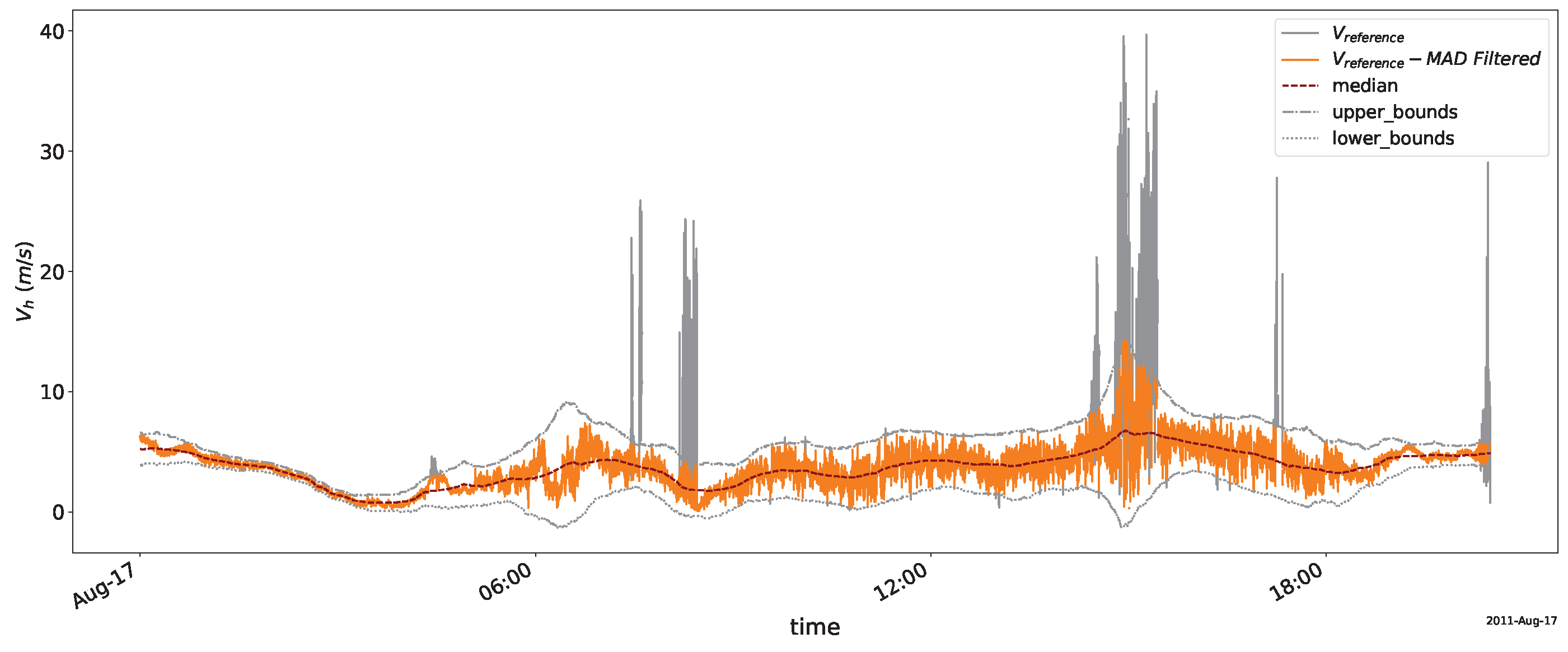
4.2. Data Filtering and Statistical Methods

For the duration of the experiment, the Norwegian hindcast archive (NORA3) results never showed a wind speed exceeding 20 ms−1. Thus, lidar measurements exceeding 20 ms−1 were considered nonphysical and flagged as not a number (NaN). The NORA3 utilizes the HARMONIE-AROME numerical weather prediction model to offer a reanalysis of atmospheric data. This reanalysis features a spatial resolution of 3 km and a temporal resolution of 1 h [34].
Furthermore, three steps were taken to filter the data. Firstly, low-quality signals were discarded. To discard the low-quality signals, line-of-sight (LOS) velocities with carrier-to-noise ratios (CNRs) less than −23 dB were excluded from the analysis. This threshold value is suggested by manufacturer and is chosen based on the analysis of Pearson et al. [35].
Secondly, the outliers were detected and discarded using the median absolute deviation (MAD) approach [36,37]. Any observation (X) is considered an outlier if
| X M | > 3 × M 0.6745 ,
where M is the rolling median of all observations. The wind speeds measured by the WindCube V1 reference on 2011-08-17 at 85 m before (gray) and after (orange) applying the MAD filter are shown in Figure 5 as an example. This visualization illustrates the effectiveness of the MAD method in removing high spikes in the raw data. Yet, some spikes in wind speed are present in the time series of the WindCube V1 reference (see Figure 5 at 15:00 UTC).
In the experiment log, it was reported that the WindCube V1 reference occasionally overestimated wind speed due to unresolved technical issues. This might be the reason for the presence of such erroneous spikes in the WindCube V1 reference data. These data were considered faulty and non-physical.
To identify and discard these faulty data in the WindCube V1 reference data, the third step in filtering was taken. In this step, comparisons were made between the moving and reference lidar of each type, constraining the relative difference of their standard deviations to 70% to ensure measurement consistency. The relative standard deviation was defined as
Δ σ relative = σ ref σ moving 1 ,
where σ ref is the standard deviation of the WindCube V1 reference data and σ moving is the standard deviation of the WindCube V1 moving data. The latter was considered as the base for the filtering. Using this measure, the data points of the WindCube V1 reference with a Δ σ relative exceeding 70% were excluded from analysis. This ensures that the standard deviation of the reference lidar does not exceed the standard deviation of the moving lidar by more than 70%. As in the ZephIR300 data, such inconsistency was not observed, only the first two steps were applied to the data.
After filtering the data, all test cases which had data availability of less than 50% were discarded. Wind speeds at the two heights of 85 m and 145 m were then obtained from the lidars without motion correction. As an initial survey, the performance of the lidars was compared based on the baseline test cases. Later on, the lidars’ performances based on the motion type were compared. The turbulence intensity (TI) estimate of lidars was calculated as
TI = σ U U ¯ ,
where σ U represents standard deviation of horizontal wind speed and U ¯ represents the mean wind speed within the test time span. Here, the TI is an estimation of turbulence intensity using the lidar measurements and is different from the actual TI conventionally used in wind energy community [14,18,26]. The absolute percentage error (APE) measuring the absolute difference between the reference and moving lidars was calculated for each type of lidars at each test case as
APE = U ¯ r e f e r e n c e U ¯ m o v i n g U ¯ r e f e r e n c e × 100 .
The Pearson correlation coefficient was also calculated to quantify the degree of agreement between measurements obtained from the moving and reference lidar systems of each type. Using the motion data obtained from the IMU, the motion correction algorithm explained in Section 3 was applied to the moving lidar data. The corrected data were then compared to reference lidar data.

5. Results

In Figure 6, the average wind speed and estimated TI measured by lidars at 85 m and 145 m heights, along with test case numbers, are shown. Orange bars represent the ZephIR 300 results, while blue bars correspond to WindCube V1 results. Darker shades indicate measurements from moving lidars, and lighter shades indicate measurements from reference lidars. In addition, Figure 7 shows the APE between moving and reference lidars for each type at Figure 7a,b and the corresponding correlations are shown in Figure 7c,d.

5.1. Lidars’ Performance with No Motion: Baseline Test Cases

The baseline measurements are shown in the first row of Figure 6. In general, the mean wind speeds are consistent across most tests, with one exception in test 02. During this particular test, WindCube V1 recorded an average wind speed that is twice as high as that measured by the ZephIR 300, at both heights. However, for the majority of tests, the wind speeds recorded by both lidar systems are comparable. The TI estimated by ZephIR 300 is slightly higher than that of WindCube V1. The APEs of lidars in the baseline test cases are less than 2% for both types at 85 m, while this difference exceeds 5% for WindCube V1 at 145 m. Correlation between the two lidars of each type at two heights is more than 0.90 for all test cases. This high correlation suggests that the relative trends and patterns captured by both lidar systems is consistent. Therefore, the non-moving lidars serve as reliable sources of reference data for subsequent test cases.

5.2. Lidars’ Performance in Presence of the Motion

5.2.1. Rotational Motion: Yaw (Rotation along Z Axis)

The statistical analysis of lidar data during yaw motion (tests 19, 20, 21, 48, and 49) is shown in the second row of Figure 6. All of the above test cases have similar amplitudes ( A 0 = 39 ° ), but different frequencies ( f 0 ) see Table A1. The moving lidars have a lower average wind speed than the reference ones except in test 49 for both WindCube V1 and ZephIR 300. In test 48, ZephIR 300 moving has slightly higher mean wind speeds (Figure 6 Yaw: a, b). Additionally, the WindCube V1 pair’s TI estimates are lower than those of ZephIR, except in test 49 (Figure 6 Yaw: c, d). Interestingly, the moving ZephIR 300 estimates less TI than the reference ZephIR 300 in the majority of cases. The APE is higher for WindCube V1, exceeding 14%, while ZephIR 300 has a maximum of 5% APE (Figure 7 Yaw: a, b). The highest APE is observed in test cases with high frequencies. Furthermore, the correlation between the moving and reference lidars varies greatly, ranging from 0.28 to 0.86. The lowest correlation occurs in test 49 with a 0.25 Hz frequency, while the highest correlation occurs in test 21 with f 0 = 0.05 Hz (Figure 7 Yaw: c, d).

5.2.2. Rotational Motion: Pitch (Rotation along N–S)

The statistical analysis of lidar data during pitch motion (tests 8, 9, 10, 11, 52, and 55) is shown in the third row of Figure 6. Across these tests, pitch amplitudes ranged from 3° to 20° and f 0 from 0.1 to 0.2 Hz. In this type of motion, the lidars consistently measure similar mean wind speeds, but vary significantly in turbulence intensity (TI) estimation. Generally, the WindCube V1 exhibits higher TI estimates than the ZephIR 300 for both moving and reference lidars. Specifically, tests 10, 11, and 52 have the largest TI discrepancies between the moving and reference lidars, coinciding with higher pitch amplitudes (10°, 15°, 20°) and frequency (0.2 Hz). The value of TI for test 10, however, is the lowest, likely due to higher mean wind speeds where wind speed fluctuations are typically lower.
The APE remains below 2.5% for both lidar types at the height of 85 m (Figure 7 Pitch: a), whereas WindCube V1 shows a considerable increase in APE at 145 m (Figure 7 Pitch: b). The correlation between moving and reference lidars during this motion consistently exceeds 0.75. Interestingly, in tests with higher pitch amplitudes (such as tests 10, 11, and 52), the correlation decreases significantly for WindCube V1 lidars, while the ZephIR 300 ones maintain a higher level of correlation. Given the similarity in motion frequencies and the increase in motion amplitude only, it can be inferred that pitch motion amplitude likely plays a predominant role in motion-induced errors. When considering the motion pattern in conjunction with the lidar’s conical scanning shape, it is possible to understand how increasing the motion amplitude would affect the lidar’s scanning pattern. There is a detailed discussion of this alteration in [18,27]. Our observations confirm the results of [27], which show that the pitch motion-induced error depends strongly on motion amplitude.

5.2.3. Rotational Motion: Roll (Rotation along E–W)

The statistical analysis of lidar data during roll motion (tests 12, 22, 23, and 51) can be seen in the fourth row of Figure 6. Test cases 12, 22, and 23 have motion frequencies of 0.2 Hz and amplitudes of 15°, 10°, and 5°. In test 51, where f 0 = 0.1 Hz and A 0 = 15 ° , the moving WindCube V1 exhibits a slightly lower average wind speed across all tests when compared to the reference WindCube V1. However, the moving lidar has higher TI, indicating increased measurement fluctuations due to lidar motion. For the ZephIR 300 lidars, moving lidar also has a lower average wind estimation, yet the TI estimations are less different when compared to the WindCube V1 estimates except for test 51. The test cases 12, 22, 23 only differ in motion amplitude and have higher frequency than test 51. Interestingly, the TI in these test cases is lower than test 51.
The APE for WindCube V1 is less than ZephIR 300 at 85 m and this value for both lidars remains less than 2.5%, except for test 51 in which WindCube V1 shows an APE higher than 5%. While the APE for ZephIR 300 remains at around 2.5% at 145 m, this value for WindCube V1 reaches 7% (Figure 7 Roll: a, b). The correlation between the lidars in Figure 7 (Roll: c, d) indicate that the ZephIR 300 lidars are reasonably correlated, even with the presence of the motion except for test 51, while the correlation of WindCube V1 is affected more and decreases at 145 m.

5.2.4. Vertical Motion along Z Axis (Heave)

The statistical analysis of lidar data during heave motion (tests 3, 4, 5, 36, 38, and 56) is presented in the fifth row of Figure 6. The moving lidars were subjected to vertical displacements with f 0 ranging from 0.1 Hz to 0.4 Hz. Test cases 03, 36, and 38 have A 0 = 40 cm. The mean wind speeds measured by the moving lidars were similar to or slightly lower than those measured by the reference lidars at both heights, except for test 56, which showed a large discrepancy between the reference and moving ZephIR 300 (Figure 6 Heave: a, b).
In terms of TI estimation, WindCube V1 lidars displayed a noticeable discrepancy between moving and reference measurements, whereas ZephIR 300 showed similar TI estimations (Figure 6 Heave: c, d). The APE between moving and reference lidars reached 5% at 85 m for WindCube V1 and was less than 3% for ZephIR 300. At 145 m, the APE remained below 2% for ZephIR 300 but reached 24.3% for WindCube V1, which is a considerable amount (Figure 7 Heave: a, b). The correlation between the lidars varied from 0.9 in test 3 to 0.2 in test 36. Correlation was consistently lower at 145 m for all test cases. As motion frequency increased, the correlation of WindCube V1 lidars decreased, while the correlation of ZephIR 300 increased (Figure 7 Heave: c, d).

5.2.5. Horizontal Motion along N–S Axis (Surge)

The statistical analysis of lidar data during surge motion (tests 6, 31, and 54) is presented in the last row of Figure 6. The lidars were subjected to sinusoidal oscillations with A 0 = 40 cm. For test 6 and 31 f 0 = 0.1 Hz, and for test 54 f 0 = 0.2 Hz. All lidars measured similar mean wind speeds, with slight overestimation by the WindCube V1 reference (Figure 6 Surge: a, b). Moreover, moving lidars exhibited higher TI estimates at 85 m compared to reference lidars. Additionally, WindCube V1 consistently showed higher TI estimates than ZephIR 300, indicating greater variability in WindCube V1 measurements (Figure 6 Surge: c, d). Strong linear relationships between moving and corresponding reference lidars were observed, with correlation values ranging from 0.73 to 0.90 in Figure 7 (Surge: c, d). However, correlations were lower at 145 m compared to 85 m. The APE between the WindCube V1 moving and reference lidars was less than 2.5% at 85 m and 7.5% at 145 m, whereas for ZephIR 300, the APE was below 2.5% at both heights (Figure 7 Surge: a, b). Our findings suggest that surge motion had negligible effects on the ZephIR 300 measurements, while WindCube V1 showed increased susceptibility to motion-induced errors at higher heights. However, due to the limited range of frequencies and the small number of test cases available here, definitive conclusions cannot be drawn.

5.3. Discussion of the Observed Motion-Induced Errors

Kelberlau and Mann [27] showed that the tilt of lidars can cause degrees of error varying from no error to very large errors in measurements depending on factors such as the lidar’s sampling frequency (the frequency of completing a VAD scan f s ), the amplitude of the motion, the presence of wind shear, and the wind direction. It is important to note that their study defines roll and pitch motions as the tilt of the lidar in the along-wind and crosswind directions, respectively. We, however, define the tilt rotations according to the geographic coordinate system. Consequently, we do not anticipate the roll rotation in the absence of wind shear to result in zero error and pitch to cause the highest errors as demonstrated in [27]. Nevertheless, we can explain our findings in light of their simulation results by considering both roll and pitch test cases as the tilt of the lidar, which may or may not correspond to the along-wind rotation.
If the f 0 < f s , the scanning cone is tilted completely in one cycle of motion, and hence the scanning geometry can be considered frozen, maintaining a consistent scanning geometry. Consequently, here test cases with f 0 = 0.1 , 0.2 Hz are considered slow tilts for the ZephIR 300 with f s = 1 Hz and the error is expected to increase only with increasing amplitude [27]. We expect test case 22 to result in lower errors compared to tests 23 and 12 (due to increased amplitude) of around 1.5%, and test 51 to cause the highest error of around 2%, based on Figure 6 in [27].
For WindCube V1 with f s = 0.25 Hz, tilts with an f 0 between 0.1 and 0.2 Hz are anticipated to cause higher errors, as f 0 f s . For instance, test 11 with A 0 = 15 ° and f 0 = 0.2 Hz as well as test 23 are expected to result in the highest errors, around 4% [27]. This aligns closely with the APE values measured by the WindCube V1 in our observations (see Figure 7). However, at 145 m, the APE is considerably higher, likely due to system differences which are even present in the absence of motion (baseline test cases). Furthermore, the presence of wind shear is expected to cause a tilted lidar to underestimate wind speed [27]. In all of our test cases with roll motion, wind shear is evident, particularly in tests 22 and 23. This explains the underestimation of mean wind speed measured by the moving lidars for both types.
Regarding the yaw motion, Kelberlau and Mann [27] have only explored the effect of slow yaw motion on lidars, finding it to be negligible. This is consistent with the behavior observed in the ZephIR 300 during our experiment with f s = 1 Hz and yaw motion frequencies ranging from 0.025 to 0.2 Hz. However, the WindCube V1, with its lower sampling frequency ( f s = 0.25 Hz), might exhibit greater errors due to yaw rotation.
This is because the lidar’s sampling points and the corresponding azimuth angles on the VAD disc are altered by yaw motion at a frequency similar to f s . Assuming no initial phase shift between the beam and yaw rotation, when the beam swings to the azimuth angle α 1 = 90 ° , the actual angle is offset by 39° due to yaw motion, resulting in α 1 = 90 ° + 39 ° . Similarly, when the beam swings to 180°, the sampling point will be at α 2 = α 1 + 90 ° . The yaw angle subsequently decreases as part of its oscillatory motion while the beam also swings to 270°, resulting in α 3 = α 2 + 90 ° 39 ° , as shown in Figure 8. Thus, during high-frequency yaw motion, the beams can become very close together at certain time steps, resulting in higher uncertainty and erroneous measurements. We can also observe this in the WindCube V1 data during test cases 20, 48, and 19, with frequencies of 0.2, 0.15, and 0.1 Hz, respectively (see Figure 7). However, further experiments are required to thoroughly investigate the effect of high-frequency yaw motion on lidars.

5.4. Applying Motion Correction

Among the various test cases, test 11 with pitch motion was selected for the application of motion correction due to its high data quality, data availability, and consistency. In this specific test case, the system underwent sinusoidal rotation along the N–S axis with A 0 = 15 ° and a f 0 = 0.2 Hz. In this test case, the correlations between the moving and reference ZephIR 300 lidars are less than 0.75 and less than 0.50 for the WindCube V1 lidars (Figure 7c,d). Also, the TI of the moving WindCube V1 at both heights is noticeably higher than that of the reference lidar, as seen in Figure 6c,d. This TI overestimation was observed in all the pitch test cases for the WindCube V1.
We applied motion correction to the entire test dataset. To illustrate the effect of this correction, we present a 15 min slice of the wind speed time series in Figure 9. In Figure 9a, the WindCube V1 reference and the uncorrected moving WindCube V1 are shown. Panel b displays the ZephIR 300 reference and the uncorrected moving ZephIR 300 data at the same time slice. The corrected moving WindCube V1 data alongside their reference are shown in panel c, and panel d illustrates the corrected moving ZephIR 300 data with their reference.
The moving WindCube V1 exhibits larger errors in the range of 1 to 2 ms−1 before applying motion correction. However, after applying motion correction, the error is substantially reduced (Figure 9a,c). For the ZephIR 300 in Figure 9b, the variation is less pronounced, with an error of approximately 1 ms−1. Nonetheless, the motion correction considerably reduces the error, aligning the measurements of the moving lidar with those of the reference lidar in Figure 9d. This can also be observed in further detail in Figure 10. The error between the moving and reference lidars before compensation is more broadly distributed, with a wider histogram for the WindCube V1 Figure 10a compared to the ZephIR 300 Figure 10b. However, after applying motion correction, this distribution becomes narrower Figure 10c,d, and the standard deviation of the errors decreases for both lidars.
The scatter plot of wind speed measurements in this test case also highlights the effectiveness of motion correction in reducing data dispersion. Prior to applying motion correction, the moving lidars’ wind speed measurements have noticeable scatter when compared to the reference lidars, in particular with increasing overall wind speed values (Figure 11a,b). After applying motion correction, there is a marked reduction in data scatter. The measurements cluster more closely around the 1:1 line, and the slope of the Deming regression line becomes closer to one (see Figure 11c,d). These results indicate a substantial improvement in the accuracy of wind speed measurements after applying the motion correction to the FLS data.

6. Summary and Conclusions

Wind profiling lidars on a floating platform or floating lidars are susceptible to motion-induced errors. Even though previous studies have investigated floating lidar errors, they have not distinguished between motion-induced errors in lidar measurements and random errors arising from the lidar measurement principle. In this study, we addressed this gap by analyzing the results of the Grimstad experiment, a controlled motion experiment, in which two different types of wind lidars were installed on a moving platform, and two corresponding lidars were located five meters away as fixed reference lidars. We also evaluated our novel motion correction method in reducing the motion-induced errors.
Our results showed that the lidars have very good agreement in their mean wind speed measurements when there is no motion. However, the agreement between lidars of the same type drops as the height increases. This difference is more pronounced in the WindCube V1, with the absolute percentage error (APE) ranging from 2% to 7%. Interestingly, the turbulence intensity (TI) estimate does not differ between different types.
In the presence of motion, the WindCube V1 is more prone to motion-induced errors compared to the ZephIR 300 in the majority of test cases. Moreover, the correlation between the moving lidar and the reference lidar of each type is consistently higher for the ZephIR 300, indicating that the WindCube V1 is more affected by motion.
Additionally, our study provided the following findings:
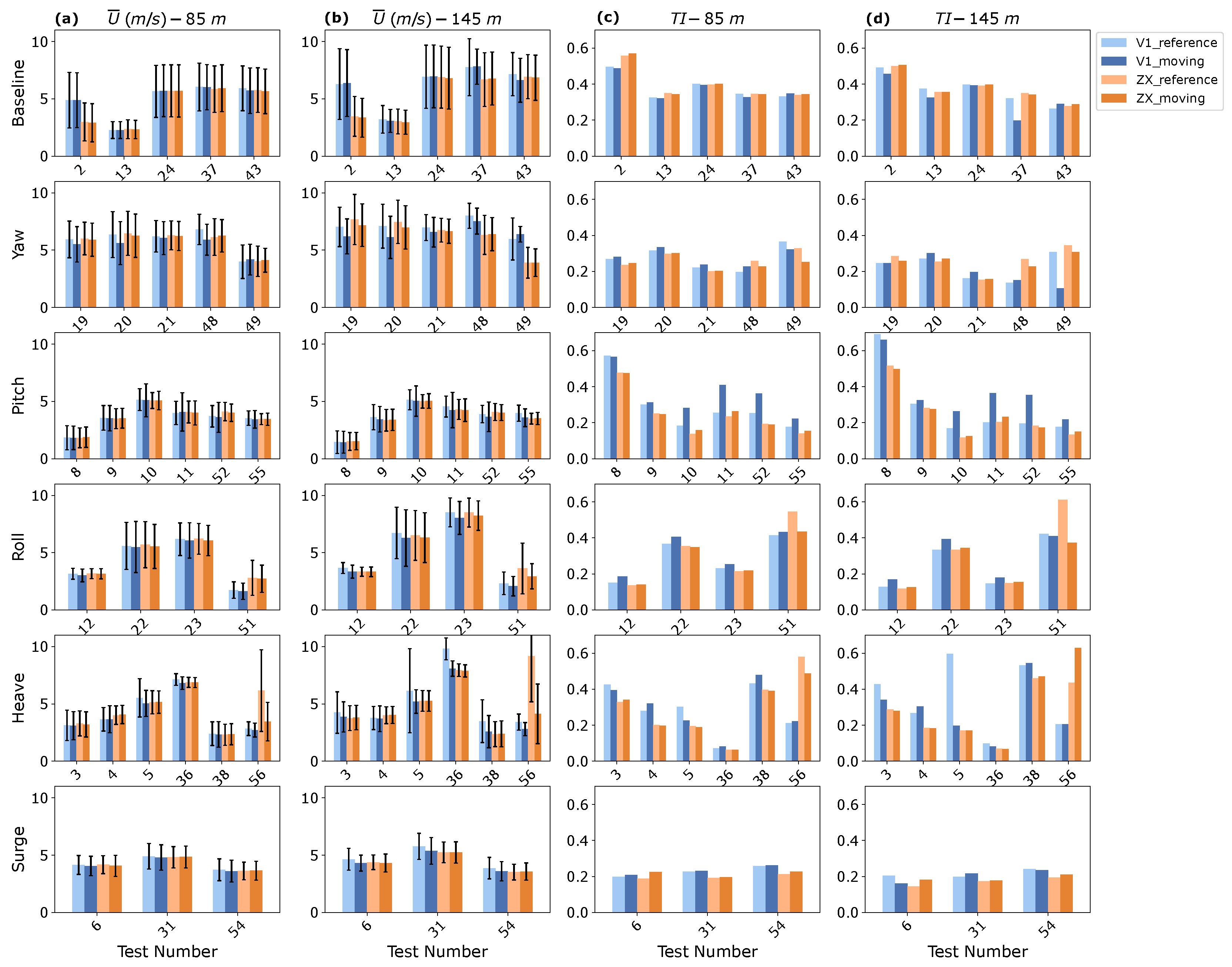
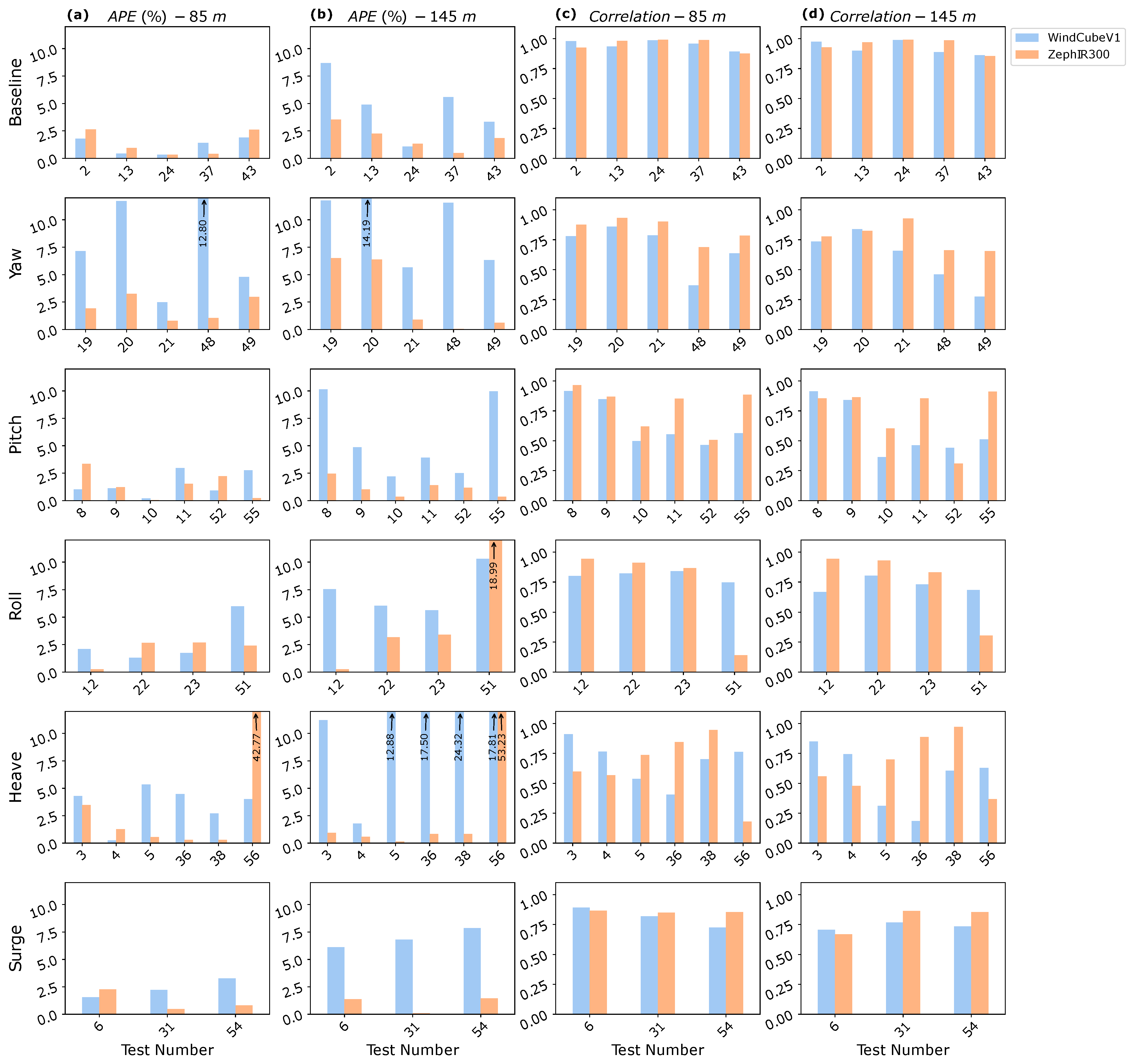
  • Yaw motion with a frequency close to the sampling frequency of the lidar can cause underestimation of mean wind speed for moving lidars. In our observations, the APE for the WindCube V1 exceeded 14%, while for the ZephIR 300 the APE remained below 6%.
    The correlation between the moving and reference lidars varied between 0.25 and 0.75, while the ZephIR 300 lidars showed a higher correlation than WindCube V1 at all yaw test cases.
  • Pitch motion (rotation along the N–S direction) with moderate frequency did not cause a significant discrepancy. Yet, as the motion amplitude increased, APE between the moving and reference lidar for both types increased following with a drop in correlation between lidars. This was the case for TI estimates as well. Our results showed that the motion-induced errors are affected more by pitch motion amplitude than by motion frequency.
  • Roll motion (rotation along the E–W direction) showed a marginally lower average wind speed for moving lidars compared to the reference lidars at both 85 m and 145 m. Additionally, their TI estimations were higher than reference lidars at both heights. Higher TI was observed in higher frequency test cases. The APE between moving and reference lidars was observed to be less than 5%. The high correlation between lidars persisted even with motion, but a decline in correlation was observed at the greater height (145 m).
  • Heave motion (vertical motion along the Z-axis) caused the moving lidars to measure mean wind speeds equal to or slightly lower than reference lidars. The WindCube V1 lidars had a higher discrepancy in TI estimations than ZephIR 300. The APE between the moving and reference lidars was less than 5% for both types at 85 m while this value increased for WindCube at 145 m.
  • Surge motion (horizontal movement in N–S direction) results showed the moving and reference lidars had similar mean wind speeds and APE less than 2.5% in 85 m and less than 7.5% at 145 m. In these test cases, strong correlation between lidars was observed. TI estimates of moving lidars were higher than those of the reference lidars. Our results showed that while surge motion had negligible effect on the ZephIR 300, the WindCube V1 had susceptibility to motion-induced errors.
Ultimately, the WindCube V1 showed larger variations before and after motion compensation compared to the ZephIR 300. However, the applied motion compensation was effective for both lidars, and the motion-induced errors were reduced by 85% and 82% after motion compensation, respectively.

Author Contributions

Conceptualization, J.R., J.G. and F.K.; methodology, C.D., F.K., A.D.J. and S.M.; validation, S.M. and C.D.; formal analysis, S.M.; data curation, S.M., F.K., C.D. and A.D.J.; writing—original draft preparation, S.M.; writing—review and editing, C.D., F.K., A.D.J., J.G. and J.R.; visualization, S.M.; supervision, F.K., J.G. and J.R.; funding acquisition, J.R. All authors have read and agreed to the published version of the manuscript.

Funding

This work was funded by the European Union Horizon 2020 research and innovation program under grant agreement no. 861291 as part of the Train2Wind Marie Sklodowska-Curie Innovation Training Network (https://www.train2wind.eu/, accessed on 27 August 2023). The Grimstad motion experiment in 2011 was performed as part of the project “Autonome målinger av vindprofil, strømprofil og bølger for kartlegging av nergipotensialet, design og operasjon av vindmøller til havs” funded by the Research council of Norway (RCN) under grant number 200646; the lidar instrumentation was provided by the National Norwegian infrastructure projects EFOWI (grant number: 197804) and OBLO (grant number: 227777), also funded by RCN. The six-degree-of-freedom motion platform, operated by the University of Agder, was provided by the FME NORCOWE (RCN grant number: 193821).

Data Availability Statement

The raw data supporting the conclusions of this article will be made available by the authors on request.

Acknowledgments

The authors are grateful to Jon Oddvar Hellevang, Stian Husevik Stavland, and Ivar Øyvind Sand, from former Christian Michelsen Research (CMR), now Norwegian Research Centre (NORCE), as well as Martin Flügge from GFI/UiB, now Andøya Space, for the preparation and realization of the experimental setup and the lidar operations during the Grimstad experiment. Great thanks to Eivind Arne Johansen and Geir Hovland from the University of Agder for helping out with the practicalities of setting up this test and for the operation of the six-DOF motion platform. Special thanks to Etienne Cheynet and Mauro Ghirardelli for their invaluable contributions in reviewing the manuscript, providing feedback, and engaging in insightful discussions.

Conflicts of Interest

The authors declare no conflicts of interest.

Abbreviations

The following abbreviations are used in this manuscript:
APEAbsolute Percentage Error
CNRCarrier-to-Noise Ratio
CWContinuous Wave
DBSDoppler Beam Swinging
DOFDegree of Freedom
FLSFloating Lidar System
LOSLine of Sight
MADMean Absolute Deviation
NaNNot a Number
TITurbulence Intensity
UTCUniversal Time Coordinated
VADVelocity Azimuth Display

Appendix A. Test Specifications

Table A1. Description of the motion patterns applied during the different tests.
Test No.Start TimeMotionAmplitude ( A 0 )Frequency ( f 0 )Comments
012011-08-16 15:50initial testvariable motions
022011-08-16 17:43baselineno movement--
032011-08-17 06:33heave40 cm0.1 Hz-
042011-08-17 10:04heave40 cm0.2 Hz-
052011-08-17 13:33heave40 cm0.15 Hz-
062011-08-17 16:52surge (N–S)40 cm0.1 Hz-
072011-08-17 20:22baselineno movement-WLS7-65 not measuring; condensation on the lens
082011-08-18 06:28tilt (N–S)0.2 Hz-
092011-08-18 08:52tilt (N–S)0.2 Hz-
102011-08-18 11:32tilt (N–S)10°0.2 Hz-
112011-08-18 14:34tilt (N–S)15°0.2 Hz-
122011-08-18 18:01tilt (E–W)15°0.2 Hz-
132011-08-18 20:21baselineno movement--
142011-08-19 06:26circle (N–S)30 cm0.2 Hz-
152011-08-19 09:32circle & tilt (N–S)30 cm & 5°0.2 Hz-
162011-08-19 12:42circle & tilt (N–S)30 cm & 10°0.2 Hz-
172011-08-19 16:22circle & tilt (N–S)30 cm & 3°0.2 Hz-
182011-08-19 19:52baselineno movement-WLS7-65 not measuring; condensation on the lens
192011-08-20 06:13yaw39°0.1 Hz-
202011-08-20 09:32yaw39°0.2 Hz-
212011-08-20 12:42yaw39°0.05 Hz-
222011-08-20 15:02tilt (E–W)10°0.2 Hz-
232011-08-20 17:44tilt (E–W)0.2 Hz-
242011-08-20 20:32baselineno movement--
252011-08-21 05:21tilt (E–W)0.2 Hz-
262011-08-21 10:05tilt (E–W)0.1 Hz-
272011-08-21 12:55tilt (E–W)0.1 Hz-
282011-08-21 15:31tilt (E–W)10°0.1 Hz-
292011-08-21 17:33tilt (E–W)15°0.1 Hz-
302011-08-21 21:01baselineno movement-WLS7-65 not measuring; condensation on the lens
312011-08-22 06:42surge (N–S)40cm0.1 Hz-
322011-08-22 09:04circle & tilt (N–S)30 cm & 12.5°0.1 Hz-
332011-08-22 12:01circle & tilt (N–S)30 cm & 12.5°0.2 Hz-
342011-08-22 14:32circle & tilt (N–S)30 cm & 5°0.1 Hz-
352011-08-22 16:51circle & tilt (N–S)30 cm & 3°0.2 Hz-
362011-08-22 18:51heave40 cm0.1 Hz-
372011-08-22 19:41baselineno movement--
382011-08-23 06:22heave & tilt (N–S)40 cm & 5°0.1 Hz-
392011-08-23 10:35circle & tilt (N–S)30 cm & 3° + 3° offset0.2 Hz-
402011-08-23 13:01circle & tilt (N–S)30 cm & 5° + 5° offset0.2 Hz-
412011-08-23 15:34file: Fresh breezemax. 14°--
422011-08-23 18:01file: Stormmax. 21°--
432011-08-23 20:32baselineno movement--
442011-08-24 06:02file: HurricaneMax 21°--
452011-08-24 09:02file: Moderate breezeMax 14°--
462011-08-24 12:02file: Moderate galeMax 17°--
472011-08-24 15:22file: Strong galeMax 20°--
482011-08-24 17:11yaw39°0.15 Hz-
492011-08-24 18:44yaw39°0.025 Hz-
502011-08-24 20:12baselineNo movement--
512011-08-25 06:05tilt (E–W)15°0.1 Hz-
522011-08-25 08:31tilt (N–S)20°0.1 Hz-
532011-08-25 10:51circle & tilt (N–S)30 cm & 5°+5° offset0.2 Hz-
542011-08-25 12:31surge40 cm0.2 Hz-
552011-08-25 14:41tilt N–S10°0.1 Hz-
562011-08-25 16:12heave20 cm0.4 Hz-
572011-08-25 17:50stop---

Appendix B. Height Settings

Table A2. Height settings, test 1–test 10 (from the surface).
Moving LidarsReference Lidars
Level No.WindCube V1 (m)ZephIR 300 (m)WindCube V1 (m)ZephIR 300 (m)
10197197200200
9157157160160
8142142145145
7127127130130
6112112115115
59797100100
482828585
367677070
252525555
140404343
Table A3. Height settings, test 11–test 54 (from the surface).
Moving LidarsReference Lidars
Level No.WindCube V1 (m)ZephIR 300 (m)WindCube V1 (m)ZephIR 300 (m)
10197142200145
91578216085
81428214585
71278213085
61128211585
5978210085
482828585
367827085
252825585
140404343

References

  1. Veers, P.; Dykes, K.; Basu, S.; Bianchini, A.; Clifton, A.; Green, P.; Holttinen, H.; Kitzing, L.; Kosovic, B.; Lundquist, J.K.; et al. Grand Challenges: Wind energy research needs for a global energy transition. Wind. Energy Sci. Discuss. 2022, 2022, 1–8. [Google Scholar] [CrossRef]
  2. Fischer, G. Installation and Operation of the Research Platform FINO 1 in the North Sea. In Offshore Wind Energy; Köller, J., Köpper, J., Peters, W., Eds.; Springer: Berlin/Heidelberg, Germany, 2006; pp. 237–253. [Google Scholar] [CrossRef]
  3. Poveda Maureira, J.P.; Wouters, D.A.J. Wind Measurements at Meteorological Mast IJmuiden; Technical Report February; Report ECN-E–14-058; Energy Center of the Netherlands (ECN): Petten, The Netherlands, 2015. [Google Scholar]
  4. Hasager, C.B.; Peña, A.; Christiansen, M.B.; Astrup, P.; Nielsen, M.; Monaldo, F.; Thompson, D.; Nielsen, P. Remote sensing observation used in offshore wind energy. IEEE J. Sel. Top. Appl. Earth Obs. Remote Sens. 2008, 1, 67–79. [Google Scholar] [CrossRef]
  5. Liu, Z.; Barlow, J.F.; Chan, P.W.; Fung, J.C.H.; Li, Y.; Ren, C.; Mak, H.W.L.; Ng, E. A Review of Progress and Applications of Pulsed Doppler Wind LiDARs. Remote Sens. 2019, 11, 2522. [Google Scholar] [CrossRef]
  6. Reuder, J.; Cheynet, E.; Clifton, A.; van Dooren, M.F.; Gottschall, J.; Jakobsen, J.B.; Mann, J.; Palma, J.; Schlipf, D.; Sjøholm, M.; et al. Recommendation on Use of Wind Lidars; Technical report; Geophysical Institute and Bergen Offshore Wind Centre (BOW), University of Bergen: Bergen, Norway, 2021. [Google Scholar] [CrossRef]
  7. Gottschall, J.; Wolken-Möhlmann, G.; Lange, B. About offshore resource assessment with floating lidars with special respect to turbulence and extreme events. J. Phys. Conf. Ser. 2014, 555, 012043. [Google Scholar] [CrossRef]
  8. Wagner, R.; Pedersen, T.F.; Courtney, M.; Antoniou, I.; Davoust, S.; Rivera, R. Power curve measurement with a nacelle mounted lidar. Wind Energy 2014, 17, 1441–1453. [Google Scholar] [CrossRef]
  9. Bossanyi, E.; Kumar, A.; Hugues-Salas, O. Wind turbine control applications of turbine-mounted LIDAR. J. Phys. Conf. Ser. 2014, 555, 012011. [Google Scholar] [CrossRef]
  10. Gräfe, M.; Pettas, V.; Gottschall, J.; Cheng, P.W. Quantification and correction of motion influence for nacelle-based lidar systems on floating wind turbines. Wind Energy Sci. 2023, 8, 925–946. [Google Scholar] [CrossRef]
  11. Cañadillas, B.; Westerhellweg, A.; Neumann, T. Testing the Performance of a Ground-based Wind LiDAR System One Year Intercomparison at the Offshore. DEWI Mag. 2011, 38, 58–65. [Google Scholar]
  12. Hasager, C.B.; Stein, D.; Courtney, M.; Peña, A.; Mikkelsen, T.; Stickland, M.; Oldroyd, A. Hub height ocean winds over the north sea observed by the NORSEWInD lidar array: Measuring techniques, quality control and data management. Remote Sens. 2013, 5, 4280–4303. [Google Scholar] [CrossRef]
  13. Peña, A.; Gryning, S.E.; Floors, R. Lidar observations of marine boundary-layer winds and heights: A preliminary study. Meteorol. Z. 2015, 24, 581–589. [Google Scholar] [CrossRef]
  14. Gottschall, J.; Wolken-Möhlmann, G.; Viergutz, T.; Lange, B. Results and conclusions of a floating-lidar offshore test. Energy Procedia 2014, 53, 156–161. [Google Scholar] [CrossRef]
  15. Achtert, P.; Brooks, I.M.; Brooks, B.J.; Moat, B.I.; Prytherch, J.; Persson, P.O.G.; Tjernström, M. Measurement of wind profiles by motion-stabilised ship-borne Doppler lidar. Atmos. Meas. Tech. 2015, 8, 4993–5007. [Google Scholar] [CrossRef]
  16. Gottschall, J.; Catalano, E.; Dörenkämper, M.; Witha, B. The NEWA Ferry Lidar Experiment: Measuring Mesoscale Winds in the Southern Baltic Sea. Remote Sens. 2018, 10, 1620. [Google Scholar] [CrossRef]
  17. Duscha, C.; Paskyabi, M.B.; Reuder, J. Statistic and coherence response of ship-based lidar observations to motion compensation. J. Phys. Conf. Ser. 2020, 1669, 012020. [Google Scholar] [CrossRef]
  18. Kelberlau, F.; Neshaug, V.; Lønseth, L.; Bracchi, T.; Mann, J. Taking the Motion out of Floating Lidar: Turbulence Intensity Estimates with a Continuous-Wave Wind Lidar. Remote Sens. 2020, 12, 898. [Google Scholar] [CrossRef]
  19. Pichugina, Y.L.; Banta, R.M.; Brewer, W.A.; Sandberg, S.P.; Hardesty, R.M. Doppler Lidar–Based Wind-Profile Measurement System for Offshore Wind-Energy and Other Marine Boundary Layer Applications. J. Appl. Meteorol. Climatol. 2012, 51, 327–349. [Google Scholar] [CrossRef]
  20. Wolken-Möhlmann, G.; Gottschall, J.; Lange, B. First Verification Test and Wake Measurement Results Using a SHIP-LIDAR System. Energy Procedia 2014, 53, 146–155. [Google Scholar] [CrossRef]
  21. Duscha, C.; Barrell, C.; Renfrew, I.A.; Brooks, I.M.; Sodemann, H.; Reuder, J. A Ship-Based Characterization of Coherent Boundary-Layer Structures Over the Lifecycle of a Marine Cold-Air Outbreak. Bound.-Layer Meteorol. 2022, 183, 355–380. [Google Scholar] [CrossRef]
  22. Rubio, H.; Kühn, M.; Gottschall, J. Evaluation of low-level jets in the southern Baltic Sea: A comparison between ship-based lidar observational data and numerical models. Wind Energy Sci. 2022, 7, 2433–2455. [Google Scholar] [CrossRef]
  23. Hill, R.J.; Brewer, W.A.; Tucker, S.C. Platform-motion correction of velocity measured by Doppler lidar. J. Atmos. Ocean. Technol. 2008, 25, 1369–1382. [Google Scholar] [CrossRef]
  24. Gottschall, J.; Gribben, B.; Stein, D.; Würth, I. Floating lidar as an advanced offshore wind speed measurement technique: Current technology status and gap analysis in regard to full maturity. Wiley Interdiscip. Rev. Energy Environ. 2017, 6, e250. [Google Scholar] [CrossRef]
  25. Désert, T.; Knapp, G.; Aubrun, S. Quantification and Correction of Wave-Induced Turbulence Intensity Bias for a Floating LIDAR System. Remote Sens. 2021, 13, 2973. [Google Scholar] [CrossRef]
  26. Gutiérrez-Antuñano, M.; Tiana-Alsina, J.; Salcedo, A.; Rocadenbosch, F. Estimation of the Motion-Induced Horizontal-Wind-Speed Standard Deviation in an Offshore Doppler Lidar. Remote Sens. 2018, 10, 2037. [Google Scholar] [CrossRef]
  27. Kelberlau, F.; Mann, J. Quantification of motion-induced measurement error on floating lidar systems. Atmos. Meas. Tech. 2022, 15, 5323–5341. [Google Scholar] [CrossRef]
  28. Tucker, S.C.; Senff, C.J.; Weickmann, A.M.; Brewer, W.A.; Banta, R.M.; Sandberg, S.P.; Law, D.C.; Hardesty, R.M. Doppler Lidar Estimation of Mixing Height Using Turbulence, Shear, and Aerosol Profiles. J. Atmos. Ocean. Technol. 2009, 26, 673–688. [Google Scholar] [CrossRef]
  29. Zentek, R.; Kohnemann, S.H.E.; Heinemann, G. Analysis of the performance of a ship-borne scanning wind lidar in the Arctic and Antarctic. Atmos. Meas. Tech. 2018, 11, 5781–5795. [Google Scholar] [CrossRef]
  30. Bischoff, O.; Schlipf, D.; Würth, I.; Cheng, P. Dynamic Motion Effects and Compensation Methods of a Floating Lidar Buoy. In Proceedings of the EERA DeepWind 2015 Deep Sea Offshore Wind Conference, Trondheim, Norway, 4–6 February 2015; pp. 4–6. [Google Scholar]
  31. Thebault, N.; Thiébaut, M.; Le Boulluec, M.; Damblans, G.; Maisondieu, C.; Benzo, C.; Guinot, F. Experimental evaluation of the motion-induced effects on turbulent fluctuations measurement on floating lidar systems. Wind Energy Sci. Discuss. 2023, 2023, 1–22. [Google Scholar]
  32. Banakh, V.A.; Smalikho, I.N.; Köpp, F.; Werner, C. Representativeness of wind measurements with a CW Doppler lidar in the atmospheric boundary layer. Appl. Opt. 1995, 34, 2055–2067. [Google Scholar] [CrossRef] [PubMed]
  33. Peña, A.; Hasager, C.B.; Lange, J.; Anger, J.; Badger, M.; Bingöl, F.; Bischoff, O.; Cariou, J.P.; Dunne, F.; Emeis, S.; et al. Remote Sensing for Wind Energy; DTU Wind Energy: Roskilde, Denmark, 2013. [Google Scholar]
  34. Haakenstad, H.; Breivik, Ø.; Furevik, B.R.; Reistad, M.; Bohlinger, P.; Aarnes, O.J. NORA3: A nonhydrostatic high-resolution hindcast of the North Sea, the Norwegian Sea, and the Barents Sea. J. Appl. Meteorol. Climatol. 2021, 60, 1443–1464. [Google Scholar] [CrossRef]
  35. Pearson, G.; Davies, F.; Collier, C. An analysis of the performance of the UFAM pulsed Doppler lidar for observing the boundary layer. J. Atmos. Ocean. Technol. 2009, 26, 240–250. [Google Scholar] [CrossRef]
  36. Pham-Gia, T.; Hung, T.L. The mean and median absolute deviations. Math. Comput. Model. 2001, 34, 921–936. [Google Scholar] [CrossRef]
  37. Leys, C.; Ley, C.; Klein, O.; Bernard, P.; Licata, L. Detecting outliers: Do not use standard deviation around the mean, use absolute deviation around the median. J. Exp. Soc. Psychol. 2013, 49, 764–766. [Google Scholar] [CrossRef]
  38. Duscha, C. Characterizing the Convective Boundary Layer with Wind-Profiling and Scanning Doppler Lidar. Ph.D. Thesis, The University of Bergen, Bergen, Norway, 2024. [Google Scholar]
Figure 1. Lidars on the moving platform. A WindCube V1 and a ZephIR 300 were mounted on a moving Hexapod; reference lidars were placed 5 m west of the moving ones.
Remotesensing 16 03191 g001
Figure 2. Grimstad experiment location. This experiment took place at the campus of University of Adger South-West of Norway.
Remotesensing 16 03191 g002
Figure 3. Coordinate system and angles for lidars. The laser beam is emitted at a fixed elevation angle ( ϕ ) and at an azimuth angle ( α ). The half–opening angle ( θ ) equals 90 ° ϕ . The LOS velocity ( v r ) at height h is linked to the three-dimensional wind velocity vector and the corresponding angles.
Remotesensing 16 03191 g003
Figure 4. Impact of (a) rotational, (b) translational, and (c) combined motion on the observed LOS velocity ( v r , o ) and the retrieved velocity ( u ^ ) in the Cartesian reference frame.
Remotesensing 16 03191 g004
Figure 5. Comparison of wind speed on 2011-08-17 for the reference lidar before and after applying the MAD filter. Raw data are shown in gray and the filtered data are shown in orange. The median is shown as a dark-red dashed line, and the dotted gray lines represent the thresholds.
Remotesensing 16 03191 g005
Figure 6. Mean horizontal wind speed measured by WindCube V1 (blue) and ZephIR 300 (orange) at 85 m (a) and 145 m (b). Turbulence intensity estimate at 85 m (c) and 145 m (d). The bars with darker shades represent the measurements from the reference lidar and the bars with lighter shades represent the measurements by moving lidars. Error bars also represent the standard deviations. The width of the bars does not convey any specific information. Each panel shows one type of motion.
Remotesensing 16 03191 g006
Figure 7. Absolute percentage error (APE) between moving and reference lidars (WindCube V1 in blue and ZephIR 300 in orange) at 85 m (a) and 145 m (b). Additionally, correlations between moving and reference lidars are shown at 85 m (c) and at 145 m (d). The width of the bars does not convey any specific information.
Remotesensing 16 03191 g007
Figure 8. Top view of one VAD scan for WindCube V1 and the beam’s corresponding azimuth angle. α shows the position of beam when there is no motion (gray) and α shows the beam position when exposed to yaw motion with a frequency similar to beam swinging frequency (red).
Remotesensing 16 03191 g008
Figure 9. Comparison of wind speed time series before and after motion correction in a 15 min time slice for test 11. (a) WindCube V1 reference (purple) vs. WindCube V1 moving before compensation (light green), (b) ZephIR 300 reference (orange) vs. ZephIR 300 moving before compensation (light blue), (c) WindCube V1 reference (purple) vs. WindCube V1 moving after compensation (dark green), and (d) ZephIR 300 reference (orange) vs. ZephIR 300 moving after compensation (dark blue) (Courtesy of Christiane Duscha [38]).
Remotesensing 16 03191 g009
Figure 10. Distribution of the error between WindCube V1 moving and WindCube V1 reference before compensation (a) and after compensation (c). Distribution of error between ZephIR 300 moving and reference before compensation (b) and after compensation (d).
Remotesensing 16 03191 g010
Figure 11. Wind speed scatter plot before and after motion correction for test 11. (a) WindCube V1 reference (x) vs. WindCube V1 moving before compensation (y), (b) ZephIR 300 reference (x) vs. ZephIR 300 moving before compensation (y), (c) WindCube V1 reference (x) vs. WindCube V1 moving after compensation (y), and (d) ZephIR 300 reference (x) vs. ZephIR 300 moving after compensation (y) (Courtesy of Christiane Duscha [38]). The red line represents the Deming regression.
Remotesensing 16 03191 g011
Disclaimer/Publisher’s Note: The statements, opinions and data contained in all publications are solely those of the individual author(s) and contributor(s) and not of MDPI and/or the editor(s). MDPI and/or the editor(s) disclaim responsibility for any injury to people or property resulting from any ideas, methods, instructions or products referred to in the content.

