Spatiotemporal Distribution, Sources, and Impact on Atmospheric Oxidation of Reactive Nitrogen Oxides in the North China Plain Agricultural Regions in Summer

Abstract

The lack of vertical observation of reactive nitrogen oxides in agricultural areas has posed a significant challenge in fully understanding their sources and impacts on atmospheric oxidation. Ground-based multi-axis differential optical absorption spectroscopy (MAX-DOAS) observations were conducted in the agricultural regions of the North China Plain (NCP) during the summer of 2019 to measure the vertical distributions of aerosols, nitrogen dioxide (NO₂), and nitrous acid (HONO). This study aimed at revealing the spatiotemporal distribution, sources, and environmental effects of reactive nitrogen oxides in the NCP agricultural areas. Our findings indicated that the vertical profiles of aerosols and NO₂ exhibited a near-Gaussian distribution, with distinct peak times occurring between 8:00–10:00 and 16:00–18:00. HONO reached its maximum concentration near the surface around 8:00 in the morning and decreased exponentially with altitude. After sunrise, the concentration of HONO rapidly decreased due to photolysis. Additionally, the potential source contribution function (PSCF) was used to evaluate the potential sources of air pollutants. The results indicated that the main potential pollution sources of aerosols were located in the southern part of the Hebei, Shanxi, Shandong, and Jiangsu provinces, while the potential pollution sources of NO₂ were concentrated in the Beijing–Tianjin–Hebei region. At altitudes exceeding 500 m, the heterogeneous reactions of NO₂ on aerosol surfaces were identified as one of the important contributors to the formation of HONO. Furthermore, we discussed the production rate of hydroxyl radicals (OH) from HONO photolysis. It was found that the production rate of OH from HONO photolysis decreased with altitude, with peaks occurring in the morning and late afternoon. This pattern was consistent with the variations in HONO concentration, indicating that HONO was the main contributor to OH production in the agricultural regions of the NCP. This study provides a new perspective on the sources of active nitrogen in agricultural regions and their contribution to atmospheric oxidation capacity from a vertical perspective.

1. Introduction

Nitrous acid (HONO) plays a critical role in the atmospheric nitrogen cycle by producing hydroxyl radical (OH) through photolysis, thereby influencing atmospheric oxidation capacity [1,2,3,4]. Up to 20–90% of OH formation has been attributed to HONO photolysis [5,6,7,8]. Primary pollutants in the atmosphere, such as carbon monoxide (CO), nitrogen oxides (NO_x), and volatile organic compounds (VOCs), can be oxidized by OH, promoting the formation of ozone (O₃) and secondary aerosols [9,10]. High concentrations of HONO may seriously threaten people’s health because long-term exposure may harm lung function [11,12]. Additionally, the reaction between HONO and ammonia (NH₃) can produce carcinogenic nitrosamines [13]. Despite extensive research on HONO over the years, there is still no consensus on its sources. A substantial amount of research indicates that the sources of HONO can be classified into four categories [14]: (1) homogeneous reactions between nitric oxide (NO) and OH (R1) [15,16,17], (2) direct emissions from vehicle exhaust, soil, and biomass combustion [18,19,20], (3) heterogeneous reactions of nitrogen dioxide (NO₂) on wet surfaces (R2) [16,21], and (4) photolysis of nitrate particles in the soil and atmosphere (R3) [15,22]. Reaction (R1) almost exclusively occurs during daytime, under conditions of high NO and OH concentrations [23]. Reaction (R2), particularly on aerosol surfaces, is an important source of HONO and the main source of nighttime HONO [5]. Furthermore, the surface area density and chemical nature of aerosols are the dominant factors controlling the conversion efficiency of NO₂ to HONO [24]. Reaction (R3) is closely associated with agricultural activities.

$$NO+OH+M\to HONO+M$$

(R1)

$$2N{O}_2+H_{2}O+surface\to HONO+HN{O}_3$$

(R2)

$$HN{O}_3/N{O}_3^{-}+hv\to HONO/N{O}_2^{-}+O$$

(R3)

In agricultural areas, the extensive use of nitrogen fertilizers has become a significant source of soil emissions of HONO, impacting air quality [25]. Therefore, it is essential to understand the sources, spatiotemporal distribution, and environmental effects of HONO in agricultural regions. In the agricultural regions of Wangdu in the NCP, it has been found that soil fertilization is an important source of HONO [26]. Observations conducted in the agricultural areas of the Huai River Basin revealed that the heterogeneous reactions involving surface NO₂ serve as the primary contributor to the formation of nighttime HONO [25]. Moreover, after fertilization, farms released large amounts of HONO, leading to increased HONO concentrations and a higher HONO-to-NO₂ ratio [27]. However, these studies mentioned above primarily focused on near-surface observations, lacking insight into the sources and environmental effects of HONO at different altitudes in agricultural regions. Research in urban areas has shown that during haze events, high-altitude HONO mainly originates from heterogeneous reactions of NO₂ on aerosol surfaces rather than near-surface diffusion [28]. Therefore, by detecting the vertical distribution of HONO, we can obtain a better understanding of its sources and contribution to atmospheric oxidation capacity [29].

Currently, common vertical observation methods for HONO include tower observations [28,30,31], airborne and balloon-borne observations [32,33,34], long-path differential optical absorption spectroscopy (LP-DOAS) observations [35,36], and multi-axis differential optical absorption spectroscopy (MAX-DOAS) remote sensing observations [1,5,37]. However, tower observations can only measure the concentrations of atmospheric pollutants up to 400 m [38]. Observations conducted via airborne and balloon platforms face constraints related to flight time, posing difficulties for prolonged continuous monitoring [39]. Although the LP-DOAS technique facilitates non-contact and continuous measurements, its operational altitude remains restricted. As a promising spectral remote sensing technology, MAX-DOAS can obtain real-time and continuous vertical distributions of atmospheric pollutants [40,41,42,43]. In recent years, MAX-DOAS has been used worldwide for HONO observations, including in Madrid, Spain [1], Melbourne, Australia [37], Beijing, China [5], and Leshan, China [44].

Even though MAX-DOAS has been used to observe HONO in several locations in China, most observation sites are in urban regions, and few studies have focused on agricultural sources. Therefore, in this study, MAX-DOAS observation experiments were carried out in the agricultural regions of the NCP to investigate the spatiotemporal distributions and potential sources of aerosols, NO₂, and HONO. In addition, considering the critical role of aerosols in the heterogeneous reaction of NO₂ to HONO, we analyzed the relationship between aerosols and the conversion rate from NO₂ to HONO. Furthermore, based on vertical observations of HONO, this study opens a new window on rethinking the sources of reactive nitrogen oxides in agricultural regions and their contribution to atmospheric oxidation capacity from a vertical perspective.

The structure of this work is outlined as follows: Section 2 details the MAX-DOAS observation campaign, the retrieval algorithm for pollutants, the Potential Source Contribution Function (PSCF), and additional supporting data. In Section 3, the potential sources and spatiotemporal distribution of pollutants are presented. The formation of HONO through the heterogeneous reactions of NO₂, and OH radicals from HONO photolysis are evaluated. In Section 4, further analyses of the results are conducted, along with comparisons to results from other regions.

2. Materials and Methods

2.1. MAX-DOAS Measurement Setup

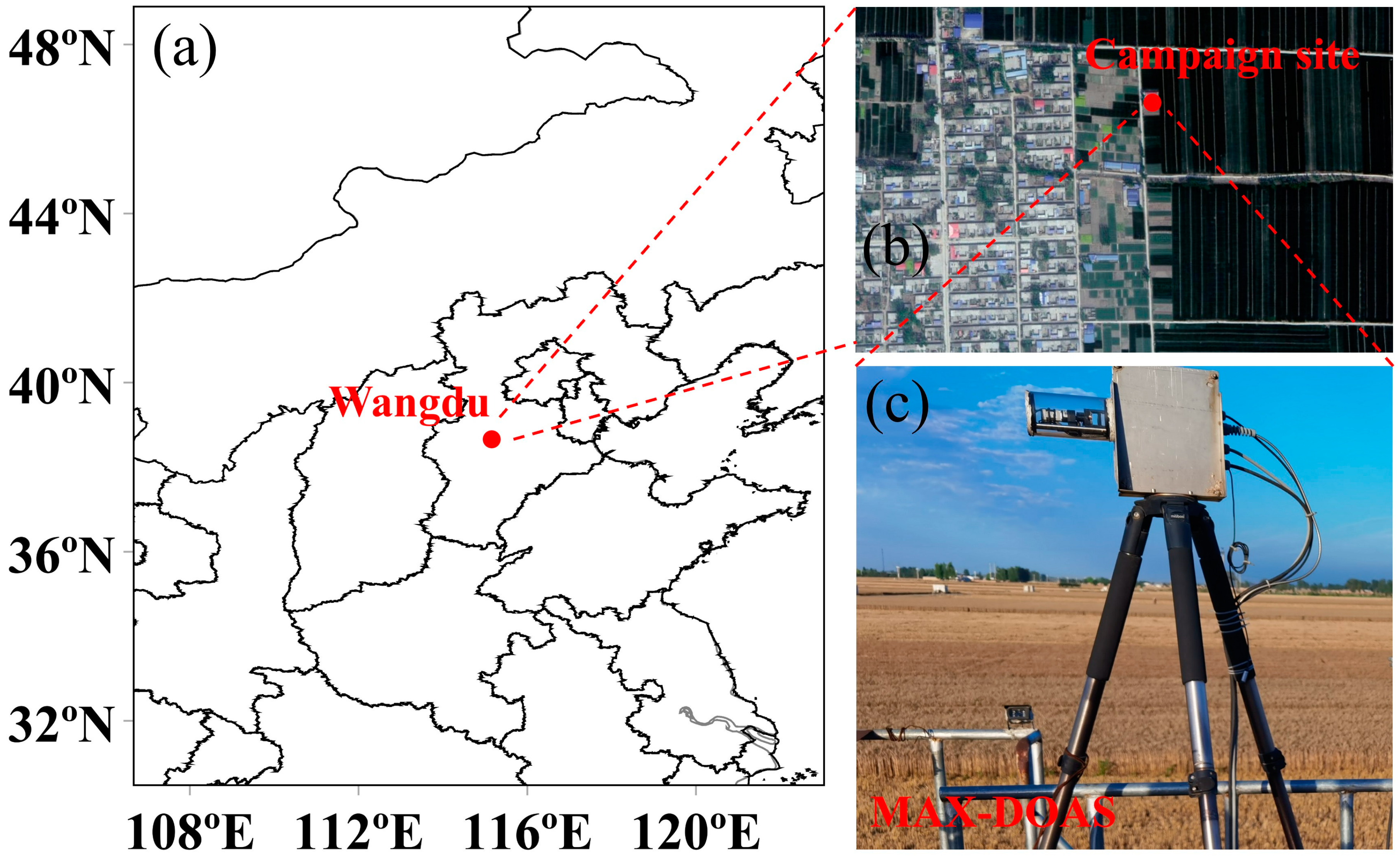
The MAX-DOAS instrument was set up at the Rural Environmental Research Station of the Research Center for Eco-Environmental Sciences, Chinese Academy of Sciences (115.26°E, 38.68°N), located in Wangdu County, Baoding City, in the NCP, from 1 June 2019 to 31 August 2019 (Figure 1). The Wangdu station is surrounded by farmland where winter wheat and summer maize are grown in rotation, with almost no industrial emission sources nearby [27,45]. This setup aimed to study the vertical distributions, potential sources, and contribution to atmospheric oxidation of reactive nitrogen oxides in agricultural environments. The station is situated at an altitude of 35 m, and the observational azimuth angle was set to 78°. The instrument consists of a telescope system and a spectral analysis system. In the telescope system, a quartz right-angle prism, rotated by a stepper motor, receives scattered sunlight at different elevation angles. After passing through the prism, the sunlight gathers through a plano-convex lens to the optical fiber entrance, and eventually enters the spectral analysis system. The field of view (FOV) of the telescope system is less than 0.5°, and the elevation accuracy is better than 0.1°. The spectral analysis system primarily consists of two Avantes spectrometers, which split the collected scattered sunlight and convert the light signal into an electrical signal using a Charge-Coupled Device (CCD), thus obtaining spectral data from the scattered light. Because the CCD is highly sensitive to temperature changes, its temperature is maintained at 20 ± 0.5 °C by a temperature sensor and a semiconductor cooling device near the CCD. The effective spectral range collected by the instrument is 300–500 nm, with a spectral resolution of 0.49 nm. Further detailed descriptions of the instrument can be found in previous studies [46,47].

During the observation period, each observation series consisted of 11 elevation angles: 1, 2, 3, 4, 5, 6, 8, 10, 15, 30, and 90°. The integration time for each elevation angle was adjusted according to the solar zenith angle (SZA), with the single exposure time and scan number automatically adjusted based on the light intensity. It takes about 12 min to complete an observation series.

2.2. Spectral Analysis

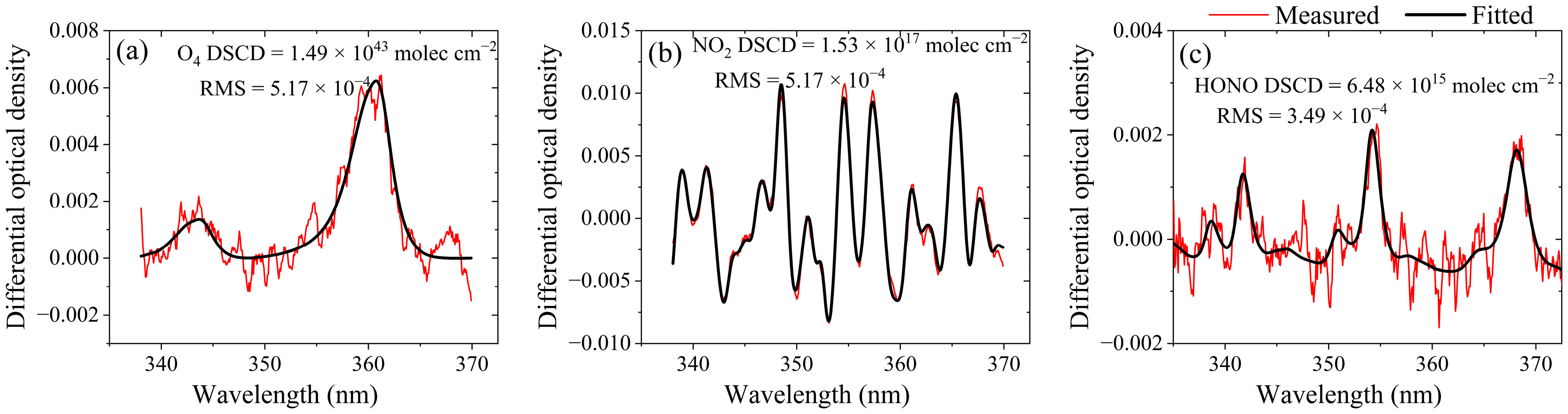
The differential slant column densities (DSCDs) of aerosols, NO₂, and HONO were retrieved using the QDOAS software (version 3.4) developed by the Belgian Institute for Space Aeronomy (BIRA-IASB) (http://uv-vis.aeronomie.be/software/QDOAS/, accessed on 22 March 2024). Before spectral analysis, dark current and electronic offset were subtracted from the spectra, and wavelength calibration was performed with a standard mercury lamp [48,49]. Additionally, cloud effects are filtered out based on color index [50,51,52,53], as detailed in Section S1.

Table 1. Summary of DOAS retrieval settings of O₄, NO₂, and HONO.

Parameter	Data Source	Trace Gases
		O4	NO2	HONO
Wavelength Range (nm)		338–370	338–370	335–373
NO2	220 K, 298 K, I0-corrected * [54]	√	√	√
O3	223 K, 243 K, I0-corrected * [55]	√	√	√
O4	293 K [56]	√	√	√
HCHO	298 K [57]	√	√	√
H2O	HITEMP [58]	✕	✕	√
BrO	223 K [59]	√	√	√
HONO	296 K [60]	✕	✕	√
Ring	Calculated with QDOAS	√	√	√
Polynomial degree		Order 5	Order 5	Order 5
Intensity offset		Constant	Constant	Constant
Wavelength calibration	Based on a high resolution solar reference spectrum (SAO2010 solar spectral) [61]

* Solar I₀-correction [62].

provides the detailed retrieval settings for O₄, H₂O, NO₂, and HONO. The details about the Ring effect and I₀ effect can be found in Section S2. An example of DOAS fitting results for a measured spectrum with an elevation of 4° and a solar zenith angle of 72.32° on 6 June 2019, is shown in Figure 2. To ensure the reliability of the DOAS retrieval, NO₂ and HONO DSCDs were excluded when the root mean square (RMS) of fitting residuals exceeded 2 × 10⁻³. As a result, the corresponding qualified DSCD results of NO₂ and HONO were 85.84% and 90.81%, respectively.

2.3. Vertical Profile Retrievals

In this study, the vertical profiles of aerosols, NO₂, and HONO were retrieved based on the Heidelberg Profile retrieval algorithm (HEIPRO) [63,64]. This algorithm relies on the Optimal Estimation Method (OEM) and utilizes the radiative transfer model SCIATRAN (version 2.2) as the forward model [65]. The so-called maximum a posteriori (MAP) solution is obtained from the following cost function:

$${\chi }^2\left(x\right)=\left[y-F\left(x,b\right){]}^T{S}_{\epsilon }^{-1}\right[y-F\left(x,b\right)\left]+\right[x-x_a{]}^T{S}_a^{-1}\left[x-x_a\right]$$

(1)

Here, $x$ is the aerosols or trace gas profiles; $y$ is the DSCDs of different components at different elevation angles; $F\left(x,b\right)$ is the forward model simulation value of DSCDs; $b$ is meteorological parameters (e.g., pressure and temperature vertical profiles); $x_a$ is prior information; $S_a$ is the covariance matrix of $x$; and $S_{\epsilon }$ is the covariance matrix of $y$. In the retrieved process, the optical parameters of the aerosols were selected as follows: the asymmetry parameter was 0.7, the surface albedo was 0.05, and the single scattering albedo was 0.95 [66]. The atmosphere was divided into 20 layers from 0 to 2 km, each with a thickness of 100 m. The time resolution of the vertical profiles was set to 15 min to ensure that a complete observation elevation series could be covered. The aerosol optical depth (AOD), which measures the extent to which aerosols prevent the transmission of sunlight by absorption or scattering, and the vertical column densities (VCD), which represent the total number of molecules of trace gases in a column of air extending from the ground to the top of the atmosphere, were obtained by integrating the concentrations at different heights. The detailed retrievals process can be found in Figure S1.

2.4. Calculation of Pollutant Growth Percentages during Haze Days Compared to Non-Haze Days

According to the China Meteorological Administration’s haze standard (QX/T 113-2010), weather conditions are classified into two categories based on visibility and relative humidity: non-haze days (visibility > 10 km) and haze days (visibility < 10 km and RH < 80%) [67,68,69]. Haze days accounted for 11% of the data, while non-haze days accounted for 89%.

Compared to non-haze days, the growth percentages of atmospheric pollutants on haze days can be expressed as follows:

$$G={\displaystyle \frac{{\left[P\right]}_{nonhaze}-{\left[P\right]}_{haze}}{{\left[P\right]}_{nonhaze}}}\times 100\%$$

(2)

Here, $G$ represents the growth percentages of atmospheric pollutants. The average concentrations of atmospheric pollutants at different altitudes on non-haze and haze days are, respectively, represented by ${\left[P\right]}_{nonhaze}$ and ${\left[P\right]}_{haze}$.

2.5. PSCF Analysis

The Hybrid Single-Particle Lagrangian Integrated Trajectory (HYSPLIT) model with the Global Data Assimilation System (GDAS) was developed by the National Oceanic and Atmospheric Administration Air Resource Laboratory to calculate the backward trajectories of air masses.

The Potential Source Contribution Function (PSCF) is an effective method for identifying pollution source distributions and transport paths based on pollutant concentrations and backward trajectories [70,71]. First, the study area is divided into several grids, and $N_{ij}$ is defined as the total number of trajectory endpoints within the $ij$th grid cell. Using the average aerosol extinction and NO₂ concentrations during the observation period as the threshold values, $M_{ij}$ is defined as the total number of endpoints with a pollutant concentration higher than the threshold within the $ij$th grid cell. The $PSCF$ within the $ij$th grid cell is defined as follows:

$$PSC{F}_{ij}={\displaystyle \frac{M_{ij}}{N_{ij}}}$$

(3)

Because PSCF is a conditional probability, considerable uncertainty occurs when the value of $N_{ij}$ is small. In order to reduce the influence of uncertainty, $W_{ij}$ was defined as the weight factor of the $ij$th grid cell, determined by $N_{ij}$. Therefore, the $PSC{F}_{ij}$ is multiplied by the $W_{ij}$, resulting in the weighted PSCF (WPSCF). The detailed settings of $W_{ij}$ are as follows:

$$W_{ij}=\left\{\begin{array}{c}1.0 N_{ij}>3N_{ave}\\ 0.7 3N_{ave}>N_{ij}>{\displaystyle \frac{3}{2}}{N}_{ave}\\ 0.4 {\displaystyle \frac{3}{2}}{N}_{ave}>N_{ij}>N_{ave}\\ 0.2 N_{ave}>N_{ij}\end{array}\right.$$

(4)

where $N_{ave}$ represents the average number of endpoints per grid. The $WPSCF$ within the $ij$th grid cell is defined as follows:

$$WPSC{F}_{ij}=W_{ij}\times PSC{F}_{ij}$$

(5)

In this study, the backward trajectories and WPSCF of the observation site were analyzed using TrajStat software (version 1.5.5) [72,73,74].

2.6. Calculation of Conversion Rate from NO₂ to HONO

The data showing an increase in the ratio of HONO to NO₂ over a continuous three-hour period were used to calculate the conversion rate from NO₂ to HONO [62,66]:

$$C\left(HONO\right)={\displaystyle \frac{\frac{{\left[HONO\right]}_{t_2}}{{\left[N{O}_2\right]}_{t_2}}-\frac{{\left[HONO\right]}_{t_1}}{{\left[N{O}_2\right]}_{t_1}}}{t_2-t_1}}$$

(6)

Here, $C\left(HONO\right)$ represents the conversion rate from NO₂ to HONO; $\left[HONO\right]$ and $\left[N{O}_2\right]$ represent the concentration of NO₂ and HONO, respectively; and $t_2$ and $t_1$ represent the initial and final times, respectively.

2.7. TUV Model and OH Generation Rate Calculation

The Tropospheric Ultraviolet–Visible Model (TUV) was used to calculate the photolysis frequency of HONO [75]. The total ozone column input into the model was obtained from TROPOMI observation, the AOD at 360.8 nm was obtained from the MAX-DOAS instrument, and the single scattering albedo (SSA) was 0.95 [76]. The TUV model has been widely used in observations based on the MAX-DOAS instrument [5,37,77].

The contribution of HONO to the OH generation rate ($P{\left(OH\right)}_{HONO}$) can be calculated using the following formula [44,66]:

$$P{\left(OH\right)}_{HONO}=J\left(HONO\right)\times \left[HONO\right]$$

(7)

Here, $\left[HONO\right]$ is the HONO concentration obtained by the MAX-DOAS instrument. $J\left(HONO\right)$ represents the photolysis frequency of HONO.

2.8. Ancillary Data

The Tropospheric Monitoring Instrument (TROPOMI) is aboard the Sentinel-5 Precursor satellite, with a transit at 13:30 local time. TROPOMI has a UV–VIS spectral range of 270–495 nm and a spatial resolution of 5.5 km × 3.5 km [78]. The retrieval algorithm for determining the horizontal distribution of NO₂ was developed by the University of Science and Technology of China [79]. The Moderate Resolution Imaging Spectroradiometer (MODIS) is aboard the Earth Observing System (EOS) Terra and Aqua satellites, with transit times at 10:30 and 13:30 local time. The average MODIS AOD and TROPOMI NO₂ VCD within a 25 km*25 km area centered on the observation station were selected as verification data for MAX-DOAS AOD and NO₂ VCD. Visibility and humidity information was obtained from Shijiazhuang Zhengding International Airport (https://www.wunderground.com/weather/ZBSJ, accessed on 21 May 2024), located approximately 65 km from the observation station. Temperature and boundary layer height information was obtained from the simulation using the Weather Research and Forecasting model (WRF) [80]. Details regarding the WRF model configurations are provided in Section S3 and Table S1.

3. Results

3.1. Validations of NO₂ VCD and AOD Measured by MAX-DOAS

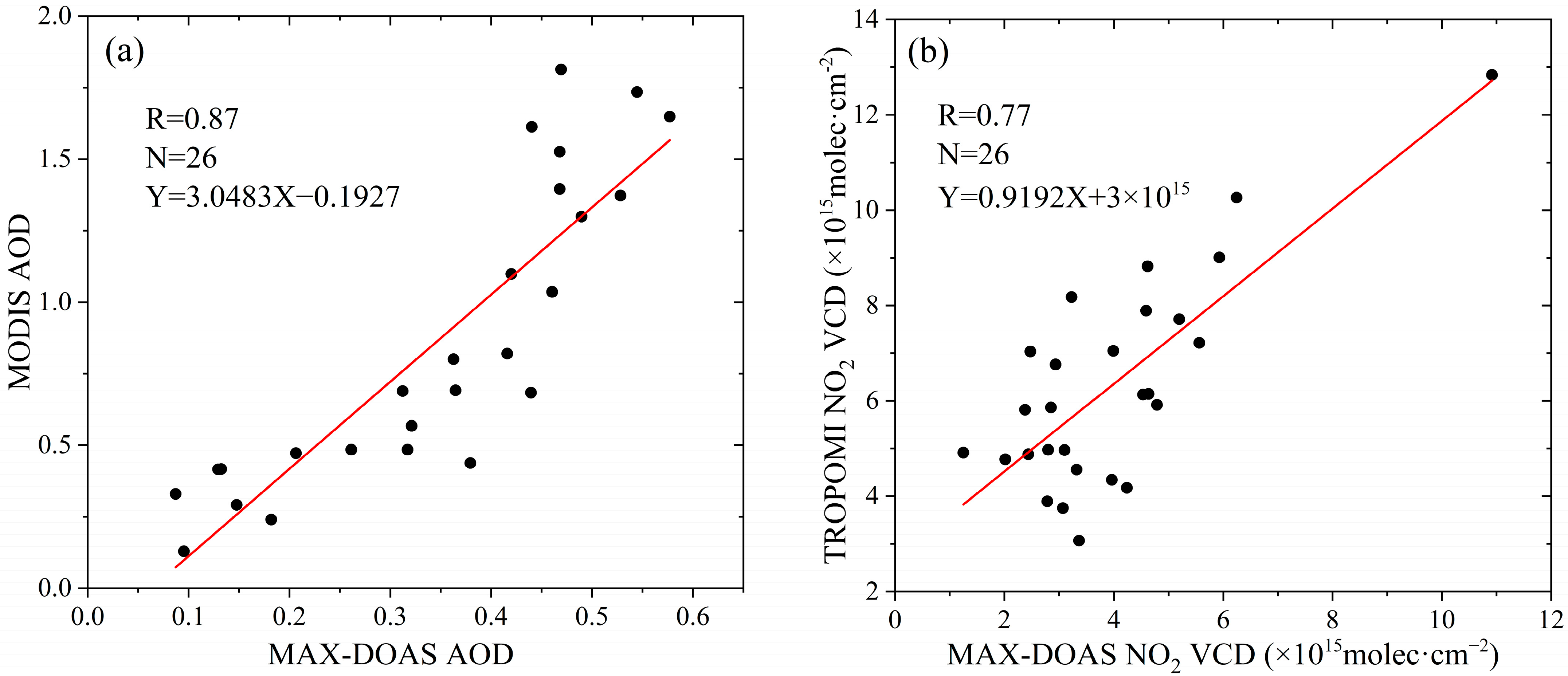
The average AOD at 360.8 nm measured by MAX-DOAS between 10:30 and 13:30 local time was selected for correlation verification with AOD measured by MODIS. The AOD at 360.8 nm from MODIS is derived by calculating the Ångström exponent using the AOD measurements at 470 nm and 550 nm, and then applying this exponent to estimate the AOD at 360.8 nm [81,82]. The results indicated a strong correlation between MAX-DOAS and MODIS AOD, with a correlation coefficient of 0.87 (Figure 3a). Similarly, the average NO₂ VCD measured by MAX-DOAS between 13:20 and 13:40 local time was selected for correlation verification with NO₂ VCD measured by TROPOMI. The results showed a strong correlation between MAX-DOAS and TROPOMI NO₂ VCD, with a correlation coefficient of 0.77 (Figure 3b). The comparison results demonstrated that the data observed by MAX-DOAS were reliable.

3.2. Measurement Overview

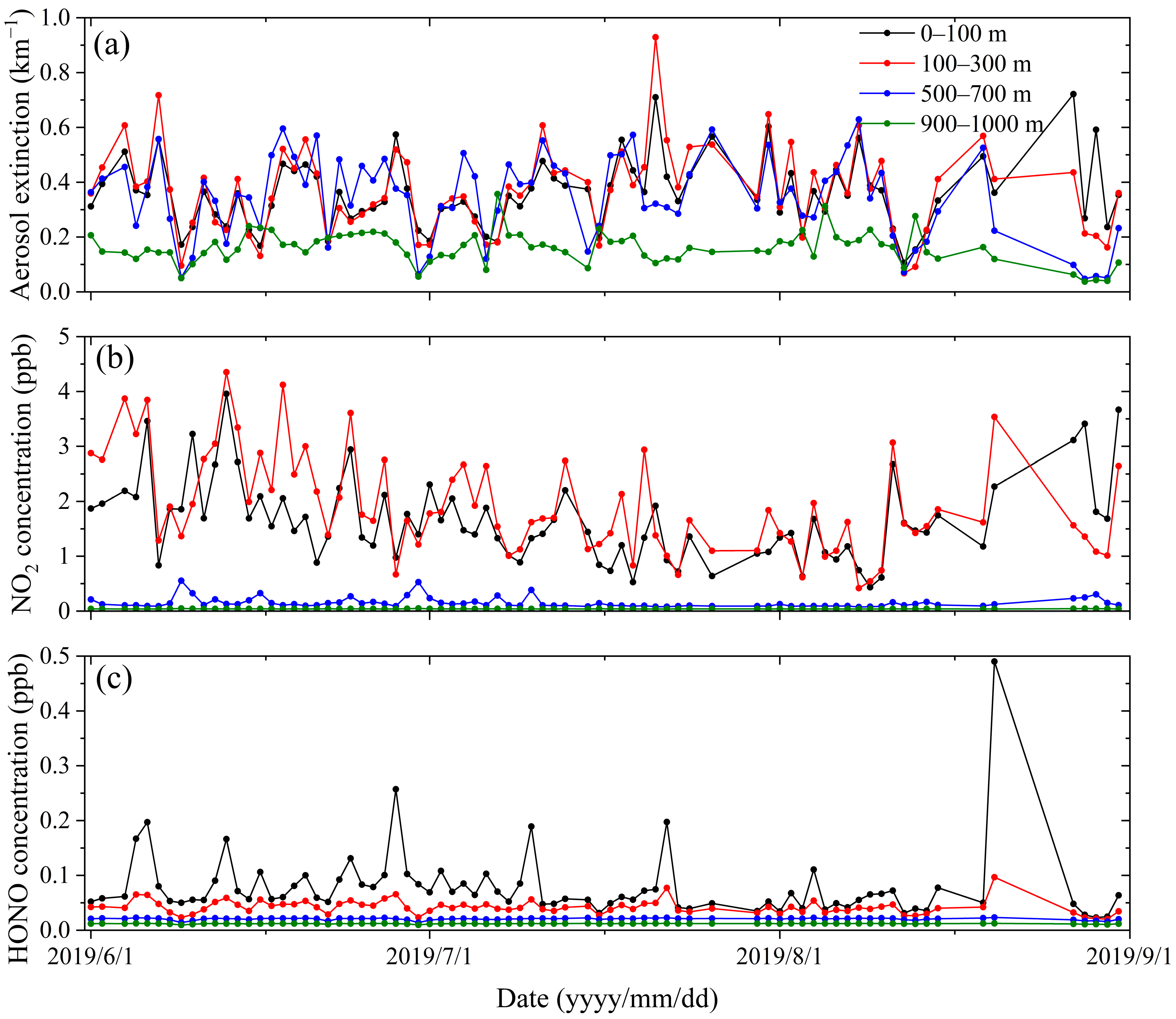
In this study, in order to discuss the vertical distribution characteristics of aerosols, NO₂, and HONO during the summer, four typical altitudes ranges were selected: (1) 0–100 m, representing the bottom boundary layer; (2) 100–300 m, representing the lower boundary layer; (3) 500–700 m, representing the middle boundary layer; and (4) 900–1100 m, representing the upper boundary layer. Time series of trace gases (NO₂ and HONO) and aerosol extinction in the bottom, lower, middle, and upper layers are shown in Figure 4. The average and maximum values (aerosol extinction, NO₂ and HCHO concentration) are presented in

Table 2. The average and maximum concentrations of NO₂, HONO, and aerosol extinction coefficient.

Pollutants	Average Extinction Coefficient (km−1) or Concentration (ppb)				Maximum Extinction Coefficient (km−1) or Concentration (ppb)
	Surface	Lower Layer	Middle Layer	Upper Layer	Surface	Lower Layer	Middle Layer	Upper Layer
Aerosol	0.358	0.370	0.342	0.161	0.722	0.929	0.629	0.357
NO2	1.659	1.926	0.150	0.040	3.958	4.353	0.554	0.049
HONO	0.079	0.042	0.021	0.012	0.490	0.097	0.023	0.013

. During the observation period, the time series of meteorological information (including boundary layer height, temperature, relative humidity, and visibility) in the Wangdu area is shown in Figure S2. The scatter plots between meteorological information (RH and temperature) and pollutants (aerosols, NO₂, HONO, and NO₂/HONO) are shown in Figure S3.

The results showed that NO₂ was mainly distributed in the bottom layer (1.659 ppb) and lower layer (1.926 ppb), with the concentration in the lower layer slightly higher than that in the bottom layer. Compared to the bottom layer, the ratios of NO₂ concentration in the lower, middle, and upper layers were 116.12%, 9.07%, and 2.44%, respectively. Aerosol extinction in the bottom layer (0.358 km⁻¹), lower layer (0.370 km⁻¹), and middle layer (0.342 km⁻¹) was approximately equal and higher than that in the upper layer (0.161 km⁻¹). Compared to the bottom layer, the ratios of aerosol extinction in the lower, middle, and upper layers were 103.47%, 95.67%, and 44.97%, respectively. Unlike aerosols and NO₂, the HONO concentration varied significantly in the four layers, with the highest concentration in the bottom layer (0.079 ppb) and the lowest concentration in the upper layer (0.012 ppb). Compared to the bottom layer, the ratios of HONO concentration in the lower, middle, and upper layers were 53.39%, 26.25%, and 15.20%, respectively. Similar HONO vertical gradients were observed in Colorado using a mass spectrometer on the tower [31], in Los Angeles and Houston using LP-DOAS [35,36], and in Melbourne using MAX-DOAS [37].

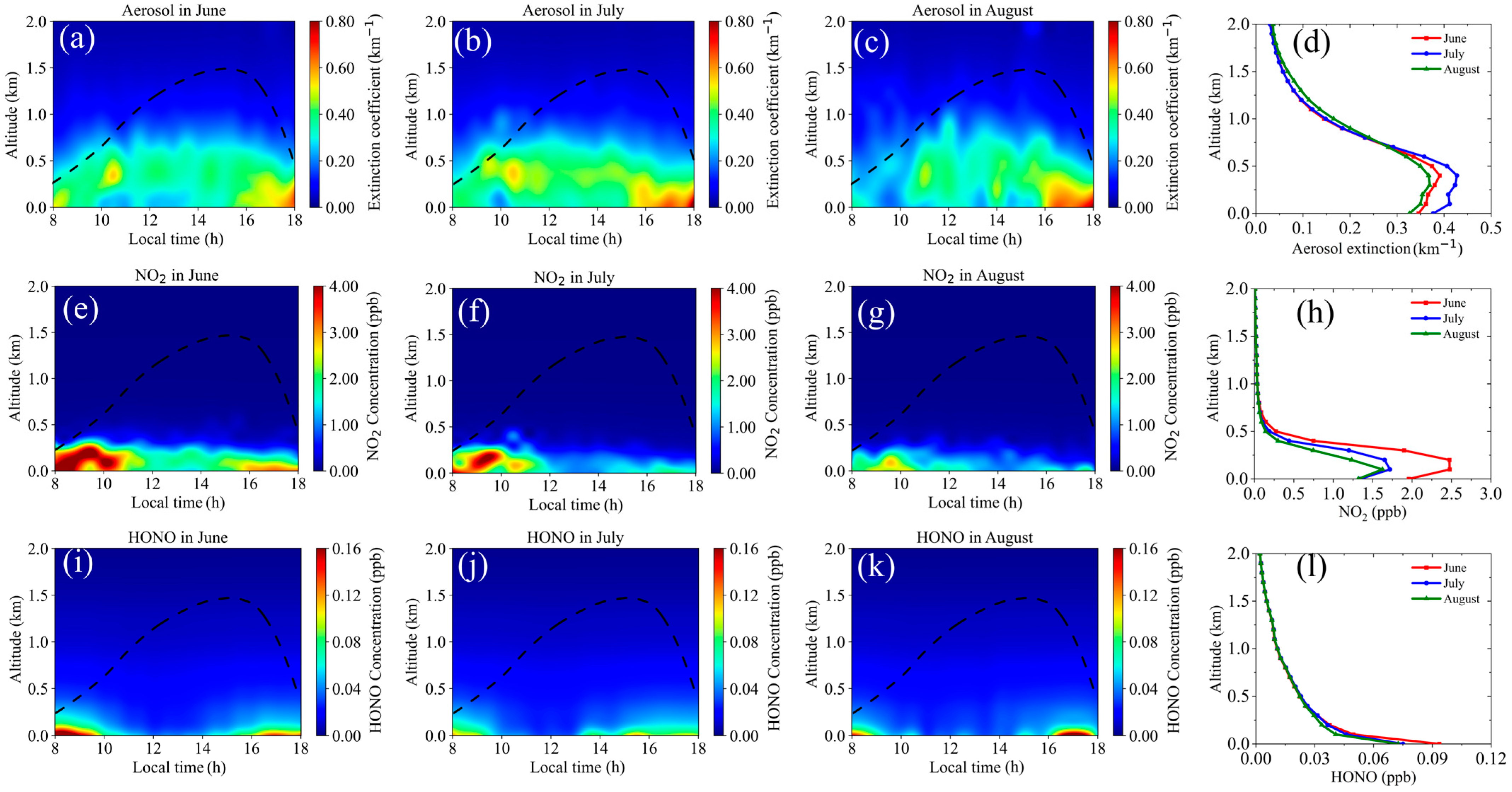
Figure 5 illustrates the diurnal variations in the vertical distributions of aerosol extinction, NO₂, and HONO observed during the study period, along with the corresponding boundary layer height. In the Wangdu area, the boundary layer height reached its peak at noon and was at its lowest during the morning and evening, with an average boundary layer height of 1064 m during the day. This boundary layer height plays a significant role in shaping the diurnal variations of pollutant concentration [83]. The average aerosol extinction near the surface varied in the order of July (0.377 km⁻¹) > August (0.346 km⁻¹) > June (0.343 km⁻¹), slightly higher than the level observed at the nearby rural site of Raoyang (aerosol extinction: 0.33 km⁻¹ during the summer of 2014) [84]. The average NO₂ concentration near the surface varied in the order of June (1.958 ppb) > July (1.341 ppb) > August (1.317 ppb). The average HONO concentration near the surface varied in the order of June (0.094 ppb) > July (0.075 ppb) > August (0.073 ppb).

The vertical profiles of NO₂ and aerosol extinction exhibited a near-Gaussian pattern, characterized by an initial increase in concentration and followed by a decrease with altitude during the summer months. The maximum aerosol extinction was observed around 0.4 km, and the aerosol extinction decreased with the increase in altitude beyond 0.4 km. The maximum NO₂ concentration was observed around 0.15 km, and the NO₂ concentration decreased with the increase in altitude beyond 0.4 km. These trends could be related to the transportation of pollutants. Unlike aerosols and NO₂, the maximum HONO concentration consistently occurred near the surface during different summer months. In addition, HONO concentration decreased exponentially with altitude. Above an altitude of 1 km, the HONO concentration was less than 10% of that near the surface. Similar vertical distributions of HONO have been found in previous studies [1,5,31,44,77].

Similar aerosol diurnal variation characteristics were observed during different months. The maximum aerosol extinction occurred near the surface at 8:00. Subsequently, the altitude of maximum aerosol extinction rose with the increasing boundary layer height, peaking at an altitude of 0.5 km at around 10:00. Between 10:30 and 16:00, the distribution of aerosol concentration at various altitudes exhibited a stable pattern, with the maximum altitude consistently observed at 0.5 km. After 16:00, aerosol extinction decreased with the decrease in the atmospheric boundary layer, concentrating at lower altitudes. By around 18:00, the maximum aerosol extinction for the day occurred at an altitude of approximately 0.1 km.

In June, July, and August, the maximum concentrations of NO₂ were found at 8:00, 9:00, and 10:00, respectively, showing significant variation characteristics. The peak of NO₂ concentrations appeared at 8:00–10:00 and 16:00–18:00. The minimum NO₂ concentration appeared at noon, which might be related to the photolysis of NO₂ [85]. In addition, the rise of the boundary layer at noon also facilitated the vertical diffusion of NO₂ [39]. After 16:00, the reduction in boundary layer height led to an accumulation of NO₂ at ground level, resulting in the formation of a secondary peak. Similar diurnal variations have been previously observed in the Wangdu area [86].

The highest concentration of HONO was observed near the surface at 8:00 across all months. This phenomenon can be attributed to the decline in solar radiation after sunset, which reduced the photolytic loss of HONO. Additionally, heterogeneous reactions of NO₂ led to the accumulation of HONO during the night, reaching its maximum concentration in the early morning [25,31,44,77]. After sunrise, HONO concentration decreased rapidly due to photolysis, remaining a low concentration from 10:00 to 14:00. After 16:00, HONO concentration increased with the rise in the precursor NO₂ concentration and the decrease in sunlight, reaching a second peak near the surface. Similar HONO diurnal variation characteristics were also found in farmland environment studies Wangdu [27] and Xingtai [51] in the North China Plain, China, as well as in Cabauw, the Netherlands [87], and Grignon, France [88].

3.3. The Difference of Aerosol, NO₂, and HONO Profiles during Non-Haze and Haze Days

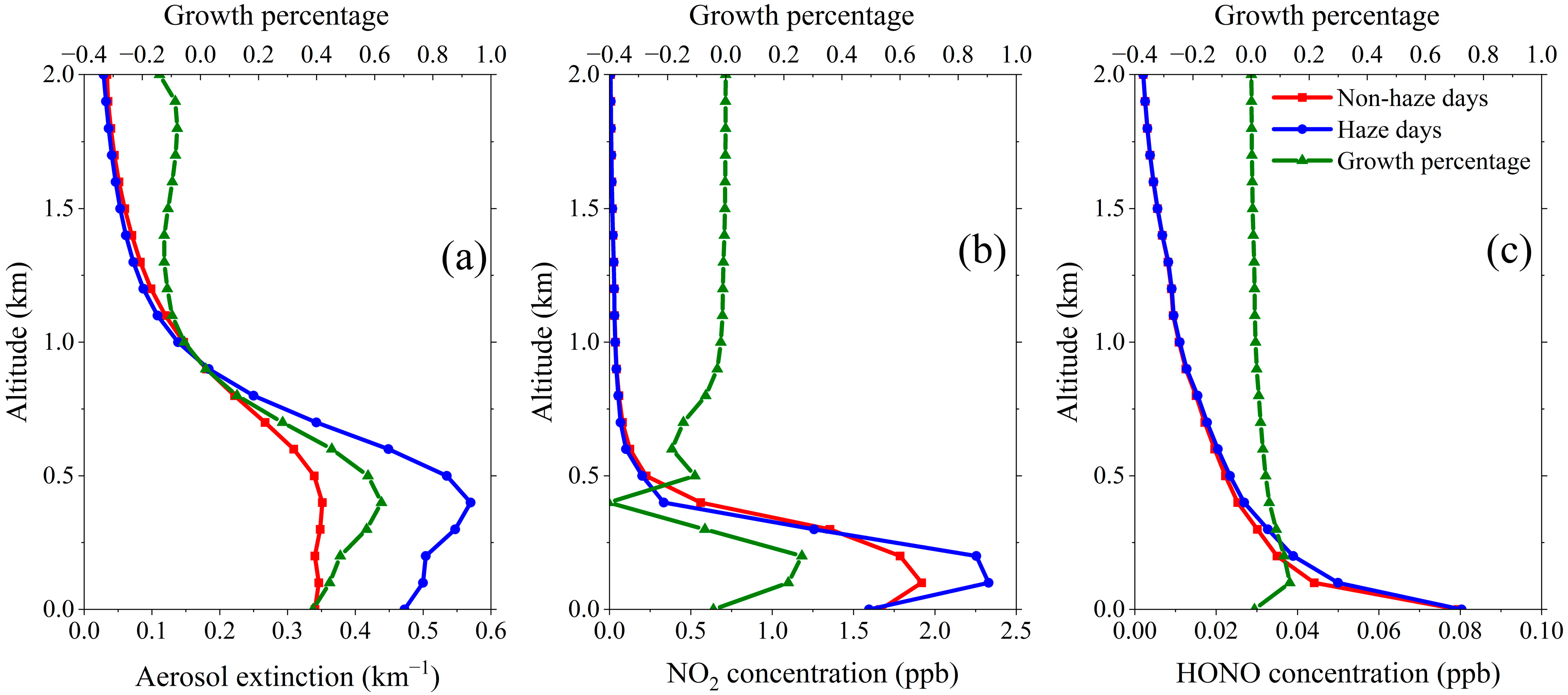
To assess the impact of haze on pollutants, the profiles of aerosol, NO₂, and HONO during non-haze and haze days are shown in Figure 6, with the corresponding error bars illustrated in Figure S5.

As shown in Figure 6, the average profile shapes of aerosols, NO₂, and HONO were generally similar on both non-haze and haze days. Aerosols and NO₂ exhibited a near-Gaussian distribution, while HONO showed an exponential decrease with altitude. During non-haze days, within the 0–0.4 km altitude range, the average aerosol extinction, NO₂ concentration, and HONO concentration were 0.345 km⁻¹, 1.457 ppb, and 0.043 ppb, respectively. During haze days, within the same altitude range, the average aerosol extinction, NO₂ concentration, and HONO concentration were 0.519 km⁻¹, 1.554 ppb, and 0.046 ppb, respectively. The aerosol extinction on haze days was significantly higher than that on non-haze days, likely due to the increased conversion of directly emitted pollutants into secondary pollutants [9,24,89]. The NO₂ and HONO concentrations were slightly higher on haze days compared to non-haze days. On haze days, the higher aerosol concentration enhanced heterogeneous reactions on aerosol surfaces, leading to an increase in HONO concentration [90]. Additionally, the weaker sunlight on haze days prevented the photolysis of NO₂, resulting in higher NO₂ concentrations [91].

To further quantify the differences in the vertical distribution of pollutants between non-haze and haze days at different altitudes, the growth percentages of atmospheric pollutants were calculated. As shown in Figure 6, the highest growth percentage of aerosol occurred at 0.4 km, approximately 62%, and decreased with altitude above 0.4 km, reaching approximately zero above 0.9 km. This indicated that aerosol pollution on haze days mainly occurred at mid-altitude and low-altitude layers. The highest growth percentages of NO₂ were observed at altitudes of 0.1 km and 0.2 km, approximately 21% and 26%, respectively. A negative growth percentage of approximately −40% was observed at 0.4 km. The highest growth percentage of HONO occurred at an altitude of 0.1 km, approximately 13%, and decreased slowly with altitude above 0.1 km. Compared to aerosols and NO₂, the growth percentage of HONO is much smaller, indicating that haze exerts a lesser influence on HONO levels.

3.4. Aerosols and NO₂ Potential Sources in Agricultural Regions in Summer

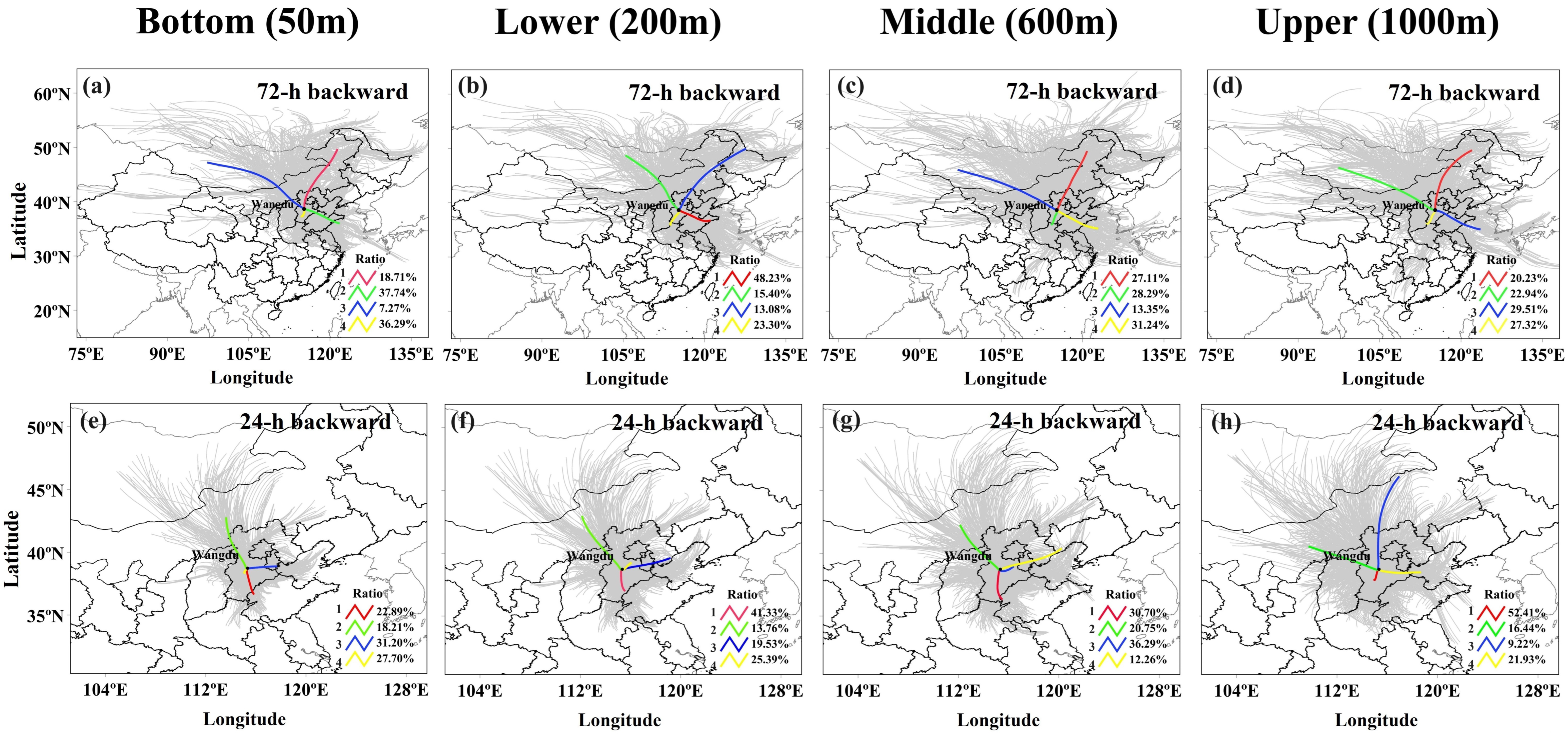
The observation station is located in farmland with no apparent emission sources nearby. To further elucidate the potential sources of aerosols and NO₂ at the station and to assess transport influences, we calculated the backward trajectories of the air mass at the bottom boundary layer (50 m), lower boundary layer (200 m), middle boundary layer (600 m), and upper boundary layer (1000 m) arriving at Wangdu station in the summer of 2019. Due to the different lifetimes of atmospheric pollutants, 72 h and 24 h backward trajectories were calculated for aerosols and NO₂, respectively, with a time interval of 1 h.

Figure 7 and

Table 3. Trajectory ratios and averages of aerosol extinction coefficient (corresponding to the 72 h backward trajectories) and NO₂ concentration (corresponding to the 24 h backward trajectories) for all trajectory clusters arriving at Wangdu at bottom (50 m), lower (200 m), middle (600 m), and upper (1000 m) in the summer of 2019.

	Cluster	Traj_Ratio	Aerosol Extinction (km−1)	Cluster	Traj_Ratio	NO2 (ppb)
			Mean ± S.D.			Mean ± S.D.
Bottom (50 m)	1	18.71%	0.262 ± 0.045	1	22.89%	1.745 ± 0.262
	2	37.74%	0.356 ± 0.062	2	18.21%	1.898 ± 0.325
	3	7.24%	0.429 ± 0.081	3	31.20%	1.859 ± 0.258
	4	36.29%	0.405 ± 0.068	4	27.70%	1.967 ± 0.313
	All	100%	0.358 ± 0.062	All	100%	1.873 ± 0.281
Lower (200 m)	1	48.23%	0.419 ± 0.063	1	41.33%	2.098 ± 0.304
	2	15.40%	0.247 ± 0.040	2	13.76%	1.527 ± 0.159
	3	13.08%	0.172 ± 0.032	3	19.53%	2.278 ± 0.302
	4	23.30%	0.501 ± 0.102	4	25.39%	2.236 ± 0.426
	All	100%	0.378 ± 0.058	All	100%	2.091 ± 0.307
Middle (600 m)	1	27.11%	0.190 ± 0.028	1	30.70%	0.117 ± 0.020
	2	28.29%	0.367 ± 0.055	2	20.75%	0.192 ± 0.035
	3	13.35%	0.263 ± 0.042	3	36.29%	0.118 ± 0.017
	4	31.24%	0.377 ± 0.062	4	12.26%	0.143 ± 0.031
	All	100%	0.315 ± 0.045	All	100%	0.137 ± 0.026
Upper (1000 m)	1	20.23%	0.108 ± 0.017	1	52.41%	0.040 ± 0.006
	2	22.94%	0.108 ± 0.016	2	16.44%	0.041 ± 0.018
	3	29.51%	0.174 ± 0.021	3	9.22%	0.042 ± 0.013
	4	27.32%	0.129 ± 0.020	4	21.93%	0.040 ± 0.021
	All	100%	0.138 ± 0.019	All	100%	0.040 ± 0.015

, respectively, summarize the clustering pathways and clustering characteristics in the bottom layer (50 m), lower layer (200 m), middle layer (600 m), and upper layer (1000 m) at Wangdu station during the observation period. For aerosols (Figure 7a–d), the maximum aerosol extinction was reached in Cluster 3 (0.429 ± 0.081 km⁻¹) at 50 m, Cluster 4 (0.501 ± 0.102 km⁻¹) at 200 m, Cluster 4 (0.377 ± 0.062 km⁻¹) at 600 m, and Cluster 3 (0.174 ± 0.021 km⁻¹) at 1000 m. Cluster 3 at 50 m represented long-distance trajectories from the Inner Mongolia Plateau. Cluster 4 at 200 m was a short track from the border of Shanxi and Hebei. Cluster 4 at 600 m and Cluster 3 at 1000 m originated from the Yellow Sea and passed through Shandong province into Hebei province. For NO₂ (Figure 7e–h), the maximum concentrations were found in Cluster 4 (1.967 ± 0.313 ppb) at 50 m, Cluster 3 (2.278 ± 0.302 ppb) at 200 m, Cluster 2 (0.192 ± 0.035 ppb) at 600 m, and Cluster 3 (0.042 ± 0.013 ppb) at 1000 m. Among them, Cluster 4 at 50 m was a short-distance transmission, originating from central Hebei province. Cluster 3 at 200 m originated from the Bohai Sea coast and passed through Tianjin province, similar to the cluster observed at the nearby Gucheng site [92]. These results indicated that short-range transport from central Hebei and mid-range transport from the Bohai Sea coast significantly impacted the NO₂ pollution at Wangdu station.

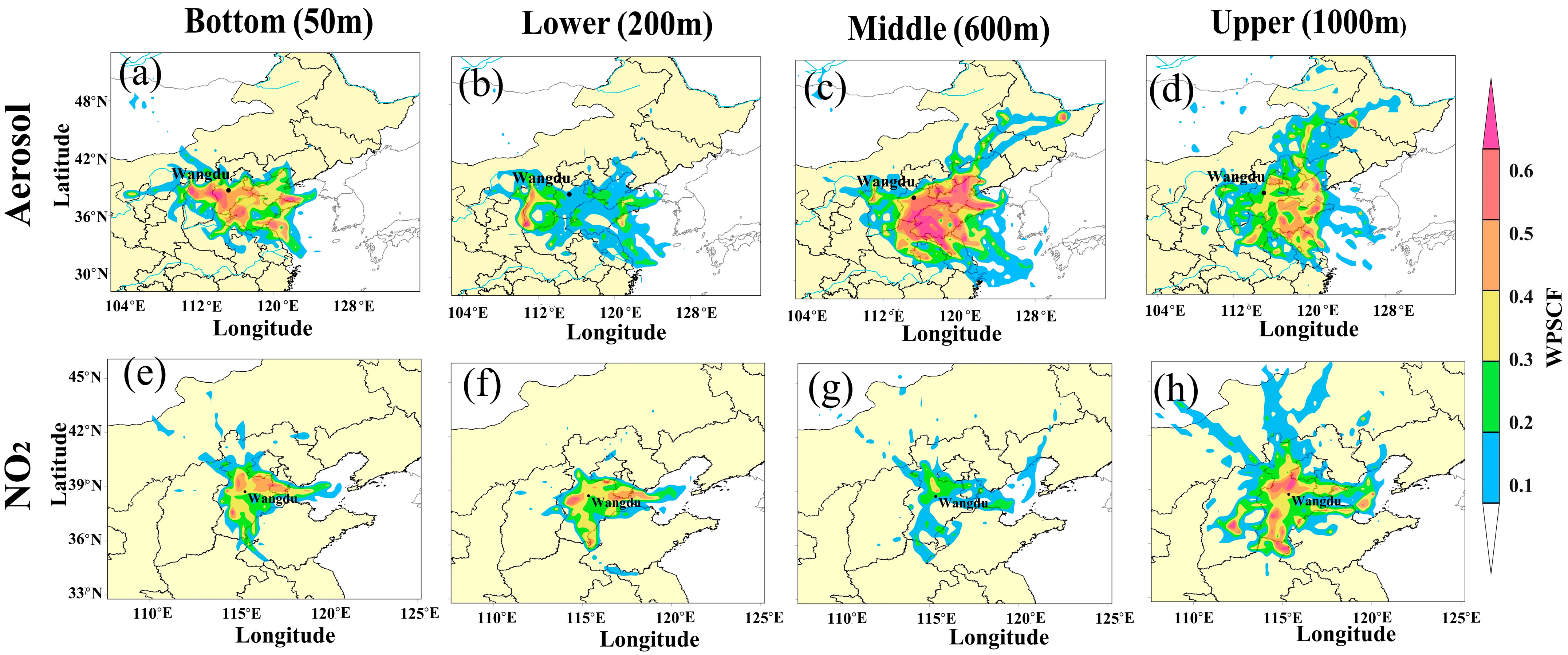
In addition, the WPSCF values of aerosol and NO₂ were analyzed at different altitudes to characterize potential pollutant sources. A higher WPSCF value indicated a more significant contribution of pollutants from the region to the observation station. In this study, regions with WPSCF values between 0.3 and 0.4 were defined as having low pollution contribution, between 0.4 and 0.5 as middle pollution contribution, and WPSCF values greater than 0.5 as high pollution contribution regions [93,94].

As shown in Figure 8, pollutants at different altitudes generally originated from the same source directions, but potential pollution sources were more widely distributed in mid- to high-altitude regions compared to low-altitude areas, with similar phenomena also observed in Xingtai [51]. High pollution contribution regions for aerosol were mainly distributed in the Shanxi, Shandong, and Jiangsu provinces and the southern part of Hebei province. The predominant potential aerosol source below 200 m was Shanxi province, known for its abundant coal resources, where coal combustion and biomass burning significantly contribute to PM_2.5 emissions [95]. Above 500 m, aerosols primarily originated from the southeast, especially in the Shandong and Jiangsu provinces. High pollution contribution regions for NO₂ were mainly distributed in the Beijing–Tianjin–Hebei region, due to heavy industrial emissions. The combustion of fossil fuels in heavy industries was an important source of NO₂ emissions [96]. In addition, Beijing and Tianjin, with high population densities and heavy traffic flow, contributed to high NO₂ concentrations [97,98]. In the high-altitude region above 1000 m, the southern part of Shanxi and the Bohai Sea were also high pollution contribution regions for NO₂.

3.5. Heterogeneous Contribution to HONO from NO₂ in Agricultural Regions in Summer

The heterogeneous reactions of NO₂ on wet surfaces are also an important source of HONO. Data indicating an increase in the ratio of HONO to NO₂ over a continuous three-hour period between 8:00 and 18:00 were used to calculate the conversion rate from NO₂ to HONO.

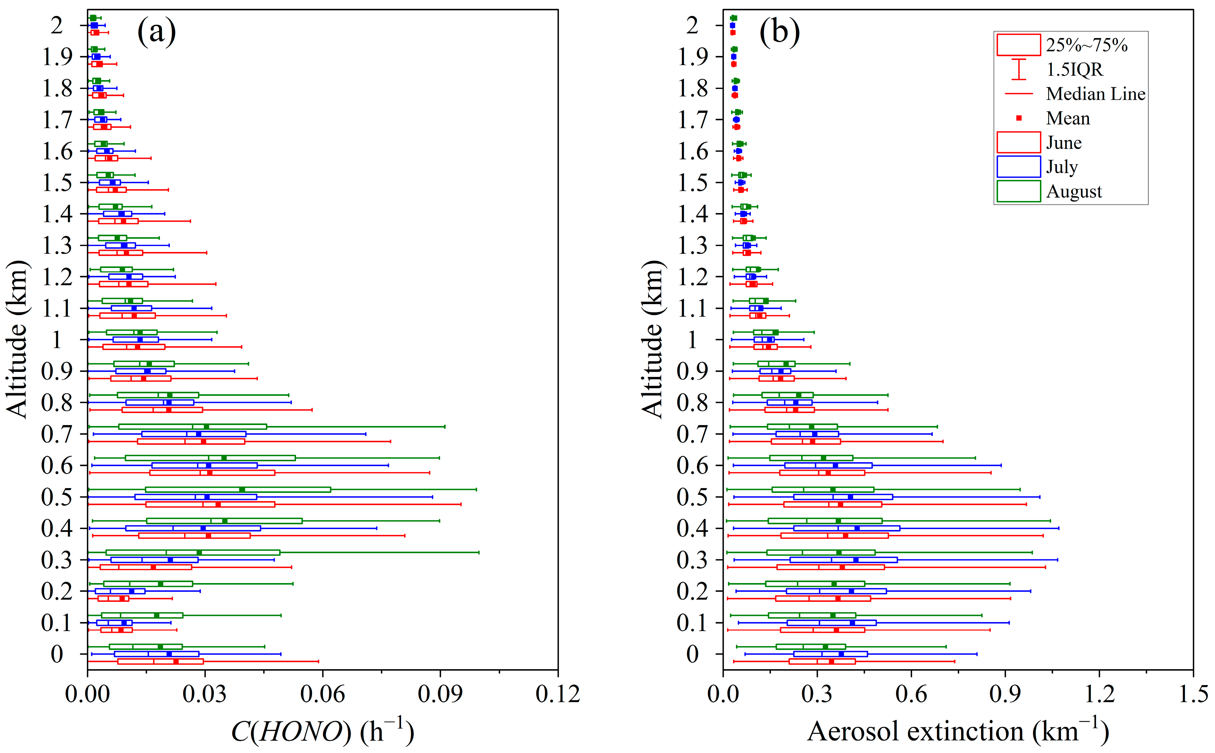
Figure 9 describes the variation of $C\left(HONO\right)$ and the aerosol extinction coefficient with altitude during the summer months. Table S2 shows the monthly average temperature and humidity during the summer. We found that the mean $C\left(HONO\right)$ near the surface varied in the order of June (0.0226 h⁻¹) > July (0.0208 h⁻¹) > August (0.0186 h⁻¹). $C\left(HONO\right)$ decreased with altitude between 0 and 150 m, reaching the first low point at 150 m. This may be attributed to the neglect of HONO emissions from agricultural sources, leading to an overestimation of near-surface $C\left(HONO\right)$ [66]. $C\left(HONO\right)$ increased with altitude from 150 m to 500 m. The maximum mean $C\left(HONO\right)$ occurred at 500 m, varying in the order of August (0.0395 h⁻¹) > June (0.0333 h⁻¹) > July (0.0324 h⁻¹). $C\left(HONO\right)$ continued to decrease with altitude above 500 m. The minimum mean $C\left(HONO\right)$ occurred at the highest altitude of 2000 m, varying in the order of June (0.0022 h⁻¹) > July (0.0018 h⁻¹) > August (0.0015 h⁻¹). The maximum aerosol extinction also occurred near 500 m and decreased continuously with altitude above 500 m, consistent with the trend of $C\left(HONO\right)$.

3.6. OH Radicals Produced from HONO Photolysis at Different Altitudes

HONO photolysis is one of the important sources of atmospheric OH radicals, affecting the atmospheric oxidation capacity [2,10]. To evaluate the role of HONO in the production of OH radicals in agricultural regions, the photolysis frequency of HONO and its contribution to the OH generation rate were determined using the TUV model.

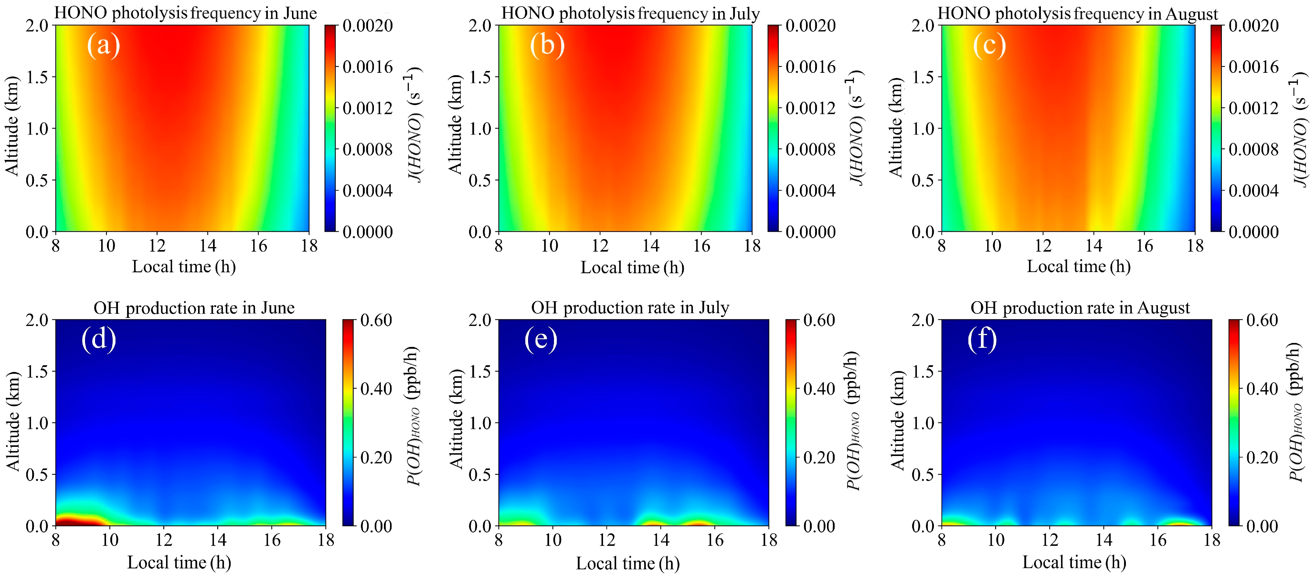
The TUV model performs best on cloudless and non-haze days, so data on such days were selected for analysis. The monthly average HONO photolysis frequency and OH generation rate during the observation period are shown in Figure 10. The average HONO photolysis frequency near the surface varied in the order of June (0.00124 s⁻¹) > July (0.00122 s⁻¹) > August (0.00115 s⁻¹). The HONO photolysis frequency increased with altitude, typically reaching its peak around 12:00 to 13:00 daily. In contrast to the trend of photolysis frequency, the OH production rate decreased with altitude, with peaks occurring in the morning and late afternoon.

4. Discussion

In the time series of trace gases in Wangdu (Figure 4), we observed a peak in HONO concentrations on 20 August, reaching approximately 0.49 ppb, even though the NO₂ levels on that day were not high. Further analysis of the diurnal variation in HONO on 20 August, as shown in Figure S5, indicated that high levels of HONO occurred in the morning (8:00–9:00), at noon (11:00–13:00), and in the evening (16:00–18:00). Similar diurnal variation patterns were observed at the same site (Wangdu) during the fertilization period [99]. Therefore, we suspect this phenomenon may be related to local agricultural activities.

The peak levels of NO₂ occurred at 8:00–10:00 and 16:00–18:00 (Figure 5e–g), even though the station is located in an agricultural area. This is consistent with previous observations in the rural areas of Gucheng [92] and Raoyang [100] in the NCP. On the one hand, despite being situated in an agricultural area, the observation site experienced significant NO₂ emissions from a major highway located nearby to the northwest (Figure S6). Moreover, weak photolysis of NO₂ during the night led to an accumulation of NO₂ after sunset, resulting in peak concentrations in the morning [85]. On the other hand, the low boundary layer in the morning and evening hindered the diffusion of NO₂ [39].

Above 500 m, the trend of the $C\left(HONO\right)$ profile was consistent with aerosols (Figure 9). It can be inferred that above 500 m, heterogeneous reactions on aerosol surfaces were one of the important HONO sources. Furthermore, we analyzed the correlation between the ratio of HONO to NO₂ and aerosols at different altitudes, with the results shown in Figure S7. The results indicate that the correlation between the ratio of HONO to NO₂ and aerosols above 500 m was significantly stronger than that below 500 m, further supporting this inference.

The production and loss of OH may involve complex chemical reactions, such as the photolysis of O₃ and HCHO leading to OH formation [101], and the homogeneous reaction between OH and NO resulting in OH loss [102]. This study aims to provide a preliminary quantitative analysis of the relationship between OH production from photolysis, HONO concentration, and photolysis rates, with a particular focus on the contribution of HONO to atmospheric OH levels. The summer average OH production rate near the surface was 0.297 ppb/h, slightly higher than that reported in the urban regions of Hefei (0.287 ppb/h) and lower than that in the rural regions of Hefei (0.36 ppb/h) [66]. The maximum OH production rate near the surface in summer was 0.872 ppb/h, slightly higher than that in Beijing (approximately 0.700 ppb/h) [5]. The OH production rate decreased with altitude, with peaks in the morning and late afternoon, consistent with the variation in HONO concentration, contrary to the HONO photolysis rate. This trend indicated that the OH production rate from HONO photolysis was mainly controlled by HONO concentration.

5. Conclusions

MAX-DOAS observations were conducted in the agricultural regions of the NCP to measure vertical distributions of aerosols, NO₂, and HONO. MAX-DOAS NO₂ VCD and AOD showed correlations of 0.77 and 0.87, respectively, with TROPOMI NO₂ VCD and MODIS AOD. The vertical profiles of aerosols and NO₂ exhibited a near-Gaussian distribution. Aerosol extinction peaked typically before 10:00 in the morning and after 17:00, influenced by diurnal variations in the boundary layer height. NO₂ peaks appeared at 8:00–10:00 and 16:00–18:00. HONO reached its maximum concentration near the surface around 8:00 due to nighttime accumulation and exponentially decreased with height. After sunrise, HONO concentration rapidly reduced due to photolysis.

Potential source analysis suggested that the main potential sources of aerosol pollution were in the southern part of the Hebei, Shanxi, Shandong, and Jiangsu provinces. The primary potential pollution sources for NO₂ were in the Beijing–Tianjin–Hebei region. The south of Shanxi province and the Bohai Sea area were also significant potential pollution sources for NO₂ above 1000 m. Additionally, the NO₂ to HONO conversion rate through heterogeneous reactions was calculated, revealing that the maximum values of C(HONO) and aerosol extinction occurred near 500 m, and decreased continuously with altitude above 500 m. This suggested that the heterogeneous reactions of NO₂ on aerosol surfaces play a significant role as sources of HONO at altitudes above 500 m.

HONO serves as a crucial source of OH in the atmosphere. In this study, we observed that the maximum photolysis frequency of HONO consistently occurred between 12:00 and 13:00 each day. The production rate of OH from HONO photolysis exhibited a decrease with altitude, with peaks occurring in the morning and late afternoon, which correlated with the variation in HONO concentration. This indicated that the OH production rate was primarily controlled by HONO concentration.

References

- Garcia-Nieto, D.; Benavent, N.; Saiz-Lopez, A. Measurements of Atmospheric HONO Vertical Distribution and Temporal Evolution in Madrid (Spain) Using the MAX-DOAS Technique. Sci. Total Environ. 2018, 643, 957–966. [Google Scholar] [CrossRef] [PubMed]
- Huang, R.-J.; Yang, L.; Cao, J.; Wang, Q.; Tie, X.; Ho, K.-F.; Shen, Z.; Zhang, R.; Li, G.; Zhu, C.; et al. Concentration and Sources of Atmospheric Nitrous Acid (HONO) at an Urban Site in Western China. Sci. Total Environ. 2017, 593–594, 165–172. [Google Scholar] [CrossRef]
- Michoud, V.; Kukui, A.; Camredon, M.; Colomb, A.; Borbon, A.; Miet, K.; Aumont, B.; Beekmann, M.; Durand-Jolibois, R.; Perrier, S.; et al. Radical Budget Analysis in a Suburban European Site during the MEGAPOLI Summer Field Campaign. Atmos. Chem. Phys. 2012, 12, 11951–11974. [Google Scholar] [CrossRef]
- Perner, D.; Platt, U. Detection of Nitrous Acid in the Atmosphere by Differential Optical Absorption. Geophys. Res. Lett. 1979, 6, 917–920. [Google Scholar] [CrossRef]
- Hendrick, F.; Müller, J.-F.; Clémer, K.; Wang, P.; De Mazière, M.; Fayt, C.; Gielen, C.; Hermans, C.; Ma, J.Z.; Pinardi, G.; et al. Four Years of Ground-Based MAX-DOAS Observations of HONO and NO2 in the Beijing Area. Atmos. Chem. Phys. 2014, 14, 765–781. [Google Scholar] [CrossRef]
- Su, H.; Cheng, Y.F.; Cheng, P.; Zhang, Y.H.; Dong, S.; Zeng, L.M.; Wang, X.; Slanina, J.; Shao, M.; Wiedensohler, A. Observation of Nighttime Nitrous Acid (HONO) Formation at a Non-Urban Site during PRIDE-PRD2004 in China. Atmos. Environ. 2008, 42, 6219–6232. [Google Scholar] [CrossRef]
- Acker, K.; Möller, D.; Wieprecht, W.; Meixner, F.X.; Bohn, B.; Gilge, S.; Plass-Dülmer, C.; Berresheim, H. Strong Daytime Production of OH from HNO2 at a Rural Mountain Site. Geophys. Res. Lett. 2006, 33, L02809. [Google Scholar] [CrossRef]
- Song, Y.; Zhang, Y.; Xue, C.; Liu, P.; He, X.; Li, X.; Mu, Y. The Seasonal Variations and Potential Sources of Nitrous Acid (HONO) in the Rural North China Plain. Environ. Pollut. 2022, 311, 119967. [Google Scholar] [CrossRef]
- Huang, R.-J.; Zhang, Y.; Bozzetti, C.; Ho, K.-F.; Cao, J.-J.; Han, Y.; Daellenbach, K.R.; Slowik, J.G.; Platt, S.M.; Canonaco, F.; et al. High Secondary Aerosol Contribution to Particulate Pollution during Haze Events in China. Nature 2014, 514, 218–222. [Google Scholar] [CrossRef] [PubMed]
- Lelieveld, J.; Dentener, F.J.; Peters, W.; Krol, M.C. On the Role of Hydroxyl Radicals in the Self-Cleansing Capacity of the Troposphere. Atmos. Chem. Phys. 2004, 4, 2337–2344. [Google Scholar] [CrossRef]
- Jarvis, D.L.; Leaderer, B.P.; Chinn, S.; Burney, P.G. Indoor Nitrous Acid and Respiratory Symptoms and Lung Function in Adults. Thorax 2005, 60, 474–479. [Google Scholar] [CrossRef]
- Ohyama, M.; Nakajima, T.; Minejima, C.; Azuma, K.; Oka, K.; Itano, Y.; Kudo, S.; Takenaka, N. Association between Indoor Nitrous Acid, Outdoor Nitrogen Dioxide, and Asthma Attacks: Results of a Pilot Study. Int. J. Environ. Health Res. 2019, 29, 632–642. [Google Scholar] [CrossRef] [PubMed]
- Sleiman, M.; Gundel, L.A.; Pankow, J.F.; Jacob, P.; Singer, B.C.; Destaillats, H. Formation of Carcinogens Indoors by Surface-Mediated Reactions of Nicotine with Nitrous Acid, Leading to Potential Thirdhand Smoke Hazards. Proc. Natl. Acad. Sci. USA 2010, 107, 6576–6581. [Google Scholar] [CrossRef]
- Ge, M.; Tong, S.; Wang, W.; Zhang, W.; Chen, M.; Peng, C.; Li, J.; Zhou, L.; Chen, Y.; Liu, M. Important Oxidants and Their Impact on the Environmental Effects of Aerosols. J. Phys. Chem. A 2021, 125, 3813–3825. [Google Scholar] [CrossRef] [PubMed]
- Li, X.; Brauers, T.; Häseler, R.; Bohn, B.; Fuchs, H.; Hofzumahaus, A.; Holland, F.; Lou, S.; Lu, K.D.; Rohrer, F.; et al. Exploring the Atmospheric Chemistry of Nitrous Acid (HONO) at a Rural Site in Southern China. Atmos. Chem. Phys. 2012, 12, 1497–1513. [Google Scholar] [CrossRef]
- Su, H.; Cheng, Y.F.; Shao, M.; Gao, D.F.; Yu, Z.Y.; Zeng, L.M.; Slanina, J.; Zhang, Y.H.; Wiedensohler, A. Nitrous Acid (HONO) and Its Daytime Sources at a Rural Site during the 2004 PRIDE-PRD Experiment in China. J. Geophys. Res. Atmos. 2008, 113, D14312. [Google Scholar] [CrossRef]
- Calvert, J.G.; Yarwood, G.; Dunker, A.M. An Evaluation of the Mechanism of Nitrous Acid Formation in the Urban Atmosphere. Res. Chem. Intermed. 1994, 20, 463–502. [Google Scholar] [CrossRef]
- Li, S.; Song, W.; Zhan, H.; Zhang, Y.; Zhang, X.; Li, W.; Tong, S.; Pei, C.; Wang, Y.; Chen, Y.; et al. Contribution of Vehicle Emission and NO2 Surface Conversion to Nitrous Acid (HONO) in Urban Environments: Implications from Tests in a Tunnel. Environ. Sci. Technol. 2021, 55, 15616–15624. [Google Scholar] [CrossRef]
- Oswald, R.; Behrendt, T.; Ermel, M.; Wu, D.; Su, H.; Cheng, Y.; Breuninger, C.; Moravek, A.; Mougin, E.; Delon, C.; et al. HONO Emissions from Soil Bacteria as a Major Source of Atmospheric Reactive Nitrogen. Science 2013, 341, 1233–1235. [Google Scholar] [CrossRef]
- Stemmler, K.; Ammann, M.; Donders, C.; Kleffmann, J.; George, C. Photosensitized Reduction of Nitrogen Dioxide on Humic Acid as a Source of Nitrous Acid. Nature 2006, 440, 195–198. [Google Scholar] [CrossRef]
- Han, C.; Yang, W.; Wu, Q.; Yang, H.; Xue, X. Heterogeneous Photochemical Conversion of NO2 to HONO on the Humic Acid Surface under Simulated Sunlight. Environ. Sci. Technol. 2016, 50, 5017–5023. [Google Scholar] [CrossRef]
- Su, H.; Cheng, Y.; Oswald, R.; Behrendt, T.; Trebs, I.; Meixner, F.X.; Andreae, M.O.; Cheng, P.; Zhang, Y.; Pöschl, U. Soil Nitrite as a Source of Atmospheric HONO and OH Radicals. Science 2011, 333, 1616–1618. [Google Scholar] [CrossRef]
- Wang, S.; Zhou, R.; Zhao, H.; Wang, Z.; Chen, L.; Zhou, B. Long-Term Observation of Atmospheric Nitrous Acid (HONO) and Its Implication to Local NO2 Levels in Shanghai, China. Atmos. Environ. 2013, 77, 718–724. [Google Scholar] [CrossRef]
- Cui, L.; Li, R.; Zhang, Y.; Meng, Y.; Fu, H.; Chen, J. An Observational Study of Nitrous Acid (HONO) in Shanghai, China: The Aerosol Impact on HONO Formation during the Haze Episodes. Sci. Total Environ. 2018, 630, 1057–1070. [Google Scholar] [CrossRef] [PubMed]
- Meng, F.; Qin, M.; Fang, W.; Duan, J.; Tang, K.; Zhang, H.; Shao, D.; Liao, Z.; Feng, Y.; Huang, Y.; et al. Measurement of HONO Flux Using the Aerodynamic Gradient Method over an Agricultural Field in the Huaihe River Basin, China. Atmos. Chem. Complex Air Pollut. 2022, 114, 297–307. [Google Scholar] [CrossRef]
- Tang, K.; Qin, M.; Duan, J.; Fang, W.; Meng, F.; Liang, S.; Xie, P.; Liu, J.; Liu, W.; Xue, C.; et al. A Dual Dynamic Chamber System Based on IBBCEAS for Measuring Fluxes of Nitrous Acid in Agricultural Fields in the North China Plain. Atmos. Environ. 2019, 196, 10–19. [Google Scholar] [CrossRef]
- Xue, C.; Ye, C.; Zhang, C.; Catoire, V.; Liu, P.; Gu, R.; Zhang, J.; Ma, Z.; Zhao, X.; Zhang, W.; et al. Evidence for Strong HONO Emission from Fertilized Agricultural Fields and Its Remarkable Impact on Regional O3 Pollution in the Summer North China Plain. ACS Earth Space Chem. 2021, 5, 340–347. [Google Scholar] [CrossRef]
- Meng, F.; Qin, M.; Tang, K.; Duan, J.; Fang, W.; Liang, S.; Ye, K.; Xie, P.; Sun, Y.; Xie, C.; et al. High-Resolution Vertical Distribution and Sources of HONO and NO2 in the Nocturnal Boundary Layer in Urban Beijing, China. Atmos. Chem. Phys. 2020, 20, 5071–5092. [Google Scholar] [CrossRef]
- Acker, K.; Febo, A.; Trick, S.; Perrino, C.; Bruno, P.; Wiesen, P.; Möller, D.; Wieprecht, W.; Auel, R.; Giusto, M.; et al. Nitrous Acid in the Urban Area of Rome. Atmos. Environ. 2006, 40, 3123–3133. [Google Scholar] [CrossRef]
- Gall, E.T.; Griffin, R.J.; Steiner, A.L.; Dibb, J.; Scheuer, E.; Gong, L.; Rutter, A.P.; Cevik, B.K.; Kim, S.; Lefer, B.; et al. Evaluation of Nitrous Acid Sources and Sinks in Urban Outflow. Atmos. Environ. 2016, 127, 272–282. [Google Scholar] [CrossRef]
- VandenBoer, T.; Brown, S.; Murphy, J.; Keene, W.; Young, C.; Pszenny, A.; Kim, S.; Warneke, C.; de Gouw, J.; Maben, J.; et al. Understanding the Role of the Ground Surface in HONO Vertical Structure: High Resolution Vertical Profiles during NACHTT-11. J. Geophys. Res. 2013, 118, 10155–10171. [Google Scholar] [CrossRef]
- Zhang, N.; Zhou, X.; Shepson, P.B.; Gao, H.; Alaghmand, M.; Stirm, B. Aircraft Measurement of HONO Vertical Profiles over a Forested Region. Geophys. Res. Lett. 2009, 36, L15820. [Google Scholar] [CrossRef]
- Ye, C.; Zhou, X.; Pu, D.; Stutz, J.; Festa, J.; Spolaor, M.; Tsai, C.; Cantrell, C.; Mauldin III, R.L.; Weinheimer, A.; et al. Tropospheric HONO Distribution and Chemistry in the Southeastern US. Atmos. Chem. Phys. 2018, 18, 9107–9120. [Google Scholar] [CrossRef]
- Li, X.; Rohrer, F.; Hofzumahaus, A.; Brauers, T.; Häseler, R.; Bohn, B.; Broch, S.; Fuchs, H.; Gomm, S.; Holland, F.; et al. Missing Gas-Phase Source of HONO Inferred from Zeppelin Measurements in the Troposphere. Science 2014, 344, 292–296. [Google Scholar] [CrossRef]
- Young, C.J.; Washenfelder, R.A.; Roberts, J.M.; Mielke, L.H.; Osthoff, H.D.; Tsai, C.; Pikelnaya, O.; Stutz, J.; Veres, P.R.; Cochran, A.K.; et al. Vertically Resolved Measurements of Nighttime Radical Reservoirs in Los Angeles and Their Contribution to the Urban Radical Budget. Environ. Sci. Technol. 2012, 46, 10965–10973. [Google Scholar] [CrossRef] [PubMed]
- Wong, K.W.; Tsai, C.; Lefer, B.; Haman, C.; Grossberg, N.; Brune, W.H.; Ren, X.; Luke, W.; Stutz, J. Daytime HONO Vertical Gradients during SHARP 2009 in Houston, TX. Atmos. Chem. Phys. 2012, 12, 635–652. [Google Scholar] [CrossRef]
- Ryan, R.G.; Rhodes, S.; Tully, M.; Wilson, S.; Jones, N.; Frieß, U.; Schofield, R. Daytime HONO, NO2 and Aerosol Distributions from MAX-DOAS Observations in Melbourne. Atmos. Chem. Phys. 2018, 18, 13969–13985. [Google Scholar] [CrossRef]
- Li, L.; Lu, C.; Chan, P.-W.; Zhang, X.; Yang, H.-L.; Lan, Z.-J.; Zhang, W.-H.; Liu, Y.-W.; Pan, L.; Zhang, L. Tower Observed Vertical Distribution of PM2.5, O3 and NOx in the Pearl River Delta. Atmos. Environ. 2020, 220, 117083. [Google Scholar] [CrossRef]
- Kang, Y.; Tang, G.; Li, Q.; Liu, B.; Cao, J.; Hu, Q.; Wang, Y. Evaluation and Evolution of MAX-DOAS-Observed Vertical NO2 Profiles in Urban Beijing. Adv. Atmos. Sci. 2021, 38, 1188–1196. [Google Scholar] [CrossRef]
- Wagner, T.; Dix, B.; Friedeburg, C.V.; Frieß, U.; Sanghavi, S.; Sinreich, R.; Platt, U. MAX-DOAS O4 Measurements: A New Technique to Derive Information on Atmospheric Aerosols—Principles and Information Content. J. Geophys. Res. Atmos. 2004, 109, D22205. [Google Scholar] [CrossRef]
- Xing, C.; Xu, S.; Song, Y.; Liu, C.; Liu, Y.; Lu, K.; Tan, W.; Zhang, C.; Hu, Q.; Wang, S.; et al. A New Insight into the Vertical Differences in NO2 Heterogeneous Reaction to Produce HONO over Inland and Marginal Seas. Atmos. Chem. Phys. 2023, 23, 5815–5834. [Google Scholar] [CrossRef]
- Bobrowski, N.; Hönninger, G.; Galle, B.; Platt, U. Detection of Bromine Monoxide in a Volcanic Plume. Nature 2003, 423, 273–276. [Google Scholar] [CrossRef] [PubMed]
- Vlemmix, T.; Hendrick, F.; Pinardi, G.; De Smedt, I.; Fayt, C.; Hermans, C.; Piters, A.; Wang, P.; Levelt, P.; Van Roozendael, M. MAX-DOAS Observations of Aerosols, Formaldehyde and Nitrogen Dioxide in the Beijing Area: Comparison of Two Profile Retrieval Approaches. Atmos. Meas. Tech. 2015, 8, 941–963. [Google Scholar] [CrossRef]
- Xing, C.; Liu, C.; Hu, Q.; Fu, Q.; Wang, S.; Lin, H.; Zhu, Y.; Wang, S.; Wang, W.; Javed, Z.; et al. Vertical Distributions of Wintertime Atmospheric Nitrogenous Compounds and the Corresponding OH Radicals Production in Leshan, Southwest China. J. Environ. Sci. 2021, 105, 44–55. [Google Scholar] [CrossRef]
- Xue, C.; Ye, C.; Zhang, Y.; Ma, Z.; Liu, P.; Zhang, C.; Zhao, X.; Liu, J.; Mu, Y. Development and Application of a Twin Open-Top Chambers Method to Measure Soil HONO Emission in the North China Plain. Sci. Total Environ. 2019, 659, 621–631. [Google Scholar] [CrossRef]
- Javed, Z.; Tanvir, A.; Bilal, M.; Su, W.; Xia, C.; Rehman, A.; Zhang, Y.; Sandhu, O.; Xing, C.; Ji, X.; et al. Recommendations for HCHO and SO2 Retrieval Settings from MAX-DOAS Observations under Different Meteorological Conditions. Remote Sens. 2021, 13, 2244. [Google Scholar] [CrossRef]
- Ji, X.; Liu, C.; Wang, Y.; Hu, Q.; Lin, H.; Zhao, F.; Xing, C.; Tang, G.; Zhang, J.; Wagner, T. Ozone Profiles without Blind Area Retrieved from MAX-DOAS Measurements and Comprehensive Validation with Multi-Platform Observations. Remote Sens. Environ. 2023, 284, 113339. [Google Scholar] [CrossRef]
- Lampel, J.; Wang, Y.; Hilboll, A.; Beirle, S.; Sihler, H.; Puķīte, J.; Platt, U.; Wagner, T. The Tilt Effect in DOAS Observations. Atmos. Meas. Tech. 2017, 10, 4819–4831. [Google Scholar] [CrossRef]
- Xing, C.; Liu, C.; Wang, S.; Chan, K.L.; Gao, Y.; Huang, X.; Su, W.; Zhang, C.; Dong, Y.; Fan, G.; et al. Observations of the Vertical Distributions of Summertime Atmospheric Pollutants and the Corresponding Ozone Production in Shanghai, China. Atmos. Chem. Phys. 2017, 17, 14275–14289. [Google Scholar] [CrossRef]
- Wagner, T.; Apituley, A.; Beirle, S.; Dörner, S.; Friess, U.; Remmers, J.; Shaiganfar, R. Cloud Detection and Classification Based on MAX-DOAS Observations. Atmos. Meas. Tech. 2014, 7, 1289–1320. [Google Scholar] [CrossRef]
- Wang, Y.; Dörner, S.; Donner, S.; Böhnke, S.; De Smedt, I.; Dickerson, R.R.; Dong, Z.; He, H.; Li, Z.; Li, Z.; et al. Vertical Profiles of NO2, SO2, HONO, HCHO, CHOCHO and Aerosols Derived from MAX-DOAS Measurements at a Rural Site in the Central Western North China Plain and Their Relation to Emission Sources and Effects of Regional Transport. Atmos. Chem. Phys. 2019, 19, 5417–5449. [Google Scholar] [CrossRef]
- Jin, J.; Zhang, Y.; Wang, Y.; Zhou, Q.; Lv, S.; Ma, J. Aerosol and Cloud Classifications Derived from MAX-DOAS Measurements in Urban North China and Their Comparisons to Multiple Remote Sensing Datasets. In Proceedings of the 2019 International Conference on Meteorology Observations (ICMO), Chengdu, China, 28–31 December 2019; pp. 1–4. [Google Scholar]
- Wagner, T.; Senne, T.; Erle, F.; Otten, C.; Stutz, J.; Pfeilsticker, K.; Platt, U. Determination of Cloud Properties and Cloud Type from DOAS-Measurements; Varotsos, C., Ed.; Springer: Berlin/Heidelberg, Germany, 1997; Volume 53, pp. 327–336. [Google Scholar]
- Vandaele, A.C.; Hermans, C.; Simon, P.C.; Carleer, M.; Colin, R.; Fally, S.; Mérienne, M.F.; Jenouvrier, A.; Coquart, B. Measurements of the NO2 Absorption Cross-Section from 42,000 cm−1 to 10,000 cm−1 (238–1000 Nm) at 220 K and 294 K. J. Quant. Spectrosc. Radiat. Transf. 1998, 59, 171–184. [Google Scholar] [CrossRef]
- Serdyuchenko, A.; Gorshelev, V.; Weber, M.; Chehade, W.; Burrows, J.P. High Spectral Resolution Ozone Absorption Cross-Sections—Part 2: Temperature Dependence. Atmos. Meas. Tech. 2014, 7, 625–636. [Google Scholar] [CrossRef]
- Thalman, R.; Volkamer, R. Temperature Dependent Absorption Cross-Sections of O2–O2 Collision Pairs between 340 and 630 Nm and at Atmospherically Relevant Pressure. Phys. Chem. Chem. Phys. 2013, 15, 15371–15381. [Google Scholar] [CrossRef] [PubMed]
- Meller, R.; Moortgat, G.K. Temperature Dependence of the Absorption Cross Sections of Formaldehyde between 223 and 323 K in the Wavelength Range 225–375 Nm. J. Geophys. Res. Atmos. 2000, 105, 7089–7101. [Google Scholar] [CrossRef]
- Rothman, L.S.; Gordon, I.E.; Barber, R.J.; Dothe, H.; Gamache, R.R.; Goldman, A.; Perevalov, V.I.; Tashkun, S.A.; Tennyson, J. HITEMP, the High-Temperature Molecular Spectroscopic Database. J. Quant. Spectrosc. Radiat. Transf. 2010, 111, 2139–2150. [Google Scholar] [CrossRef]
- Fleischmann, O.C.; Hartmann, M.; Burrows, J.P.; Orphal, J. New Ultraviolet Absorption Cross-Sections of BrO at Atmospheric Temperatures Measured by Time-Windowing Fourier Transform Spectroscopy. J. Photochem. Photobiol. Chem. 2004, 168, 117–132. [Google Scholar] [CrossRef]
- Stutz, J.; Kim, E.S.; Platt, U.; Bruno, P.; Perrino, C.; Febo, A. UV-Visible Absorption Cross Sections of Nitrous Acid. J. Geophys. Res. Atmos. 2000, 105, 14585–14592. [Google Scholar] [CrossRef]
- Chance, K.; Kurucz, R.L. An Improved High-Resolution Solar Reference Spectrum for Earth’s Atmosphere Measurements in the Ultraviolet, Visible, and near Infrared. J. Quant. Spectrosc. Radiat. Transf. 2010, 111, 1289–1295. [Google Scholar] [CrossRef]
- Alicke, B.; Platt, U.; Stutz, J. Impact of Nitrous Acid Photolysis on the Total Hydroxyl Radical Budget during the Limitation of Oxidant Production/Pianura Padana Produzione Di Ozono Study in Milan. J. Geophys. Res. Atmos. 2002, 107, LOP 9-1–LOP 9-17. [Google Scholar] [CrossRef]
- Frieß, U.; Monks, P.S.; Remedios, J.J.; Rozanov, A.; Sinreich, R.; Wagner, T.; Platt, U. MAX-DOAS O4 Measurements: A New Technique to Derive Information on Atmospheric Aerosols: 2. Modeling Studies. J. Geophys. Res. Atmos. 2006, 111, D14203. [Google Scholar] [CrossRef]
- Frieß, U.; Sihler, H.; Sander, R.; Pöhler, D.; Yilmaz, S.; Platt, U. The Vertical Distribution of BrO and Aerosols in the Arctic: Measurements by Active and Passive Differential Optical Absorption Spectroscopy. J. Geophys. Res. Atmos. 2011, 116, D00R04. [Google Scholar] [CrossRef]
- Rozanov, A.; Rozanov, V.; Buchwitz, M.; Kokhanovsky, A.; Burrows, J.P. SCIATRAN 2.0—A New Radiative Transfer Model for Geophysical Applications in the 175–2400 nm Spectral Region. Adv. Space Res. 2005, 36, 1015–1019. [Google Scholar] [CrossRef]
- Xing, C.; Liu, C.; Li, Q.; Wang, S.; Tan, W.; Zou, T.; Wang, Z.; Lu, C. Observations of HONO and Its Precursors between Urban and Its Surrounding Agricultural Fields: The Vertical Transports, Sources and Contribution to OH. Sci. Total Environ. 2024, 915, 169159. [Google Scholar] [CrossRef] [PubMed]
- Chong, X.; Wang, Y.; Liu, R.; Zhang, Y.; Zhang, Y.; Zheng, W. Pollution Characteristics and Source Difference of Gaseous Elemental Mercury between Haze and Non-Haze Days in Winter. Sci. Total Environ. 2019, 678, 671–680. [Google Scholar] [CrossRef]
- Javed, Z.; Liu, C.; Khokhar, M.F.; Xing, C.; Tan, W.; Subhani, M.A.; Rehman, A.; Tanvir, A. Investigating the Impact of Glyoxal Retrieval from MAX-DOAS Observations during Haze and Non-Haze Conditions in Beijing. J. Environ. Sci. 2019, 80, 296–305. [Google Scholar] [CrossRef]
- Hong, Q.; Xie, Z.; Liu, C.; Wang, F.; Xie, P.; Kang, H.; Xu, J.; Wang, J.; Wu, F.; He, P.; et al. Speciated Atmospheric Mercury on Haze and Non-Haze Days in an Inland City in China. Atmos. Chem. Phys. 2016, 16, 13807–13821. [Google Scholar] [CrossRef]
- Wang, Y.Q.; Zhang, X.Y.; Arimoto, R. The Contribution from Distant Dust Sources to the Atmospheric Particulate Matter Loadings at XiAn, China during Spring. Sci. Total Environ. 2006, 368, 875–883. [Google Scholar] [CrossRef]
- Ren, B.; Xie, P.; Xu, J.; Li, A.; Tian, X.; Hu, Z.; Huang, Y.; Li, X.; Zhang, Q.; Ren, H.; et al. Use of the PSCF Method to Analyze the Variations of Potential Sources and Transports of NO2, SO2, and HCHO Observed by MAX-DOAS in Nanjing, China during 2019. Sci. Total Environ. 2021, 782, 146865. [Google Scholar] [CrossRef]
- Wang, Y.Q.; Zhang, X.Y.; Draxler, R.R. TrajStat: GIS-Based Software That Uses Various Trajectory Statistical Analysis Methods to Identify Potential Sources from Long-Term Air Pollution Measurement Data. Environ. Model. Softw. 2009, 24, 938–939. [Google Scholar] [CrossRef]
- Wang, Y.Q. MeteoInfo: GIS Software for Meteorological Data Visualization and Analysis. Meteorol. Appl. 2014, 21, 360–368. [Google Scholar] [CrossRef]
- Stein, A.F.; Draxler, R.R.; Rolph, G.D.; Stunder, B.J.B.; Cohen, M.D.; Ngan, F. NOAA’s HYSPLIT Atmospheric Transport and Dispersion Modeling System. Bull. Am. Meteorol. Soc. 2015, 96, 2059–2077. [Google Scholar] [CrossRef]
- Madronich, S.; Flocke, S. The Role of Solar Radiation in Atmospheric Chemistry. In Environmental Photochemistry; Boule, P., Ed.; Springer: Berlin/Heidelberg, Germany, 1999; pp. 1–26. ISBN 978-3-540-69044-3. [Google Scholar]
- Xing, C.; Liu, C.; Wang, S.; Hu, Q.; Liu, H.; Tan, W.; Zhang, W.; Li, B.; Liu, J. A New Method to Determine the Aerosol Optical Properties from Multiple-Wavelength O4 Absorptions by MAX-DOAS Observation. Atmos. Meas. Tech. 2019, 12, 3289–3302. [Google Scholar] [CrossRef]
- Xu, S.; Wang, S.; Xia, M.; Lin, H.; Xing, C.; Ji, X.; Su, W.; Tan, W.; Liu, C.; Hu, Q. Observations by Ground-Based MAX-DOAS of the Vertical Characters of Winter Pollution and the Influencing Factors of HONO Generation in Shanghai, China. Remote Sens. 2021, 13, 3518. [Google Scholar] [CrossRef]
- Cai, K.; Li, S.; Lai, J.; Xia, Y.; Wang, Y.; Hu, X.; Li, A. Evaluation of TROPOMI and OMI Tropospheric NO2 Products Using Measurements from MAX-DOAS and State-Controlled Stations in the Jiangsu Province of China. Atmosphere 2022, 13, 886. [Google Scholar] [CrossRef]
- Zhu, Y.; Liu, C.; Hu, Q.; Teng, J.; You, D.; Zhang, C.; Ou, J.; Liu, T.; Lin, J.; Xu, T.; et al. Impacts of TROPOMI-Derived NOX Emissions on NO2 and O3 Simulations in the NCP during COVID-19. ACS Environ. Au 2022, 2, 441–454. [Google Scholar] [CrossRef] [PubMed]
- Peña, A.; Gryning, S.-E.; Hahmann, A.N. Observations of the Atmospheric Boundary Layer Height under Marine Upstream Flow Conditions at a Coastal Site. J. Geophys. Res. Atmos. 2013, 118, 1924–1940. [Google Scholar] [CrossRef]
- Jin, J.; Henzing, B.; Segers, A. How Aerosol Size Matters in Aerosol Optical Depth (AOD) Assimilation and the Optimization Using the Ångström Exponent. Atmos. Chem. Phys. 2023, 23, 1641–1660. [Google Scholar] [CrossRef]
- Mali, P.; Biswas, M.S.; Beirle, S.; Wagner, T.; Hulswar, S.; Inamdar, S.; Mahajan, A.S. Aerosol Measurements over India: Comparison of MAX-DOAS Measurements with Ground-Based (AERONET) and Satellite-Based (MODIS) Data. Aerosol Air Qual. Res. 2024, 24, 230076. [Google Scholar] [CrossRef]
- Liu, L.; Guo, J.; Miao, Y.; Liu, L.; Li, J.; Chen, D.; He, J.; Cui, C. Elucidating the Relationship between Aerosol Concentration and Summertime Boundary Layer Structure in Central China. Environ. Pollut. 2018, 241, 646–653. [Google Scholar] [CrossRef]
- Cheng, S.; Jin, J.; Ma, J.; Xu, X.; Ran, L.; Ma, Z.; Chen, J.; Guo, J.; Yang, P.; Wang, Y.; et al. Measuring the Vertical Profiles of Aerosol Extinction in the Lower Troposphere by MAX-DOAS at a Rural Site in the North China Plain. Atmosphere 2020, 11, 1037. [Google Scholar] [CrossRef]
- Iqbal, A.; Ahmad, N.; Mohy ud Din, H.; Van Roozendael, M.; Anjum, M.S.; Zeeshan Ali Khan, M.; Khokhar, M.F. Retrieval of NO2 Columns by Exploiting MAX-DOAS Observations and Comparison with OMI and TROPOMI Data during the Time Period of 2015–2019. Aerosol Air Qual. Res. 2022, 22, 210398. [Google Scholar] [CrossRef]
- Hu, X.; Yang, G.; Liu, Y.; Lu, Y.; Wang, Y.; Chen, H.; Chen, J.; Wang, L. Atmospheric Gaseous Organic Acids in Winter in a Rural Site of the North China Plain. J. Environ. Sci. 2022, 113, 190–203. [Google Scholar] [CrossRef]
- Wang, Y.; Apituley, A.; Bais, A.; Beirle, S.; Benavent, N.; Borovski, A.; Bruchkouski, I.; Chan, K.L.; Donner, S.; Drosoglou, T.; et al. Inter-Comparison of MAX-DOAS Measurements of Tropospheric HONO Slant Column Densities and Vertical Profiles during the CINDI-2 Campaign. Atmos. Meas. Tech. 2020, 13, 5087–5116. [Google Scholar] [CrossRef]
- Laufs, S.; Cazaunau, M.; Stella, P.; Kurtenbach, R.; Cellier, P.; Mellouki, A.; Loubet, B.; Kleffmann, J. Diurnal Fluxes of HONO above a Crop Rotation. Atmos. Chem. Phys. 2017, 17, 6907–6923. [Google Scholar] [CrossRef]
- Gil, J.; Kim, J.; Lee, M.; Lee, G.; Lee, D.; Jung, J.; An, J.; Hong, J.; Cho, S.; Lee, J.; et al. The Role of HONO in O3 Formation and Insight into Its Formation Mechanism during the KORUS-AQ Campaign. Atmos. Chem. Phys. Dis. 2019, 2019, 1–30. [Google Scholar] [CrossRef]
- He, S.; Wang, S.; Zhang, S.; Zhu, J.; Sun, Z.; Xue, R.; Zhou, B. Vertical Distributions of Atmospheric HONO and the Corresponding OH Radical Production by Photolysis at the Suburb Area of Shanghai, China. Sci. Total Environ. 2023, 858, 159703. [Google Scholar] [CrossRef] [PubMed]
- Meng, Z.Y.; Ding, G.A.; Xu, X.B.; Xu, X.D.; Yu, H.Q.; Wang, S.F. Vertical Distributions of SO2 and NO2 in the Lower Atmosphere in Beijing Urban Areas, China. Sci. Total Environ. 2008, 390, 456–465. [Google Scholar] [CrossRef]
- Jin, J.; Ma, J.; Lin, W.; Zhao, H.; Shaiganfar, R.; Beirle, S.; Wagner, T. MAX-DOAS Measurements and Satellite Validation of Tropospheric NO2 and SO2 Vertical Column Densities at a Rural Site of North China. Atmos. Environ. 2016, 133, 12–25. [Google Scholar] [CrossRef]
- Hong, Q.; Liu, C.; Hu, Q.; Xing, C.; Tan, W.; Liu, H.; Huang, Y.; Zhu, Y.; Zhang, J.; Geng, T.; et al. Evolution of the Vertical Structure of Air Pollutants during Winter Heavy Pollution Episodes: The Role of Regional Transport and Potential Sources. Atmos. Res. 2019, 228, 206–222. [Google Scholar] [CrossRef]
- Zong, Z.; Wang, X.; Tian, C.; Chen, Y.; Fu, S.; Qu, L.; Ji, L.; Li, J.; Zhang, G. PMF and PSCF Based Source Apportionment of PM2.5 at a Regional Background Site in North China. Atmos. Res. 2018, 203, 207–215. [Google Scholar] [CrossRef]
- Li, L.; Qi, H.; Li, X. Composition, Source Apportionment, and Health Risk of PM2.5-Bound Metals during Winter Haze in Yuci College Town, Shanxi, China. Toxics 2022, 10, 467. [Google Scholar] [CrossRef]
- Xiao, C.; Chang, M.; Guo, P.; Gu, M.; Li, Y. Analysis of Air Quality Characteristics of Beijing–Tianjin–Hebei and Its Surrounding Air Pollution Transport Channel Cities in China. J. Environ. Sci. 2020, 87, 213–227. [Google Scholar] [CrossRef]
- Liu, Y.; Zhang, Y.; Lian, C.; Yan, C.; Feng, Z.; Zheng, F.; Fan, X.; Chen, Y.; Wang, W.; Chu, B.; et al. The Promotion Effect of Nitrous Acid on Aerosol Formation in Wintertime in Beijing: The Possible Contribution of Traffic-Related Emissions. Atmos. Chem. Phys. 2020, 20, 13023–13040. [Google Scholar] [CrossRef]
- Cheng, N.; Li, Y.; Sun, F.; Chen, C.; Wang, B.; Li, Q.; Wei, P.; Cheng, B. Ground-Level NO2 in Urban Beijing: Trends, Distribution, and Effects of Emission Reduction Measures. Aerosol Air Qual. Res. 2018, 18, 343–356. [Google Scholar] [CrossRef]
- Ran, H.; An, J.; Zhang, J.; Huang, J.; Qu, Y.; Chen, Y.; Xue, C.; Mu, Y.; Liu, X. Impact of Soil–Atmosphere HONO Exchange on Concentrations of HONO and O3 in the North China Plain. Sci. Total Environ. 2024, 928, 172336. [Google Scholar] [CrossRef] [PubMed]
- Cheng, S.; Jin, J.; Ma, J.; Lv, J.; Liu, S.; Xu, X. Temporal Variation of NO2 and HCHO Vertical Profiles Derived from MAX-DOAS Observation in Summer at a Rural Site of the North China Plain and Ozone Production in Relation to HCHO/NO2 Ratio. Atmosphere 2022, 13, 860. [Google Scholar] [CrossRef]
- Nan, J.; Wang, S.; Guo, Y.; Xiang, Y.; Zhou, B. Study on the Daytime OH Radical and Implication for Its Relationship with Fine Particles over Megacity of Shanghai, China. Atmos. Environ. 2017, 154, 167–178. [Google Scholar] [CrossRef]
- Elshorbany, Y.F.; Kurtenbach, R.; Wiesen, P.; Lissi, E.; Rubio, M.; Villena, G.; Gramsch, E.; Rickard, A.R.; Pilling, M.J.; Kleffmann, J. Oxidation Capacity of the City Air of Santiago, Chile. Atmos. Chem. Phys. 2009, 9, 2257–2273. [Google Scholar] [CrossRef]
- Grainger, J.; Ring, J. Anomalous fraunhofer line profiles. Nature 1962, 193, 762. [Google Scholar] [CrossRef]
- Solomon, S.; Schmeltekopf, A.L.; Sanders, R.W. On the Interpretation of Zenith Sky Absorption Measurements. J. Geophys. Res. Atmos. 1987, 92, 8311–8319. [Google Scholar] [CrossRef]
- Platt, U.; Marquard, L.; Wagner, T.; Perner, D. Corrections for Zenith Scattered Light DOAS. Geophys. Res. Lett. 1997, 24, 1759–1762. [Google Scholar] [CrossRef]
- Aliwell, S.R.; Van Roozendael, M.; Johnston, P.V.; Richter, A.; Wagner, T.; Arlander, D.W.; Burrows, J.P.; Fish, D.J.; Jones, R.L.; Tørnkvist, K.K.; et al. Analysis for BrO in Zenith-Sky Spectra: An Intercomparison Exercise for Analysis Improvement. J. Geophys. Res. Atmos. 2002, 107, ACH 10-1. [Google Scholar] [CrossRef]
- Liu, H.; Liu, C.; Xie, Z.; Li, Y.; Huang, X.; Wang, S.; Xu, J.; Xie, P. A Paradox for Air Pollution Controlling in China Revealed by “APEC Blue” and “Parade Blue”. Sci. Rep. 2016, 6, 34408. [Google Scholar] [CrossRef] [PubMed]
- Chen, S.-H.; Sun, W.-Y. A One-Dimensional Time Dependent Cloud Model. J. Meteorol. Soc. Jpn. Ser II 2002, 80, 99–118. [Google Scholar] [CrossRef]
- Iacono, M.J.; Delamere, J.S.; Mlawer, E.J.; Shephard, M.W.; Clough, S.A.; Collins, W.D. Radiative Forcing by Long-Lived Greenhouse Gases: Calculations with the AER Radiative Transfer Models. J. Geophys. Res. Atmos. 2008, 113. [Google Scholar] [CrossRef]
- Grell, G.A.; Freitas, S.R. A Scale and Aerosol Aware Stochastic Convective Parameterization for Weather and Air Quality Modeling. Atmos. Chem. Phys. 2014, 14, 5233–5250. [Google Scholar] [CrossRef]
- Tewari, M.; Chen, F.; Wang, W.; Dudhia, J. Implementation and Verification of the Unified Noah Land Surface Model in the WRF Model. In Proceedings of the 16th Conference on Numerical Weather Prediction, Seattle, WA, USA, 12–16 January 2004. [Google Scholar]
- Hong, S.-Y.; Noh, Y.; Dudhia, J. A New Vertical Diffusion Package with an Explicit Treatment of Entrainment Processes. Mon. Weather Rev. 2006, 134, 2318–2341. [Google Scholar] [CrossRef]
Disclaimer/Publisher’s Note: The statements, opinions and data contained in all publications are solely those of the individual author(s) and contributor(s) and not of MDPI and/or the editor(s). MDPI and/or the editor(s) disclaim responsibility for any injury to people or property resulting from any ideas, methods, instructions or products referred to in the content. |
© 2024 by the authors. Licensee MDPI, Basel, Switzerland. This article is an open access article distributed under the terms and conditions of the Creative Commons Attribution (CC BY) license (https://creativecommons.org/licenses/by/4.0/).