Article

DIPHORM: An Innovative DIgital PHOtogrammetRic Monitoring Technique for Detecting Surficial Displacements of Landslides

1
Department of Civil, Environmental and Architectural Engineering (ICEA), University of Padova, Via Ognissanti, 39, 35129 Padua, Italy
2
Geomorphological Systems and Risk Research (ENGAGE), Department of Geography and Regional Research, University of Vienna, Universitätsstraße 7, 1010 Vienna, Austria
3
IATE, University of Montpellier, INRAE, Institut Agro, 2 Place Pierre Viala, 34060 Montpellier, France
4
Department of Geosciences, University of Padova, Via Gradenigo, 6, 35131 Padua, Italy
*
Author to whom correspondence should be addressed.
Remote Sens. 2024, 16(17), 3199; https://doi.org/10.3390/rs16173199 (registering DOI)
Submission received: 9 July 2024 / Revised: 23 August 2024 / Accepted: 26 August 2024 / Published: 29 August 2024
(This article belongs to the Special Issue Remote Sensing in Civil and Environmental Engineering)

Abstract

:
Monitoring surface displacements of landslides is essential for evaluating their evolution and the effectiveness of mitigation works. Traditional methods like robotic total stations (RTSs) and GNSS provide high-accuracy measurements but are limited to discrete points, potentially missing the broader landslide’s behavior. On the contrary, laser scanner surveys offer accurate 3D representations of slopes and the possibility of inferring their movements, but they are often limited to infrequent, high-cost surveys. Monitoring techniques based on ground-based digital photogrammetry may represent a new, robust, and cost-effective alternative. This study demonstrates the use of multi-temporal images from fixed and calibrated cameras to achieve the 3D reconstruction of landslide displacements. The method presented offers the important benefit of obtaining spatially dense displacement data across the entire camera view and quasi-continuous temporal measurement. This paper outlines the framework for this prototyping technique, along with a description of the necessary hardware and procedural steps. Furthermore, strengths and weaknesses are discussed based on the activities carried out in a landslide case study in northeastern Italy. The results from the photo-monitoring are reported, discussed, and compared with traditional topographical data, validating the reliability of this new approach in monitoring the time evolution of surface displacements across the entire landslide area.

1. Introduction

Monitoring activities, particularly displacement measurements, are crucial in landslide risk assessment as they allow for the identification of moving areas and understanding of the kinematic evolution and mechanisms leading to instability [1,2]. The choice of the most suitable monitoring technique is determined by site-specific factors such as slope accessibility and visibility, the size of the area to be monitored, its distance from the remote sensing device, climatic conditions, the main movement direction and rate, and the required temporal and spatial resolutions [3,4].

1.1. Traditional Techniques and Modern Advancements

Traditional ground-based remote survey methods, such as topographic surveys with theodolites or GNSS receivers, are widely used for monitoring landslides. These point-based measuring techniques, typically carried out directly on the slope surface, are known for their high precision but are spatially sparse and low in frequency [5]. They are effective for identifying differential movements within the landslide and under specific conditions, providing a reliable yet sparse cloud of data points. However, these methods often fall short of describing the entire displacement field and kinematics of the landslide [6]. Consequently, such low-frequency monitoring techniques are generally unsuitable for early warning systems, and the limited number of points they track may not be sufficient to fully assess the involved volumes and potential failure scenarios.
The introduction of automated systems, such as permanent GPS stations or total stations, has enhanced the temporal resolution of measurements, yet the spatial resolution remains confined to a few dozen points [1]. Terrestrial Laser Scanning (TLS) has further advanced monitoring capabilities by significantly increasing spatial resolution and providing denser measurements [7,8,9]. However, the infrequency of scans, which is often a cost-saving measure [10,11], and the rarity of fixed automatic TLS stations [12] pose limitations. Moreover, displacement estimation with TLS typically involves comparing point clouds, focusing on volumetric changes rather than capturing true displacements.
Recent developments in terrestrial interferometric techniques, such as TInSAR and GBInSAR [13], have reduced many of these limitations by enabling the acquisition of dense and recurrent high-precision displacement measurements, making them increasingly useful for early warning purposes. However, these methods primarily measure displacements along the line of sight and remain expensive, which limits their application to critical hazardous landslides or mining areas [14,15]. Additionally, the effectiveness of these techniques depends on the presence of permanent scatterers in the monitored area, which can be a significant limitation in vegetated or less-reflective landslide-prone regions.

1.2. Emerging Techniques

The evolution of high-resolution digital cameras, remote-control tools, and advancements in digital imaging and computer vision—often adapted from satellite imagery analysis—have introduced terrestrial and drone-based photogrammetry as a promising low-cost alternative for landslide monitoring. While photogrammetry is an increasingly viable option, most research to date has concentrated on the 3D reconstruction of slope surfaces or the comparison of point clouds acquired over time, similar to multiple laser scanner surveys [16,17]. Only recently has the use of ground-based time-lapse fixed cameras been explored for capturing collapsed volumes through point cloud subtraction [16,18,19,20], and few studies have focused on obtaining the actual 3D surface displacement field of a slope [21,22,23]. Typically, DIC techniques are applied to reconstruct displacements in laboratory tests or in relatively simple scenarios [24,25,26,27]. In such contexts, it is usually assumed that all detected displacements occur on a single plane, making the conversion from pixels to meters straightforward. Alternatively, photogrammetric techniques applied to the monitoring of outdoor environments on a real scale have often been limited to collecting information on the image plane without conversion to metric scale.
In this work, we propose a low-cost and innovative approach called DIPHORM, which leverages digital image correlation (DIC) and 3D computer vision algorithms to detect and measure landslide surface displacements. This technique involves acquiring a temporal sequence of images of a landslide area from one or more fixed ground-based cameras at custom intervals over an extended period, thereby establishing a quasi-continuous, spatially dense 3D monitoring system. Although DIPHORM has lower accuracy compared to traditional methods such as topographic surveys with theodolites or GNSS receivers, it offers significant advantages. The technique provides large-scale information at a low cost, reduces the need for physical access to the landslide body, minimizes maintenance, and ensures temporal continuity of monitoring through the redundancy of image acquisition and storage instruments. DIPHORM is proposed as a technique applicable in the field on a large scale, providing spatially distributed metric information. Moreover, DIPHORM comprises pre-processing phases aimed at preparing the images to be analyzed and post-processing phases for the visualization of results. All operations can be carried out without user intervention, thus ensuring adequate temporal continuity. DIPHORM aims to be a comprehensive tool capable of downloading images from an FTP server, evaluating their quality, correcting optical distortions and slight imperfections, analyzing them to obtain displacement information on the image plane, projecting these data onto the scene to obtain 3D information, and finally plotting displacement maps in metric scale directly onto the acquired images. Additionally, DIPHORM allows for further data analysis, including displacement direction assessments and the calculation of average displacement values over time, both across the entire monitored scene and within appropriately defined masks.
This strategy is employed within the monitoring activities of the Sant’Andrea landslide, an active and complex movement since 1986 in the municipality of Perarolo di Cadore (Belluno, Italy). The unstable slope involves a debris mass sliding and deforming over an anhydrite–gypsum bedrock, exhibiting alternating periods of acceleration and deceleration that affect different portions of the slope [28,29,30]. The landslide has been monitored for almost 10 years using several robust and well-established techniques (GNSS, total station, TLS, and GB-InSAR). These techniques are utilized here both in the calibration phase of the new method and for the comparison and validation of data. To achieve this aim, the displacements of specific target areas are extracted from the data collected with the new method and compared with the displacement trends acquired through traditional topographic surveys. The potential and limitations of the new methodology are also discussed.

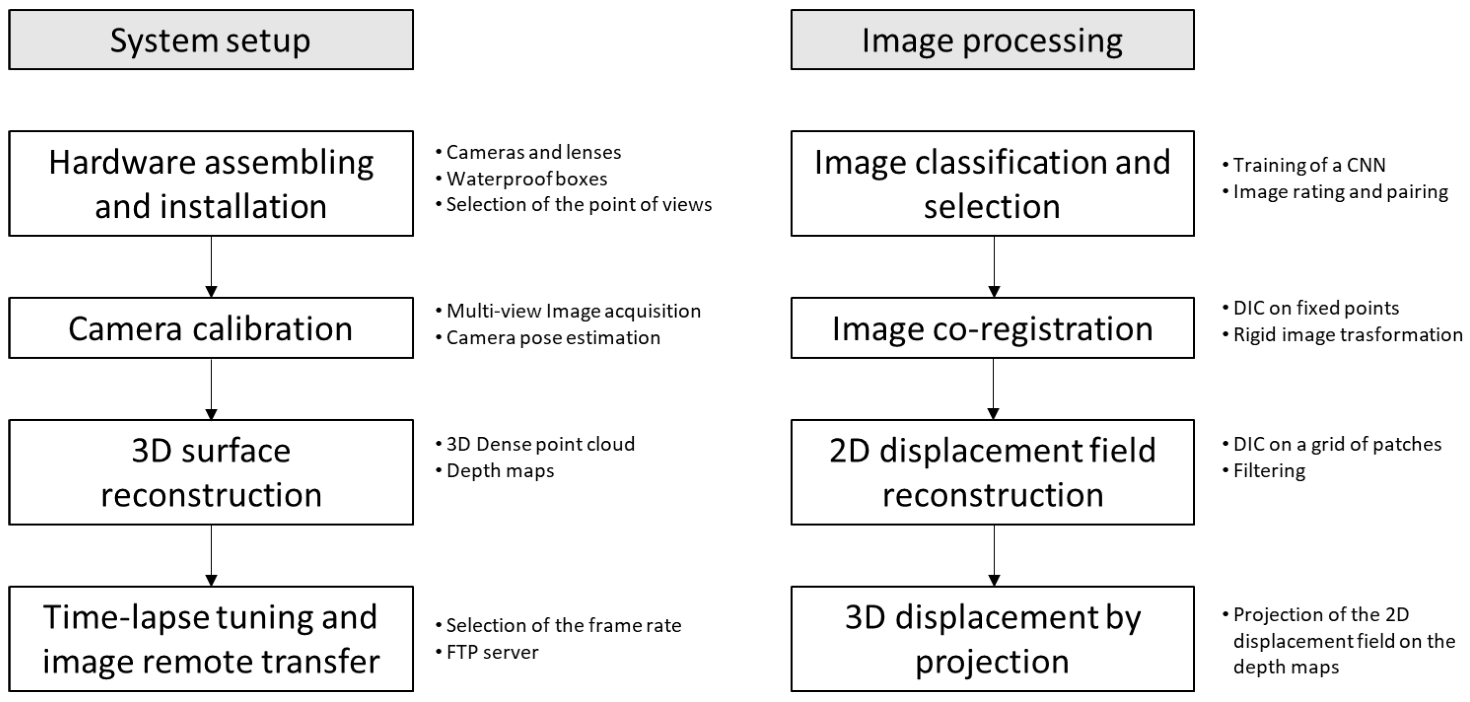
2. Methods and Instrument

The conceptual framework of the proposed methodology is illustrated in Figure 1. Differently from other techniques, the DIPHORM (DIgital PHOtogrammetRic Monitoring) technique distinguishes itself by involving a sequence of several operations that can be divided into two main phases that must be carried out in sequence, as shown in Figure 1. The first phase consists of all the preparatory steps necessary for setting up the system, which are listed on the left side of Figure 1. These steps include assembling and installing the hardware in the appropriate configuration, calibrating the system, creating a point cloud of the scene, and configuring the time-lapse and the FTP server for image transfer. Camera calibration and surface reconstruction must be conducted during the initial setup and after any significant system maintenance, such as changes in optical settings, camera relocations, or notable alterations to the monitored area.
The second phase, shown on the right side of Figure 1, pertains to the ongoing monitoring activities. These activities include downloading images, evaluating and classifying them, aligning the images, detecting displacements on the image plane, and projecting measurements onto the 3D map of the scene. These operations are carried out continuously, for instance, on a daily basis, for the entire duration of the landslide monitoring period.

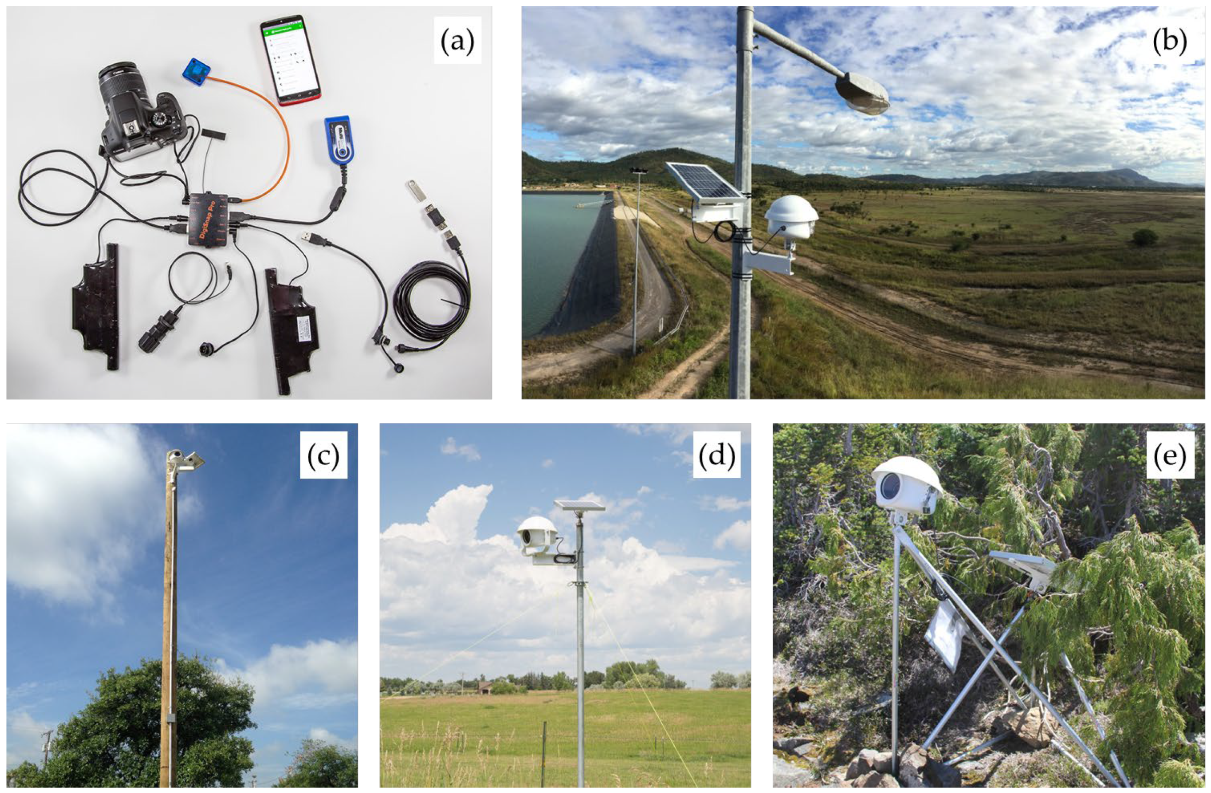
2.1. Hardware Configuration and Calibration

The core of the DIPHORM hardware setup consists of cameras set to capture images with a time frequency adaptable to field conditions. The optional choice to use multiple cameras may be driven by the principle of redundancy, which is fundamental for establishing a reliable monitoring network, especially if it includes warning functions. This strategy ensures the maintenance of the system functionality, even if a main component of the network fails. Redundancy may be extended not only to the image acquisition system but also to the remote storage and transmission, guaranteeing continuous operation despite the loss of any monitoring component.
The selection of cameras and lenses most adapted for this use is based on a balance of resolution requirements, site-specific conditions (e.g., the distance from the landslide and its surficial extension), general photogrammetry guidelines (e.g., optimal camera specifics and positioning), and budget considerations. Typically, wide prime lenses are preferred over ultra-wide or fish-eye lenses, and high-resolution mirrorless cameras with large sensors are ideal for this application [31]. However, it should be noted that the accuracy and precision of DIPHORM can be lower compared to traditional methods such as topographic surveys using theodolites or GNSS receivers. This is primarily due to the reliance on image correlation techniques, which can introduce errors in displacement measurements, especially in complex terrains or when the camera-to-landslide distance is significant, leading to reduced resolution and increased uncertainty in displacement calculations.
For outdoor use, each camera must be mounted in a protective waterproof box and equipped with external hardware to trigger the camera shutter and remotely transmit and upload the images via a network connection (Figure 2a). In addition, a framerate adjustment system adaptable to specific monitoring needs and a local memory enhance the system’s robustness and effectiveness. A solar panel and a battery complete the equipment: they ensure electrical power supply, even without a connection via cable or during service interruption. In this way, the system automation allows minimization of the maintenance activities after its on-site installation (Figure 2b–e).
Before installing fixed cameras on site, and whenever operating conditions significantly change, camera calibration is required. This process aims to determine two groups of camera parameters: intrinsic and extrinsic [32,33]. Without these parameters, the results obtained from image analysis cannot be accurately projected into the calibrated three-dimensional space. Intrinsic parameters refer to the physical and technical characteristics of each camera, such as the pixel size, the focal length, the misalignment of the optical axis, and the optical radial and tangential distortion parameters, which are necessary for referencing the geometrical configuration of an ideal pinhole camera. Extrinsic parameters contain information about the on-site geometrical configuration of cameras, specifically their positions and orientations relative to a world reference system.
The calibration process is critical for ensuring precise measurements, but it can be highly dependent on the specific site. Variations in camera setups, environmental conditions, and characteristics of the monitored area can result in different calibration outcomes, potentially requiring frequent recalibrations. This can be time-consuming and resource-intensive. Moreover, the accuracy of the calibration largely depends on the quality and distribution of Ground Control Points (GCPs). Poorly distributed or low-quality GCPs can lead to inadequate calibration, resulting in errors in 3D reconstruction and displacement measurements. Accurate estimation of camera parameters is critical for the accuracy of displacement measurements in the following stages. It should be noted that the standard laboratory calibration with a chessboard that generally provides good overall accuracy is unsuitable for this application where the distances between cameras and the subject are within the limit of close-range photogrammetry [34,35,36].
For this outdoor application, with calibration involving multiple cameras, multiple poses, and fixed rigs, two strategies have been identified, both adopting the well-known Structure-from-Motion (SfM) and Multi-View Stereopsis (MVS) workflows [32,33,37]. The two strategies consist of the following, and can be used alternatively: (a) directly obtain an unreferenced point cloud of the scene and then scale, rotate, and translate this point cloud using a distance minimization strategy like Iterative Closest Point (ICP) to match a previously obtained reference point cloud [38]; (b) identify some reference points in multiple views whose coordinates are known and use their positions as constraints in the SfM-MVS workflow. Both methods have been tested using Agisoft Metashape (v. 2.0.1, Agisoft LLC, 64 Kirochnaya street, St. Petersburg, Russia, 191015) for intrinsic and extrinsic calibration, Cloud Compare (v.2.11, CloudCompare, www.cloudcompare.com) for ICP co-registration, and MATLAB (R2021a, MathWorks) for data processing. Both strategies have shown good results, although the comparison between the two may be site dependent.
Photo acquisition should preferably be performed using the same cameras intended for the time-lapse monitoring from the fixed locations. Initially, photos of the landslide are taken from various “free” positions, ensuring at least 40 convergent photos from different points of view with 70–80% overlap of the scene. The final photos are taken after mounting the cameras in the fixed boxes and their poses, which are estimated during the camera calibration, will be used in the subsequent phases (Figure 3a).
Other general guidelines for the camera settings and operations during the outdoor calibration phase include the following: (i) prioritizing aperture over shutter speed; (ii) keeping ISO settings as low as possible; (iii) disabling the auto-focus; and (iv) preferring cloudy days to avoid shadow cast. Taking multiple photos from the same fixed position can also improve the accuracy of the calibration and the 3D reconstruction [19]. Once photos are acquired, the feature detection, key points matching, and bundle adjustment processes allow one to build the point cloud and determine the camera parameters (Figure 3b).
For camera calibration and georeferencing (both using methodology (a) or (b)), high-contrast and easily recognizable objects should be used as reference targets, namely Ground Control Points (GCPs). Suitable GCPs include edges and corners of rocks or buildings, as well as specially designed fixed objects like spheres and optical targets. The coordinates of GCPs must be acquired through GNSS surveys to ensure high spatial accuracy and precision. Their position can be also subsequently updated with the use of a total station if future updates to the scene are needed, avoiding the need to revisit the landslide area after the initial calibration.
The calibration process determines the camera poses (positions and orientations, i.e., the external parameters) and the camera internal parameters, which are subsequently used in the Multi-View Stereopsis (MVS) phase to generate a georeferenced 3D dense point cloud of the landslide surface. This 3D surface represents the reference used in the subsequent tasks for transforming the 2D displacements determined on the image planes into accurately scaled 3D vectors (Figure 3c). Alternatively, the projection surface can be obtained from a ground- or air-based laser scanner survey [39], but the cameras must still be calibrated (internally and externally) on this surface [39]. If the 3D reference surface is obtained with a laser scanner, the camera positions and orientations must be back-calculated by co-registering the point clouds and/or the images with some GCPs. The choice of reference surface depends on user availability, site characteristics, and the desired measurement resolution [40].
After collecting images for the calibration phase and fixing the cameras in their boxes, the cameras must be set to fully automatic mode for both shooting and sending photos to an FTP server (Figure 3d). The time step for the image acquisition can be adjusted based on the expected displacement rate of the landslide and the need for near real-time monitoring (Figure 3e,f).

2.2. Time-Lapse Image Processing

After completing the installation and camera calibration phases, the monitoring process begins with the time-lapse image processing. All the subsequent steps have been specifically coded and executed in the MATLAB environment.
Firstly, photos are downloaded from the FTP server and pre-processed in order to select only the best images for the following digital image correlation process. For this purpose, this selection is carried out using a GoogLeNet Convolutional Neural Network [41,42] trained on 2750 images labeled with their corresponding class rate. The photos of the landslide are resized to 224 × 224 pixels and classified on a quality scale from 1 to 5 as follows:
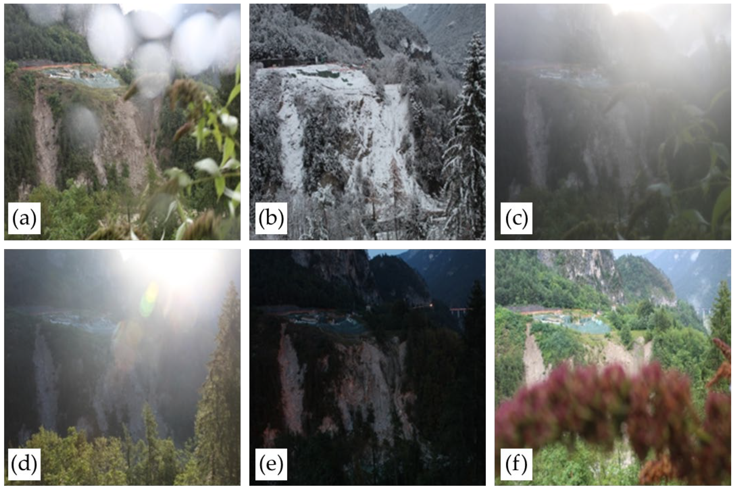
  • Very low (rate 1): images with evident disturbances, making them unusable. The neural network was also trained to identify the reason for the disturbance, such as the presence of rain, snow, fog, glare, darkness, or other elements (Figure 4a–f);
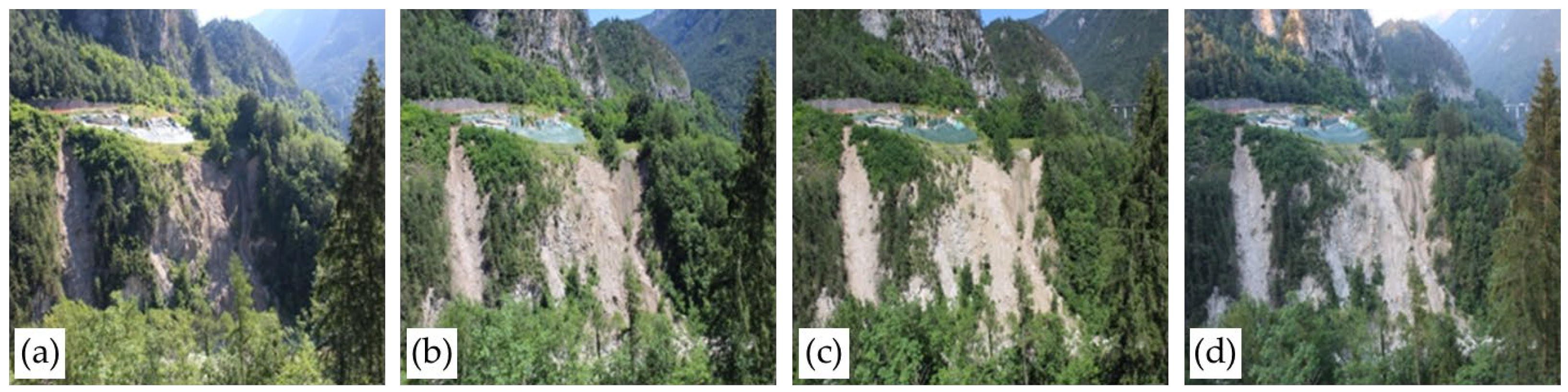
  • Medium (rates 2 and 3): photos with shadow casts that reduce the overall quality but are still usable (Figure 5a,b);
  • Good and very good (rates 4 and 5): high-quality images (Figure 5c,d).
If multiple images have the same score on a given day, the image taken at the same or at the closest time to the previous day’s photo is selected when possible.
The second step of the pre-processing phase involves image undistortion. An algorithm maps the pixel locations of the output undistorted image to the input original image using a reverse mapping technique. The correction of the camera lens distortion is based on the intrinsic camera parameters obtained during the calibration phase.
The third pre-processing step addresses the correction of minor rigid displacements of the camera view due to slight box oscillations, which can create artifacts in the reconstructed displacement field, amplified by the long distance from the slope. It is indeed possible that wind, the passage of heavy objects near the cameras, or other external factors may cause oscillations in the supports of the monitoring systems. To correct these unwanted movements like small oscillations around a position considered neutral, a fine-tuning digital correlation algorithm is used, followed by applying a rigid transformation to the rectified images. For this purpose, some reference elements, such as building corners or high-contrast structures in the stable portion of the slope, can be used as anchors for these adjustments. However, if the camera displacements are more significant or if they tend to accumulate in the same direction, it may be necessary to recalibrate the system in its new configuration.
After the pre-processing, the images are analyzed in pairs using a digital image correlation (DIC) technique applied to an area of interest of the scene in the time-lapse sequence. Among the DIC algorithms, the authors selected the normalized cross-correlation metric, widely used in particle velocimetry analyses [24,26,43]. This method proved to be robust for analyzing textured surfaces of materials such as soils and rocks. The patch size used for tracking displacement can be adjusted based on the image characteristics, camera specifications, the scene–camera distance, and the local shape of the monitored slope. A Eulerian is preferred over a Lagrangian approach, keeping the grid of patches fixed in the image, and facilitating straightforward filtering and interpolation.
The DIC technique reconstructs the 2D displacement field of the scene in pixels, based on a temporal basis given by the shooting times of the selected photos (Figure 3e). This allows for an initial qualitative evaluation of the movement distribution, roughly identifying areas with a significant displacement rate and stable regions. However, for precise quantification of movements, the 2D displacement field of each camera must be projected on the 3D scene (Figure 3f). This projection is performed by using the depth map of each camera, derived from the 3D point cloud of the slope surface and the extrinsic and intrinsic parameters of each calibrated camera. Each camera view has a unique depth map that provides, for each pixel on the image, the object-to-camera distance and the local orientation of the slope surface. Local spatial interpolation strategies must be applied to reconstruct a smooth, speckle-free depth map, depending on the quality and the point density of the original 3D point cloud and the eventual presence of occlusions. When the depth value is available for each pixel, a linear interpolation can be applied to the x, y, and z coordinates of each starting and final point of the displacement vectors.
Depth maps also allow us to estimate, for each image pixel, the ground sample distance (GSD), also known as ground pixel size (expressed in m/px), directly related to the local spatial accuracy. Generally, points closer to the camera have a smaller GSD value and higher displacement evaluation accuracy. However, for non-nadiral images such as terrestrial photos, the angle θ between the normal vector to the slope surface in a given point and the line of sight along the camera-point direction (Figure 6 and Table 1) significantly affects the final GSD value [44]. The distribution of GSD values and θ angles of the scene may help to identify and distinguish areas with potentially accurate monitoring results and regions where displacement measurements may be less reliable. For instance, high θ values (>70–80°) combined with large distances result in high GSD and low-resolution displacement values. Photogrammetric monitoring is indeed very effective at detecting displacements perpendicular to the image plane but less efficient at measuring displacements along the line of sight. The angle θ thus allows for expressing the reliability of the method based on the "visibility" of the terrain potentially subject to displacements.
Another crucial aspect is collecting images at time intervals (time step) to ensure the consistency of the analyzed sequence. In other words, two successive images should be similar enough to allow an effective patch matching in both photos, even if slightly moved or deformed. An evaluation of the matching degree characterizing each element in subsequent images can be quantified in image processing using the estimation of the normalized cross-correlation value. In outdoor applications, it should be noted that shadows produced by clouds or by relevant slope irregularities may degrade the final results and, consequently, an image with diffuse light is preferable. Similarly, daily images taken at the same time help to reduce the effect of movement artifacts induced by shadow casts.
Determining a single general rule for the optimal temporal monitoring resolution can be challenging due to several factors, including the landslide displacement rate and trend over time, the impact of surface erosion, and the visibility conditions of the slope. For instance, monitoring a rapidly moving landslide might require a time resolution of several images per hour, whereas a slow-moving one might only need one photo per day. High erosion susceptibility and poor visibility conditions (e.g., recurrent fog) typically necessitate an increased acquisition frequency to obtain a sufficient number of usable images.

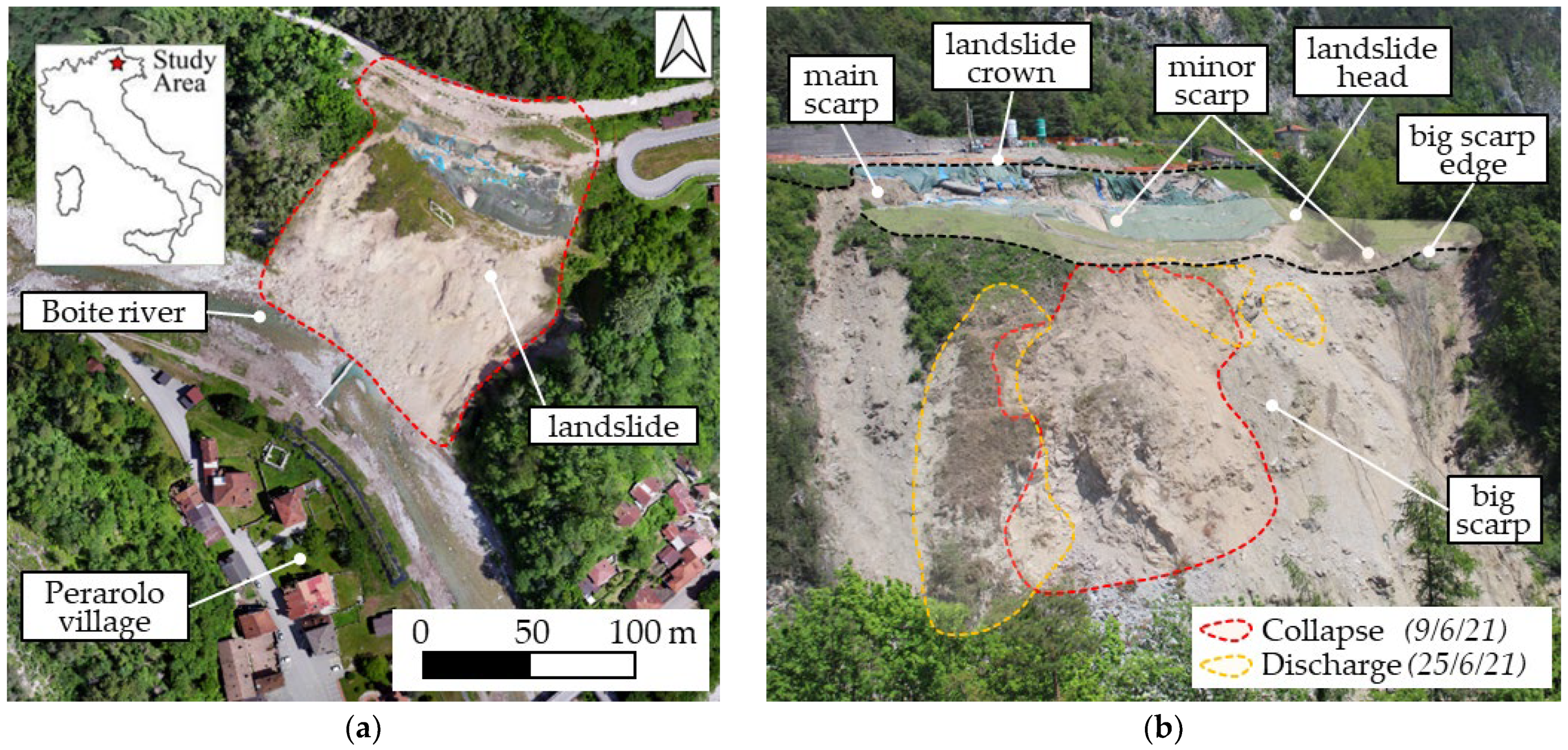
3. The Sant’Andrea Landslide

3.1. Site Description

The Sant’Andrea landslide is located in the municipality of Perarolo di Cadore, in the Province of Belluno (northeastern Alps, Italy). This mass movement affects the left flank of the Boite River, posing a significant hydrogeological hazard to the village downstream (Figure 7a). The currently unstable area is part of a larger, older slope deformation involving the southern slope of Mt. Zucco, the main peak in the area. Although instability signs have been present in the unstable area since the late 20th century, the Sant’Andrea landslide has become more active in recent years, with a progressive worsening of the instability conditions and an enlargement of the mobilized area. Attempts to stabilize the slope in the 1980s and 1990s provided only temporary effects, as movements gradually reactivated. The interventions carried out at the Sant’Andrea landslide include retaining walls, micropiles, and stormwater drainage systems [28].
The landslide kinematics are characterized by alternating slow displacements and acceleration phases, with the latter being triggered by both heavy and prolonged rainfall events [28,29,30]. In 2021, the landslide experienced a long phase of progressive acceleration, with significant displacements primarily affecting the central part. Moreover, following a long rainy spring, in the first week of June, a sudden collapse of around 8000 m3 from the central front (Figure 7b) occurred. In order to increase safety in the area, the collapse of two smaller portions of the frontal area (Figure 7b), for a total volume of about 3000 m3, was induced with explosives at the end of June.
Several investigations, including boreholes and geophysical surveys, were conducted in different stages between 1997 and 2019 [28]. These revealed that the landslide primarily involves a 30 m thick layer of calcareous debris located above an evaporitic-rich bedrock. The debris deposit consists of a chaotic mix of rock fragments (boulders, gravel, and sand) in a silt and clay matrix with a highly heterogeneous grain-size composition. The bedrock is composed of a marly limestone lithology, known locally as the Travenanzes formation, characterized by highly stratified and alterable anhydrite–gypsum layers, strongly deformed and folded by the Alpine orogeny. The fractured upper part of the bedrock seems to control the landslide dynamic, although the sliding surface is not uniquely confined in a specific layer or at the debris–bedrock interface. A complex hydrogeological framework of the area is driven by the spatial and in-depth variability in the lithological units. Within the moving mass, two groundwater systems were identified [28]: a shallow water circulation flows through the debris layer, whereas a deeper one in the weak gypsum layer forms the upper part of the Travenanzes unit.
The groundwater coming from the upstream zone, as well as the meteoric water infiltrating the landslide area, induces hydration and dissolution processes within the weak gypsum layers. Gypsum alteration causes the formation of microcracks that expand with active water circulation, creating voids that weaken the mechanical properties of the bedrock. This process leads to the development of plastic rheology [45,46], which is considered the primary factor in the creep displacements of the slope. For these reasons, the kinematic mechanism of the Sant’Andrea landslide is a combination of long-term creep deformation related to the geological properties of gypsum layers and rain-induced acceleration phases.

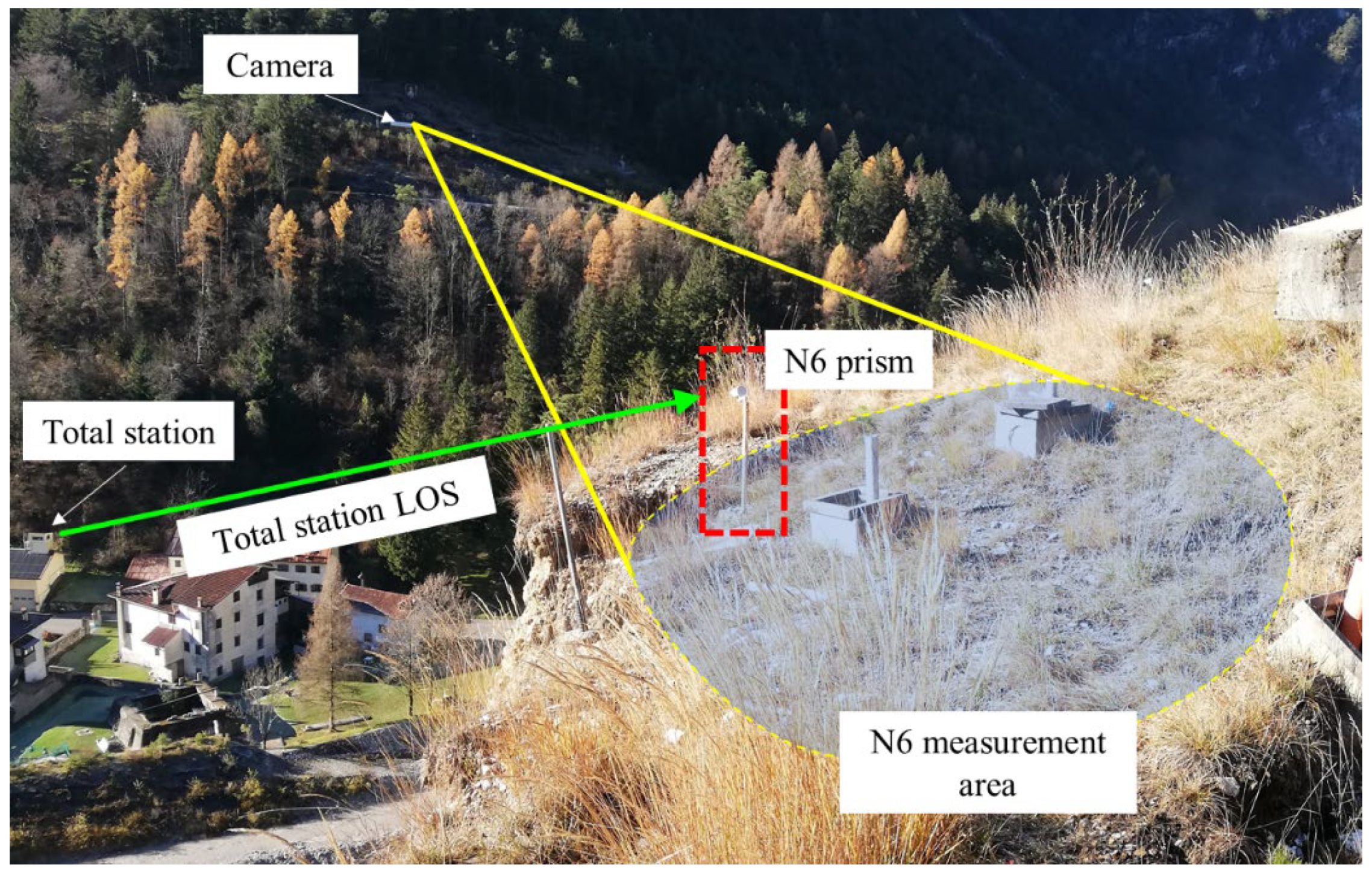
3.2. Monitoring System

Although the first evidence of movements dates back to 1986, comprehensive monitoring of the landslide began only in the early 2000s with the installation of some extensometers, a GPS receiver, and two inclinometers. Unfortunately, the inclinometers became non-functional for excessive distortions and no further inclinometers were installed. Since 2013, a topographic system has been implemented for the monitoring of surficial slope displacements. It consists of a Leica robotic total station (RTS) that records the position of a finite set of optical targets (approximately 30) installed in accessible zones of the landslide site, i.e., above the bottom black dashed line reported in Figure 7b. Over the years, the number of targets on the unstable slope has been increased to enhance the spatial assessment of displacements (Table 2). However, targets placed on the big scarp or close to its edge were frequently lost due to erosion and small collapses occurring in very steep areas of the slope.
The monitoring revealed that the landslide exhibits intermittent activity, which is characterized by evident periods of acceleration and slowdowns. Traditionally, a scattered displacement field has been observed, with portions of the slope that become temporally unstable and then apparently stabilizing. Nevertheless, the kinematics and the extent of these unstable portions were difficult to recognize, necessitating an overview of the entire slope.
Based on the landslide displacements assessment, RTS data indicate a progressive worsening of slope stability, with an enlargement of areas experiencing larger displacements, particularly in the period from 2019 to 2021, and a consistently high mean acceleration over the long term. This evolution is evident in the annual total displacements (Table 2) and the trend of cumulative displacements (Figure 8) of some targets on the slope. The selected targets can be grouped based on their kinematic behavior: GPS1, N6, P3, P28, P24, C1, P4, P8, P13, and P19 show high displacements, while N3, P1, and N10 are stable. Note that P28 and P24 were installed only in May 2016, while N10, GPS1, and N6 were installed in July 2018 and C1 in December 2020. Some targets, such as N6 and P3, were non-functional for over two years (from February 2019 to March 2021) and returned to operation only after system maintenance. Due to worsening slope conditions, five additional targets (PR1-PR5) were installed in April 2021 to track the slope portions close to the big scarp showing significant signs of mobility. However, PR1 and PR2 lasted only 64 days before being destroyed in the major collapse on 9 June 2021.
In general, the mean daily displacement rate in the unstable area was less than 1 mm/day from 2014 to 2018, increased to 2 mm/day in 2019–2020, and dramatically reached 20 mm/day between late 2020 and early 2021. PR1 and PR2 measured more than half a meter of deformation in about two months, with a marked deterioration in late May and early June. Following the natural and explosive-induced collapses of June 2021, the displacement rate decreased to 4 mm/day, indicating a move towards a more stable condition. Consequently, the total displacement significantly decreased in 2022 compared to the previous year (Table 2).
Although the availability of RTS data has significantly increased the understanding of landslide dynamics, this monitoring system has notable disadvantages that are evident in this application. Firstly, it is impossible to infer any information about the displacement rate of the main scarp, where no targets are available. Consequently, identifying which portions of the steep scarp are involved in the instability is not feasible. Secondly, continuous and repeated maintenance work, including the installation of new targets, is required. This aspect, in addition to a high monetary cost, necessitates access to potentially unstable areas of the landslide, an activity that is potentially very dangerous for the personnel involved.
The punctual topographic information can be spatially interpolated using the Inverse Distance Weighting (IDW) method in the QGIS environment. Figure 9a,b illustrate maps of the total displacements cumulated in the period April–May 2021 and August–September 2021, respectively. Horizontal displacements are also shown on the maps as arrows starting from each target position. It is immediately notable how interpolation results strongly depend on target availability. For instance, in Figure 9a, the displacement contour covers a larger area, extending inside the main scarp. However, in the post-collapse condition, the landslide portion in which displacement information can be obtained is significantly reduced (Figure 9b). Furthermore, no information can be obtained in the big scarp, below its main edge. The comparison between the two maps reveals that the displacement magnitude in the central portion decreased after the collapse, indicating the lightened slope has reached a new temporary condition of equilibrium.

3.3. Photogrammetric Monitoring

In order to overcome the limitations of the topographic survey mentioned in the previous section, a new photogrammetric monitoring was installed in 2021. This system consists of three Canon EOS 1300D cameras (Canon, Tokyo, Japan), each equipped with a Canon EF-S 18–55 mm f/3.5–5.6 IS STM lens. The use of three cameras, as anticipated, ensures system redundancy, allowing continuous image acquisition over time even if one unit stops working. During the period considered for this work, all cameras were operational, enabling measurements using the images coming from a single camera. The cameras were installed on the opposite side of the Boite Valley, directly in front of the unstable area, at a distance of approximately 350 m, as shown in Figure 10a. Each camera is mounted inside a waterproof box connected to a steel pile (Figure 10b,c) and equipped with a DigiSnap Pro controller for time-lapse control, a modem for internet connectivity, a USB flash drive for local storage, a 92 Wh battery, and a 20 W solar panel. Following a calibration and testing period, the system has been completely operational since May 2021.
The calibration was carried out by processing about 50–60 photos per camera taken from the fixed positions and several other standpoints. The procedure allowed the identification of the intrinsic and extrinsic parameters of each camera and the creation of a photogrammetric point cloud of the landslide site. GPS coordinates of some edges and corners of existing structures in the area and four manually placed spherical targets (Figure 10d,e) were used to georeference the point cloud. At the same time, a laser scanning survey was performed (Figure 10f), providing a further accurate and detailed 3D reconstruction of the area. Considering the landslide displacement rates derived from RTS measurements and the potential for poor visibility images, it was decided to capture one image every 30 min.
The photo pre-processing, as described in Section 2.2, was applied to the image sequence acquired from May 2021 to September 2022 (almost 10,000 pictures) with a two-step Convolutional Neural Network procedure. In the first phase, unusable photos (rate = 1) were identified (25% of the total) and classified based on the presence of fog (14%), snow (5%), rain (1%), or other strong disturbing elements on the scene, such as darkness (4%) or sun glare (1%). In the second phase, the remaining images were evaluated based on quality, with the best light conditions receiving a maximum rate of 5 (27% of the total), and usable but lower-quality images receiving a minimum rate of 2 (34% of the total). Finally, to compose a sequence of daily images for the following displacement analysis, one image with the highest rate was chosen for each day, prioritizing the shooting time of the previous day. If no sufficiently high-quality image was available for certain days, the time sequence was reconstructed with the next suitable image to maintain the temporal continuity of the monitoring.
As mentioned in Section 2.2, selected images were aligned to reduce small shifts caused by the vibration of the camera support. To this aim, some stable reference points were identified at the border of the concrete wall on the rear of the landslide and at the corners of external buildings (Figure 3b). The alignment of the images was then achieved using a rigid transformation based on the results of a cross-correlation algorithm applied to the positions of the reference points. For the digital correlation analysis of the daily image sequence, a fixed regular grid of square patches (40 pixels per side and spacing) was applied, covering the landslide area only. Background and foreground objects, as well as trees, were masked. The Eulerian displacement field of the points of the grid on the 2D image plane was obtained using a normal cross-correlation algorithm with a minimum threshold value of 0.70. This value also helps to discard points on ridges or edges of the landslide surface where, in the same patches, pixels may have significantly different distances or orientations from the normal vectors. A second filter discarded displacement values with pixel modulus scores greater than the 99th percentile.
The 3D projection of the 2D displacements was carried out using the laser scanner point cloud of the landslide. Firstly, the point cloud was first roto-translated to match the camera reference system and then used to construct the mesh of the surface. Linear interpolation was employed to obtain the metric coordinates in the world reference system for each pixel forming every image of the time sequence, excluding occlusions (depth map). The 2D displacement vectors for each patch were then projected to obtain the initial and final points of the 3D displacement vectors.
In the data projection from 2D to 3D, a third filter excludes the measurements based on the local θ angle (Figure 11a), i.e., the angle between the normal vector to the slope surface in that point and the line of sight along the camera-point direction, as described in Section 2.2. Figure 11b shows a map of the local ground sample distance (GSD) calculated according to [44], considering the effect of the local θ angle. This map allows us to identify areas where monitoring results are highly reliable and areas where the obtained displacements may be less accurate. In our case, a threshold of 70° was adopted: points with a local θ angle greater than 70° were discarded.
Temporal interpolation was then performed to fill any portions where measurements were missing due to the first and second filters (caused by a lack of high-quality images during some periods). However, data discarded by the third filter were not interpolated.
To ensure the accurate projection of 2D measurements onto a 3D slope map, a new laser scanner cloud was acquired after each collapse or significant variation in the shape of the slope, resulting in an update of the 3D map of the scene. In total, the depth map onto which the data are projected has been updated five times: on 11 June after the natural collapse, on 25 June following the artificial collapse induced by explosives, and on 7 September 2021; in addition, the depth map was updated on 25 March and 19 July 2022 during inspections for maintenance operations.

4. Results

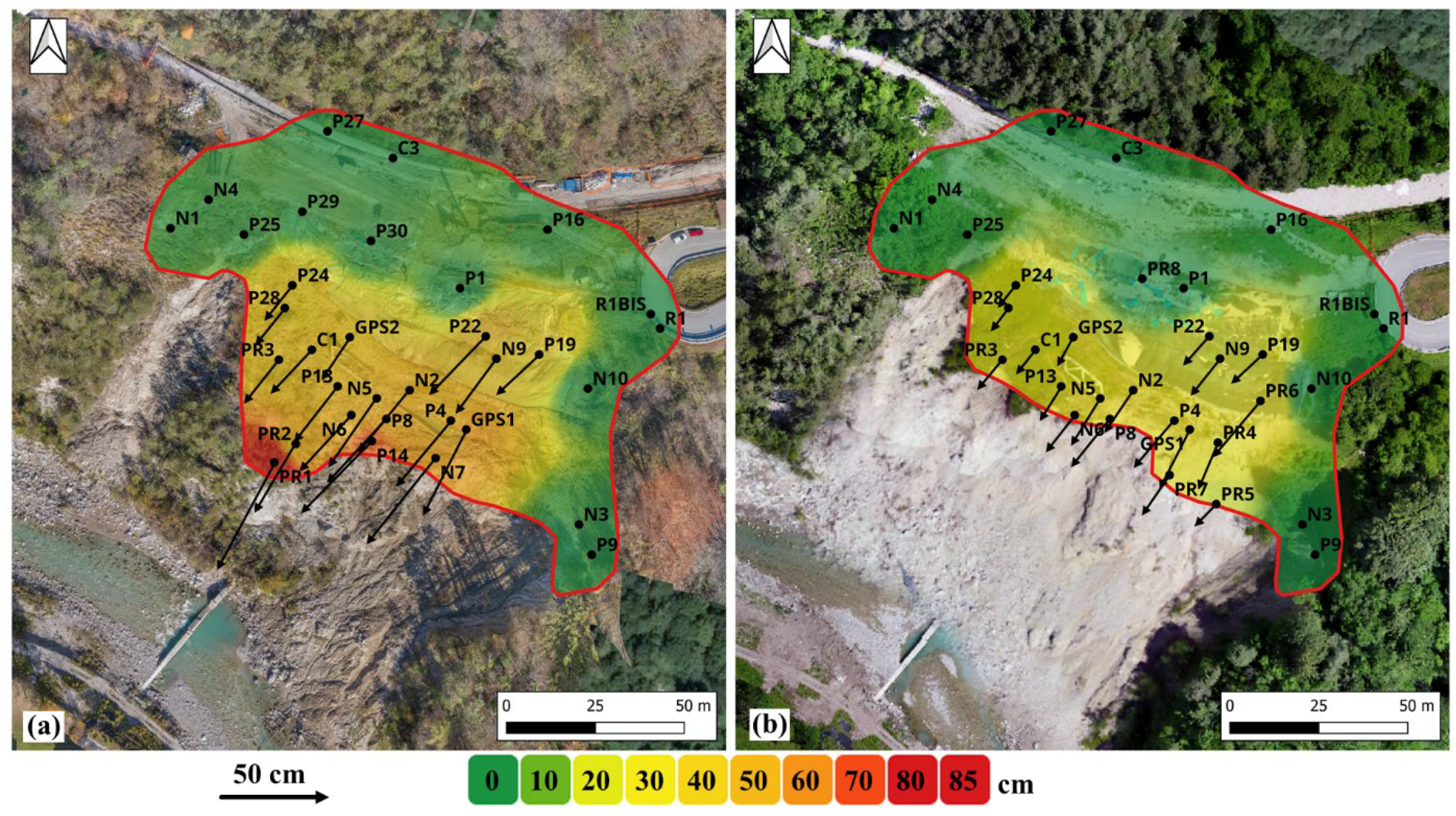
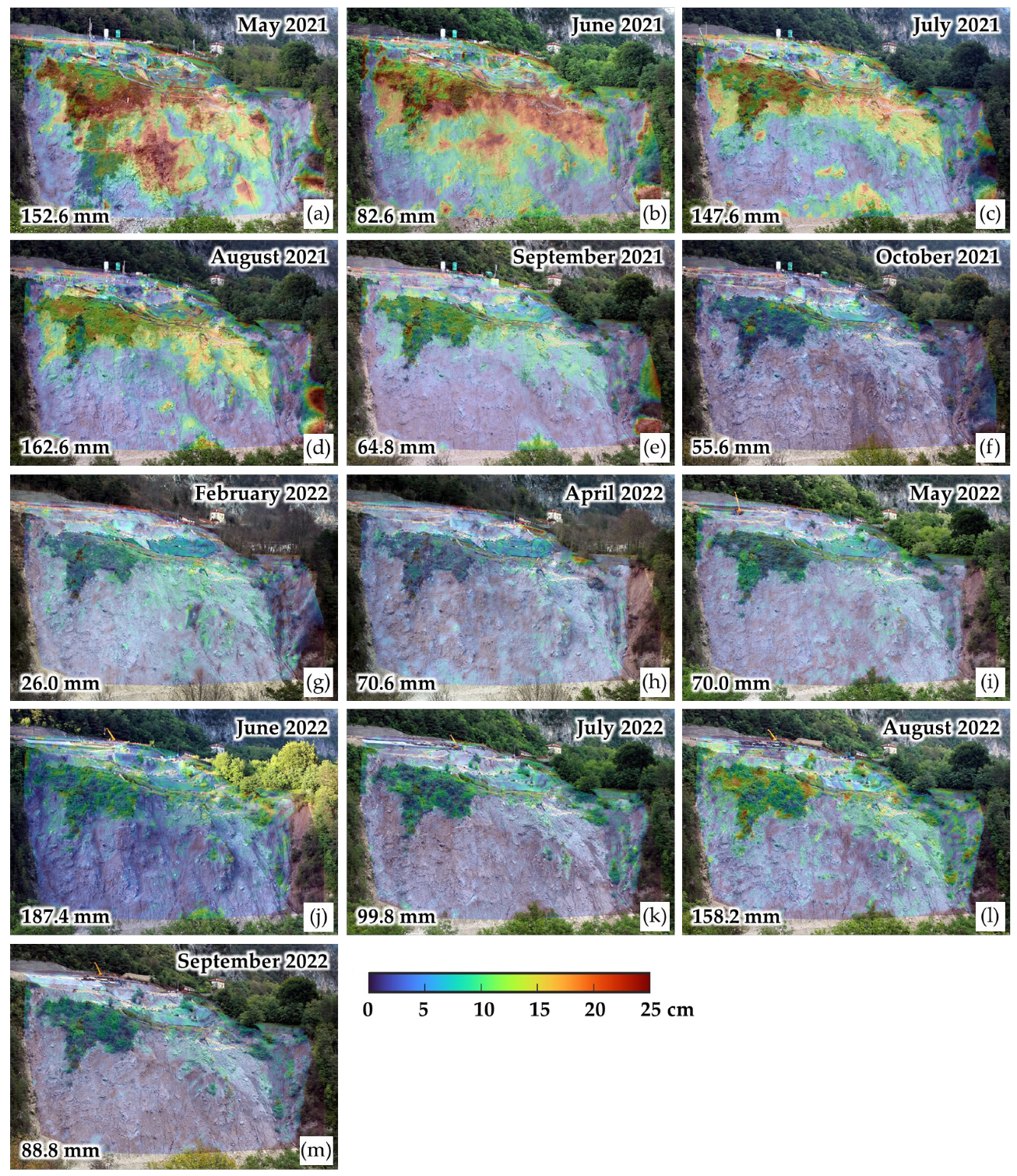
4.1. Cumulative Displacement Maps

The results of the DIPHORM method can be effectively visualized in the form of cumulative displacement maps. For instance, the contour maps in Figure 12 represent the distribution of the monthly displacement obtained by the photogrammetric monitoring system, superimposed on the photo taken on the last day of each reference month. However, the analysis is missing data for November and December 2021, as well as January and March 2022, due to a lack of good-quality images caused by snow, rain, or fog. Consequently, monitoring data for these months are not available. Nevertheless, the monitoring system returns immediately operational as soon as a photo of adequate quality is obtained.
From May to July 2021 (Figure 12a–c), significant movements exceeding 25 cm/month were observed, while a marked reduction in instability was evidenced in the following months. In May (Figure 12a), displacements were concentrated in the central part of the big scarp, particularly at a rocky ridge. The collapse on 9 June lightened this portion by a volume of approximately 8000 m3, resulting in a significant decrease in the displacement magnitude in that area. The second collapse on 25 June, artificially induced, involved a volume of around 3000 m3, containing the remaining vegetated portion on the left (compare Figure 12a,b), and produced a further reduction in the deformation trend. In June 2021, movements were still fairly distributed over the upper area, but the lightening of the slope allowed it to achieve a more stable condition in the portion of the big scarp. In July and August 2021 (Figure 12c,d), the displacement maps show persistent deformation in the upper part of the slope, probably related to a slower equilibrium resetting. Observing the monthly series from May to October 2021 (Figure 12a–f), it is clear that the slope evolved its kinematics over time, reaching an almost “stable” condition with constant velocity by October.
Figure 12 also highlights the intermittent nature of movements, not always linked to rainfall. February 2022 (Figure 12g) is characterized by higher displacements than April (Figure 12h), likely due to the melting of a thick snowpack accumulated in winter. In April and May 2022 (Figure 12h,i), movements were reduced, while June and August 2022 (Figure 12j–l) showed a slight increase in instability, probably related to intense summer rainfall. Finally, the comparison between May and August 2021 (Figure 12a,d) and May and August 2022 (Figure 12i–m) once again underlines the critical condition of the slope in 2021, and its transition to a new state of slow creep in 2022.

4.2. Validation

The measures obtained with DIPHORM can be validated by comparing the data from the RTS topographic survey acquired during the same period (from 21 May 2021 to 28 September 2022). For this validation, 14 targets were selected (Figure 13) and, for each of them, the average displacement value within a Region of Interest (ROI) surrounding their position was extracted over time. The resultant displacements were used for validation considering that the movements of the monitored points occur almost all in the same direction (see Figure 9 for the top view) and at an inclination of 43° to the vertical.
Targets N3, P1, and N10 (highlighted in green) are representatives of slope areas exhibiting minimal mobility, while the remaining topographic targets are located in active portions of the landslide. Figure 13 also evidences the absence of reflectors below the big scarp edge, with the exception of targets PR1 and PR2 (highlighted in blue). As previously mentioned, topographic monitoring at these locations was only available until the collapse on 9 June 2021, which resulted in their destruction.
Figure 14 compares the displacements of each target monitored by the total station (in blue) and the ones obtained by image analysis (in red) in the period from May 2021 to September 2022. As previously mentioned, three targets (N3, P1, and N10) remained practically immobile for the entire period, with displacements of less than a few millimeters. Figure 14a-c illustrate the displacement trends compared to the measurements obtained with the DIPHORM method. While the displacement rates are nearly negligible, the photogrammetric method reports gentle oscillations up to 40 cm. It is important to note that the cumulative displacement can decrease in this case since it refers to the magnitude of the vector while it cannot become negative.
Topographic data for targets PR1 and PR2, located in the area affected by the first collapse in June, are considered only in the period from 21 May 2021 to 8 June 2021, i.e., before the collapse (Figure 14d,e). The displacement rate determined for these targets confirms the good correspondence between topographic and photogrammetric surveys and also highlights the advantages of photogrammetric surveys. In fact, in these positions, the total station could no longer provide data for PR1 and PR2 as they did not survive the collapse in June, while the photogrammetric system continued its monitoring activity.
From June to the end of September 2021, all other RTS targets indicated a persistence of unstable conditions (Figure 14f–n). In this period, the monthly displacement increment was in the order of 20–30 cm/month (7–9 mm/day) for the targets in the most unstable area, as confirmed by both the photogrammetric and RTS measurements. This displacement rate decreased to 5–6 mm/day by the end of September. It is also interesting to note how the points closest to the area that collapsed in June showed an immediate change in velocity post-collapse.
The areas corresponding to the PR1–PR5 and GPS1 targets showed a significant change in displacement trends, in both topographic and photogrammetric measurements. In contrast, upper areas, such as those at P3, C1, P28, and P24 positions, exhibited a delayed response, taking a few months to establish new kinematic conditions.
The photogrammetric technique effectively captured the change in behavior across the different portions of the slope. It provides not only a reliable displacement value comparable to a traditional precise technique such as topographic surveying, but it also enables local analysis of kinematic trends of the different portions of the slope.
Some differences in the movement trend can be observed for the GPS1, N6, and P3 targets, all positioned at the landslide head. This can be attributed to the high θ angle, and therefore to the lower reliability of the projection of the measurements on the depth map of the scene. Additionally, it should be considered how the measurements of the topographic system are obtained punctually at the ends of the rods of the mentioned targets, while the measurements obtained with the DIPHORM method refer to displacements of the surrounding areas, including points located in the background (Figure 15). The slight oscillations seen in photogrammetric results for targets like N10, P28, P24, PR3, and C1 can be explained by the vegetation growth and drying over the months, which can mislead movement interpretations. However, these oscillations do not compromise the overall reliability of photogrammetric monitoring.

5. Discussion

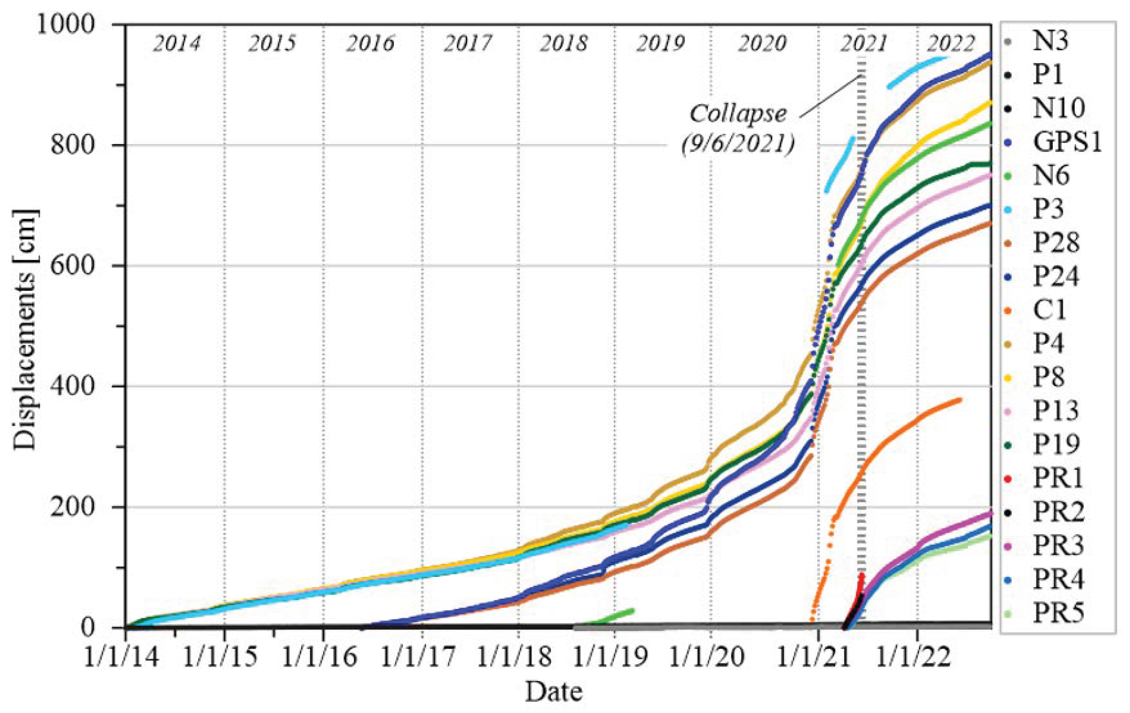
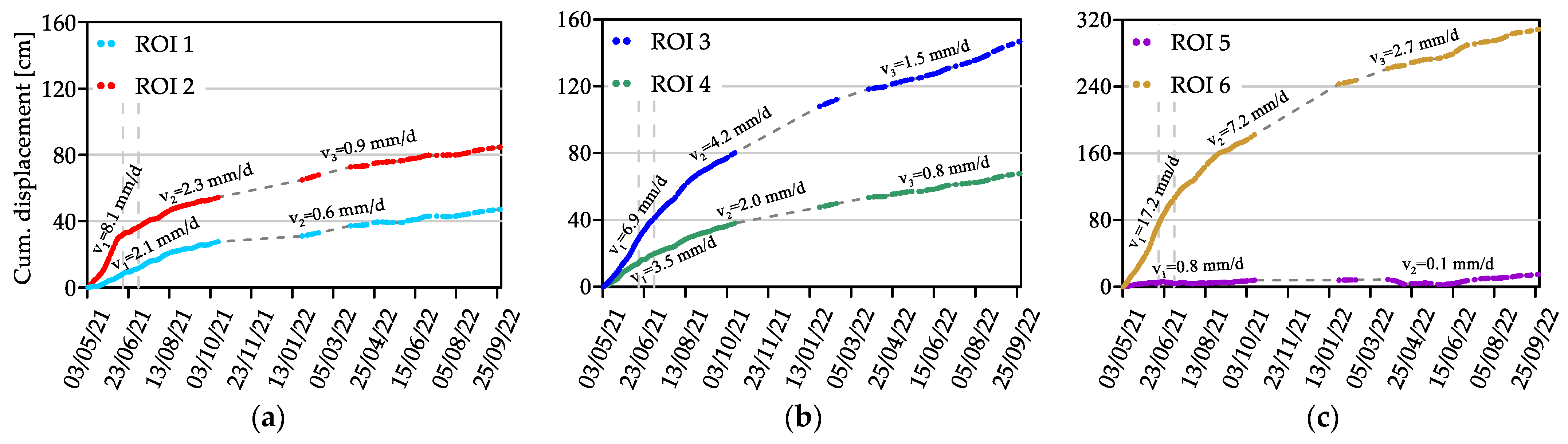
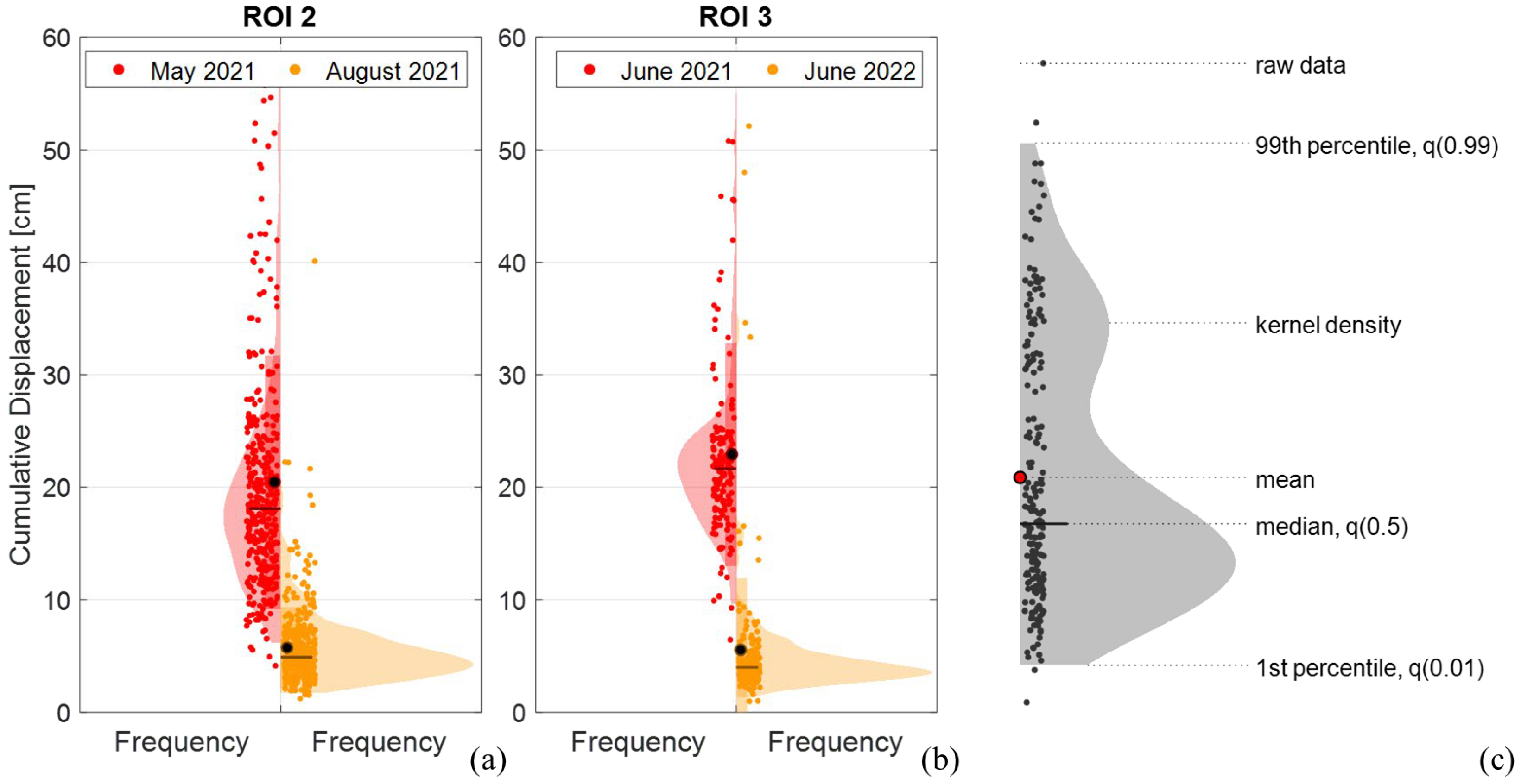
Quantitative Analysis of Displacements

Along with the spatial and temporal analysis of the displacements, the employed method allows further insights into local kinematics within specific Regions of Interest (ROIs). These ROIs can be directly delineated on the image to extrapolate average speeds, average displacement directions, and the distribution of displacements within each region. Therefore, this built software package enables even more detailed visualization of the movements and plots the average movements of each ROI over time, allowing for trend evaluation.
In Figure 16a, six manually selected ROIs on the image are displayed. For each of them, contour maps of the monthly average speed are plotted as well as the average direction of ROI movements, indicated by red arrows. The arrow length is proportional to the total mean displacement cumulated in the month, with the displacement value in millimeters also reported near each vector. This plot can be generated from DIPHORM for any time interval and ROI defined by the user. To better understand the kinematics of the Sant’Andrea landslide, Figure 16 includes data from the period before and after the collapses (May–October 2021, Figure 16a–f) and the period May–July 2022 (Figure 16g–i) for comparison.
Analyzing the movements in May 2021 (Figure 16a), it is easily noticeable that the yellow area in ROI 2 indicates the imminent collapse occurring at the beginning of June 2021. Comparing the contour maps of ROI 2 across different months reveals a generally strong decrease in speed, which then contributes to a gradual accumulation of even smaller displacements. ROIs 3 and 4 also show a trend toward stabilization over the months: May and June 2021 (Figure 16a,b) have similar values, which decrease in July and August (Figure 16c,d), reaching an unchanged state from September onwards.
ROIs 1 and 5, located on the perimeter, generally show limited displacements with values having the same order of magnitude as the method’s sensitivity. Moreover, in these portions and in some periods, the vegetation growth can lead to an erroneous interpretation of the extent and direction of the movements, as already commented. Finally, the upper portion of the landslide (ROI 6), located above the big scarp edge, exhibits the largest movements, particularly from May to August 2021 (Figure 16a–d). However, it is important to note that the projection of the 2D measurements on the 3D map of the scene is critical due to high θ values in many pixels in this area, resulting in lower reliability of the derived 3D displacements. In any case, the displacement analysis remains valid and effectively describes the kinematic evolution of this slope portion over time.
The directions of displacement, represented as arrows at the centroid of the masks, are indicative but may not always accurately reflect the movement patterns. Lastly, while the image offers a comprehensive view of displacement distribution across the slope—very useful for understanding the phenomenon’s evolution over time—it does not ensure high-resolution data for smaller areas. Occasionally, there are isolated pixels of different colors within homogeneous regions, likely due to the imperfect application of DIC techniques to the scene.
Figure 17 shows the trend of cumulative mean displacements of each ROI, along with the velocity characterizing the various periods, derived as a qualitative piecewise linear fitting of the curves. The two collapses in June 2021 are marked by vertical dotted lines. At first glance, all curves show a decrease in their slopes after the two slope lightning events in June 2021, but with different behavior for each region. In particular, the following observations were noted for each of the ROIs:
  • ROI 1: The displacement rate drops from 2.1 mm/d to about one-third of that value starting from September 2021 (Figure 17a);
  • ROI 2: Initially, its displacement rate is very high, at approximately 8.1 mm/d. After the natural collapse, it sharply decreases to 2.3 mm/d and then settles around 1 mm/d in 2022, confirming the strong correlation with the collapses (Figure 17a);
  • ROI 3: Its velocity is maintained around 7 mm/d until August 2021, after which there is a gradual decrease to half the value and a further drop to about 1.5 mm/d from March 2022 (Figure 17b);
  • ROI 4: It shows a gradual decrease in displacement rates, similar to other ROIs, with the final kinematics consistent with the rest of the slope (Figure 17b);
  • ROI 5: It can be considered a control region with very limited displacements for the entire monitoring period. This is aligned with the observations from the topographic targets nearby, which also show almost zero displacements (Figure 17c);
  • ROI 6: It exhibits the highest displacement rates, remaining very high at 17.2 mm/d in the spring and summer of 2021 (Figure 17c). It starts a gradual slow down only from July, halving in the period August–December 2021, and stabilizing at a constant value of 2.7 mm/d starting from 2022.
Although Figure 17 provides important information on the kinematic behavior of selected ROIs, average displacement can be misleading if the region includes portions with very different kinematics. A first evaluation of the reliability of each selected ROI is partially given by the presence of different color gradients within the ROI color maps in Figure 16. However, further investigations can be carried out by considering the displacement distribution within each ROI.
Regarding Figure 17, it can be observed that between October 2021 and January 2022, as well as at the end of February 2022, there are portions of the graph where no data are available due to the lack of usable images during those periods. Although in this specific case, it was possible to mitigate the issue by relying on subsequent measurements that allowed for the interpolation of the missing data—represented in the figure as a dashed line—it is clear that this strategy is not always effective. If the absence of images is excessively prolonged, the reliability of the resulting data becomes questionable, as comparing two images taken at significantly different times may lead to incorrect interpretations.
Figure 18 presents violin plots illustrating the cumulative displacements for ROIs 2 and 3. ROI 2 is chosen because it is representative of the zone where the collapse of June 2021 occurred, while ROI 3 highlights the behavior of another portion of the large scarp of the unstable slope. These plots highlight the statistical distribution of the displacement values across different frequencies. The kernel density immediately identifies the shape of the distribution, while the individual raw measures help understand the data density in each portion of the graph. Fundamental statistics, such as mean and median and 1st and 99th percentiles, are expressed in graphical form, as explained in Figure 18c.
In Figure 18a, the comparison between displacements in May 2021 (in red) and August 2021 (in orange) is related to ROI 2. It reveals a notable shift in the position of the kernel density peak, which was around 18 cm in May 2021 while it dropped to about 5 cm in August. Both distributions present means slightly greater than their medians, underlining that the shape of the distributions is not a perfect Gaussian and that there is a tail towards the high percentiles. The standard deviations of the two distributions also differ: measurements in May 2021 range up to 55 cm, while measurements in August show greater uniformity, clustered near the average. This can be seen from both the shape of the kernel density, the distribution of the raw data, and finally from the amplitude of the 1st and 99th percentiles. This change reflects a significant shift in the kinematics of ROI 2, even if only in a few months, moving from high displacements and variable behavior in May to uniform and reduced speeds in August.
In the same way, Figure 18b compares the measurements of ROI 3 in June 2021 and June 2022, showing a strong decrease in both the displacement value at the peak and the standard deviation. This indicates an overall reduction in displacements and a compaction of distribution towards the average value. The kernel density for June 2022 also shows a minor, secondary peak around 15 cm, potentially suggesting the need to subdivide the region into sub-regions.

6. Conclusions

DIPHORM is a ground-based time-lapse photogrammetric method that enables the provision of a spatially dense evaluation of landslide kinematics, offering information on displacement rates over time and identifying areas with varying instability conditions. This new methodology combines fixed camera internal and external calibration algorithms, surface reconstruction algorithms, and digital image correlation to provide a continuous monitoring tool for the deformation of a landslide slope. The main steps of the DIPHORM method are summarized as follows:
  • System setup: installation, calibration, and tuning of the cameras and of the remote tools, in relation to the phenomenon to be monitored. This permits obtaining the camera pose of the fixed camera and the reference slope surface.
  • Image pre-processing: automatic discarding of the unsuitable images, identification of the optimal images among the remaining ones, and correction of the slight oscillations to which the cameras were subjected.
  • DIC on the image sequence: two-dimensional displacement detection. The 2D vectors are finally projected on the depth map of the scene to obtain a three-dimensional displacement map scaled in metric units.
The method was here validated with reference to the Sant’Andrea landslide. The continuous topographic measurements captured over a dozen RTS optical targets and GNSS receivers installed on the landslide have been compared with the displacement detected by this new photogrammetric monitoring system for 16 months.
The comparison allowed us to identify the following strengths and weaknesses of the photogrammetric system relative to the other conventional topographic methods:
  • Cost efficiency: the equipment for the photogrammetric system is significantly less expensive and can be adjusted to available resources by selecting cameras of varying quality. Traditional techniques, such as topographic or GPS monitoring, are very precise but limited to a few points and require costs of five to ten times higher, including equipment, installation, and management. Multiple surveys using laser scanners require expensive equipment and the presence of an operator, and provide information derived from point cloud differences rather than explicit displacement measurements.
  • Operational flexibility: the monitoring frequency, the selection of areas to be framed, the camera optic, and the image acquisition parameters are entirely site-specific, offering considerable flexibility. On the other hand, RTS and GNSS monitoring require the preliminary choice of the point to be monitored.
  • Spatial density: DIPHORM provides spatially dense and distributed information over the entire framed area, even in locations where target positioning would be difficult, and their stability limited in time.
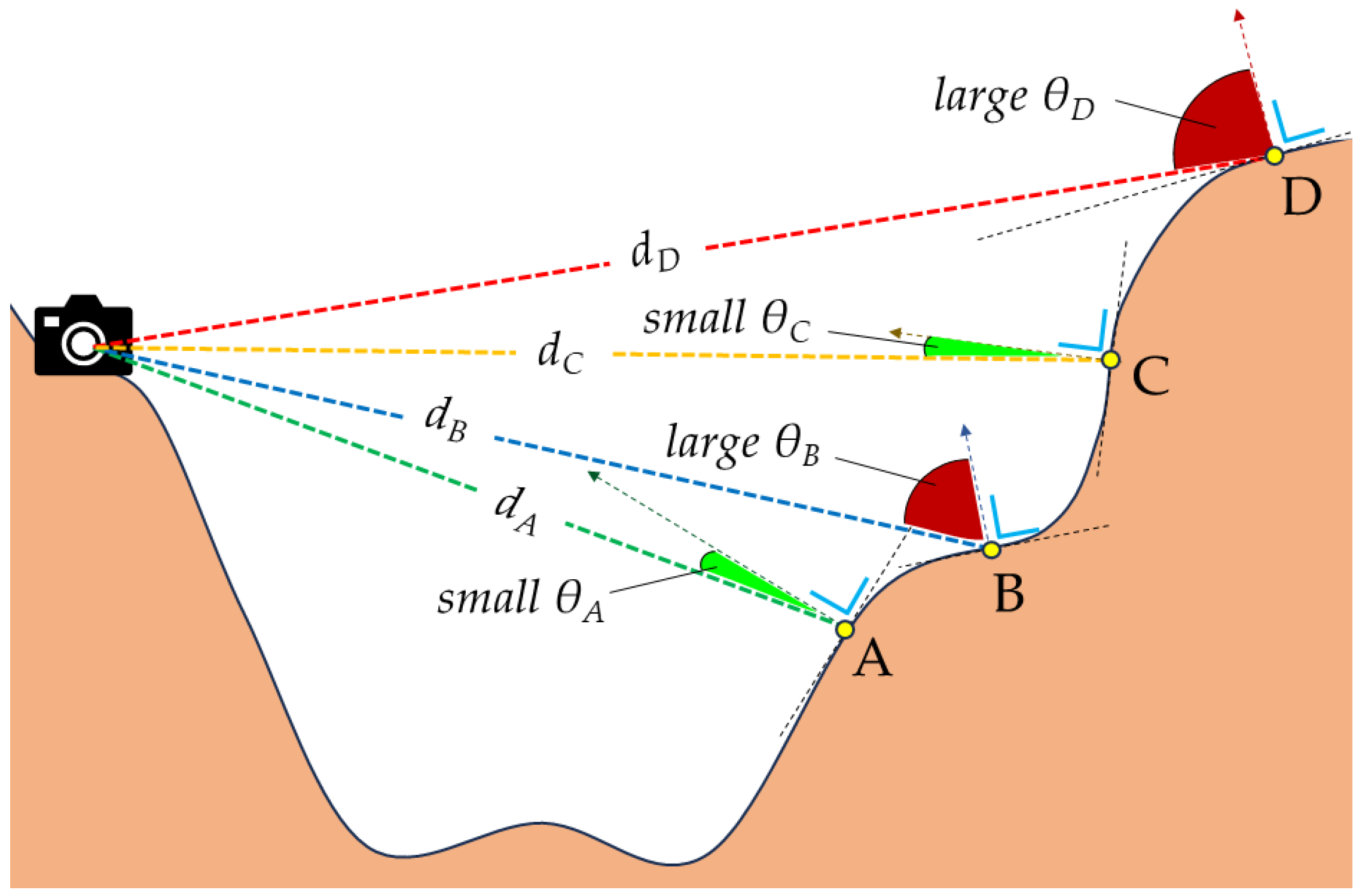
  • Accuracy and precision: the accuracy and precision of the photogrammetric system are lower than those of the other methods (i.e., RTS and GNSS) and are highly dependent on the distance and orientation of the monitored surface relative to the shooting direction of the cameras.
  • Directional resolution: while the photogrammetric system effectively captures transversal displacements relative to the direction of shooting, it is less capable of maintaining the same resolution in monitoring displacements directed toward the camera as the RTS method.
Other site-specific considerations that affect the reliability of the measurements include the following:
  • Surface conditions: vegetated surfaces in general are not suitable to be monitored adequately with image correlation algorithms because of the occurrence of artifactual shifts due to vegetation growth and movement of leaves and stems with wind. Also, snow-covered surfaces are not suitable. Even if DIPHORM uses filters that help to reduce these problems, unvegetated dry areas should be preferred.
  • Environmental conditions: heavy rainfalls, shadows, reflections, and fog and clouds can significantly reduce the quality of photogrammetric monitoring with results that are difficult to estimate. A good selection of photos at the start, such as the one proposed, can help reduce this problem appreciably.
  • The DIPHORM method appears particularly suitable for measuring the displacements of medium-slow, low-vegetated landslides, with an orthogonal view of the slope and with displacements that are preferentially transversal-oriented (i.e., not along the line of sight). DIPHORM is reliable in providing a general view of landslide displacements in a spatially dense manner, where the accuracy of the individual measurement is not as important compared to understanding the overall spatial and temporal trend. In this sense, the DIPHORM technique is not intended as an alternative to the other traditional topographic systems. Instead, combining both the photogrammetric system and the RTS method (and/or GNSS receivers, laser scanner surveys, GB-InSAR surveys), as implemented at the Sant’Andrea landslide, leverages the advantages of both methods and provides a more comprehensive understanding of landslide dynamics. Further developments of the method could include the use of multiple cameras simultaneously, even with different optics, and integrating other techniques to update the 3D surface on which the measurements are projected more frequently and automatically.
The results of adaptable and cost-effective monitoring, such as DIPHORM, could be very useful in the future in the implementation of early warning systems or as input for prediction models, such as those proposed by [30,47]. The availability of spatially and temporally dense information, even if not highly precise, yet ensuring an accurate relative comparison of displacement measurements both in space and time, provides a valuable dataset for training artificial intelligence models. These models can be designed to predict abnormal and particularly concerning landslide behaviors by correlating the collected measurements with environmental factors such as rainfall, temperature, and humidity. Additionally, DIPHORM data can be compared with that obtained from other innovative techniques, such as satellite imagery or ground-based measurements, to build a sufficiently redundant and validated monitoring system.
The Sant’Andrea landslide presents optimal conditions for monitoring with DIPHORM. While it should be noted that with this technology it is possible to optimize the location and type of cameras and the time intervals of image acquisition, it will be important in the future to consider other landslide types in order to better define the range of applicability of this method. For example, landslides that are characterized by dense vegetation, or fog, or have significant surface changes over time or movement predominantly along the line of sight of the cameras present challenging conditions that are more favorable to other established technologies. Therefore, although DIPHORM is indeed flexible and adaptable to various site conditions, it is important to note that it cannot be adequate in all scenarios.

Author Contributions

Conceptualization, L.B., F.G., D.V. and E.C.; methodology, L.B., F.G., D.V. and E.C.; data curation, L.B., F.G., D.V., E.C. and A.P.; formal analysis, L.B., F.G. and D.V.; software, L.B., F.G., D.V. and E.C.; investigation, L.B., F.G., D.V. and E.C.; validation, L.B. and D.V.; visualization, L.B., F.G., D.V. and E.C.; writing—original draft preparation, L.B., F.G., D.V., E.C. and A.P.; writing—review and editing, L.B., F.G. and E.C.; funding acquisition, L.B., S.C. and A.G.; resources, L.B., F.G., S.C. and A.G.; supervision, S.C., A.G. and L.B. All authors have read and agreed to the published version of the manuscript.

Funding

This study was financially supported by the Fondazione Cariverona (https://www.fondazionecariverona.org ID: 11170, cod.SIME 2019.0430.209) through the research grant titled “Monitoring of Natural Hazards and Protective Structures Using Computer Vision Techniques for Environmental Safety and Preservation” and by the Veneto Region through the grant “Scientific Support for the Characterization of Hydrogeological Risk and the Evaluation of the Effectiveness of Interventions Related to the Landslide Phenomenon of Busa del Cristo in Perarolo di Cadore (BL) through the Development of Predictive Geo-Hydrological Models”. Open Access Funding by the University of Vienna.

Data Availability Statement

The monitoring measurements obtained from the DIPHORM technique are available at https://geotechlab.dicea.unipd.it/wp-content/uploads/perarolo/main.html (accessed on 25 August 2024). The meteorological data can be freely downloaded from https://www.ambienteveneto.it. Other data will be made available on reasonable request.

Conflicts of Interest

The authors declare no conflicts of interest. The funders had no role in the design of this study; in the collection, analyses, or interpretation of data; in the writing of the manuscript; or in the decision to publish the results.

References

  1. Angeli, M.-G.; Pasuto, A.; Silvano, S. A Critical Review of Landslide Monitoring Experiences. Eng. Geol. 2000, 55, 133–147. [Google Scholar] [CrossRef]
  2. Cola, S.; Gabrieli, F.; Marcato, G.; Pasuto, A.; Simonini, P. Evolutionary Behaviour of the Tessina Landslide. Riv. Ital. Geotec. 2016, 50, 51–70. [Google Scholar]
  3. Dunnicliff, J. Geotechnical Instrumentation for Monitoring Field Performance; A Wiley-Interscience Publication; Wiley: New York, NY, USA, 1993; ISBN 978-0-471-00546-9. [Google Scholar]
  4. Marr, P.; Jiménez Donato, Y.A.; Carraro, E.; Kanta, R.; Glade, T. The Role of Historical Data to Investigate Slow-Moving Landslides by Long-Term Monitoring Systems in Lower Austria. Land 2023, 12, 659. [Google Scholar] [CrossRef]
  5. Crosta, G.B.; Di Prisco, C.; Frattini, P.; Frigerio, G.; Castellanza, R.; Agliardi, F. Chasing a Complete Understanding of the Triggering Mechanisms of a Large Rapidly Evolving Rockslide. Landslides 2014, 11, 747–764. [Google Scholar] [CrossRef]
  6. Carlà, T.; Tofani, V.; Lombardi, L.; Raspini, F.; Bianchini, S.; Bertolo, D.; Thuegaz, P.; Casagli, N. Combination of GNSS, Satellite InSAR, and GBInSAR Remote Sensing Monitoring to Improve the Understanding of a Large Landslide in High Alpine Environment. Geomorphology 2019, 335, 62–75. [Google Scholar] [CrossRef]
  7. Kasperski, J.; Delacourt, C.; Allemand, P.; Potherat, P.; Jaud, M.; Varrel, E. Application of a Terrestrial Laser Scanner (TLS) to the Study of the Séchilienne Landslide (Isère, France). Remote Sens. 2010, 2, 2785–2802. [Google Scholar] [CrossRef]
  8. Delacourt, C.; Allemand, P.; Berthier, E.; Raucoules, D.; Casson, B.; Grandjean, P.; Pambrun, C.; Varel, E. Remote-Sensing Techniques for Analysing Landslide Kinematics: A Review. Bull. Soc. Géol. Fr. 2007, 178, 89–100. [Google Scholar] [CrossRef]
  9. Prokop, A.; Panholzer, H. Assessing the Capability of Terrestrial Laser Scanning for Monitoring Slow Moving Landslides. Nat. Hazards Earth Syst. Sci. 2009, 9, 1921–1928. [Google Scholar] [CrossRef]
  10. Bitelli, G.; Dubbini, M.; Zanutta, A. Terrestrial Laser Scanning and Digital Photogrammetry Techniques to Monitor Landslide Bodies. Int. Arch. Photogramm. Remote Sens. Spat. Inf. Sci. 2004, 35, 246–251. [Google Scholar]
  11. Teza, G.; Galgaro, A.; Zaltron, N.; Genevois, R. Terrestrial Laser Scanner to Detect Landslide Displacement Fields: A New Approach. Int. J. Remote Sens. 2007, 28, 3425–3446. [Google Scholar] [CrossRef]
  12. Kromer, R.A.; Abellán, A.; Hutchinson, D.J.; Lato, M.; Chanut, M.-A.; Dubois, L.; Jaboyedoff, M. Automated Terrestrial Laser Scanning with Near-Real-Time Change Detection—Monitoring of the Séchilienne Landslide. Earth Surf. Dyn. 2017, 5, 293–310. [Google Scholar] [CrossRef]
  13. Caduff, R.; Schlunegger, F.; Kos, A.; Wiesmann, A. A Review of Terrestrial Radar Interferometry for Measuring Surface Change in the Geosciences. Earth Surf. Process. Landf. 2015, 40, 208–228. [Google Scholar] [CrossRef]
  14. Tarchi, D.; Casagli, N.; Fanti, R.; Leva, D.D.; Luzi, G.; Pasuto, A.; Pieraccini, M.; Silvano, S. Landslide Monitoring by Using Ground-Based SAR Interferometry: An Example of Application to the Tessina Landslide in Italy. Eng. Geol. 2003, 68, 15–30. [Google Scholar] [CrossRef]
  15. Monserrat, O.; Crosetto, M.; Luzi, G. A Review of Ground-Based SAR Interferometry for Deformation Measurement. ISPRS J. Photogramm. Remote Sens. 2014, 93, 40–48. [Google Scholar] [CrossRef]
  16. Stumpf, A.; Malet, J.-P.; Allemand, P.; Pierrot-Deseilligny, M.; Skupinski, G. Ground-Based Multi-View Photogrammetry for the Monitoring of Landslide Deformation and Erosion. Geomorphology 2015, 231, 130–145. [Google Scholar] [CrossRef]
  17. Livio, F.A.; Bovo, F.; Gabrieli, F.; Gambillara, R.; Rossato, S.; Martin, S.; Michetti, A.M. Stability Analysis of a Landslide Scarp by Means of Virtual Outcrops: The Mt. Peron Niche Area (Masiere Di Vedana Rock Avalanche, Eastern Southern Alps). Front. Earth Sci. 2022, 10, 863880. [Google Scholar] [CrossRef]
  18. Kromer, R.; Walton, G.; Gray, B.; Lato, M.; Group, R. Development and Optimization of an Automated Fixed-Location Time Lapse Photogrammetric Rock Slope Monitoring System. Remote Sens. 2019, 11, 1890. [Google Scholar] [CrossRef]
  19. Blanch, X.; Abellan, A.; Guinau, M. Point Cloud Stacking: A Workflow to Enhance 3D Monitoring Capabilities Using Time-Lapse Cameras. Remote Sens. 2020, 12, 1240. [Google Scholar] [CrossRef]
  20. Giacomini, A.; Thoeni, K.; Santise, M.; Diotri, F.; Booth, S.; Fityus, S.; Roncella, R. Temporal-Spatial Frequency Rockfall Data from Open-Pit Highwalls Using a Low-Cost Monitoring System. Remote Sens. 2020, 12, 2459. [Google Scholar] [CrossRef]
  21. Travelletti, J.; Delacourt, C.; Allemand, P.; Malet, J.-P.; Schmittbuhl, J.; Toussaint, R.; Bastard, M. Correlation of Multi-Temporal Ground-Based Optical Images for Landslide Monitoring: Application, Potential and Limitations. ISPRS J. Photogramm. Remote Sens. 2012, 70, 39–55. [Google Scholar] [CrossRef]
  22. Motta, M.; Gabrieli, F.; Corsini, A.; Manzi, V.; Ronchetti, F.; Cola, S. Landslide Displacement Monitoring from Multi-Temporal Terrestrial Digital Images: Case of the Valoria Landslide Site. In Landslide Science and Practice; Margottini, C., Canuti, P., Sassa, K., Eds.; Springer: Berlin/Heidelberg, Germany, 2013; pp. 73–78. ISBN 978-3-642-31444-5. [Google Scholar]
  23. Roncella, R.; Forlani, G.; Fornari, M.; Diotri, F. Landslide Monitoring by Fixed-Base Terrestrial Stereo-Photogrammetry. ISPRS Ann. Photogramm. Remote Sens. Spat. Inf. Sci. 2014, II–5, 297–304. [Google Scholar] [CrossRef]
  24. Stanier, S.A.; Blaber, J.; Take, W.A.; White, D.J. Improved Image-Based Deformation Measurement for Geotechnical Applications. Can. Geotech. J. 2016, 53, 727–739. [Google Scholar] [CrossRef]
  25. Take, W.A. Thirty-Sixth Canadian Geotechnical Colloquium: Advances in Visualization of Geotechnical Processes through Digital Image Correlation. Can. Geotech. J. 2015, 52, 1199–1220. [Google Scholar] [CrossRef]
  26. White, D.J.; Take, W.A.; Bolton, M.D. Soil Deformation Measurement Using Particle Image Velocimetry (PIV) and Photogrammetry. Géotechnique 2003, 53, 619–631. [Google Scholar] [CrossRef]
  27. Aryal, A.; Brooks, B.A.; Reid, M.E.; Bawden, G.W.; Pawlak, G.R. Displacement Fields from Point Cloud Data: Application of Particle Imaging Velocimetry to Landslide Geodesy. J. Geophys. Res. Earth Surf. 2012, 117, 2011JF002161. [Google Scholar] [CrossRef]
  28. Brezzi, L.; Carraro, E.; Pasa, D.; Teza, G.; Cola, S.; Galgaro, A. Post-Collapse Evolution of a Rapid Landslide from Sequential Analysis with FE and SPH-Based Models. Geosciences 2021, 11, 364. [Google Scholar] [CrossRef]
  29. Brezzi, L.; Carraro, E.; Gabrieli, F.; Santa, G.D.; Cola, S.; Galgaro, A. Propagation Analysis and Risk Assessment of an Active Complex Landslide Using a Monte Carlo Statistical Approach. IOP Conf. Ser. Earth Environ. Sci. 2021, 833, 012130. [Google Scholar] [CrossRef]
  30. Teza, G.; Cola, S.; Brezzi, L.; Galgaro, A. Wadenow: A Matlab Toolbox for Early Forecasting of the Velocity Trend of a Rainfall-Triggered Landslide by Means of Continuous Wavelet Transform and Deep Learning. Geosciences 2022, 12, 205. [Google Scholar] [CrossRef]
  31. Reu, P. Stereo-Rig Design: Lens Selection—Part 3. Exp. Tech. 2013, 37, 1–3. [Google Scholar] [CrossRef]
  32. Hartley, R.; Zisserman, A. Multiple View Geometry in Computer Vision, 2nd ed.; Cambridge University Press: Cambridge, UK, 2004; ISBN 978-0-521-54051-3. [Google Scholar]
  33. Westoby, M.J.; Brasington, J.; Glasser, N.F.; Hambrey, M.J.; Reynolds, J.M. ‘Structure-from-Motion’ Photogrammetry: A Low-Cost, Effective Tool for Geoscience Applications. Geomorphology 2012, 179, 300–314. [Google Scholar] [CrossRef]
  34. Heikkila, J.; Silven, O. A Four-Step Camera Calibration Procedure with Implicit Image Correction. In Proceedings of the IEEE Computer Society Conference on Computer Vision and Pattern Recognition, San Juan, PR, USA, 17–19 June 1997; pp. 1106–1112. [Google Scholar]
  35. Zhang, Z. A Flexible New Technique for Camera Calibration. IEEE Trans. Pattern Anal. Mach. Intell. 2000, 22, 1330–1334. [Google Scholar] [CrossRef]
  36. De La Escalera, A.; Armingol, J.M. Automatic Chessboard Detection for Intrinsic and Extrinsic Camera Parameter Calibration. Sensors 2010, 10, 2027–2044. [Google Scholar] [CrossRef]
  37. Piermattei, L.; Carturan, L.; De Blasi, F.; Tarolli, P.; Dalla Fontana, G.; Vettore, A.; Pfeifer, N. Suitability of Ground-Based SfM–MVS for Monitoring Glacial and Periglacial Processes. Earth Surf. Dyn. 2016, 4, 425–443. [Google Scholar] [CrossRef]
  38. Chen, Y.; Medioni, G. Object Modelling by Registration of Multiple Range Images. Image Vis. Comput. 1992, 10, 145–155. [Google Scholar] [CrossRef]
  39. González-Aguilera, D.; Rodríguez-Gonzálvez, P.; Gómez-Lahoz, J. An Automatic Procedure for Co-Registration of Terrestrial Laser Scanners and Digital Cameras. ISPRS J. Photogramm. Remote Sens. 2009, 64, 308–316. [Google Scholar] [CrossRef]
  40. Lichti, D.; Gordon, S.; Stewart, M.; Franke, J.; Tsakiri, M. Comparison of Digital Photogrammetry and Laser Scanning. In Proceedings of the International Society for Photogrammetry and Remote Sensing, Graz, Austria, 9 September 2002; pp. 39–44. [Google Scholar]
  41. Szegedy, C.; Liu, W.; Jia, Y.; Sermanet, P.; Reed, S.; Anguelov, D.; Erhan, D.; Vanhoucke, V.; Rabinovich, A. Going Deeper with Convolutions. In Proceedings of the 2015 IEEE Conference on Computer Vision and Pattern Recognition (CVPR), Boston, MA, USA, 7–12 June 2015; pp. 1–9. [Google Scholar]
  42. Zhou, B.; Khosla, A.; Lapedriza, A.; Torralba, A.; Oliva, A. Places: An Image Database for Deep Scene Understanding. arXiv 2016, arXiv:1610.02055. [Google Scholar] [CrossRef]
  43. Pan, B.; Qian, K.; Xie, H.; Asundi, A. Two-Dimensional Digital Image Correlation for in-Plane Displacement and Strain Measurement: A Review. Meas. Sci. Technol. 2009, 20, 062001. [Google Scholar] [CrossRef]
  44. Gabrieli, F.; Corain, L.; Vettore, L. A Low-Cost Landslide Displacement Activity Assessment from Time-Lapse Photogrammetry and Rainfall Data: Application to the Tessina Landslide Site. Geomorphology 2016, 269, 56–74. [Google Scholar] [CrossRef]
  45. Teza, G.; Pesci, A.; Genevois, R.; Galgaro, A. Characterization of Landslide Ground Surface Kinematics from Terrestrial Laser Scanning and Strain Field Computation. Geomorphology 2008, 97, 424–437. [Google Scholar] [CrossRef]
  46. Wei, S.; Wang, C.; Yang, Y.; Wang, M. Physical and Mechanical Properties of Gypsum-Like Rock Materials. Adv. Civ. Eng. 2020, 2020, 3703706. [Google Scholar] [CrossRef]
  47. Liu, Y.; Brezzi, L.; Liang, Z.; Gabrieli, F.; Zhou, Z.; Cola, S. Image Analysis and LSTM Methods for Forecasting Surficial Displacements of a Landslide Triggered by Snowfall and Rainfall. Landslides 2024, 1–17. [Google Scholar] [CrossRef]
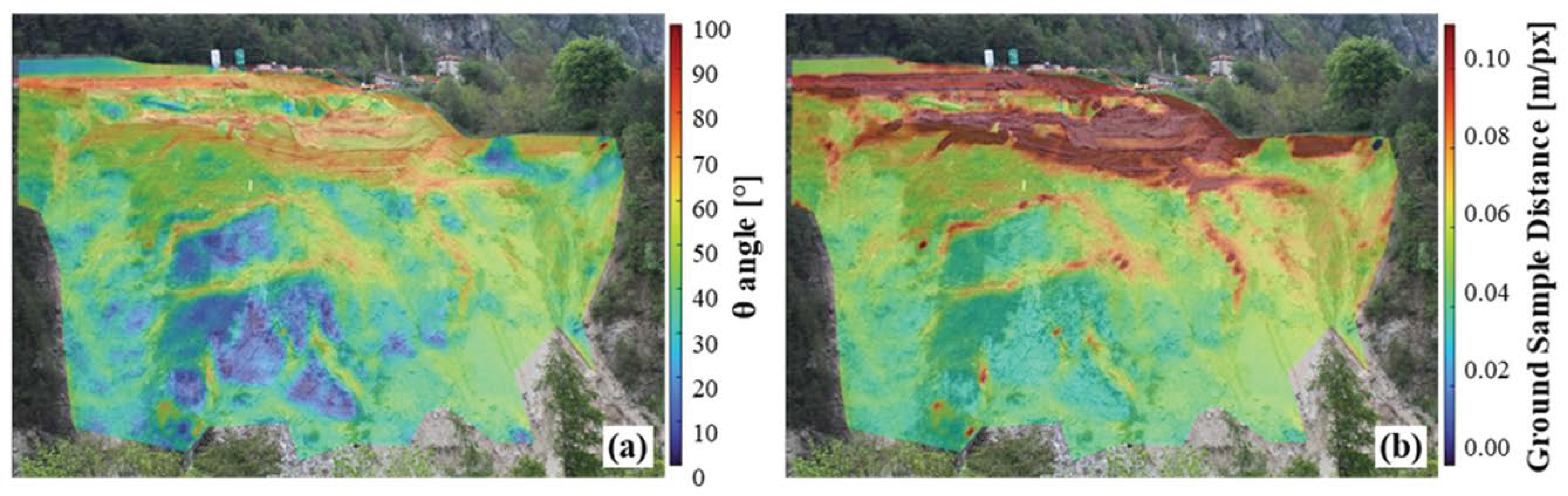
Figure 1. Logical scheme of the algorithm at the base of DIPHORM.
Remotesensing 16 03199 g001
Figure 2. Examples of hardware configurations for photogrammetric systems. (a) Representation of the individual hardware components; (be) examples of on-site installations available online.
Remotesensing 16 03199 g002
Figure 3. DIPHORM photo-taking, calibration, and processing workflow: (a) Image acquisition from multiple views (including fixed view C2); (b) feature detection, matching of key points, and bundle adjustment for intrinsic parameters and camera pose estimation; (c) image undistortion and calculation of the depth map of the scene based on the dense point cloud previously obtained or with an external registered point cloud (e.g., laser scanner point cloud); (d) collection of time-lapse images from position C2; (e) digital image correlation (NCC metric) applied to a grid of patches on the images; and (f) 3D projection of the 2D displacement on the depth map of the scene. C1, C2, …C5 and P1, P2, …P5 refer to the camera positions and the corresponding photos in the calibration phase. Xj refer to the key points used for matching and t0, t1,…tn to the time steps of the image sequence.
Remotesensing 16 03199 g003
Figure 4. Examples of unusable images selected by the Convolutional Neural Network for the presence of (a) rain, (b) snow, (c) fog, (d) glare, (e) darkness, and (f) objects in the image.
Remotesensing 16 03199 g004
Figure 5. Examples of image ratings given by the Convolutional Neural Network: (a) presence of large shadow casts = rate 2; (b) presence of slight shadows = rate 3; (c) rate 4; and (d) rate 5 (highest rate).
Remotesensing 16 03199 g005
Figure 6. Two-dimensional graphical representation of the θ angle between the line of sight and the normal vector to the slope surface to the monitored terrain surface. Points A and C are characterized by a small θ angle, while points B and D are characterized by a large θ angle, close to 90°. However, points A and B are closer to the camera and thus may have better resolution (m/px) compared to points C and D, which are farther away.
Remotesensing 16 03199 g006
Figure 7. (a) Areal view of the Sant’Andrea landslide site and Perarolo di Cadore village (NE Italy) taken from UAV survey in March 2022; (b) front view of the slope on 8 June 2021 just before the collapse induced with explosives.
Remotesensing 16 03199 g007
Figure 8. Cumulative displacements were measured for some target points (Table 2).
Remotesensing 16 03199 g008
Figure 9. Maps of the total displacement field over the periods (a) April to May 2021 and (b) August to September 2021. Horizontal displacements are reported as arrows in each target position.
Remotesensing 16 03199 g009
Figure 10. (a) Aerial view of the landslide with camera locations; (b,c) view of one of the monitoring systems; GPS surveys of (d) a corner and (e) a reference sphere, both located on the big scarp edge of the slope; and (f) laser scanning survey of the landslide.
Remotesensing 16 03199 g010
Figure 11. (a) The θ angle map and (b) GSD map for the scene framed by one of the three cameras.
Remotesensing 16 03199 g011
Figure 12. Contour maps of monthly total displacement obtained with DIPHORM in the period 3 May 2021–30 September 2022: (a) May 2021; (b) June 2021; (c) July 2021; (d) August 2021; (e) September 2021; (f) October 2021; (g) February 2022; (h) April 2022; (i) May 2022; (j) June 2022; (k) July 2022; (l) August 2022; (m) September 2022. The monthly cumulative rainfalls (in mm) are also reported in the bottom left corner of each photo.
Remotesensing 16 03199 g012
Figure 13. Image of the landslide taken on 3 May 2021 from the camera’s point of view with the topographic target location. The blue dots (PR1 and PR2) correspond to the targets destroyed in the collapse of June 2021, the green ones (N3, P1, and N10) to areas where movements are very low, and the red ones highlight the targets characterized by a high movement rate.
Remotesensing 16 03199 g013
Figure 14. Cumulative displacement trends obtained by photogrammetric technique and topographic monitoring for: (a) N3 target; (b) P1 target; (c) N10 target; (d) PR1 target; (e) PR2 target; (f) PR3 target; (g) PR4 target; (h) PR5 target; (i) GPS1 target; (j) N6 target; (k) P3 target; (l) P28 target; (m) P24 target; (n) C1 target. The values based on the image analysis are obtained on the Region of Interest (ROI) positioned in the areas surrounding the topographic targets considered.
Remotesensing 16 03199 g014
Figure 15. Scheme of the camera field of view for the N6 prism projected on the ground surface compared to the total station view.
Remotesensing 16 03199 g015
Figure 16. Monthly contour maps of average velocity in cm/day of six selected ROIs obtained from the photo analysis for the period 3 May 2021–31 July 2022: (a) May 2021; (b) June 2021; (c) July 2021; (d) August 2021; (e) September 2021; (f) October 2021; (g) May 2022; (h) June 2022; (i) July 2022.
Remotesensing 16 03199 g016
Figure 17. Cumulative mean displacements for (a) ROIs 1 and 2, (b) ROIs 3 and 4, and (c) ROIs 5 and 6, shown in Figure 16, in the period from 3 May 2021 to 30 September 2022. The average velocities are also reported on the graphs.
Remotesensing 16 03199 g017
Figure 18. Comparison of the cumulative monthly displacement distributions in the months of (a) May and August 2021 for ROI 2 and (b) June 2021 and June 2022 for ROI 3; (c) legend of the violin plot.
Remotesensing 16 03199 g018
Table 1. The θ angles, distances (d) from the monitoring system, and GSD (Ground Sampling Distance) for points A, B, C, and D as represented in Figure 6.
PointθdGSD
ASmallShortSmall
BLargeShortMedium
CSmallLongMedium
DLargeLongLarge
Table 2. Annual total displacements measured at some targets placed on the slope. Note that the recording period may vary, and the installation date is indicated at the bottom of the table.
Target NameAnnual Total Displacement (cm)
201420152016201720182019202020212022
N3 2----0.1 (166d)0.40.40.80.4
P10.70.40.51.00.70.71.31.30.7
N10 2----0.3 (166d)0.40.40.80.4
GPS1 1--17.3 (226d)35.667.9113.8260.6390.688.5
N6 2----22.2 (166d)n.a.n.a.181.177.5
P333.426.527.728.847.9n.a.n.a.114.21n.a.
P28 1--15.9 (226d)28.651.575.5172.5276.465.8
P24 1--16.4 (226d)31.266.081.0177.6278.862.8
C1 3------54.9 (28d)287.743.6
P436.727.931.434.962.5103.2232.0345.987.4
P836.328.330.032.352.881.0186.0352.1101.4
P1334.727.527.527.944.371.3166.2297.272.3
P1934.424.228.132.054.685.4187.1283.758.8
PR1 4-------88.4 (64d)n.a.
PR2 4-------53.9 (64d)n.a.
PR3 5-------132.7 (257d)72.3
PR4 5-------120.5 (257d)67.2
PR5 5-------111.3 (257d)57.4
Installed on 19 May 2016 (1); 18 July 2018 (2); 3 December 2020 (3); 6 April 2021 (4) (lasted 64 days); and 18 April 2021 (5).
Disclaimer/Publisher’s Note: The statements, opinions and data contained in all publications are solely those of the individual author(s) and contributor(s) and not of MDPI and/or the editor(s). MDPI and/or the editor(s) disclaim responsibility for any injury to people or property resulting from any ideas, methods, instructions or products referred to in the content.

