Through-Wall Imaging Using Low-Cost Frequency-Modulated Continuous Wave Radar Sensors

Abstract

Many fields of human activity benefit from the ability to create images of obscured objects placed behind walls and to map their displacement in a noninvasive way. Usually, imaging devices like Synthetic Aperture Radars (SARs) and Ground-Penetrating Radars (GPRs) use expensive dedicated electronics which results in prohibitive prices. This paper presents the experimental implementation and the results obtained from an imaging system capable of performing SAR imaging and interferometric displacement mapping of targets located behind walls, as well as 3D GPR imaging using a low-cost general-purpose radar sensor. The proposed solution uses for the RF section of the system a K-band microwave radar sensor module implementing Frequency-Modulated Continuous Wave (FMCW) operation. The low-cost sensor was originally intended for simple presence detection and ranging for domestic applications. The proposed system was tested in several scenarios and proved to operate as intended for a fraction of the cost of a commercial imaging device. In one scenario, it was able to detect and locate a 15 cm-diameter fire-extinguisher located at a distance of 3.5 m from the scanning system and 1.6 m behind a 3 cm-thick MDF (medium-density fiberboard) wall with cm-level accuracy. In a second test, the proposed system was used to perform interferometric displacement measurements, and it was capable of determining the displacement of a metal case with sub-millimeter accuracy. In a third experiment, the system was used to construct a 3D image of the inside of a wood table with cm-level resolution.

1. Introduction

Non-destructive imaging of objects situated behind optically opaque walls can be achieved by means of penetrating radio waves [1,2] in the form of Ground-Penetrating Radars (GPRs). Like all radars, GPRs generate radio waves and analyze the echoes resulted from the reflections of these waves at discontinuities in the tested medium [3]. This technology is very mature and has been successfully applied in many fields of human activity like geological surveys [4,5], archeology [6], military mine detection [7] and civil engineering applications [8]. It is difficult for an inexperienced user to interpret typical GPR images due to their poor resolution. The pathway for improving the resolution of the image is to create synthetic large apertures of the GPR antennas by mathematically processing the raw image using algorithms inspired by the airborne Synthetic Aperture Radar (SAR). The scientific literature presents several successful implementations of Synthetic Aperture GPR focusing techniques [9,10,11,12]. Although very well established, the GPR technology uses expensive dedicated electronics which results in prohibitive prices making it inaccessible to the amateur archeologist or domestic user.

This paper addresses the high costs issue of current GPRs, which are based on custom built expensive radio frequency sections, by proposing two low-cost scanning systems based on highly available general-purpose radar modules.

The operating frequency of the proposed systems lies in the K-band at 24 GHz. This limits the penetration depth in wet soil to only a couple of centimeters, making it useful only for detecting superficial buried objects. However, typical walls and floors can be penetrated easily by this frequency, making the proposed system useful for finding objects or construction elements encased in walls or behind walls, in non-conductive boxes or beneath floors. The detection depth is dependent to the radar cross-section (RCS) of the targets. For a metal plate 10 by 10 cm and 1 mm thick, the reliable detection depth in dry wood, brick walls, concrete or stone is 50 cm.

A similar commercial system for through-wall imaging using radio waves is Walabot [13], a wideband imaging radar for collecting frontal images in free space and in through-wall conditions. The solution proposed in this paper uses 40 mW of RF power in the 24–25 GHz band, while Walabot emits only 0.14 mW in the 6.3–8 GHz band, resulting in improved penetration depth for the proposed system. The software v1.2.2 provided with Walabot is not capable of generating GPR-style images or performing interferometric processing.

For commercial 60 GHz radar modules [14], current regulations limit the transmitted power to maximum 10 mW, while the propagation loss due to oxygen molecules has a maximum at this frequency, resulting in lower penetration capabilities compared to the system proposed in this paper. Wood is opaque at this frequency, rendering through-wall imaging practically impossible.

Compared to the above mentioned commercially available counterparts, the systems proposed in this paper have increased penetration capability due to their higher transmitted power, and lower manufacturing costs.

The objective of this paper is to develop and test low-cost imaging systems capable of performing SAR imaging and interferometric displacement mapping of targets located behind walls, as well as 3D GPR imaging using a highly affordable general-purpose radar sensor and some simple electronics.

2. Materials and Methods

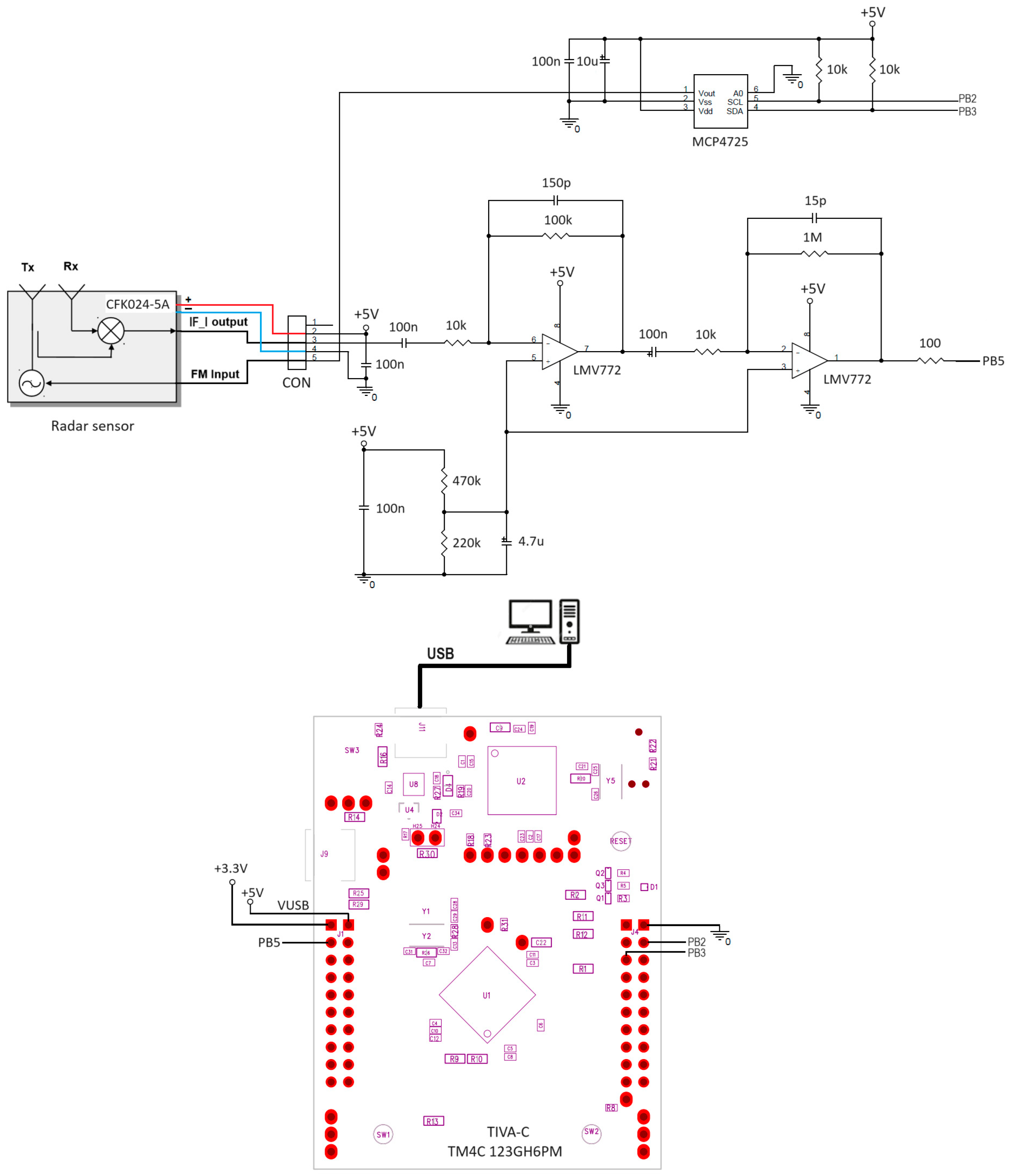
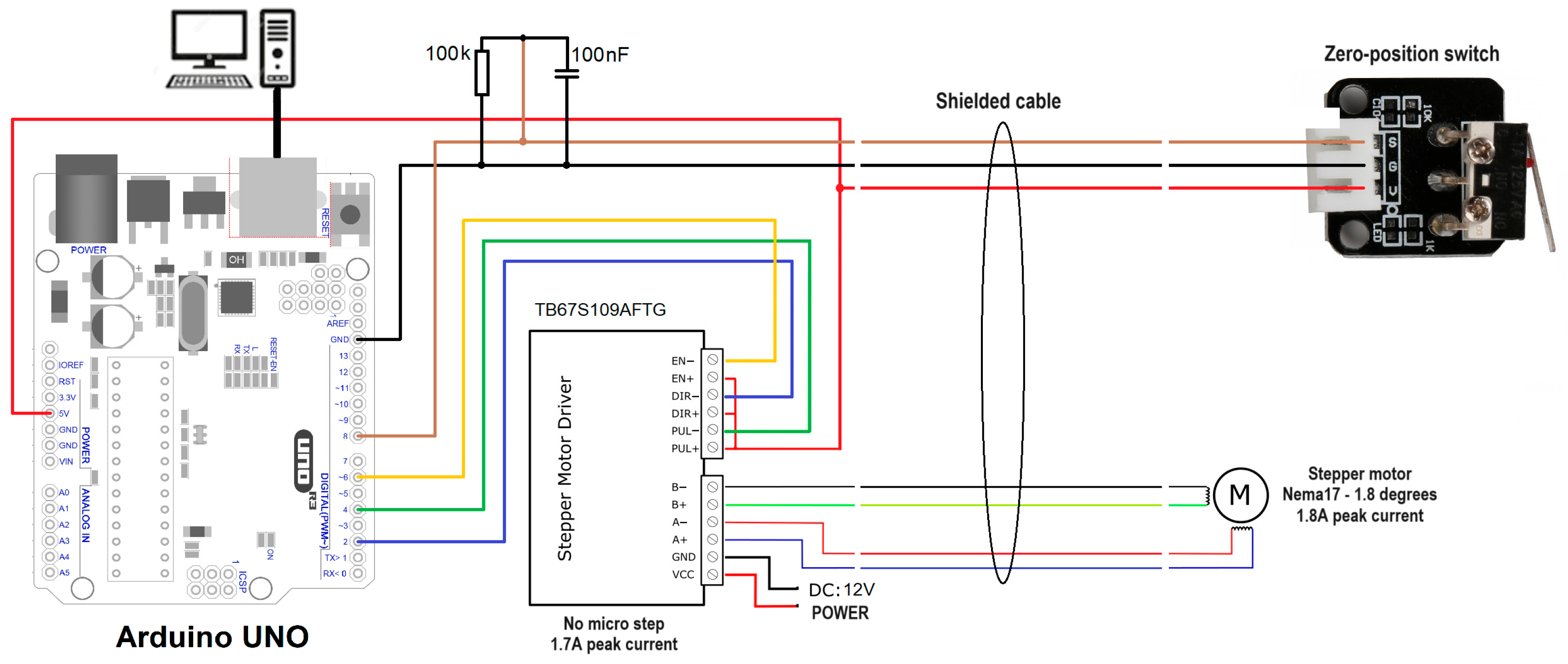
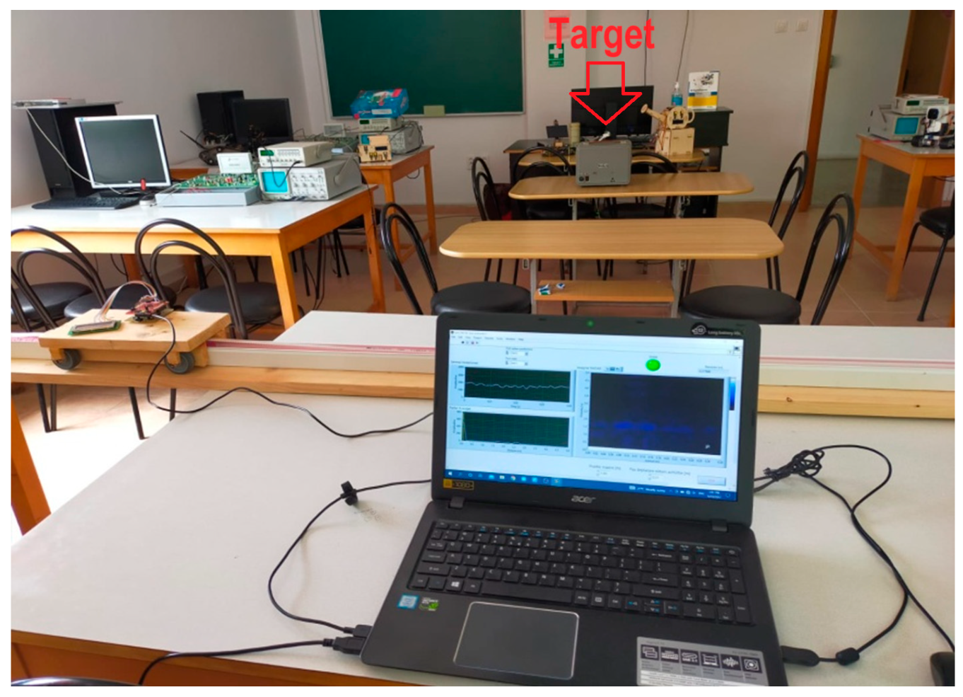
2.1. GB-SAR Implementation

The first proposed implementation of the imaging system takes the form of a Ground-Based Synthetic Aperture Radar (GB-SAR). The low-cost Frequency-Modulated Continuous Wave (FMCW) radar circuit has the schematic presented in Figure 1. For the RF section, the low-cost K-band FMCW radar sensor CFK024-5A from Fevas, China was used. The linear ramp 0–2 V signal needed for modulating the transmitted frequency of the radar in order to generate a linear chirp is created by means of the Microchip Technology MCP4725 Digital to Analogue Converter. The output of the radar sensor is amplified, shifted and filtered by the Texas Instruments LMV772 Operational Amplifier. The digital section of the proposed system is implemented by the Texas Instruments TIVA-C TM4C-123GH6PM development board. The sampling rate used for digitizing the signal obtained at the output of the amplifier is 20,580 Hz with 12 bits of resolution. The frequency domain behavior of the amplifier is shown in Figure 2.

In order to move the radar module in a straight line during the scanning procedure, a computer-controlled rail system was implemented. It will be named the radar positioning system. The rail uses an Arduino Uno board that continuously listens for positions expressed in millimeters sent from the computer through a USB connection, the same computer the radar module is connected to. When a position followed by a New Line ASCII character is received, the Arduino computes the number of steps needed by the stepper motor to move the carriage to the received position and sends the appropriate signal sequence to the Stepper Motor Driver. In order to calibrate the zero position of the rail at the beginning of the scanning procedure, a switch is placed at the start of the rail. The schematic diagram of the rail electronics is presented in Figure 3. The practical implementation of the rail is depicted in Figure 4. The program running on the Texas Instruments TIVA-C TM4C-123GH6PM development board, the digital section of the radar module, implements the flowchart detailed in Figure 5. The program running on the PC implements the flowchart presented in Figure 6. The s_cor(n) correction signal is the radar output IF signal obtained in a reflection-free environment, the anechoic chamber. Range argument in r(range) is the discrete range or distance vector. FFT designates the Fast Fourier Transform.

In order to improve the azimuth resolution of the image created by the radar system, thanks to the coherency of the radar sensor module, synthetic aperture focusing can be applied on the stored raw data. The proposed SAR focusing algorithm is a backprojection-type algorithm operating in time-domain, inspired by [15,16].

The derivation of the focusing algorithm starts with the FMCW radar signal model. The transmitted waveform has the expression:

s_t(t) = cos (2πf_st − πγt²),

(1)

where time t is the time variable 0 < t < T, T is the sweep duration, f_s is the starting frequency of the sweep, γ is the sweep rate γ = B/T and B is the bandwidth of the sweep.

The received echo is a scaled time-delayed copy of the transmitted signal. If we ignore the amplitude scaling, the received signal is:

s_r(t) = s_t(t − t_d) = cos [2πf_s(t − t_d) − πγ(t − t_d)²],

(2)

where t_d is the time delay.

The radar sensor mixes the transmitted signal with the received signal. After filtering out the high frequency undesired components and neglecting the ½ scaling, the signal at the radar module IF (intermediate frequency) output, assuming a real valued (not complex) output, is:

s_IF(t) = cos (−2πf_st_d − πγt_d² + 2πγt_dt).

(3)

During the scan, the radar repeats this measurement while moving on a straight path, the rail, with constant distance increments. The position of the radar on the path is:

x = n Δx,

(4)

where Δx is the position increment on the rail, and n designates the index of the radar position. For simplicity, we assume the radar path starts from the origin of the coordinate system and y = z = 0, so that the radar position is completely determined only by x.

By accounting for the fact that the electromagnetic waves travel at the speed of light and the radar signal travels to the target and then back to the radar, we obtain the following expression for the received signal time delay:

t_d = 2 d(r, x)/c,

(5)

where c is the speed of light and d(r, x) is the distance between the radar located at position x and the reflecting target located at position r(x_t, y_t, z_t) and can be computed from the Pythagorean theorem as d(r, x) = $\sqrt{{({\mathrm{x}}_{\mathrm{t}}-\mathrm{x})}^2+{{\mathrm{y}}_{\mathrm{t}}}^2+{{\mathrm{z}}_{\mathrm{t}}}^2}$.

By introducing Equation (5) in Equation (3), the radar sensor output signal can be written:

$${\mathrm{s}}_{\mathrm{IF}}(\mathrm{t})=\cos [-\frac{4\mathsf{\pi }}{\mathrm{c}}({\mathrm{f}}_{\mathrm{s}}-\mathsf{\gamma }\mathrm{t}) \mathrm{d}(\mathbf{r},\mathrm{x}) -\frac{4\mathsf{\pi }\mathsf{\gamma }}{{\mathrm{c}}^2}{\mathrm{d}}^2(\mathbf{r},\mathrm{x})].$$

(6)

By neglecting the last term in the cosine function argument, the so-called residual video phase term, and taking into account Equation (4), the IF radar output signal can be written as:

$${\mathrm{s}}_{\mathrm{IF}}(\mathrm{n}, \mathrm{t})=\cos [-\frac{4\mathsf{\pi }}{\mathrm{c}} ({\mathrm{f}}_{\mathrm{s}}-\mathsf{\gamma }\mathrm{t}) \mathrm{d}(\mathbf{r},\mathrm{n}\mathsf{\Delta }\mathrm{x})].$$

(7)

After sampling by the ADC (Analog to Digital) converter, the IF signal becomes:

s_IF(n, m) = s_IF(n, mT_s),

(8)

where t = mT_s, T_s is the sampling period of the ADC, and m is the sample index.

The most straight-forward method for generating a SAR-focused image is to apply a matched filtering. For each pixel in the output image, we can calculate what the measured IF signal would have been if there was a target located at that pixel location r. Matched filtering the measured signal with the expected signal will produce a high value when the measurement matches the expectation. We need to repeat the filtering process for each pixel in the output in order to obtain the focused image.

The mathematical expression for filtering one pixel is:

$$\mathrm{I}(\mathbf{r})={\sum }_{\mathrm{n}=0}^{\mathrm{N}-1}{\sum }_{\mathrm{m}=0}^{\mathrm{M}-1}{\mathrm{s}}_{\mathrm{I}\mathrm{F}}\left(\mathrm{n},\mathrm{m}\right){\mathrm{s}}_{\mathrm{r}\mathrm{e}\mathrm{f}}\left(\mathrm{n},\mathrm{m}\right),$$

(9)

where I(r) is the focused image matrix, r is the location of the pixel, N is the total number of radar sweeps or scan positions, M is the total number of samples of the IF signal and s_ref[n, m] is the so-called reference function or expected IF response for an isotropic point scatterer:

$${\mathrm{S}}_{\mathrm{ref}}(\mathrm{n}, \mathrm{m})=\cos [-\frac{4\mathsf{\pi }}{\mathrm{c}}({\mathrm{f}}_{\mathrm{s}}-\mathsf{\gamma }\mathrm{m}{\mathrm{T}}_{\mathrm{s}}) \mathrm{d}(\mathbf{r},\mathrm{n}\mathsf{\Delta }\mathrm{x})].$$

(10)

In order to obtain a complex image suitable for interferometric processing, the complex representation of the reference function will be used:

$${\mathrm{S}}_{\mathrm{ref}\_\mathrm{c}}(\mathrm{n}, \mathrm{m})=\exp [\mathrm{j}\frac{4\mathsf{\pi }}{\mathrm{c}}({\mathrm{f}}_{\mathrm{s}}-\mathsf{\gamma }\mathrm{m}{\mathrm{T}}_{\mathrm{s}}) \mathrm{d}(\mathbf{r},\mathrm{n}\mathsf{\Delta }\mathrm{x})].$$

(11)

We can implement the focusing algorithm directly by applying iteratively Equation (9) for every pixel in the image. This approach is called the Matched Filter Algorithm. It works very well in terms of focused image quality, but it needs a huge number of arithmetic operations, making it unsuitable for large images. It has a computational complexity of O(n⁴).

Fortunately, there is a way to reduce the complexity to O(n³) by factoring the complex reference function into two parts:

$${\mathrm{S}}_{\mathrm{ref}\_\mathrm{c}}(\mathrm{n}, \mathrm{m})=\mathrm{e}\mathrm{x}\mathrm{p} [\mathrm{j}\frac{4\mathsf{\pi }{\mathrm{f}}_{\mathrm{s}}}{\mathrm{c}}\mathrm{d}(\mathbf{r},\mathrm{n}\mathsf{\Delta }\mathrm{x})]·\mathrm{e}\mathrm{x}\mathrm{p}[-\mathrm{j}\frac{4\mathsf{\pi }}{\mathrm{c}}\mathsf{\gamma }\mathrm{m}{\mathrm{T}}_{\mathrm{s}} \mathrm{d}(\mathbf{r},\mathrm{n}\mathsf{\Delta }\mathrm{x})].$$

(12)

Now we can rewrite Equation (9) as:

$$\mathrm{I}(\mathbf{r})={\sum }_{\mathrm{n}=0}^{\mathrm{N}-1} \mathrm{e}\mathrm{x}\mathrm{p} [\mathrm{j}\frac{4\mathsf{\pi }{\mathrm{f}}_{\mathrm{s}}}{\mathrm{c}}\mathrm{d}(\mathbf{r},\mathrm{n}\mathsf{\Delta }\mathrm{x})]{\sum }_{\mathrm{m}=0}^{\mathrm{M}-1}{\mathrm{s}}_{\mathrm{I}\mathrm{F}}\left(\mathrm{n},\mathrm{m}\right) \mathrm{e}\mathrm{x}\mathrm{p} [-\mathrm{j}\frac{4\mathsf{\pi }}{\mathrm{c}}\mathsf{\gamma }\mathrm{m}{\mathrm{T}}_{\mathrm{s}} \mathrm{d}(\mathbf{r},\mathrm{n}\mathsf{\Delta }\mathrm{x})].$$

(13)

Equation (13) can now be rewritten using the Direct Discrete Fourier Transform, which, if implemented using the efficient algorithm called Fast Fourier Transform (FFT), reduces the computational complexity by one order of magnitude.

The definition of the Direct FFT applied to s_IF(n, m) is:

$${\mathrm{S}}_{\mathrm{IF}}[\mathrm{n}, \mathrm{k}]={\sum }_{\mathrm{m}=0}^{\mathrm{M}-1}{\mathrm{s}}_{\mathrm{I}\mathrm{F}}\left(\mathrm{n},\mathrm{m}\right) \mathrm{e}\mathrm{x}\mathrm{p} (-\mathrm{j}\frac{2\mathsf{\pi }\mathrm{k}\mathrm{m}}{\mathrm{M}})$$

(14)

.

In order to write Equation (13) in terms of Direct FFT, we need to solve for the index k in the equation:

$$-\mathrm{j}\frac{2\mathsf{\pi }\mathrm{k}\mathrm{m}}{\mathrm{M}}=-\mathrm{j}\frac{4\mathsf{\pi }}{\mathrm{c}}\mathsf{\gamma }\mathrm{m}{\mathrm{T}}_{\mathrm{s}} \mathrm{d}(\mathbf{r},\mathrm{n}\mathsf{\Delta }\mathrm{x}).$$

(15)

This leads to:

$$\mathrm{k}=\frac{2}{\mathrm{c}}\mathrm{M}\mathsf{\gamma }{\mathrm{T}}_{\mathrm{s}} \mathrm{d}(\mathbf{r},\mathrm{n}\mathsf{\Delta }\mathrm{x}).$$

(16)

Using γ = B/T and T_s = T/M, we can rewrite k as:

$$\mathrm{k}=\frac{2}{\mathrm{c}}\mathrm{M}\frac{\mathrm{B}}{\mathrm{T}}\frac{\mathrm{T}}{\mathrm{M}} \mathrm{d}(\mathbf{r},\mathrm{n}\mathsf{\Delta }\mathrm{x})=\frac{2\mathrm{B}}{\mathrm{c}} \mathrm{d}(\mathbf{r},\mathrm{n}\mathsf{\Delta }\mathrm{x}).$$

(17)

Using k, we can rewrite Equation (13) in terms of Direct FFT as:

$$\mathrm{I}(\mathbf{r})={\sum }_{\mathrm{n}=0}^{\mathrm{N}-1}\mathrm{e}\mathrm{x}\mathrm{p} [\mathrm{j}\frac{4\mathsf{\pi }{\mathrm{f}}_{\mathrm{s}}}{\mathrm{c}} \mathrm{d}(\mathbf{r},\mathrm{n}\mathsf{\Delta }\mathrm{x})] {\mathrm{s}}_{\mathrm{I}\mathrm{F}}[\mathrm{n},\frac{2\mathrm{B}}{\mathrm{c}}\mathrm{d}\left(\mathbf{r},\mathrm{n}\mathsf{\Delta }\mathrm{x}\right)],$$

(18)

where S_IF[n, k] is the Direct Fourier transform of s_IF[n, m] along the second axis.

Due to the fact that k = $\frac{2\mathrm{B}}{\mathrm{c}}$ d(r, nΔx) index in Equation (18) is not always a whole number and FFT computes only for whole k numbers, an interpolation step is needed.

Equation (18) applied to each pixel in the final image represents the backprojection SAR focusing algorithm.

Each pixel in the focused image is a complex number, so that the image can be used for interferometry applications.

In order to reduce complexity and costs, the hardware solution proposed in this paper uses only one output of the radar sensor, IF_I, so the real-valued IF signal situation discussed above applies. Also, the transmitted signal is a down-chirp, as was the case in the derivation above.

The IF_Q output of the radar module is left unconnected and is not represented in the schematics.

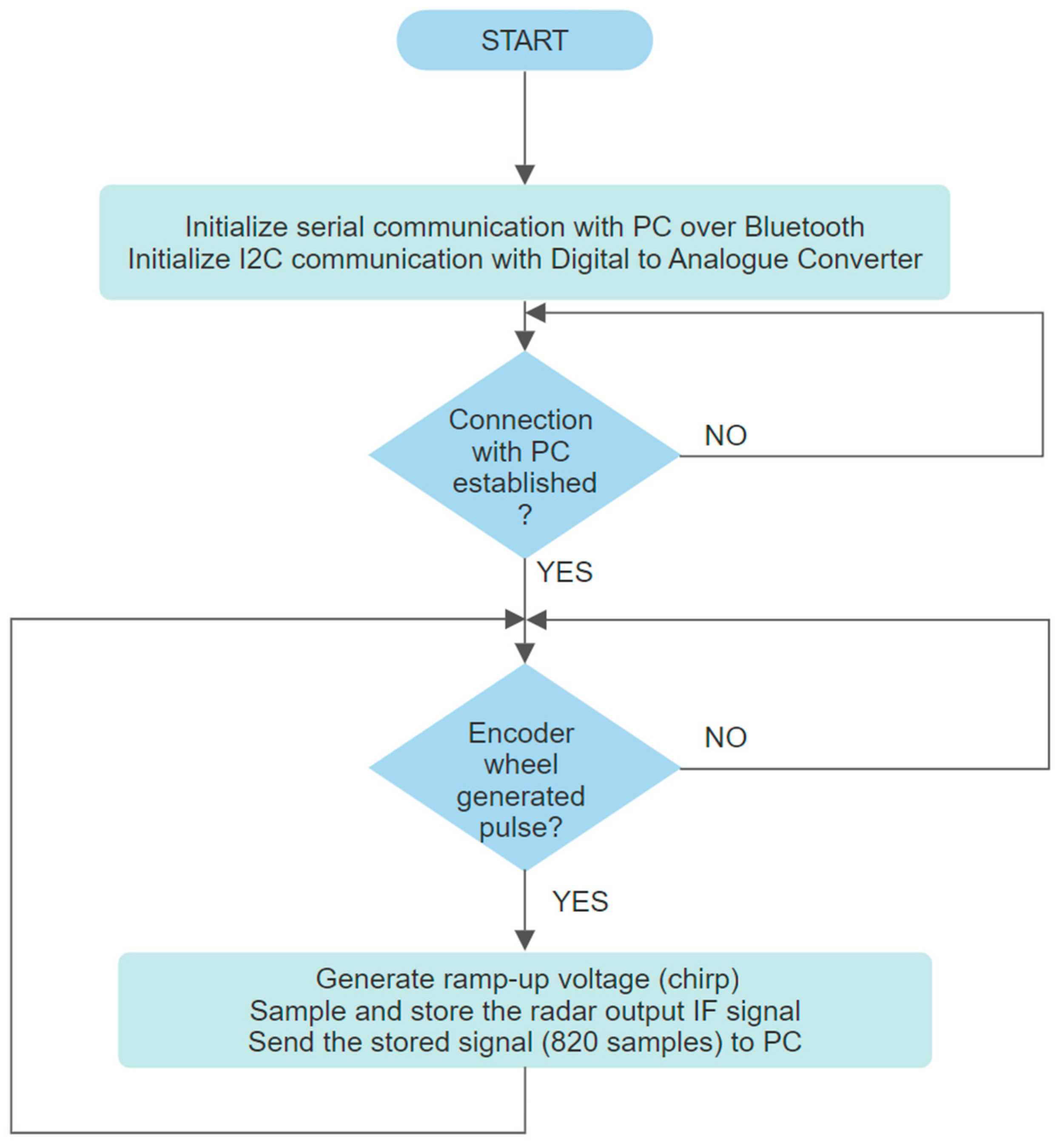
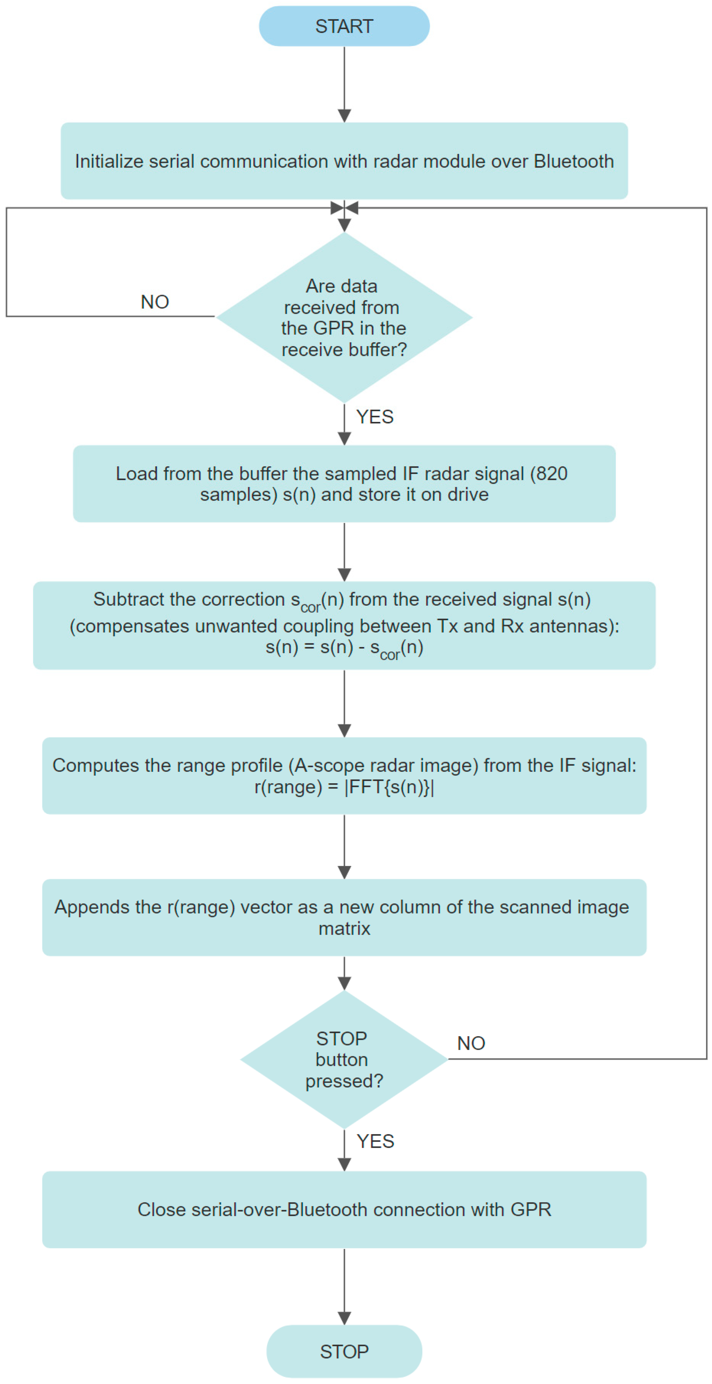
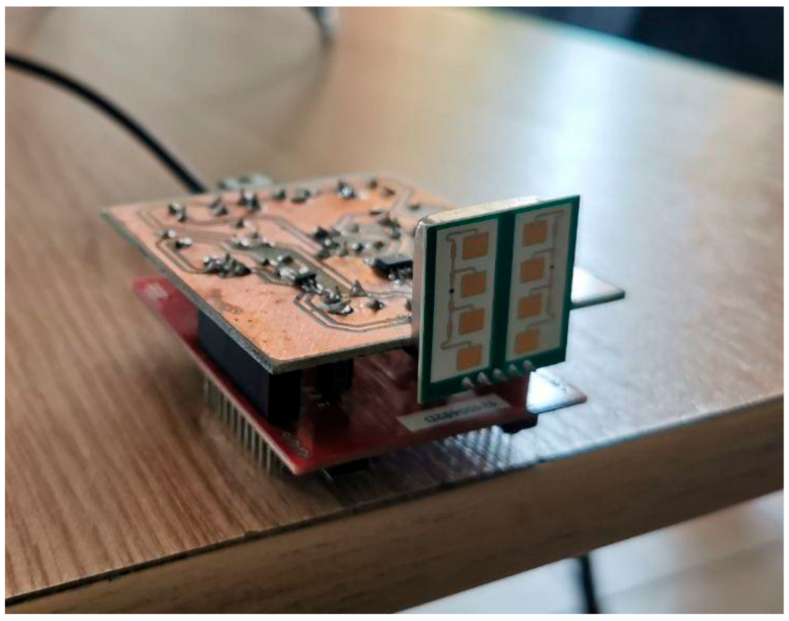
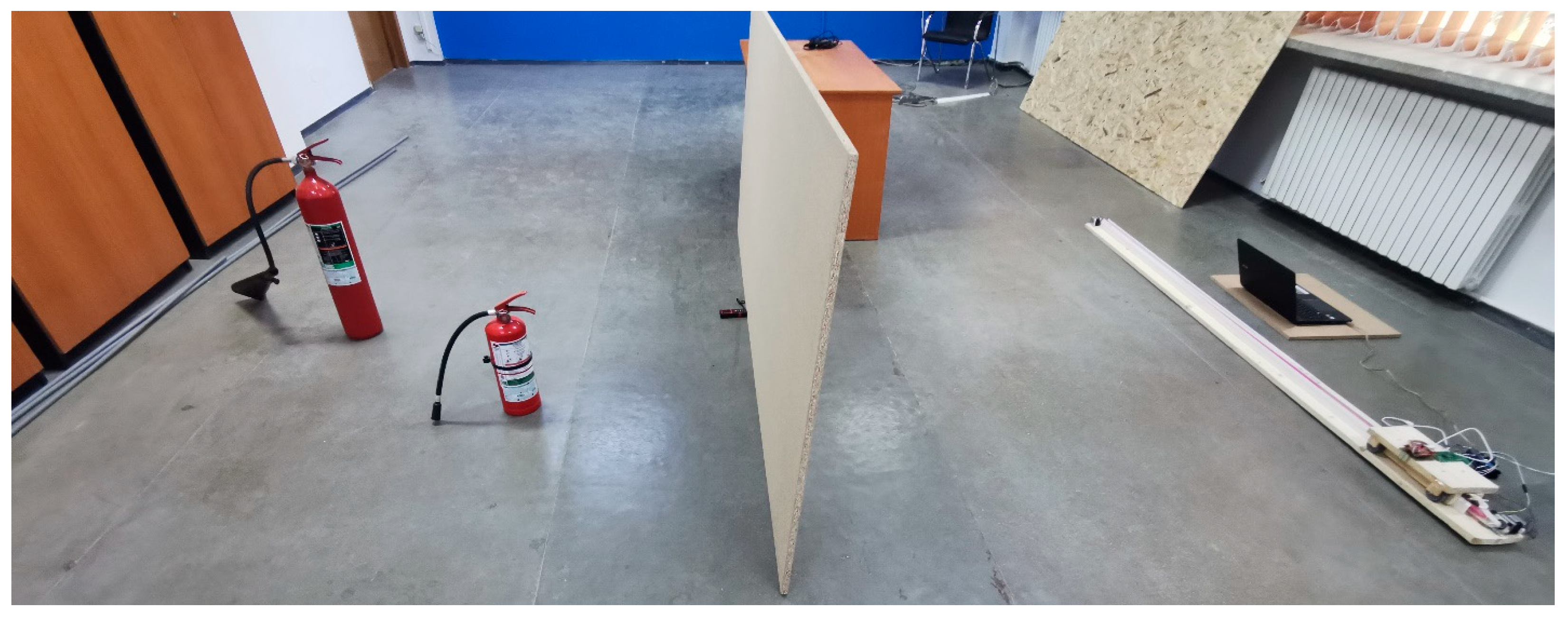
2.2. GPR Implementation

The second proposed implementation of the imaging system takes the form of a hand-held Ground-Penetrating Radar (GPR). It builds upon the hardware of the GB-SAR implementation by adding a Bluetooth module for wireless connection with the PC, an encoder wheel and optocoupler for determining the radar position and a battery (powerbank). The new radar circuit has the schematic presented in Figure 7. The encoder wheel has a diameter of 3.82 cm and 4 equally spaced holes, which gives 4 pulses at the output of the U-shaped optocoupler for every revolution. This means a pulse for every 3 cm traveled by the GPR. Every pulse triggers a scan producing an A-scope image, so that the azimuth sampling step of the radar image is 3 cm. The practical implementation of the GPR system is presented in Figure 8.

The program running on the TIVA-C TM4C-123GH6PM development board, the digital section of the radar module, implements the flowchart in Figure 9. The program running on the PC implements the flowchart presented in Figure 10. The s_cor(n) correction signal is the radar output IF signal obtained in a reflection-free environment, the anechoic chamber. Range argument in r(range) is the discrete range or distance vector. FFT designates the Fast Fourier Transform.

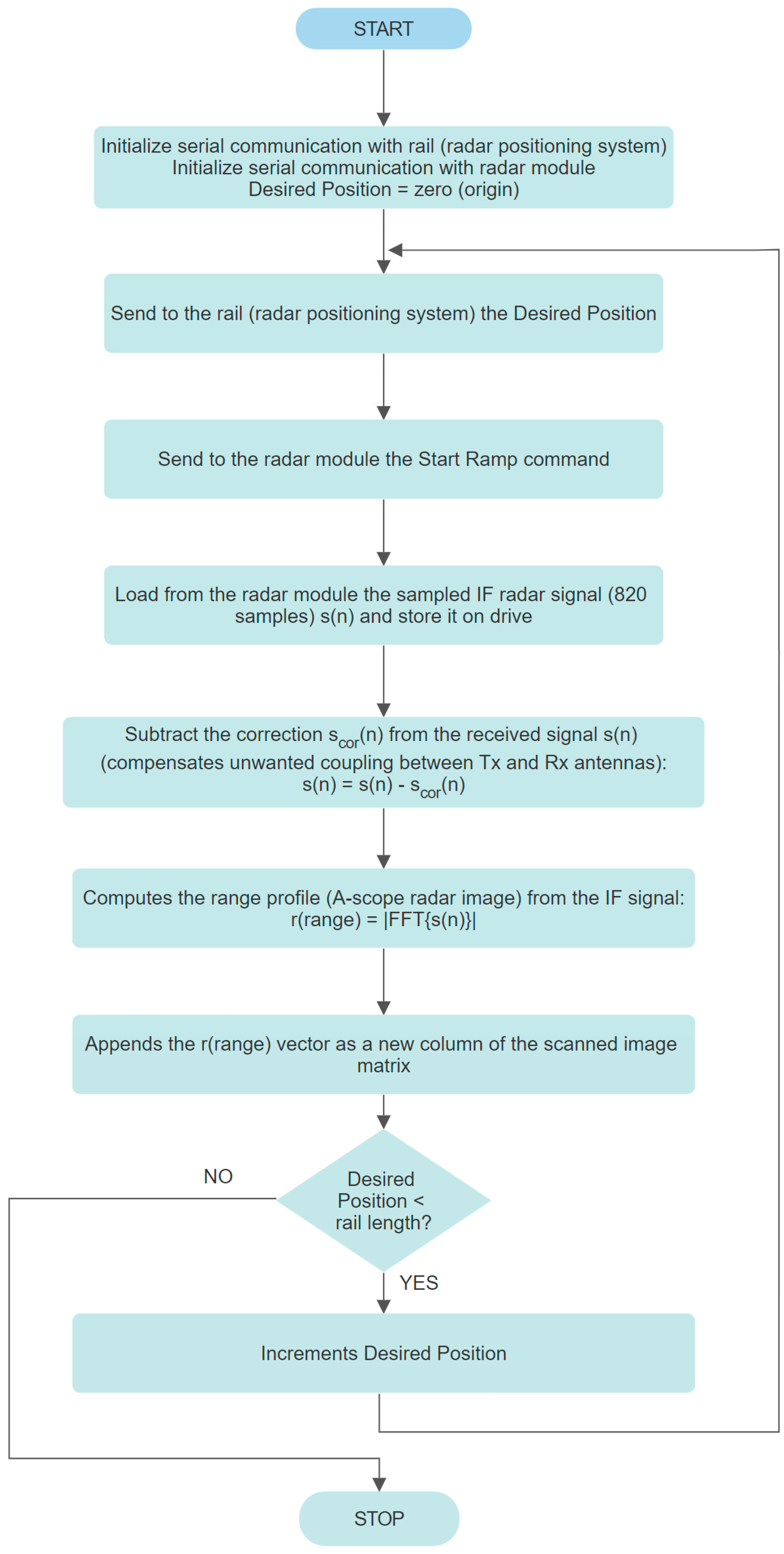
3. Methodology

The GB-SAR implementation performance was tested in two experiments. The first one was designed to test the imaging ability of the system by placing two metal fire extinguishers behind an MDF wall. The raw image was focused by means of the proposed SAR algorithm, and the targets’ positions in the radar image were confronted with real-world tape measurements. The second experiment was designed to test the interferometric capability of the GB-SAR implementation by determining the movement of the metal case target placed in front of the system between two successive scans.

Finally, the GPR implementation was tested by placing a metal case under a wooden table and performing straight-line scans on its top. The raw data were processed and a 3D image of the table inside was created. The image was confronted to the real-world geometry.

4. Results

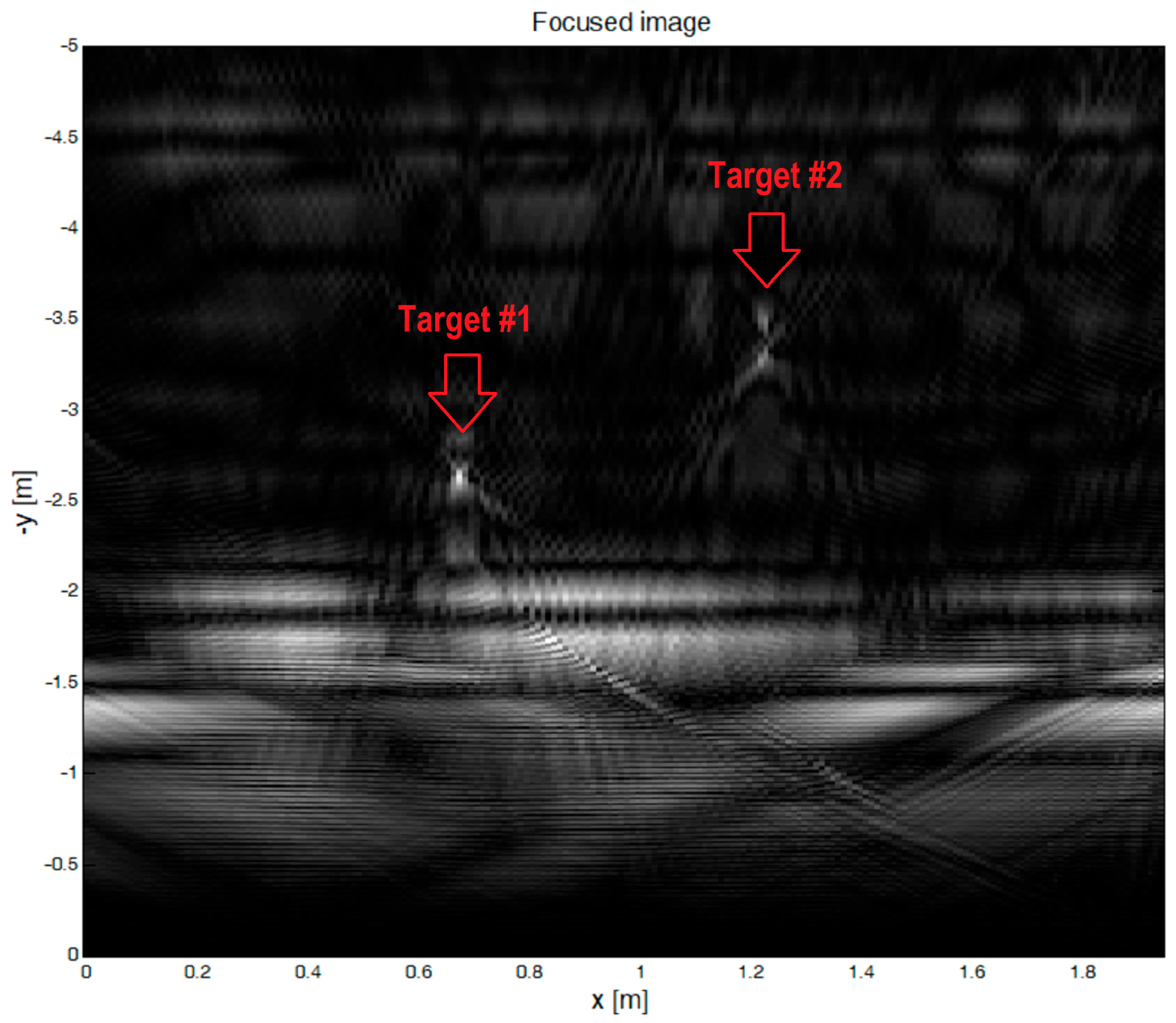
4.1. GB-SAR Results

In Figure 11 the hardware implementation of the GB-SAR radar module is depicted. During the scanning process, it is moved by the carriage on the computer-controlled rail.

The system was tested using the setup described in Figure 12. Two cylindrical metal targets represented by two fire extinguishers were placed behind a 3 cm-thick MDF (medium-density fiberboard) wall.

The real setup image is presented in Figure 13.

The focused radar image obtained from the test setup is depicted in Figure 14.

The two targets are clearly visible in the radar-generated image. The image represents the absolute values of the complex pixels generated by the focusing algorithm. The image is a 2D section situated in a plane perpendicular to the wall. The z coordinate is 0.

The focusing algorithm was configured to take into account the radiation pattern of the radar antennas. When computing the contribution of each radar position to the final image, only the pixels contained in the radar antenna real aperture, an 80 degrees cone, were updated. The sampling step (position increment) on the x axis was 1 cm. The chirp bandwidth B was 685 MHz, giving a range (y axis) resolution of c/2B = 21 cm. The x axis resolution after focusing is about 1 cm. The resulting focused image has a resolution of 1 by 21 cm.

The interferometric capability of the proposed system was tested using the setup from Figure 15.

The analyzed target was the grey metallic box situated directly in front of the radar rail and will appear in the center of the radar image. Two scans have been performed. The box was moved by 3 mm towards the radar between the first and the second scan.

The two images were aligned by successively moving one image and searching the position that maximizes the cross-correlation of the images.

The complex interferogram Inter(r) was computed by multiplying the first focused complex image I₁(r) with the complex conjugate of the aligned second focused complex image I₂(r):

Inter(r) = I₁(r) · conj[I₂(r)].

(19)

The displacement map D(r) was created by multiplying the phases of the interferogram with λ/(4π):

$$\mathrm{D}(\mathbf{r})=\mathrm{a}\mathrm{n}\mathrm{g}\mathrm{l}\mathrm{e}[\mathrm{I}\mathrm{n}\mathrm{t}\mathrm{e}\mathrm{r}(\mathbf{r})]·\frac{\mathsf{\lambda }}{4\mathsf{\pi }}$$

(20)

where λ = c/f_s is the starting wavelength of the transmitted chirp.

The displacement map was filtered so that only the pixels with high values in the interferogram magnitude were plotted. The threshold was 40% of the maximum value of the interferogram magnitude. The filtered displacement map is presented in Figure 16.

The target displacement was estimated to be 0.298 cm, very close to the real 0.3 cm (3 mm) displacement. The error is 0.018 cm, a very satisfactory accuracy for the domestic applications intended for the system.

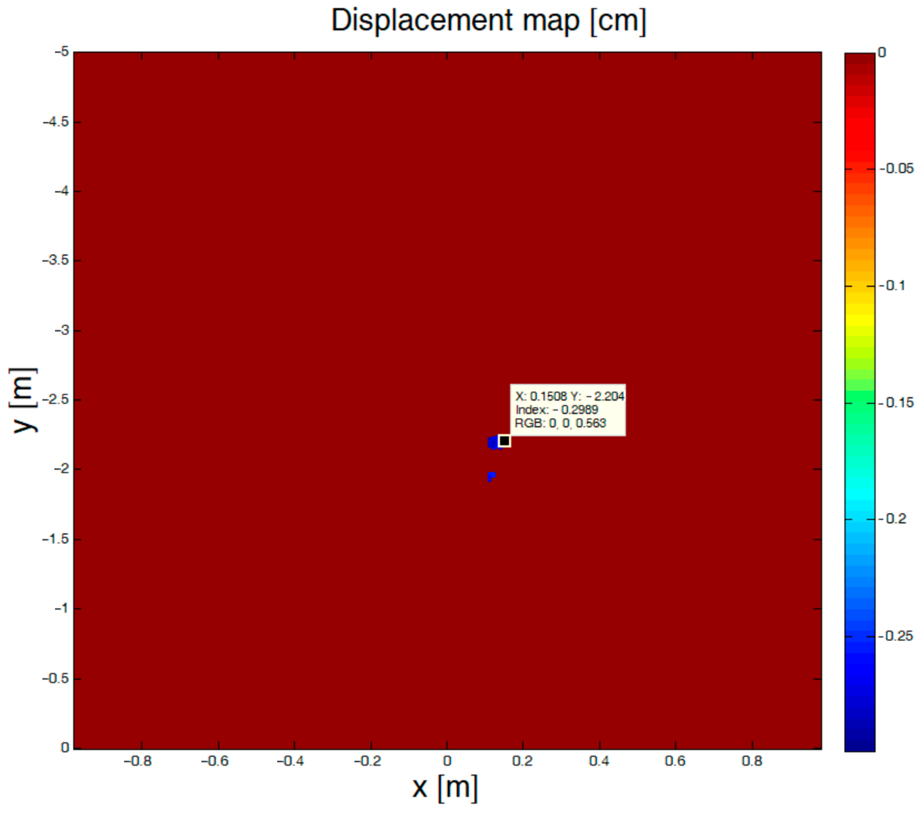
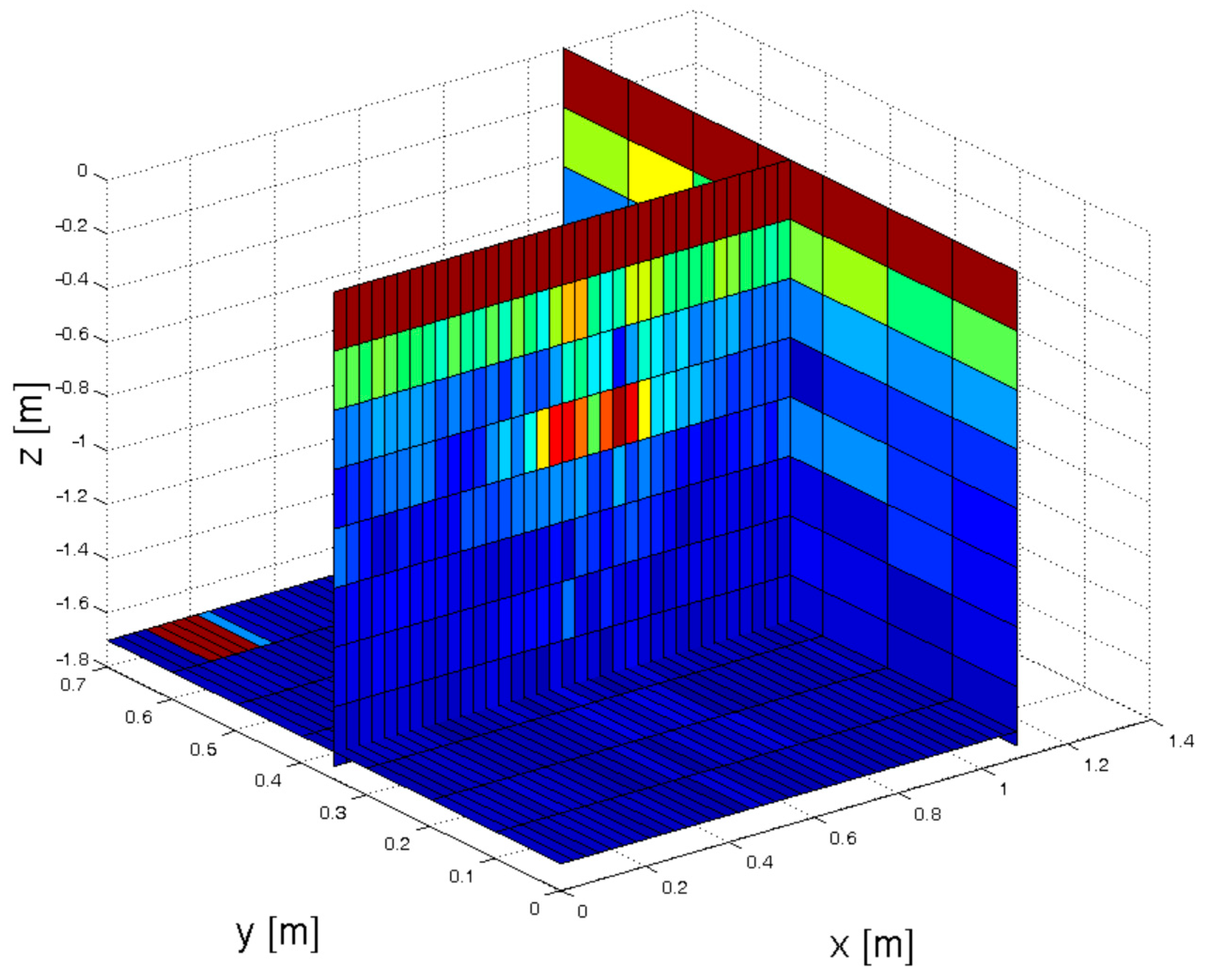
4.2. GPR Results

The hand-held GPR system was tested by performing a scan on top of a wooden table. Under the table, in the center, a metal case 40 cm by 25 cm by 15 cm was positioned on the floor. The height of the table top is 75 cm. The resulting image is presented in Figure 17. The metal case is clearly visible in the center at about 70 cm depth. By moving the GPR on parallel lines, a 3D image was constructed. The image was plotted using three cuts: two at the origins of the X and Z axes, and the last at the middle of the y axis. The table top is also clearly visible in dark red at 0 m depth.

5. Discussion

In this paper, two low-cost systems capable of through-wall imaging were proposed and demonstrated. Both systems use microwave FMCW radar as the key technology. The cost is kept low by using widely available radar modules and general-purpose microcontroller development boards. The operating frequency is 24 GHz, in the unlicensed ISM band. The transmitted power is 40 mW.

Compared to short-range 60 GHz radars available today, which are limited by current regulations to 10 mW of transmitted power, the systems presented in this paper have much higher penetration capabilities. The combination of higher frequency and lower transmit power renders 60 GHz radars completely incapable of penetrating walls.

The first system implements a GB-SAR form and is suitable for generating multiple scans with precisely similar conditions, thus making itself appropriate for interferometric displacement analysis of the obscured targets. The generated image is focused using SAR algorithm for enhancing its resolution, a process that requires precise positioning of the radar obtained by means of the computer-controlled rail. The resolution on the radar movement axis is 1 cm, while the resolution on the perpendicular (range) axis is 21 cm.

By applying interferometrical processing on multiple scanned images, the system is able to measure displacements in the range of mm with sub-millimeter accuracy.

The second implementation is a hand-held portable GPR device which can be used easily for generating ad hoc images of objects placed behind obscuring surfaces or embedded in them. The range resolution is 21 cm in air and reduces proportional to the square root of the dialectical permittivity in other media, giving 5 cm in concrete. The movement axis resolution is range dependent and degrades with increasing range as in typical GPR radars. By performing multiple parallel scans, the resulting cross-sections can be assembled in a 3D image of the analyzed volume.

Both proposed systems were experimentally tested and offered satisfactory results.

6. Conclusions

This paper presents the implementation of two low-cost FMCW radar imaging systems designed to acquire through-wall images. The proposed systems use only general-purpose electronic modules and components. All the signal processing and system parameters are programmable, putting the systems in the category of software-defined radars. This implementation offers maximum of flexibility for modifying the operation of the proposed systems and adapting their functionality to novel usage scenarios.

The operation in the unlicensed 24 GHz frequency band assures compliance with regulations worldwide.

The high transmission power of 40 mW offers a high penetration depth in dry materials like concrete, wood, drywalls, bricks and stone. The penetration depth ranges from tens of cm to meters depending on the radar reflectivity (radar cross-section) of the obscured objects.

The first proposed system uses a computer-operated rail guidance and generates SAR-focused images of 1 by 21 cm resolution in air, with the resolution increasing in higher permittivity materials. Multiple images can be processed interferometrically for generating displacement maps with sub-millimeter accuracy.

The second proposed system is highly portable, being lightweight (<500 g) and small (20 by 10 cm by 10 cm), offers hand-held operation and generates GPR images with 21 cm depth resolution in air. It also offers the possibility of creating 3D images of the scanned volume.

All the above-mentioned assertions have been experimentally demonstrated.

References

- Zhang, W.; Xu, Z.; Guo, S.; Jia, Y.; Wang, L.; He, T.; Shao, H. MIMO through-wall-radar down-view imaging for moving target with ground ghost suppression. Digit. Signal Process. 2023, 134, 103886. [Google Scholar] [CrossRef]
- Saad, M.; Maali, A.; Salah Azzaz, M.; Benssalah, M. An efficient FPGA-based implementation of UWB radar system for through-wall imaging. Int. J. Commun. Syst. 2023, 36, e5510. [Google Scholar] [CrossRef]
- Jol, H.M. Ground Penetrating Radar: Theory and Applications, 1st ed.; Elsevier Science: Amsterdam, The Netherlands, 2009; pp. 1–41. [Google Scholar]
- Davis, J.L.; Annan, P. Ground-Penetrating Radar for High-Resolution Mapping of Soil and Rock Stratigraphy. Geophys. Prospect. 1989, 37, 531–551. [Google Scholar] [CrossRef]
- Blindow, N. Ground Penetrating Radar. In Groundwater Geophysics—A Tool for Hydrology; Kirsch, R., Ed.; Springer: Berlin/Heidelberg, Germany, 2006; pp. 227–252. [Google Scholar] [CrossRef]
- Lowe, K.M.; Wallis, L.A.; Pardoe, C.; Marwick, B.; Clarkson, C.J.; Manne, T.; Smith, M.A.; Fullagar, R. Ground-penetrating radar and burial practices in western Arnhem Land, Australia. Archaeol. Ocean. 2014, 49, 148–157. [Google Scholar] [CrossRef]
- Burr, R.; Schartel, M.; Schmidt, P.; Mayer, W.; Walter, T.; Waldschmidt, C. Design and Implementation of a FMCW GPR for UAV-based Mine Detection. In Proceedings of the IEEE MTT-S International Conference on Microwaves for Intelligent Mobility (ICMIM), Munich, Germany, 15–17 April 2018. [Google Scholar] [CrossRef]
- Wai-Lok Lai, W.; Derobert, X.; Annan, P. A review of Ground Penetrating Radar application in civil engineering: A 30-year journey from Locating and Testing to Imaging and Diagnosis. NDT E Int. 2018, 96, 58–78. [Google Scholar] [CrossRef]
- Yigit, E.; Demirci, S.; Ozdemir, C. Ground Penetrating Radar Image Focusing using Frequency-Wavenumber based Synthetic Aperture Radar Technique. In Proceedings of the 2007 International Conference on Electromagnetics in Advanced Applications, Torino, Italy, 17–21 September 2007; pp. 344–347. [Google Scholar] [CrossRef]
- Ozdemir, C.; Demirci, S.; Yigit, E. Practical Algorithms to Focus B-scan GPR Images: Theory and Application to Real Data. PIERS B 2008, 6, 109–122. [Google Scholar] [CrossRef]
- Baer, C.; Gutierrez, S.; Jebramcik, J.; Barowski, J.; Vega, F.; Rolfes, I. Ground Penetrating Synthetic Aperture Radar Imaging Providing Soil Permittivity Estimation. In Proceedings of the 2017 IEEE MTT-S International Microwave Symposium (IMS), Honolulu, HI, USA, 4–9 June 2017; pp. 1367–1370. [Google Scholar] [CrossRef]
- Ustun, D.; Yigit, E.; Toktas, A.; Sabanci, K.; Duysak, H. GPR Image Focusing Using Matched Filter Algorithm. In Proceedings of the 2018 XXIIIrd International Seminar/Workshop on Direct and Inverse Problems of Electromagnetic and Acoustic Wave Theory (DIPED), Tbilisi, Georgia, 24–27 September 2018; pp. 242–245. [Google Scholar] [CrossRef]
- Walabot Tech Brief. Available online: https://site.walabot.com/docs/walabot-tech-brief-416/ (accessed on 29 March 2024).
- Koul, S.K.; Bharadwaj, R. UWB and 60 GHz Radar Technology for Vital Sign Monitoring, Activity Classification and Detection. In Wearable Antennas and Body Centric Communication; Lecture Notes in Electrical Engineering; Springer: Singapore, 2021; Volume 787. [Google Scholar] [CrossRef]
- Gorham, L.A.; Moore, L.J. SAR image formation toolbox for MATLAB. In Proceedings of the SPIE 7699 Algorithms for Synthetic Aperture Radar Imagery XVII, 769906, SPIE Defense, Security, and Sensing, Orlando, FL, USA, 5–9 April 2010. [Google Scholar] [CrossRef]
- Henrik’s Blog. Available online: https://hforsten.com/backprojection-backpropagation.html (accessed on 9 February 2024).
Disclaimer/Publisher’s Note: The statements, opinions and data contained in all publications are solely those of the individual author(s) and contributor(s) and not of MDPI and/or the editor(s). MDPI and/or the editor(s) disclaim responsibility for any injury to people or property resulting from any ideas, methods, instructions or products referred to in the content. |
© 2024 by the author. Licensee MDPI, Basel, Switzerland. This article is an open access article distributed under the terms and conditions of the Creative Commons Attribution (CC BY) license (https://creativecommons.org/licenses/by/4.0/).
Share and Cite
Paun, M. Through-Wall Imaging Using Low-Cost Frequency-Modulated Continuous Wave Radar Sensors. Remote Sens. 2024, 16, 1426. https://doi.org/10.3390/rs16081426
Paun M. Through-Wall Imaging Using Low-Cost Frequency-Modulated Continuous Wave Radar Sensors. Remote Sensing. 2024; 16(8):1426. https://doi.org/10.3390/rs16081426
Chicago/Turabian StylePaun, Mirel. 2024. "Through-Wall Imaging Using Low-Cost Frequency-Modulated Continuous Wave Radar Sensors" Remote Sensing 16, no. 8: 1426. https://doi.org/10.3390/rs16081426
APA StylePaun, M. (2024). Through-Wall Imaging Using Low-Cost Frequency-Modulated Continuous Wave Radar Sensors. Remote Sensing, 16(8), 1426. https://doi.org/10.3390/rs16081426