Mapping of Clay Montmorillonite Abundance in Agricultural Fields Using Unmixing Methods at Centimeter Scale Hyperspectral Images

Abstract

The composition of clay minerals in soils, and more particularly the presence of montmorillonite (as part of the smectite family), is a key factor in soil swell–shrinking as well as off–road vehicle mobility. Detecting these topsoil clay minerals and quantifying the montmorillonite abundance are a challenge since they are usually intimately mixed with other minerals, soil organic carbon and soil moisture content. Imaging spectroscopy coupled with unmixing methods can address these issues, but the quality of the estimation degrades the coarser the spatial resolution is due to pixel heterogeneity. With the advent of UAV-borne and proximal hyperspectral acquisitions, it is now possible to acquire images at a centimeter scale. Thus, the objective of this paper is to evaluate the accuracy and limitations of unmixing methods to retrieve montmorillonite abundance from very-high-resolution hyperspectral images (1.5 cm) acquired from a camera installed on top of a bucket truck over three different agricultural fields, in Loiret department, France. Two automatic endmember detection methods based on the assumption that materials are linearly mixed, namely the Simplex Identification via Split Augmented Lagrangian (SISAL) and the Minimum Volume Constrained Non-negative Matrix Factorization (MVC-NMF), were tested prior to unmixing. Then, two linear unmixing methods, the fully constrained least square method (FCLS) and the multiple endmember spectral mixture analysis (MESMA), and two nonlinear unmixing ones, the generalized bilinear method (GBM) and the multi-linear model (MLM), were performed on the images. In addition, several spectral preprocessings coupled with these unmixing methods were applied in order to improve the performances. Results showed that our selected automatic endmember detection methods were not suitable in this context. However, unmixing methods with endmembers taken from available spectral libraries performed successfully. The nonlinear method, MLM, without prior spectral preprocessing or with the application of the first Savitzky–Golay derivative, gave the best accuracies for montmorillonite abundance estimation using the USGS library (RMSE between 2.2–13.3% and 1.4–19.7%). Furthermore, a significant impact on the abundance estimations at this scale was in majority due to (i) the high variability of the soil composition, (ii) the soil roughness inducing large variations of the illumination conditions and multiple surface scatterings and (iii) multiple volume scatterings coming from the intimate mixture. Finally, these results offer a new opportunity for mapping expansive soils from imaging spectroscopy at very high spatial resolution.

1. Introduction

The analysis of clay mineral composition in soils constitutes an important challenge because of the particular behavior of swelling clays (smectite, interstratified clay minerals, vermiculite and chlorite) that are sensitive to moisture variations (e.g., soil moisture content): they shrink in dry conditions and swell after heavy rains. These soil volume changes create cracks on buildings and damage infrastructures. The costs incurred by clay swelling–shrinking represent 38% of all natural hazards’ costs in France, second after floods. Between 1990 and 2014, its total cost was more than EUR 370 million yearly [1]. The Association of British Insurers in the UK estimated the cost of swelling–shrinking disaster to more than GBP 400 million yearly [2], and in USA, it has been estimated to more than USD 15 billion per year [3]. Actually, the swelling behavior of soils also impacts off–road vehicle mobility, which depends on the ability of a terrain to sustain a large flow of vehicles in wet weather conditions. The knowledge of these vehicle mobility conditions allow (i) access to areas affected by natural or industrial disasters (for instance, the 2023 Turkey–Syria earthquake, 2021 European Floods, 2011 Fukushima nuclear disaster followed by a tsunami), (ii) access to agricultural machinery on cultivated fields and (iii) military deployment.

Clay mineral composition in soils is identified and quantified using well-known techniques such as ground geotechnical instrumentation measuring soil swelling potential [4] and X-ray diffraction (XRD) [5,6]. Refs. [7,8] defined four classes linking shrink–swell potential and montmorillonite content: low swelling potential (<10%), moderate swelling potential (between 10% and 50%), high swelling potential (between 50% and 70%) and very high swelling potential (>70%). Thus, a reasonable accuracy on montmorillonite abundance could be a target of 10%. However, these techniques can cover a very limited area with a small number of soil samplings. An alternative relies on the use of spectroscopic data which allow the mineral mapping of soils over large surfaces [9,10]. Actually, clays present spectral features in the Short-Wave InfraRed (SWIR) domain, at 1400 nm, 1900 nm and, more specifically, between 2100 and 2500 nm [11], corresponding to vibrational hydroxyl processes [12]. Hereafter, only the three most common clays in areas affected by swelling risk [13], namely kaolinite, illite and montmorillonite, are studied, and their main spectral absorption features are mentioned below:

• The Al–OH vibrational mode produces the 2200 nm absorption feature with a bandwidth around 100 nm whatever the clay type. Kaolinite also has a double absorption feature (2160 nm and 2206 nm), which is leftward asymmetric.
• OH-stretching bands combined with lattice vibrations produces absorption features at 2360 nm for both kaolinite and illite. This feature is shallow for illite and sharp for kaolinite. Kaolinite has also two absorption features at 2320 nm and 2380 nm.

Remote sensing data from multispectral sensors have already been used for mineralogy applications. It has been tested to separate argillic from non-argillic materials over a hydrothermal alteration area using a two-band ratio from the Landsat Thematic Mapper instrument at 30 m spatial resolution [10]. Sentinel 2 was also used to indirectly map clays minerals associated to the alteration of volcanic rocks [14]. Using the bands 5–9 (2.14–2.43 µm) from the Advanced Spaceborne Thermal Emission and Reflectance Radiometer sensor (ASTER), ref. [15] identified clay minerals in agricultural fields, but they were unable to quantify montmorillonite abundance below 16%. Ref. [16] classified clay minerals for gold mining application with ASTER, showing that a maximum of 70% pixels was correctly classified with the spectral angle mapper (SAM) and 22% for montmorillonite with the spectral information divergence. Nevertheless, the performances of all these previous studies have been limited by the weak spectral richness (e.g., number of bands, spectral resolution) of these multispectral sensors, essentially in the range from 2200 to 2500 nm, and globally by their low spatial resolutions that induce a large amount of mixed pixels.

Oppositely, hyperspectral sensors can give access to better mineral identification and quantification [10,17,18]. From one side, the Hyperion spaceborne sensor detected clay minerals related to hydrothermal activities in a volcanic and plutonic area [19]. Despite its low signal-to-noise ratio (SNR), this method showed a good correlation to existing geological maps. Recently, ref. [20] used PRISMA spaceborne data to accurately detect and map alteration minerals, such as illite, kaolinite and alunite, when compared to alteration maps realized from field mapping. However, a large number of mixed pixels were observed due to their coarse spatial resolution (30 m) [21]. From another side, hyperspectral airborne sensors have usually higher SNR (for instance around 500:1 for AVIRIS compared to 50:1 for Hyperion in the SWIR domain [21]) and a better spatial resolution [17,22]. This allows a better discrimination of the clay mineral spectral absorption feature characteristics (depth and width). For instance, ref. [23] built three clay maps (montmorillonite, illite, smectite) and their related abundance content from AVIRIS-NG images at 8 m spatial resolution over agriculture fields in India. Their method was based on a linear regression analysis between absorption peak depth and each clay type. Errors in abundance achieved, respectively, 6.20%, 8.05% and 12.08% for montmorillonite, illite and kaolinite. Previous projects (e.g., AGEOTHYP led by BRGM, the French Geological Survey) aimed at mapping and identifying swelling clays from airborne hyperspectral data [7,24].

Ref. [25] also used the same strategy to map these three clay minerals in Tuscan intermontane basins from the airborne Hyper SIM-GA sensor at a 1.2 m spatial resolution. However, no quantitative errors were provided. Actually, there are very few works that have quantified the comparison between clay mineral abundance estimations and ground truth laboratory measurements. This could be explained because such measurements can be very expensive. At last, the advent of new compact hyperspectral cameras onboard unmanned airborne vehicle (UAV) platforms and the easy access of proximal spectroscopic measurements in indoor (laboratory) and outdoor (in situ) conditions opens the way to map soil mineral composition at a centimeter scale [26]. Most studies have been carried out on mine mineralogy [26,27,28] or for soil texture [29], but to our knowledge, none of them have studied both clay mineral discrimination and quantification.

Actually, at this scale, mixed pixels still exist, and the results are very sensitive to the local soil roughness, particularly to the illumination conditions [30], but also the soil composition and the on-ground environmental context. Among these factors, one can quote: the fraction of vegetation (green or dry) or rocks present at the surface, the soil roughness linked to the topography inducing shadows, the presence of other soil minerals (carbonates, quartz, etc.) and soil organic carbon (SOC), as well as the soil moisture content (SMC). For instance, the 2200 nm absorption band of clay minerals is masked when the fraction of photosynthetic vegetation inside a pixel exceeds 40–50% with green vegetation and 60–70% for dry vegetation in a semi-desertic environment [22]. Thus, several corrections have been applied to this absorption band in order to suppress the vegetation effect for vegetal cover less than 60%, such as the use of spectral indices and multiple linear regressions from hyperspectral airborne data [31,32,33]. With the increase of soil roughness, light undergoes multiple reflections, leading to nonlinear mixtures [34,35,36]. On natural surfaces, multiple interactions may add up to 30% confusion for abundance estimation of minerals using linear spectral unmixing [37]. Moreover, the spectral reflectance decreases due to the presence of shadows, which can be reduced with a spectral derivative preprocessing [38]. Also, high SOC values decrease the global reflectance level and emphasize its broad absorption feature around 2300 nm due to C-H vibrational mode. The latter masks the clay 2200 nm absorption feature when SOC is more than 15% in laboratory mixtures containing montmorillonite, and 7% in natural soils [39]. Moreover, SMC affects spectra in two ways: (i) global reflectance level decreases nonlinearly [40] and (ii) 2200 nm absorption band depth is masked, whereas 1400 nm and 1900 nm absorption band depth and width increase [39,41]. For instance, the kaolinite absorption band at 2160 nm is totally hidden with a SMC superior to 15%, while the smectite absorption band at 2200 nm is masked for a SMC of 30% [39]. Ref. [42] used a multivariate approach to reduce this effect and improve the estimation of clays. Thus, the challenge is the choice of the most appropriate method able to overcome the contribution of these factors for the quantification of clay minerals.

Several physical models have been developed, such as the ones of Hapke [43] and Shkuratov [44], requiring a geometric description of the soil (optical index and relative distribution of minerals, granulometry, etc.), of which access is difficult to obtain. Linear and nonlinear unmixing methods, which are not site-dependent and do not require a training dataset, have proved their efficiency in estimating mineral abundance in case of laboratory mixtures [12,45,46,47]. Coupling a spectral preprocessing like the first derivative and the fully constrained least square (FCLS) unmixing method delivered the best method to estimate montmorillonite abundance in clay–quartz–carbonate mineral mixtures (Root Mean Square Error or RMSE of 15.5%) [12]. However, some limits can be identified: (i) the prior knowledge of the nature and number of endmembers (EM) inside a mixture [34], and (ii) the fact that EM spectra highly depend on the heterogeneity of the mineral chemistry and (iii) the data acquisition conditions [48]. Also, these methods have not been tested in field conditions at this scale.

The main objective of this study is to map clay montmorillonite abundances at a centimeter scale in ploughed field, using unmixing methods. This work is the continuation of this performed in laboratory conditions [12]. This new study is based on an outdoor experiment involving very-high spatial resolution hyperspectral acquisitions of 1.5 cm. Because montmorillonite usually cannot be detected independently of the smectite clay family, throughout the paper, we confound both terminologies, aware that this can be a source of error. The addressed scientific questions are the following:

(1)

How can spectral libraries or automatic EM detection benefit from unmixing method performances?

(2)

Which combined spectral preprocessing and unmixing algorithm is the most efficient strategy to estimate montmorillonite abundances in soil?

(3)

What is the impact of soil composition and other factors influencing montmorillonite abundance accuracy of ploughed fields at the centimeter scale?

Fieldwork and methodology are presented in Section 2. Then, results are shown in Section 3 and discussed in Section 4, with the conclusions in Section 5.

2. Materials and Methods

2.1. Site Descriptions

The study area is located in France, in Loiret Department, northwest of Orléans. With its temperate climate, this region allows a broad variety of crops, mainly cereals (wheat, barley, corn) but also root vegetables (potatoes and sugar beets). A full description of Loiret’s surface geology was given by Bouchut and Giot [49]. Previous projects (e.g., AGEOTHYP led by BRGM, the French Geological Survey) aimed at mapping and identifying swelling clays from airborne hyperspectral data [24,50]. Soil analysis from sampled data, including XRD and the methylene blue test (MBT), and maps of soil shrink–swelling are available on this area of 25 × 12 km².

In this region, sites have been selected, based on three criteria:

• The knowledge of soil mineral composition:
  • Montmorillonite abundance from XRD measurements of the AGEOTHYP project [7,24,50] (Figure 1a). Selected samples had distinctive clays composition: each site has either montmorillonite, kaolinite or illite maximum content. Site areas were defined within a 600 m radius around these measurements.
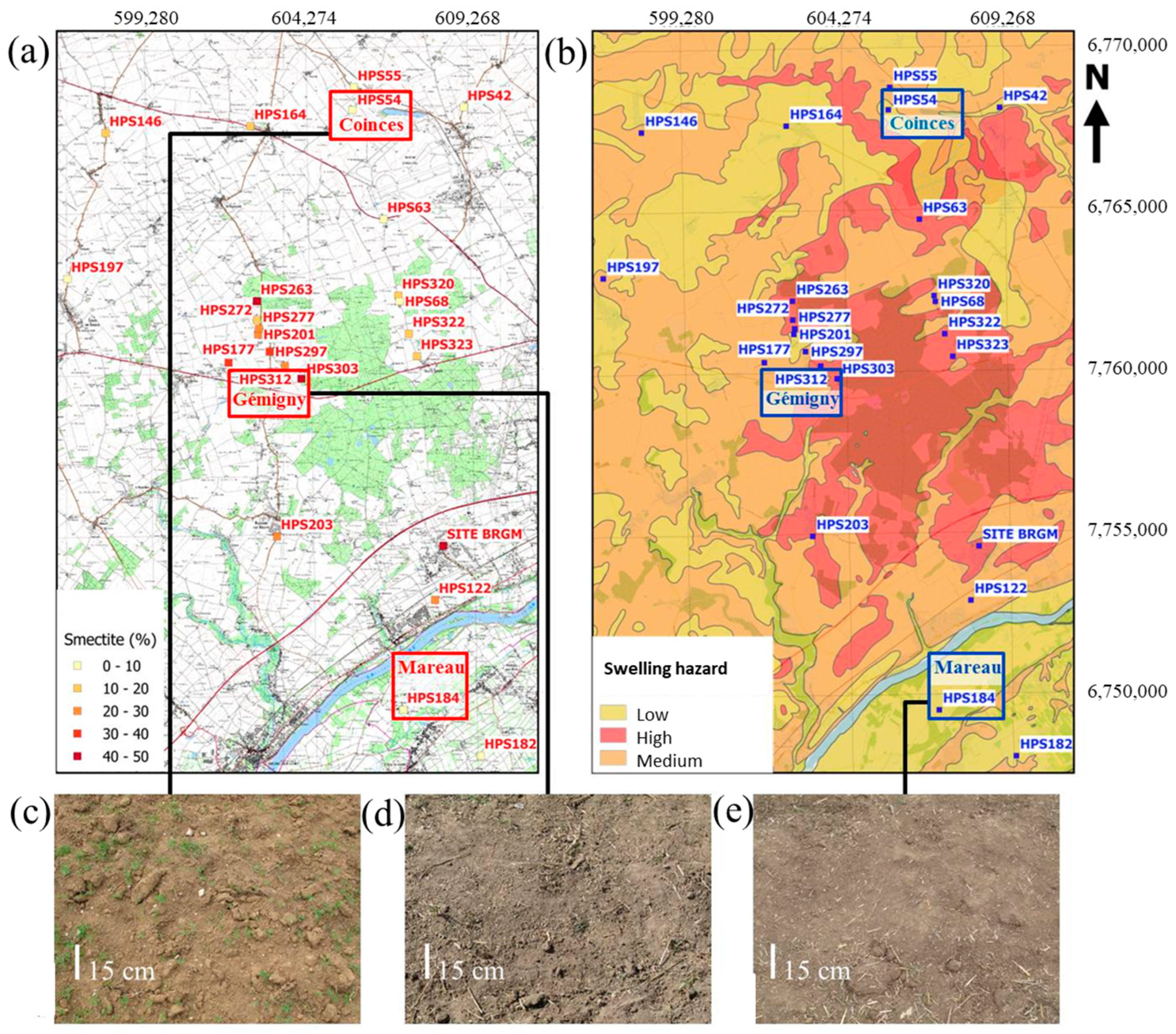
  • Soil swelling hazard maps from the BRGM [8] (Figure 1b) were used to roughly locate the previous XRD measurements. Their three classes (low/medium/high swelling classes) were selected using geotechnical analysis (MBT) and dominant lithology inside stratigraphic formations. The sites were chosen within the swelling class entity where the XRD measurements were sampled.
• An easy access to the selected sites given the field owner agreement.
• A low vegetation cover (less than 20%) observed on agricultural fields (the experiment has been carried out after wheat harvest, on freshly ploughed fields) (Figure 1c–e).

Thus, three sites among the available ones have been selected:

• “Le Buisson” locality in Coinces municipality, hereafter named Coinces (WGS 84, 48.00901°N, 1.734826°E). This site lies on a stratigraphic formation of Quaternary loam and loess, clayey and carbonated. The nearest XRD measurements indicate a composition of 11% kaolinite, 7% illite and 2% smectite, presenting a low swelling risk (Figure 1c).
• “Les Laps” locality in Gémigny municipality, hereafter named Gémigny (WGS 84, 47.95422°N, 1.689848°E). This site lies on a stratigraphic formation lower Pliocene sand and clay with dominant sand and clayey sand with metric clay layers. The nearest XRD measurement indicates 2.9% kaolinite, 5% illite and 43.5% smectite, presenting a high swelling risk (Figure 1d).
• “La Malandière” locality in Mareau-aux-près municipality, hereafter named “Mareau” (WGS 84, 47.83964°N, 1.758915°E). This site lies on a stratigraphic formation of recent Holocene Loire alluvium, mainly siliceous with local imbrications of loam and clay deposits. The nearest XRD measurements indicate 14.6% kaolinite, 6.5% illite and 0% smectite, presenting a low swelling risk (Figure 1e).

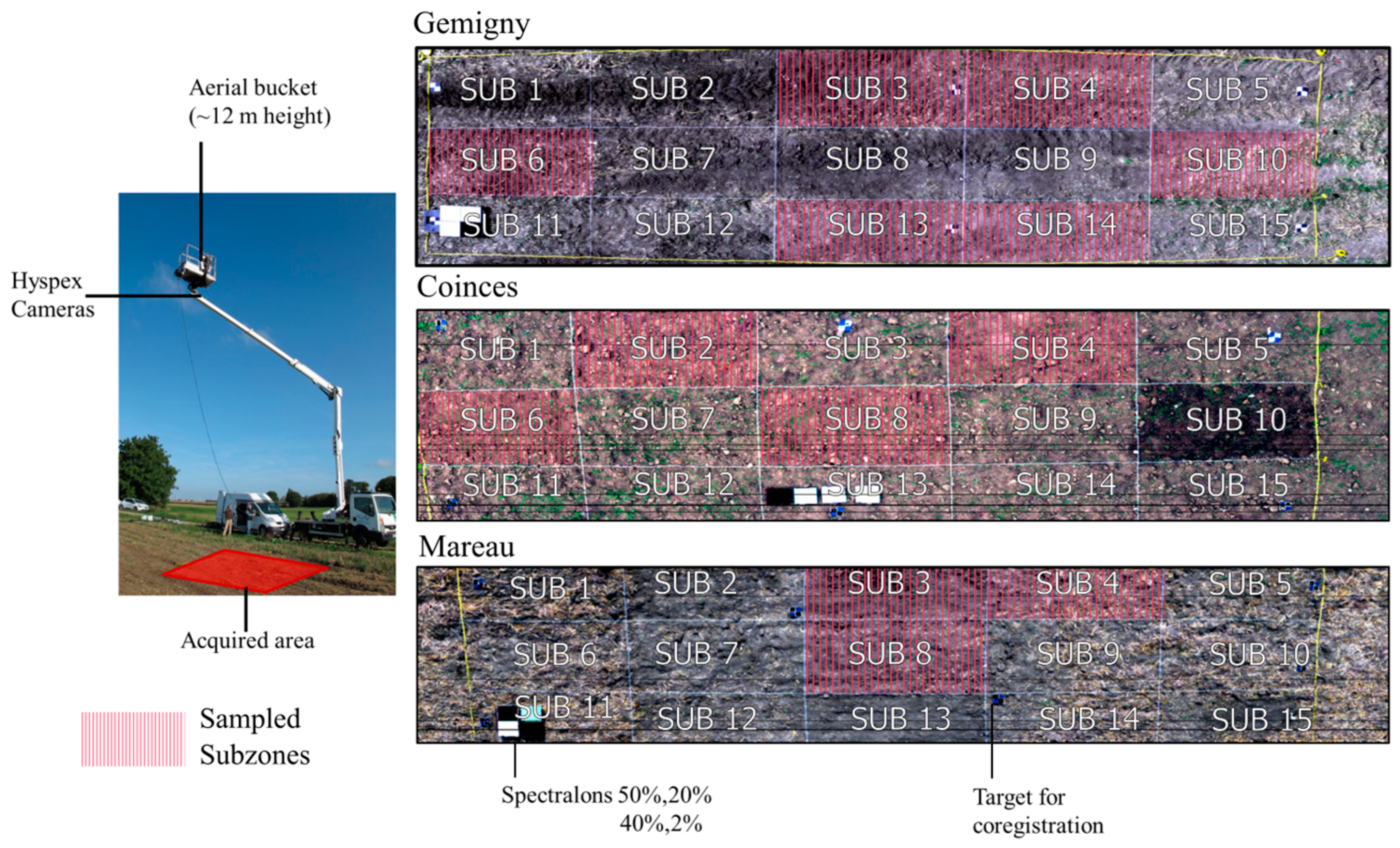
2.2. Hyperspectral Data Acquisitions

The outdoor experiment was performed between 5 and 7 September 2017 with hyperspectral cameras installed on a bucket truck at a height of 12 m (Figure 2). Two hyperspectral cameras (HySpex-NorskElektroOptikk–Visible Near-Infrared VNIR-1600-e and HySpex-NorskElektroOptikk-SWIR-320m-e) (HySpex, Oslo, Norway) acquired the reflected signal, with, respectively, 160 and 256 spectral bands with a spectral resolution of 3.6 nm for the VNIR camera and 6 nm for the SWIR camera. The two cameras covered a spectral range from 0.4 to 2.5 µm. The VNIR camera had a field of view (FOV) of 17°, and the SWIR camera had a FOV of 13.5°, leading to a spatial resolution at Nadir of, respectively, 0.4 cm and 1.5 cm. A rotating system made it possible to cover an area of 12 × 3.7 m² approximatively. The experimental area was divided into 15 rectangular areas of 2.4 × 1.3 m², or “subzones”, (called after as “SUB”). The acquisition setup was installed on each site for one day, in order to acquire several hyperspectral images at different periods along the day. However, due to high cloud cover and camera availability, only one image with the best illumination has been selected for each site. Gémigny (acquisition on September 6, local time: 11:20 a.m., solar elevation angle: 44°, sun azimuth angle: 147°) and Mareau (acquisition on September 7, local time: 3:13 p.m., solar elevation angle: 38.2°, sun azimuth angle: 227°) have been recorded with ideal weather condition. For Coinces, cloud cover was present all day, resulting in lower luminance measurements than the other sites (acquisition on September 5, local time: 3:48 p.m., solar elevation angle: 35.6°, sun azimuth angle: 235°). Signal-to-Noise Ratio (SNR) was obtained from the radiance images of the three test sites from a known reference panel (Spectralon^® 20%, Labsphere, North Sutton, NH, USA) present in the scenes. Coinces had a mean SNR in the SWIR domain of 29, and Gemigny and Mareau had a higher mean SNR of 58 and 49, respectively.

The acquired radiance images were then preprocessed. First, VNIR and SWIR images were coregistrated using Gefolki algorithm [51,52] with the SWIR image taken as the reference, leading to a coregistration RMSE less than the SWIR spatial resolution based on 30 random ground control points. Secondly, the conversion from radiance unit to reflectance one was performed using the empirical line method (ELM) with four calibrated known-reflectance targets (2%, 20%, 40%, 50% reflectance, Spectralon^® Labsphere, US, Diffuse Reflectance Targets, see Figure 2) placed in the scene [53,54]. These target values have been chosen to match the reflectance levels expected in the field. The luminance data corresponding to each spectralon were retrieved using a square-shaped ROI (size: 144 pixels) manually centered on each target. An average spectrum corresponding to the pixel average was extracted for each target. Inversion was performed over the entire image for each wavelength. ELM retrieved reflectance with an average 5% RMSE and r² of 0.94 on all wavelengths. Thirdly, strong atmospheric gaseous absorption spectral intervals were removed from the spectra: 747 nm–766 nm for O₂, 905 nm–1019 nm, 1094 nm–1176 nm, 1339 nm–1465 nm and 1773 nm–2005 nm for H₂O. Finally, 306 bands were kept over the original 416 bands. Fourthly, the minimum noise fraction (MNF) transform [55] was applied to remove the noise [21,22,56,57], and the first 20 eigenvalues bands were selected for the spectral reconstruction of VNIR and SWIR data. At the end, 54 spectral bands from the SWIR (2100–2425 nm) were used to discriminate clay minerals, and the VNIR bands were used for masking the presence of shadow and dry/green vegetation.

For shadow masking, the Nagao index image (or intensity image) was computed based on [58]:

$$I={\displaystyle \frac{2\times \left({\rho }_{1000}+{\rho }_{650}\right)+{\rho }_{475}+{\rho }_{550}}{6}}$$

(1)

With ${\rho }_i$ the reflectance of image pixel at $i$ nm ($i$ = 1000, 650, 475 and 550). An arbitrary threshold has been manually fixed to 0.075 to discard shadowed pixels [59].

For vegetation masking, two vegetation spectral indices were combined:

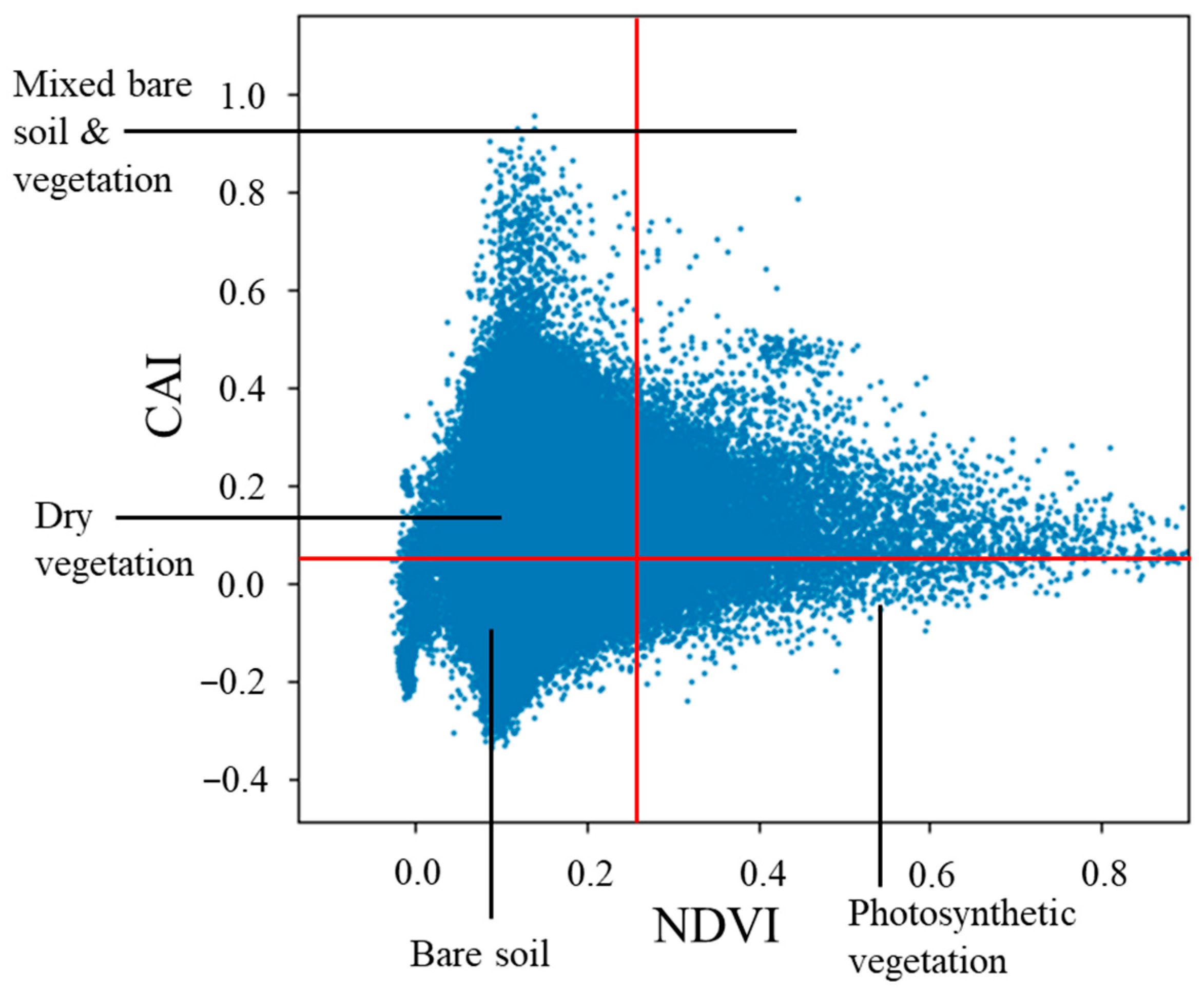
• Normalized difference vegetation index (NDVI) to detect green vegetation [60]:

$$NDVI={\displaystyle \frac{{\rho }_{810}-{\rho }_{680}}{{\rho }_{810}+{\rho }_{680}}}$$

(2)

• Chlorophyll absorption index (CAI) to detect dry vegetation [61]:

$$CAI=\left(0.5\times \left({\rho }_{2000}-{\rho }_{2100}\right)-{\rho }_{475}\right)\times 10$$

(3)

In the CAI-NDVI space, pixels were classed as bare soils when NDVI < 0.25 and CAI < 0.03 (Figure 3). These thresholds have been empirically defined from the image. Hereafter, only bare soil pixels were processed.

2.3. Field and Laboratory Measurements

Digital photos were acquired several minutes prior to the hyperspectral acquisition from a telescopic pole in order to build a digital elevation model (DEM) with MicMac software (version 1.0.beta13) [62] at a resolution of 1.3 mm, resampled to the hyperspectral images’ resolution. Hilllshades maps were then obtained using Geographic Information System software (QGIS, version 2.18) from the DEM, using the illumination parameters (solar elevation and azimuth) for each scene. The resulting maps were then normalized in percent in order to model a level of illumination of the scene, designated as a roughness index.

Six samples have been collected post-acquisition of the hyperspectral images on the Gémigny field site (SUB 3, 4, 6, 10, 13 and 14), four on Coinces (SUB 2, 4, 6 and 8) and three on Mareau (SUB 3, 4 and 8) (Figure 2). The samples were taken on the surface of the overall subzone, allowing a single integrated measurement over the surface of the subzone.

Then, their mineral composition and abundance were quantitatively estimated in laboratory on the samples using XRD analysis [63] with a Bruker D8 °θ/°2θ diffractometer. The analysis was separated in two steps. First, the crystallized fraction of the samples was determined from the powder diffractogram (detection threshold inferior to 3%). Second, the oriented clay fraction (<2 µm) was analyzed after solvation with ethylene glycol and heating at 490 °C. Error could reach 5% for the clay minerals estimation. Mineralogy estimation was realized using the SiroQuant version 4 software and was based on the Rietvield method [64].

They had similar abundances of clay minerals, with smectite (containing montmorillonite) ranging between 13% and 23%, illite between 1% and 10% and kaolinite between 1% and 7%. Calcite was only present in the SUB 4 of the Coinces site, with an abundance of 7%. Quartz was present in high abundance for Gémigny and Coinces, accounting for more than 58%, while it was only around 30% for Mareau. The remaining part of soil mineral fraction for Mareau consisted mainly of potassium feldspars and plagioclases (

Table 1. Mineral XRD analysis of samples collected on the 3 sites (statistics over the subzones per site).

Title 1	Gémigny		Coinces		Mareau
Type of Mineral	Min	Max	Min	Max	Min	Max
Quartz	58	68	58	64	29	31
Smectite	13	20	18	23	17	20
Illite and/or micas	3	5	1	4	6	10
Kaolinite	1	5	2	3	5	7
Calcite	traces	traces	traces	7	traces	traces
Potassium Feldspars (Sanidine/Orthoclase)	9	10	5	7	12	16
Plagioclase Feldspars (Albite)	4	7	5	6	18	24
Quartz	58	68	58	64	29	31

). As they are spectrally inactive in the SWIR domain, they will be considered similar to the quartz in the current study.

Factors influencing the spectral behavior of soil such as SOC, soil granulometry (Figure 4) and SMC were analyzed on the same samples. Clay granulometry was similar for Mareau and Coinces (around 30%) and lower for Gémigny (around 23%). For Gémigny and Mareau, silt represented 25%, while silt represented more than 50% for Coinces. A high proportion of sand was found for Gémigny (around 64%) and Mareau (around 43%) compared to Coinces (around 15%). SOC varied between 2% and 3% whatever the site.

SMC was measured a few minutes prior the acquisition on two areas: samples outside the hyperspectral acquisitions and samples in subzones that were manually wet (SUB 10 for Coinces and SUB 15 for Mareau). After the samples were collected, the mass was measured on site; then, samples were dried at 38 °C in an autoclave for 72 h in laboratory and measured for dry mass. Soils in the three sites were quite dry, with an SMC ranging between 8 and 10 wt% for Gémigny, between 8 and 13 wt% for Mareau, and between 2 and 8 wt% for Coinces. For the wet subzones, SMC reached 17 wt% for Mareau and 18 wt% for Coinces.

2.4. General Methodology

The processing flowchart is detailed in Figure 5. The first step defined the EM used as inputs for unmixing methods. Two options were tested: (i) detection from the hyperspectral image itself with automatic methods (Section 2.4.1) and (ii) selection from a spectral library. Then, after the application of spectral preprocessing (Section 2.4.2), linear and nonlinear unmixing methods were applied (Section 2.4.3) to give abundance maps that were compared with ground measured data in Section 2.4.4.

2.4.1. Endmember Selection

On one side, if all minerals are known for a given soil sample, the EM will be chosen from a spectral library. In our study, two spectral libraries were tested and independently applied. The first one comes from the United States Geological Survey (USGS) with more than 1270 spectra [65] and is widely used by the soil community. We selected spectra from the purest sampled for each minerals, (i.e., 4 for montmorillonite, 4 for illite, 4 for kaolinite, 4 for quartz and 2 for calcite) and used the average spectra for each EM. The second one corresponds to pure samples of minerals acquired in a previous laboratory study [12], with the same sensor as the present study with XRD analysis. This dataset is composed of mixtures of montmorillonite, illite, kaolinite, quartz and calcite and is further named the Ducasse library. More than 25,000 spectra have been acquired per minerals, recording the spectral variability of these EM.

On the other side, if all minerals were unknown, an automatic EM detection was performed. Two geometric methods were selected considering no pure pixel existed in the image: minimum volume constrained non-negative matrix factorization (MVC-NMF; [66]) and simplex identification via split augmented Lagrangian (SISAL; [67]). They were both based on a simplex detection and supposed the number of EMs to be known. MVC-NMF differs from SISAL by its non-negativity constraint. Both methods were initialized with the vertex component analysis (VCA [68]), using 4 or 5 mineral spectra.

2.4.2. Spectral Preprocessings

We selected six spectral preprocessings commonly used by the soil scientific community and also in our previous laboratory study [12]: pseudo-absorbance (Log(1/R)), Hapke model, standard normal variate (SNV), continuum removal (CR), continuous wavelet transform (CWT) and first Savitzky–Golay derivative (1stSGD). The reflectance (no preprocessing) was also kept (REF) as input for the unmixing process. More details about their formulation are provided in [12] and were coded in Python.

2.4.3. Unmixing Methods

Four unmixing methods were applied since there were already used in [12]: fully constrained least square (FCLS) and multiple endmember spectral mixture analysis (MESMA) as linear methods, and generalized bilinear model (GBM) and multi-linear model (MLM) as nonlinear ones.

FCLS algorithm ([69]; Equation (4)) with $f_i$ corresponds to the abundance of EM$i$, $p$ the number of EM and ${\rho }_i$ the reflectance of EM$i$.

$$\rho =\sum _{i=1}^p\left(f_i{\rho }_i\right){ with 0\le f}_i\le 1 and \sum _{i=1}^p\left(f_i\right)=1$$

(4)

MESMA ([70]; Equation (5)) accounts for the spectral variability of each EM by adding a new factor ${\epsilon }_{\lambda k }$ that is the residual error, λ being the wavelength index. Therefore, for each EM, six spectra were considered: mean spectrum, mean spectrum ± standard deviation, mean spectrum ± 3 × standard deviation and median spectrum.

$$\begin{gathered} \rho =\sum _{i=1}^p\left(f_i{\rho }_i\right)+{\epsilon }_{\lambda }{ with 0\le f}_i\le 1 and \sum _{i=1}^p\left(f_i\right)=1 \\ \mathrm{and} RMS={\left({\displaystyle \frac{{{\sum }_{\lambda =1}^N\left({\epsilon }_{\lambda }\right)}^2}{N}}\right)}^{1/2} \end{gathered}$$

(5)

GBM ([71]; Equation (6)) takes into account first- and second-order interactions but does not consider self-interactions:

$$\rho =\sum _{i=1}^p\left(f_i{\rho }_i\right)+\sum _{i=1}^{p-1}\sum _{j=i+1}^p\left({\gamma }_{ij}{f}_i{f}_j{\rho }_i\odot {\rho }_j\right)$$

(6)

${\gamma }_{ij}$ is a free parameter corresponding to the nonlinear contribution where i (respectively, j) referred to the EMi (resp. EMj).

MLM ([72]; Equation (7)) considers the parameter $P$ corresponding to the probability for a ray light to undergo multiple interactions.

$$\rho ={\displaystyle \frac{(1-P){\sum }_{i=1}^p{f}_i{\rho }_i}{1-P{\sum }_{i=1}^p{f}_i{\rho }_i}}$$

(7)

The implementation of the FCLS algorithm comes from the pysptools Python’s package. We coded our own version of MESMA based on [70]. GBM and MLM matlab implementation from [71] were used.

2.4.4. Evaluation Criteria

Three criteria evaluated the performances of these models and are expressed in the percentage of weight abundances (wt%). These criteria were made on a difference between the single measured montmorillonite value per subzone (measured, i.e., the XRD measurements, Section 2.3) and the abundance values estimated by unmixing. The measured value is therefore a single value for the entire zone; this is the difference with this validation value.

The mean bias (MB) will evaluate the mean error between estimated abundance ${\widehat{f}}_n$ and the measured one $f_n$ for a pixel n among the $M$ pixels of each image region of interest (subzone) or the whole image:

$$MB={\displaystyle \frac{1}{M}}\left(\sum _{n=1}^M({{\widehat{f}}_n-f}_n )\right)$$

(8)

The standard deviation is expressed as:

$$STDB=\sqrt{{\displaystyle \frac{1}{M-1}}\left(\sum _{n=1}^M{\left(\right({{\widehat{f}}_n-f}_n )-MB)}^2\right)}$$

(9)

The Root Mean Square Error (RMSE) is:

$$RMSE=\sqrt{{MB}^2+{STDB}^2}$$

(10)

In addition, the RMSE and the spectral angle mapper (SAM, [73]) were used to compared spectral library spectra and hyperspectral image spectra. Let $R$ be a reference spectrum, $T$ be the test spectrum, with $B$ the number of spectral bands; SAM is expressed as:

$$SAM={\cos }^{-1}\left({\displaystyle \frac{\sum _{\lambda =1}^B{T}_{\lambda }{R}_{\lambda }}{\sqrt{\sum _{\lambda =1}^B{T}_{\lambda }} \sqrt{\sum _{\lambda =1}^B{R}_{\lambda }}}}\right)$$

(11)

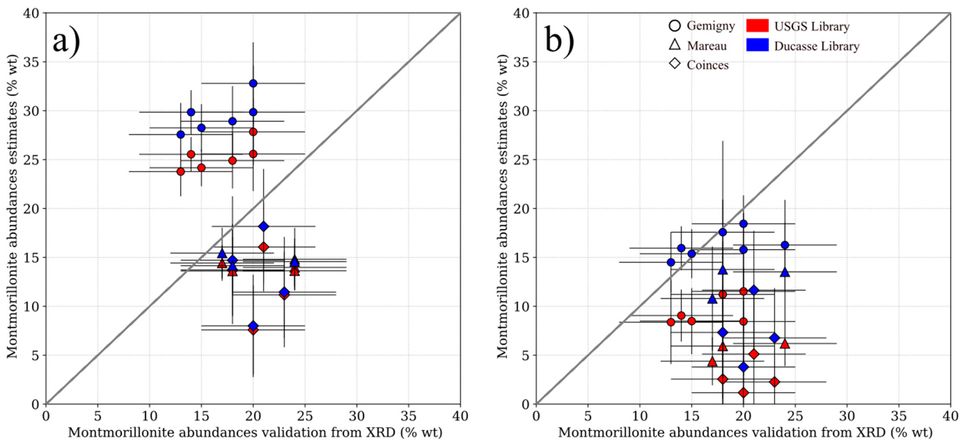
2.4.5. Validation Methodology

The validation was performed in three steps. First, spectra retrieved from automatic detection methods and from spectral libraries (USGS) were compared to the Ducasse library, visually and with the evaluation criteria (SAM and RMSE). Moreover, the position in the graph of mixtures is a good indicator of the accuracy of automatic detection methods.

Second, for the entire datasets, every preprocessing method coupled to unmixing methods, with different spectral libraries, was tested and presented. The evaluation criteria presented above (MB, STDB, RMSE) between XRD mineral composition of samples and estimated abundance values were used to choose the bests methods to retrieve montmorillonite abundances.

Then, the two best methods were compared at the subzone scale, then at the site scale, using visual interpretation.

3. Results

First, EM spectra derived from USGS and Ducasse libraries are compared with the results of the automatic EM detection (Section 3.1). Depending on this comparison, the best choice of EM spectra is further retained to be used with unmixing methods. Their performances are then described in three subsections: the montmorillonite estimates derived from all couples of spectral preprocessings and unmixing methods are compared to XRD smectite abundances as reference values (Section 3.2), the results for the best previous methodological couple are spatially interpreted over the three sites (Section 3.3), at subzone scale (Section 3.3.1) and image scale (Section 3.3.2), and the estimation of other soil minerals are compared with the best method (Section 3.4).

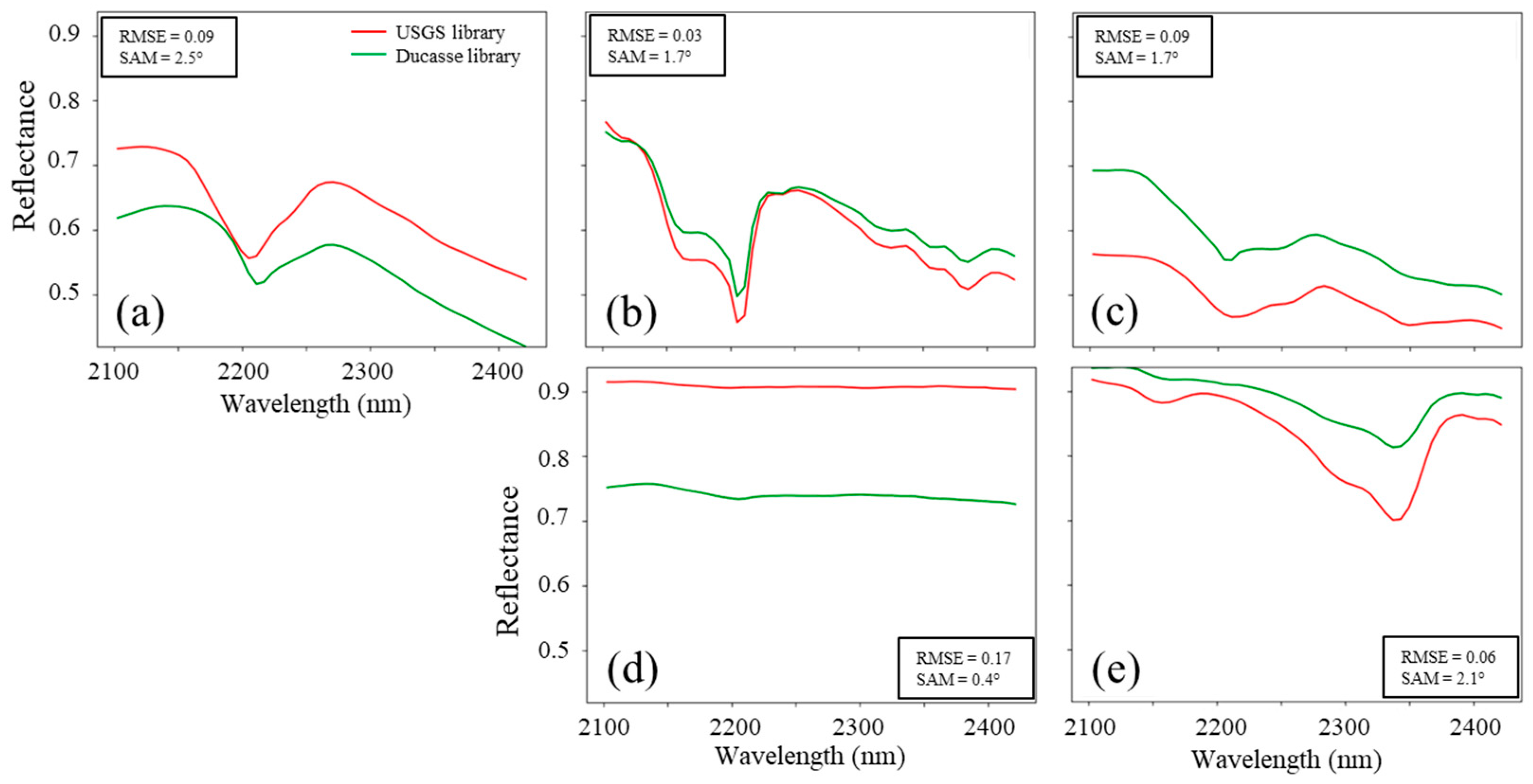
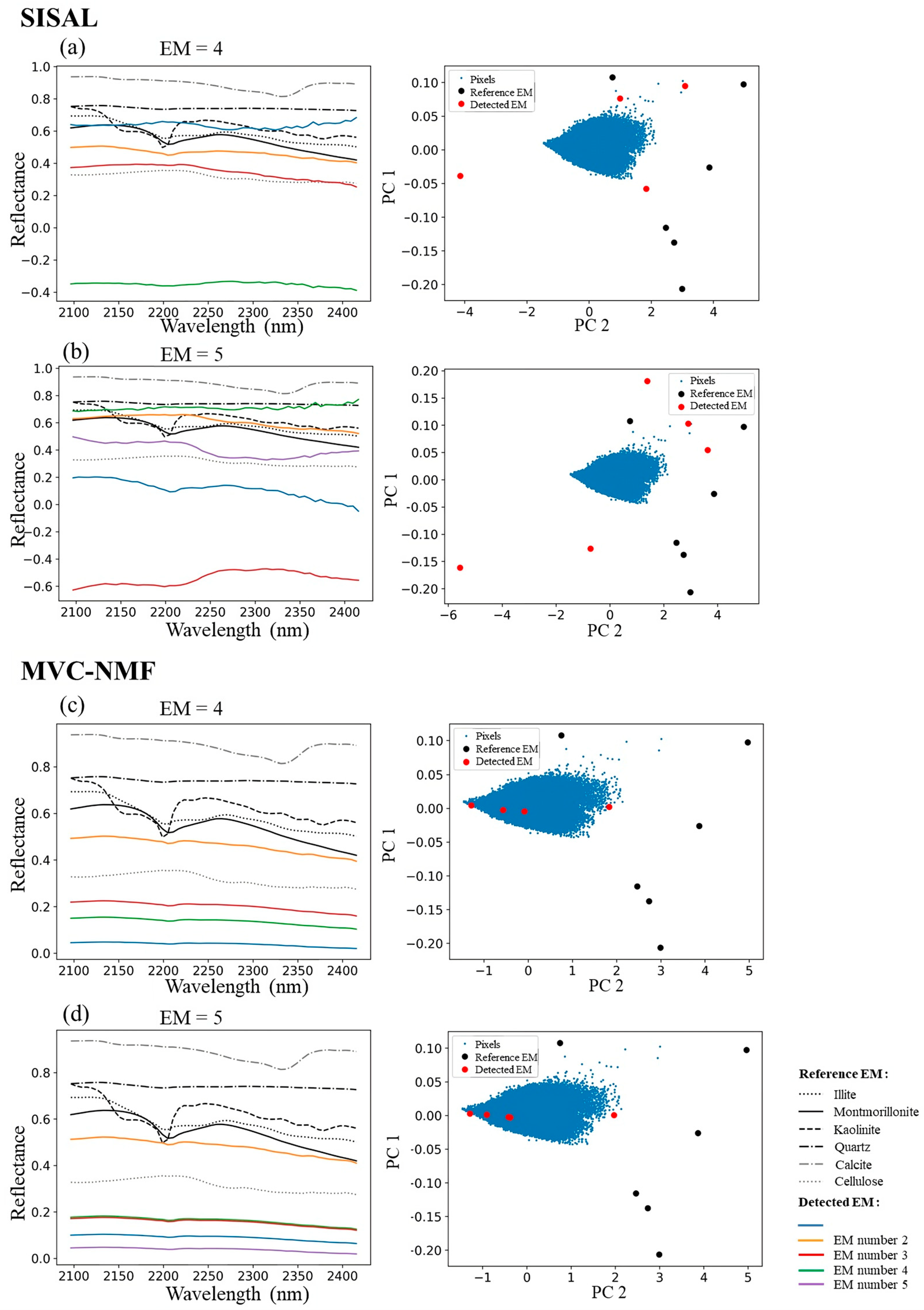
3.1. Endmember Detection and Comparison

USGS and Ducasse average spectra for every mineral were compared visually and then with SAM and RMSE (Figure 6). Generally, all mineral spectra presented the same spectral behavior (small SAM values) but differed in their absolute reflectance level (higher RMSE values). For montmorillonite, the SAM was less than 3°, and the spectral band at maximum absorption depth shifted by 10 nm (Figure 6a). For quartz, the RMSE was 17% with a SAM of 0.4°. The lowest RMSE (0.03%) was obtained for kaolinite. Calcite absorption features were deeper with the USGS library than with the Ducasse one.

The application of SISAL and MVC-NMF with VCA initialization showed similar results whatever the site; thus, only the results from Gémigny are shown (Figure 7). By applying SISAL with four or five EMs, the retrieved EMs did not exhibit specific clay or calcite absorption features (except slightly for EM2 and EM1 (Figure 7a,b, left). This was also confirmed by the fact that the detected spectra were outside the image simplex and far from the reference ones (Figure 7a,b, right) instead of being at the extremities of the simplex. MVC-NMF showed the worst results with all spectrally flat EMs whatever the initialization.

In conclusion, EM spectra were taken from the spectral libraries given the bad performances of the automatic EM detection methods.

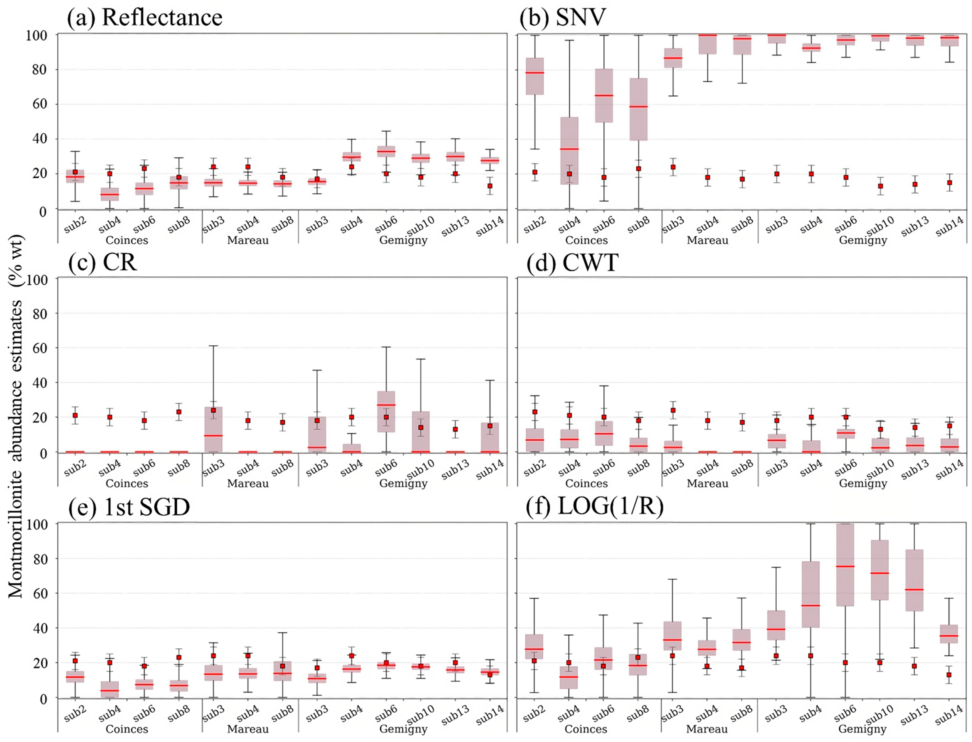
3.2. Performance Analysis of Spectral Preprocessing Coupled with Unmixing Methods for Montmorillonite Abundance Estimation

The montmorillonite abundance estimated with FCLS, MESMA and GBM had most values close to either 0% or 100%, whatever the spectral library and the spectral preprocessing. Although GBM is a nonlinear model, its nonlinear fraction γ equals 0, meaning that GBM behaves like a linear unmixing method as FCLS or MESMA.

With MLM and USGS library as input, the best performances were obtained with REF whatever the site (the range of predictions encompasses this of measurements), with an RMSE between 2.2% and 13.3% (

Table 2. Performances of Montmorillonite abundance estimations (wt%) obtained with REF-MLM and 1stSGD-MLM with the USGS library. In bold, the best RMSE, mean bias and standard deviation are presented for each sample.

	REF-MLM						1stSGD-MLM
Sample	Average Abundance	XRD Validation	MB	STDB	RMSE	R	Average Abundance	XRD Validation	MB	STDB	RMSE	R
Coinces sub2	15.6	21	−5.4	4.3	6.9		7.6	21	−13.4	6.6	14.9
Coinces sub4	7.4	20	−12.6	4.1	13.3		3.5	20	−16.5	5.1	17.3
Coinces sub6	13.2	18	−4.8	4.3	6.4		3.7	18	−14.3	3.3	14.7
Coinces sub8	10.5	23	−12.5	4.0	13.1		3.6	23	−19.4	3.5	19.7
Coinces all subs	12.8	21	−7.8	6	9.8	−0.08	4.3	21	−16.3	5.4	17.1	0.05
Gémigny sub3	27.8	20	7.8	3.4	8.5		12.2	20	−7.8	4.3	9.0
Gémigny sub4	25.0	18	7.0	2.9	7.5		12.3	18	−5.7	5.4	7.9
Gémigny sub6	25.5	20	5.5	3.8	6.6		9.5	20	−10.5	5.5	11.8
Gémigny sub10	23.9	13	10.9	2.5	11.1		9.3	13	−3.7	4.3	5.7
Gémigny sub13	25.5	14	11.5	1.8	11.7		9.5	−14	−4.5	2.7	5.3
Gémigny sub14	24.2	15	9.2	1.9	9.4		9.2	15	−5.8	3.4	6.7
Gémigny all subs	25.6	17	8.6	3.4	9.2	0.27	10.7	17	−6.4	4.6	7.9	0.23
Mareau sub3	13.7	24	−10.3	1.6	10.4		6.6	24	−17.4	2.3	17.6
Mareau sub4	13.6	18	−4.4	2.0	4.9		8.4	18	−9.6	8.4	12.7
Mareau sub8	14.5	17	−2.5	1.8	3.1		4.7	17	−12.3	2.5	12.5
Mareau all subs	14.0	20	−6.2	4.1	7.4	−0.17	6.0	20	−14.1	4.9	15.0	0.14
All subzones, all sites.	18.9	18	0.0	9.0	9.0	−0.44	18.9	−11.3	−11.3	6.7	13	−0.17

). It was also the case for Gémigny and 1stSGD on one side (RMSE between 1.4% and 11.8%) and for Coinces/Mareau and LOG(1/R) on another side (Figure 8 and Table 2). But the latter presented much higher prediction dispersions compared to Reflectance and 1stSGD. The results with theDucasse library were the same as the USGS library for REF (RMSE between 3% and 13%), better for 1stSGD (RMSE between 2.6% and 16.3%), particularly with Gémigny (2.6–5.4%), and a bit worse for LOG(1/R) (with higher prediction dispersions whatever the site) (Figure 9 and

Table 3. Performances of Montmorillonite abundance estimations (wt%) obtained with REF-MLM and 1stSGD-MLM with the Ducasse library. In bold, the best RMSE, mean bias and standard deviation are presented for each sample.

	REF-MLM						1stSGD-MLM
Sample	Average Abundance	XRD Validation	MB	STDB	RMSE	R	Average Abundance	XRD Validation	MB	STDB	RMSE	R
Coinces sub2	17.6	21	−3.4	5.9	6.8		12.3	21	−8.7	5.5	10.3
Coinces sub4	6.9	20	−13.1	4.7	14.0		6.2	20	−13.8	6.5	15.3
Coinces sub6	13.6	18	−4.4	6.3	7.6		7.9	18	−10.1	4.3	11.0
Coinces sub8	10.2	23	−12.8	5.3	13.8		7.4	23	−15.6	4.6	16.3
Coinces all subs	13.9	21	−6.6	7.4	9.9	−0.07	8.6	21	−12.0	6.4	13.6	0.05
Gémigny sub3	32.7	20	12.7	4.2	13.4		18.4	20	−1.6	2.9	3.3
Gémigny sub4	28.9	18	10.9	3.6	11.5		17.9	18	−0.1	3.3	3.3
Gémigny sub6	29.5	20	9.5	4.7	10.7		16.1	20	−3.9	3.7	5.4
Gémigny sub10	27.7	13	14.7	3.2	15.0		15.0	13	2.0	3.1	3.7
Gémigny sub13	29.8	14	15.8	2.2	16.0		16.1	14	2.1	2.2	3.0
Gémigny sub14	28.3	15	13.3	2.4	13.5		15.5	15	0.5	2.5	2.6
Gémigny all subs	29.9	17	12.8	4.00	13.4	0.26	16.9	17.1	−0.2	3.4	3.4	0.29
Mareau sub3	14.6	24	−9.4	2.4	9.7		14.3	24	−9.7	5.0	10.9
Mareau sub4	14.1	18	−3.9	2.9	4.9		17.3	18	−0.7	13.2	13.2
Mareau sub8	15.5	17	−1.5	2.6	3.0		11.5	17	−5.5	5.3	7.6
Mareau all subs	14.9	20	−5.3	4.5	6.9	−0.11	14.9	20	−6.7	7.3	10.1	0.12
All subzones, all sites.	21.4	19	2.5	10.8	11.1	−0.43	13.6	19	−5.3	7.6	9.3	−0.17

). Then, whatever the spectral library, SNV, CR and CWT led globally to poor estimations, all roughly close to either 0% or 100%.

The best preprocessing–unmixing methods (i.e., 1stSGD-MLM and REF-MLM), compared to our validation dataset, give a negative r value for both methods, with a more pronounced negative trend (−0.44) for REF-MLM, due to montmorillonite overestimation for the Gemigny site (Figure 10a) and underestimation for Coinces and Mareau. Using different spectral libraries gave the same results (Figure 10). Noticeable trends were visible for Gemigny, with an r value between 0.23 and 0.29 for both methods and spectral libraries. This result suggests that unmixing could estimate montmorillonite abundances variations closely on this site.

By considering the different assessment metrics in Table 2 and Table 3 and Figure 10, it remains difficult to evaluate which spectral library is the best choice. Plus, as presented above (Figure 6), the libraries are very similar. Thus, USGS library was further chosen because it is a worldwide reference database for the soil community. In the following, only 1stSGD-MLM and REF-MLM were studied.

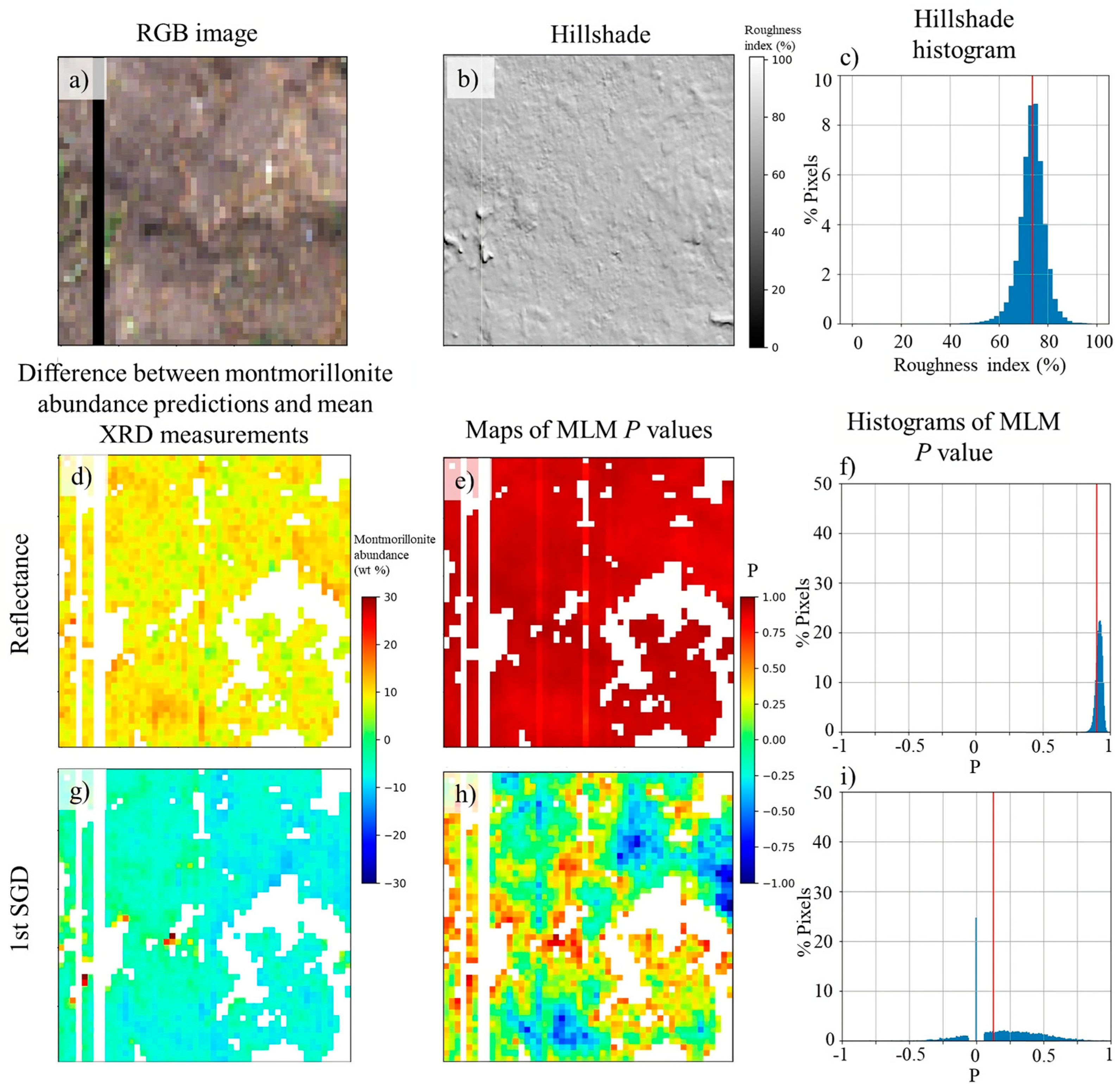
3.3. Analysis of Montmorillonite Abundance Maps

3.3.1. At the Subzone Scale

In order to understand the combined impact of topography (through the roughness index) and illumination conditions (through the solar elevation angle) on montmorillonite spatial estimation, two extrema subzone cases were selected among the three sites:

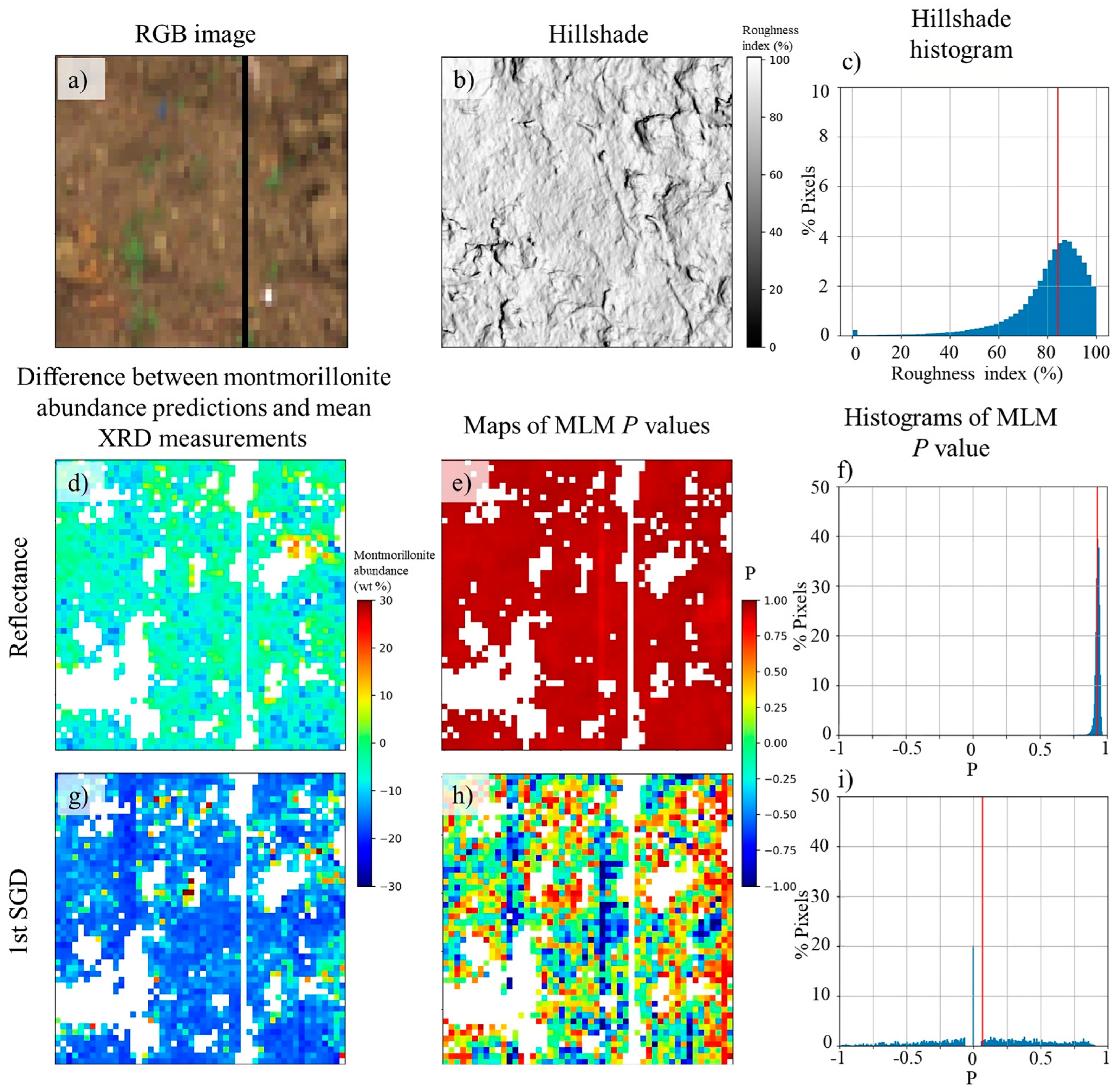
• Gémigny-SUB14, characterized by a weak spatial variability of the roughness index (median and standard deviation of 0.51 cm and 0.68 cm (Figure 11c) and by a solar elevation angle of 44°.
• Coinces-SUB2, characterized by a large spatial variability of the roughness index (median and standard deviation of 83% and 0.51 cm and 0.68 cm (Figure 12c), and a solar elevation angle of 35.6°.

In addition, the nonlinearity of MLM was analyzed by studying the variability of the parameter $P$.

For REF-MLM, the montmorillonite abundance estimations were rather spatially homogeneous for Gémigny-SUB14 with a spatial STDB of 1.9% (Figure 11d), but more heterogeneous for Coinces-SUB2 with 6.9% (Figure 12d). However, abundance values were overestimated for Gémigny-SUB14 (MB of 9.2%) and underestimated for Coinces-SUB2 (MB of −5.2%). Whatever the subzone, the p-value maps were very homogeneous (Figure 11e and Figure 12e), leading to narrow distributions ranging between 0.75 and 1 (Figure 11f and Figure 12f).

For 1stSGD-MLM, abundance estimations also had little variations on Gémigny-SUB14, with a spatial STDB of 3.4% (Figure 11g), while for Coinces-SUB2, they presented more variability with 6.6% (Figure 12g). Abundance values were underestimated for Gémigny-SUB14 (MB of −5.8%) and much more for Coinces-SUB2 (MB of −13.4%). The p-value range was larger with 1stSGD-MLM than with REF-MLM with negative values (between −0.4 and 0.6) (Figure 11f,i).

Globally, 1stSGD-MLM tended to estimate negative values of montmorillonite abundances, which was more marginal for REF-MLM. Therefore, for its simplicity, REF-MLM was selected to map the entire sites.

3.3.2. At the Image Scale

For Coinces, the average abundance of montmorillonite over the image was 15%, whereas XRD data were between 18% and 23% over the subzones (Figure 13a). The montmorillonite abundance was underestimated on all subzones, particularly on SUB4 and SUB8 (respectively, 7% and 10%). The subzone interquartile range (around 5%) was larger than that of the entire image (7%).

For Gémigny, the average abundance of montmorillonite was between 24% and 28% for all subzones and 23% for the entire image (Figure 13b). In comparison, XRD data ranged between 13% and 20% for this site. Interquartile ranges were around 5% for all boxplots.

For Mareau, the average abundance of montmorillonite was between 14% and 15% for all subzones and 14% for the entire image (Figure 13c). In comparison, XRD data ranged between 17% and 24%. Interquartile ranges were around 3% for all boxplots. It seems that fewer outliers were observed for Mareau than for the other sites at the image scale, and also the montmorillonite abundance was globally underestimated with Coinces and Mareau, opposite to Gémigny.

On the three montmorillonite abundance maps, the estimates were spatially uniform (Figure 14, Figure 15 and Figure 16). We can note:

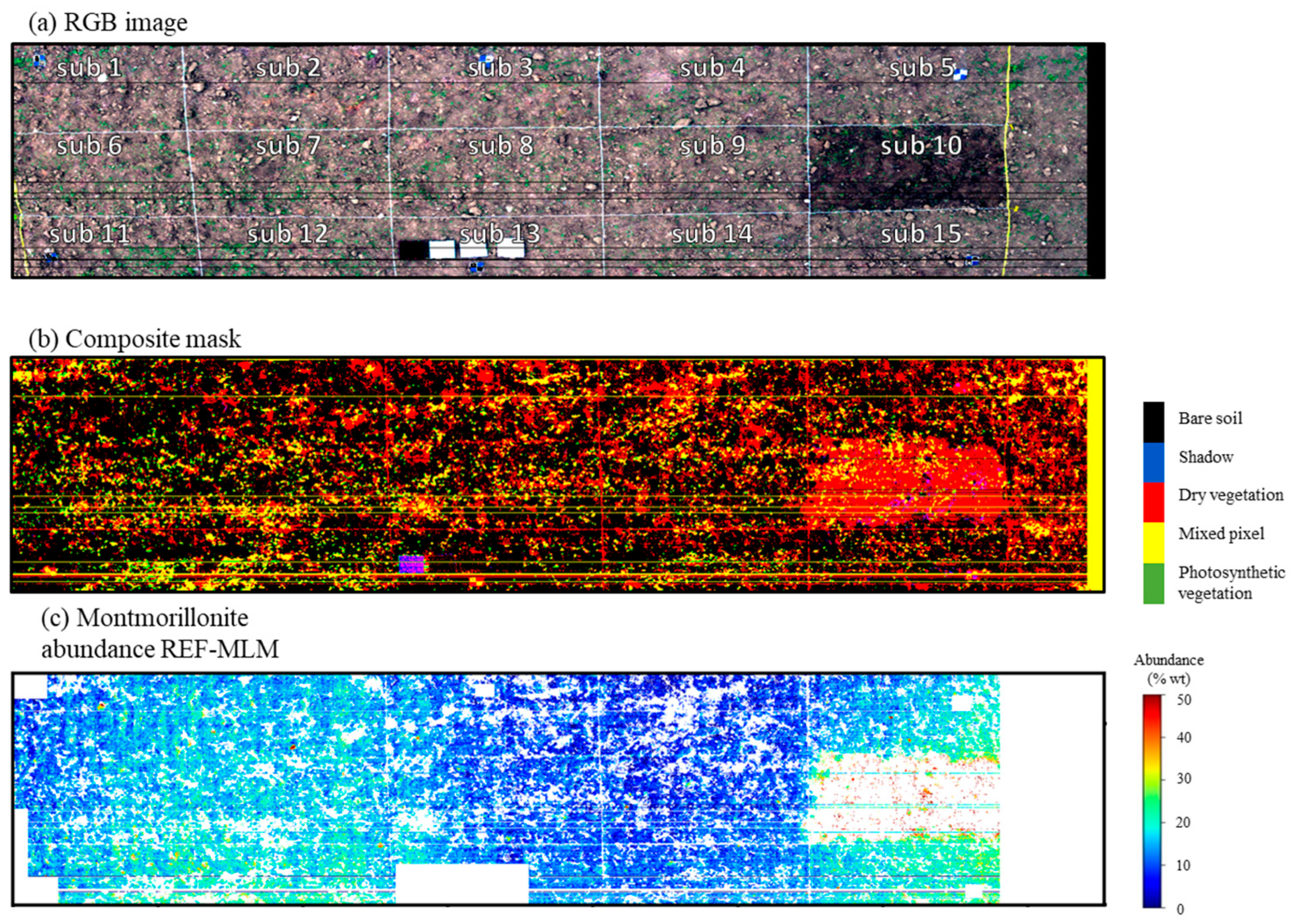
• On the Gémigny map, the estimated abundance values of clays increased inside wheel tracks located in SUB1, SUB2, SUB3, SUB7, SUB8 and SUB9 (Figure 14c). They contained more estimated montmorillonite than the other subzones (from around 4% to 5%).
• On the Coinces map (Figure 15c), the montmorillonite estimation was higher in left subzones (SUB1, SUB2, SUB6, SUB7, SUB11, SUB12) than in the right ones (SUB5 and SUB15). This trend was not present in any validation data but may have been due to the presence of clouds during the acquisitions. In the wet subzone (SUB10), the majority of pixels was wrongly classified as “dry vegetation”, and montmorillonite was estimated at around 40% in bare soils’ pixels.
• On the Mareau map, the montmorillonite estimation was around 20% in the wet subzone (SUB15), whereas the montmorillonite estimation in other pixels was around 15% (Figure 16c).

The composite mask showed that only 53.6%, 59.2% and 42% of the image was composed of bare soil, respectively, for Gémigny, Coinces and Mareau. The main contribution in the masks came from dry vegetation, while the rate of mixed pixels was relatively low, except for Coinces (cf. Figure 14, Figure 15 and Figure 16).

3.4. Estimation Performances of Other Mineral Abundance

As the estimation quality of montmorillonite abundance depends on that of the other minerals composing the soil, there is an interest to study it. Our results were close for all sites due to the soil composition uniformity (Figure 17a–c). Best performances for mineral estimation were obtained for kaolinite (RMSE between 1% and 7%). Quartz was estimated with the largest errors (RMSE range between 8% and 22%). Illite estimation for REF-MLM was equal to zero for Mareau and Gémigny, whereas there was between 6% and 10% illite in Mareau soil and between 2% and 5% illite in Gémigny soil (Figure 17b,c). Calcite mineral was estimated with low errors (RMSE range between 4% and 6%); however, this mineral has been detected in only one subzone (SUB4 for Coinces site). These previous RMSEs were computed for all sampled subplots of an image.

4. Discussion

4.1. Endmembers Selection for Unmixing

Considering the automated EM selection methods, the detected EMs with MVC or SISAL methods presented a low spectral behavior, explaining why they failed to detect the correct EMs (Figure 7) [34]. In our study, the detected EMs were far from the extremities of the simplex and also from the EMs of the libraries. Further, these methods were very sensitive to the initialization achieved here with VCA. Depending on the prior number of EMs, the likelihood of estimated EM highly differed, particularly with SISAL. In addition, one could expect better results if these methods were initialized with prior knowledge of the minerals present in the sampled soils. Unfortunately, this was not the case here; one reason could come from the high spatial intra-class variability of each mineral in the image. In this work, it was the first time that automatic endmember selection methods were used for clay mineral abundance estimation over a real rough soil at a centimeter scale. The derived results were mitigated. This work was a first attempt at using simple tools; thus, more sophisticated tools could be tested accounting for the intra-class variability, such as the inertia-constrained pixel-by-pixel nonnegative matrix factorization [74] or the genetic algorithm [75].

Considering the choice of EMs from a spectral library, the unmixing performances were sensitive to the upscaling from laboratory spectroscopic measurements to real case scenarios, since USGS and Ducasse libraries did not come directly from the study sites. Nevertheless, montmorillonite abundance estimations were rather coherent with the XRD measurements, and similar performances were obtained whatever the spectral library, suggesting that the leading factor was the spectral signature of minerals whatever the sampling site (cf. Figure 6, Table 2 and Table 3). For the five studied minerals, the SAM was globally below 2.9°, while in the literature, standard threshold values were most often higher. For instance, ref. [76] discriminated two mineral spectra on average with an SAM equal to 5.7°, and ref. [77] discriminated two clay spectra in the SWIR domain with 3.7°. Recently, ref. [78] developed an open synthetic dataset for the unmixing of 325 intimate mixtures from five clay powders. Overall, most available spectral libraries have focused on clay texture from the centimetric scale [79,80] to the global scale [81]. But, to our knowledge, except the two libraries we used, none of them have provided spectra associated with clay mineral discrimination, including montmorillonite.

4.2. Limitations of Preprocessings and Unmixing Methods for Montmorillonite Abundance Estimation

Considering the spectral preprocessings, they can be divided into three main classes [12]: those suppressing the spectral continuum and working at a local scale such as CWT and 1stSGD, those normalizing the global spectrum level such as SNV and CR and, at last those, that do not reduce the soil spatial variability such as Hapke and Log(1/R). Dealing with outdoor conditions in our case with the example of the MLM unmixing method (cf. Figure 8 and Figure 9), SNV, CR and CWT globally had very poor montmorillonite estimations (roughly close to either 0% or 100%) whatever the spectral library. SNV was very sensitive to the high spectral and spatial variabilities of field soils, which might explain the difficulty of the unmixing methods to converge because SNV is the ratio between the spectral deviation compared to the mean over the standard deviation. For CR, an important reduction of clay absorption features was induced from the high proportion of quartz in soil, which modified their shape (depth and width), leading to difficulties for unmixing methods to find the proper EMs. For CWT, the main limitations came from the linear wavelet base decomposition of the spectra accounting only for the second to the fifth order (the first order corresponding to noise), which was probably not enough sufficient to model the nonlinearity due to multiple scatterings. Log(1/R) projects the spectral reflectance in a logarithmic space, allowing an increase of the linearity between the spectral data and their abundance [82,83]. But this transform remains very sensitive to the high spatial variability, leading to a strong overlap between the intra- and inter-classes. The W single scattering albedo of Hapke is the fraction of photons scattered by a particle over the total fraction of photons affected by this particle. This model considered the soil as a homogeneous mixture with the same granulometry for all the constituents composing this soil. Unfortunately, our ploughed soil was very heterogeneous with different granulometries (Figure 4) that explain the poor results obtained for linear unmixing methods. The best preprocessing was 1stSGD, with similar results as REF. This is in agreement with [12] noting that the best one was also 1stSGD for clay mixtures and reflectance when other minerals than clay were added. Ref. [84] found among several preprocessings, including SNV, that the best was first Log(1/R) combined with 1stSGD.

Considering the unmixing methods, FCLS, MESMA and GBM failed to estimate montmorillonite abundance. The main limitation for GBM is that it is not able to account for the complete nonlinear contribution of the signal with just second-order interactions between any two EMs, and it finally behaves as an FCLS (cf. Equation (6)). In the laboratory, similar results were obtained with clay and clay–calcite mixtures [12]. Also, GBM does not consider self-interactions and has no restriction on reflectance values that could be out of the [0–1] physical range [71]. On the contrary, MLM was the only unmixing method delivering correct results by accounting for all the multiple interactions found for ploughed fields. On contrary, in laboratory conditions, both linear and nonlinear unmixing methods have globally provided similar performances for montmorillonite abundance estimation [12].

Deeper explanations on MLM performances and p value analysis are further discussed. Initially, MLM takes as inputs albedos instead of reflectance spectra. The authors of [72] mentioned that they can be assumed to be equivalent for remote sensing imagery with a spatial resolution of 20 m or 2.4 m where nonlinear effects are relatively small (leading to small p values). But albedos should be preferred in cases of intimate mixtures due to a larger number of interactions (p values close to one), if EM spectra are known. However, for the latter case in laboratory conditions, [72] showed good results by only using reflectance for quartz abundance estimation, the same as [12] for montmorillonite. The trade-off most often relies on the $P$ parameter of MLM having a physical meaning when its values are inside the range [0–1]. It indicates the probability that a light ray will undergo further reflections after each interaction and can thus be used to assess the size of the nonlinearity effect or the size of the deviation from a linear unmixing method. However, negative p values can occur if at least one material has a strong reflective behavior and/or a reflectance-albedo conversion has not been performed. Therefore, the observed spectra are larger in magnitude than any convex linear combination of EM spectra (given the same knowledge of EMs and abundances), and it is the opposite if the p values are positive [72]. Consequently, the analysis of p values is not straightforward, and very few studies have actually provided information about their distribution. In laboratory conditions, [12] found p values ranging [−0.2; 0.2] for montmorillonite–kaolinite mixtures and [−2; 0] for montmorillonite–calcite mixtures, while [72] found p values of 0.6, 0.71 and 0.88 for quartz–alunite mixtures. It seems that the presence of either quartz or calcite as reflective materials leads $P$ to its lowest or highest values. From airborne hyperspectral data at varying spatial resolutions (2.4, 5.2 and 20 m) over desert, heathland and seashore areas, [72] found p value distribution with ranges of [−1.4; 0.6], [−1.2; 0.8] and [−2.5; 0.5], respectively. The areas with strongest nonlinear effects are highlighted by the pixels’ highest $P$ absolute values (ex: road, shadow, tree and coastline), and pixels’ negative p values can come from additional illuminations due to adjacent topography outside the pixel field of view. Also, at coarse spatial resolutions, the unmixing problem is more due to areal mixtures than intimate ones. In our case, at the centimeter scale, both mixture types were encountered. Whatever the surface roughness, p values with reflectance exhibited a very narrow Gaussian distribution with a mean of 0.9 (Figure 11c and Figure 12c) and were spatially homogeneous (Figure 11e and Figure 12e). It might be attributed to the highest influence of the multiple scatterings from the predominance of intimate mixture effect and the quartz contribution in soils. It can also be attributed to the compensation between the high reflectance levels of the spectral library ranging from 50% up to 90% and those of the fields from 10 to 35%. A different behavior was observed when using 1stSGD instead of REF, which seems to be more sensitive to the topography and the surface composition, as if areal mixtures impacted more than intimate ones. This can be explained because reflectance bears the spectral continuum (and associated strong multiple scattering influence) oppositely to 1stSGD, which removes it (depends on local scale influences). For 1stSGD, p value distributions followed a very large Gaussian distribution over the range [−1; 1], with a majority of positive values for the less rugged terrain in comparison with the most rugged one having more disperse negative and positive p values (Figure 11i and Figure 12i). These distributions appear similar to those found at an airborne scale in [72]. Highest p values were mostly located around masked areas (Figure 11h and Figure 12h). Indeed, artefacts can remain from the masking operation (based on empirical thresholds) because properly unmixing with spectral indices the presence of shade, vegetation and bare soil can result in a hard task. MLM can compensate the absence of EMs for shade and vegetation by varying the p value. This phenomenon has been observed at a larger scale, for instance, for improving unmixing in tree shadow pixels [72]. Although MLM was developed to be applied on reflectance, the performances obtained with 1stSGD preprocessing were similar that those with REF (RMSE of 11.6% with 1stSGD-MLM and 12.7% with REF-MLM).

In the recent years, several works have proposed some improvements of MLM, like [85], by exploiting the underlying manifold structure of the pixels’ spectra; [86], by simulate the physics process of MLM with neural networks; [87], by proposing a coarse-to-fine scheme for unsupervised unmixing; and [88], by extending MLM to take into account multiple reflexions in the rough surface and different sources of illumination. Unfortunately, these extensions have only been validated either on synthetic datasets either on remote sensing data at least at a meter scale.

Other methods exist to retrieve the EMs and quantify their abundances. A large community has used linear based methods like PLSR, which are not adapted for complex soils (rough surface, intimate mixture, large variety of grain size) [72]. Recently, ref. [89] proposed another approach combining Fisher transformation and multiple endmember spectral mixture analysis to estimate lunar mineral abundance using the RELAB database. This method can address both the intra-class and inter-class variability of the spectral features of different lunar minerals and might be interesting to test on our dataset.

The best coupling preprocessing and unmixing methods are REF-MLM and 1stSGD-MLM. With laboratory clay mineral mixtures, best performances are obtained with 1stSGD-FCLS [12]. Indeed, intra-class variability has a higher amplitude than nonlinear effects in these mixtures, and derivative spectral preprocessing is the most efficient method to decrease intra-class variability. Using 1stSGD-FCLS, montmorillonite was estimated in mixtures of illite–montmorillonite–kaolinite with 10.8% RMSE, montmorillonite–calcite with 22.6% and montmorillonite–quartz with 55.2%. When upscaling to field conditions with more complex soil mineral composition, REF-MLM and 1stSGD-MLM methods provided RMSE performances within 2.2–13.3% and 1.4–19.7%, respectively, for REF-MLM and 1stSGD-MLM. The authors of [7] found an RMSE of 15.8% for fine fraction of soil samples coming from agricultural field using CR and a geometrical method trained with empirical relationships from synthetic laboratory mixtures. Ref. [90] estimated the abundance of smectite present in 77 samples collected in the Northern Morocco, with an RMSE of 18 wt%. After a CR, a multi-Gaussian method was applied on the resulting spectrum followed by a regression tree analysis to retrieve the abundance. These samples were dried, sieved and crushed to a powder (<20 µm) before the measurement of the spectral reflectance in the lab. Ref. [84] retrieved smectite abundance with a RMSE of 3.4% from kaolinite–illite–smectite–goethite–quartz samples in a laboratory. They coupled the use of Log(1/R) followed by the 1stSGD and then the bagging-PLSR method. Their samples accounted only for a size fraction smaller than 200 µm. In summary, most methods were applied on datasets coming either from synthetic samples mixed from mineral powders or from real samples collected in the field then measured in laboratory after being dried, sieved and flattened. For the first type of datasets, the RMSE of montmorillonite abundance estimations ranged between 3.4% and 55.2%, while for the second, it was between 1.4 and 19.7%. This highlights the high influence of the soil mineralogical composition.

4.3. Impact of Soil Mineralogical Composition

Performances of unmixing methods depend on soil mineralogy. Our study sites contained few clays (kaolinite < 7%, illite < 10% and montmorillonite < 24%) and calcite (<7%), but contained a large fraction of quartz (58–68% for Gémigny and Coinces, and 29–68% for Mareau). The estimated “quartz” class contains all spectrally inactive minerals between 2100–2500 nm: quartz, alkali feldspars and plagioclase feldspars. These minerals can be coated of alteration minerals (such as oxides) and change their spectral properties [90,91]. Some trends are interpreted depending on the mineral estimated.

On one hand, low errors obtained to estimate kaolinite fraction were probably due to the strong double absorption feature at 2200 nm. On the other hand, considering the low abundance of illite, this mineral was probably identified as montmorillonite because the feature corresponding to OH-stretching bands combined with lattice vibrations at approximately 2360 nm was shallow for illite and not visible in illite/montmorillonite mixtures with an illite fraction inferior to 20 wt% [12]. At last, poor results were obtained for the quartz class in all sites (RMSE between 8% and 22%), but the RMSE remained less than those obtained in the laboratory condition [12]. Furthermore, with the quartz class being the most abundant in our soil mineralogical composition, the estimation error of its abundances may be superior to those of the other minerals.

Ref. [84] obtained better results using the PLSR method to estimate abundances in mixtures simulating Australian soils, composed of smectite–illite–kaolinite–carbonate–quartz-organic matter (RMSE 3.4% for the three mineralogical clays). However, this approach is a learning-based method calibrated for soils of known composition, requiring extensive field sampling coupled with spectroscopic measurements. In our case, we are targeting an alternative with a partially unsupervised approach for automation purposes. This latter provides better results than [7] on real agricultural soils using index approaches, with an RMSE of 15.8% for montmorillonite, 25.2% for kaolinite and 29.8% for illite estimated over samples collected in the field, filtered (<2 mm) and then characterized in the lab.

4.4. Other Factors Influencing Montmorillonite Abundance Mapping

Compared to laboratory conditions where all the four unmixing methods (linear and nonlinear) deliver acceptable estimated montmorillonite abundances, the differences with outdoor conditions can come from the following explanations:

• The obtained performances degraded compared to those obtained over in-lab mixtures as these samples were dried, sieved and crushed to a powder with a flattened surface,
• The centimeter scale of spectroscopic acquisitions tended to exacerbate directional effects, both geometric (no local slope correction has been applied to retrieve surface reflectance) and optical (no anisotropic correction has been applied assuming only Lambertian materials), and so the spectral variability was increased, which could not be accounted by unmixing methods.
• The better the spatial resolution is, the wider the spatial variability is; thus, at a centimeter scale, the variability was very high compared to the reflectance at a meter scale where the soil heterogeneities were more smoothed.
• The presence of residual dry and wet vegetation and of shadows contributed to increasing the number of surface types seen by a pixel and then reducing the quality of the unmixing performances; an improved masking can be targeted in the future.
• The roughness of the ploughed fields induced surface multiple scatterings and variations of illuminations (direct and diffuse downwelling irradiance), which were taken into account in our unmixing models; [36] and, more recently, [88] have proposed a physical approach to take into account these effects. In particular, [88] proposed an extension of MLM to this end. Unfortunately, these approaches have never been tested at a centimeter scale also including intimate mixtures.
• The higher variability of mineral granulometry (10–35% for Gémigny, 10–31% for Mareau and 6–31% for Coinces accounting for textural clay and coarse sand, cf. Figure 4) impacted volume multiple scatterings and induced higher spectral variations, oppositely to the more homogeneous granulometry found for the laboratory mixtures, having either only clay minerals or clay minerals combined with calcite or quartz [12].
• The important contribution of other minerals than clay ones, mainly quartz for Gémigny and Coinces (abundance more than 58%), and quartz, potassium feldspars and plagioclases for Mareau (global abundance more than 50%).
• The presence of quartz in soils, such as noted by [11,21,92], that highlighted the difficulties to retrieve minerals and quantify their abundance when a mixture contains quartz, and also by [12] that confirmed this point in the laboratory where montmorillonite abundance estimation in the presence of quartz was very poor (RMSE more than 50%) whatever the unmixing method and the preprocessing.
• The atmospheric conditions, such as for Coinces, for which the experiment was performed under partially cloudy conditions with varying illumination, while in the laboratory, these conditions were controlled and stable in time.
• The soil water content led to an increase in montmorillonite abundance that could be explained by the decrease of global reflectance level due to the soil moisture content increase and the potential overestimation of the darkest EM (i.e., montmorillonite). However, in our case, the water content was low enough (<18%) to not mask the clay absorption band with soil moisture content, which happens for an SMC of 30% [39].

Concerning the Gémigny field site, changes in montmorillonite estimation along wheel tracks could be explain by several hypotheses. With these areas being darker on the RGB image, it may be possible that wheels stripped the topsoil horizon, leading eventually to a difference in physical properties of the mixture due to soil compaction (increase of soil roughness) and a change in mineral mixture.

Coinces montmorillonite abundance values were more variable than Gémigny and Mareau, because of cloud cover during data acquisition. To limit the induced changes of illumination by clouds, [30] recommend collecting hyperspectral images under direct illumination in order to avoid spurious absorption features in SWIR domain.

Mineral content was very similar for all sites, and grain size content was more similar between Mareau and Gémigny than Coinces (see Section 2.3). However, this montmorillonite underestimation could be explained by changes in solar illumination between sites (between 3:00 and 4:00 p.m. and between 36° and 38° solar illumination instead of 11:20 a.m. and 44° for Gémigny) may change the shape of an absorption feature (width and depth) [30], which can explain changes in montmorillonite estimation between our sites.

5. Conclusions

A comparative study was carried out to assess performances and limitations of several unmixing algorithms to estimate montmorillonite abundance in three ploughed fields at a very high spatial resolution (centimeter scale). To fulfill that goal, an experiment was performed using hyperspectral cameras on a bucket truck to record hyperspectral images in the VNIR–SWIR range (0.4–2.5 µm). Results showed that the two automatic EM detection methods (SISAL and MVC-NMF) were not efficient to identify pure minerals and that both used spectral libraries (USGS and Ducasse) could be used for the unmixing process. Performances of montmorillonite abundance estimations proved that linear unmixing models were not suitable (FCLS, MESMA and GBM with γ values equaling zero), but that REF-MLM and 1stSGD-MLM provided RMSEs within 2.2–13.3% and 1.4–19.7%. Compared to the target accuracy of 10% required for discriminating shrink–swell potential classes following [8,50], these performances hold great potential. Then, the major sources of error come from (i) the field roughness, (ii) local variations of mineralogical composition and soil moisture and (iii) illumination conditions. Despite that, the MLM model was able to mitigate them thanks to its $P$ parameter, compensating their nonlinear effects.

Future work will then include further validation on a broader variation of soil composition. Quartz, which is featureless in the SWIR domain, has specific features in Long-Wave InfraRed (LWIR, 7.5–14 µm) [93,94,95]. We propose the combination of the SWIR and LWIR spectral domains to improve the estimation of both quartz and clays in soils. Automatic detection of EM is also an important step in order to automatize unmixing. Semi-supervised methods such as sparse regression [96,97] could be of interest in order to find the most significant EM inside a spectral library. Deep learning shows promising results to solve the endmember detection problem [78]. Also, future issues should address the moisture content in soils, which affects montmorillonite estimation. The use of moisture models to remove the moisture effect on soil spectra such as the one used by [98,99] or MARMIT [100,101] could improve mineral montmorillonite estimation in soils.

References

1. Ministère de la Transition éCologique ET Solidaire, C. Général AU Développement Durable Retrait-Gonflement Des Sols Argileux: Plus de 4 Millions de Maisons Potentiellement Très Exposées. Available online: https://www.notre-environnement.gouv.fr/themes/risques/les-mouvements-de-terrain-et-les-erosions-cotieres-ressources/article/retrait-gonflement-des-sols-argileux-plus-de-4-millions-de-maisons (accessed on 17 August 2024).
2. Crilly, M.S.; Driscoll, R.M.C. The Behaviour of Lightly Loaded Piles in Swelling Ground and Implications for Their Design. Proc. Inst. Civ. Eng.-Geotech. Eng. 2000, 143, 3–16. [Google Scholar] [CrossRef]
3. Nelson, J.; Miller, D.J. Expansive Soils: Problems and Practice in Foundation and Pavement Engineering; John Wiley & Sons: Hoboken, NJ, USA, 1997; ISBN 978-0-471-18114-9. [Google Scholar]
4. Li, J.; Zou, J.; Bayetto, P.; Barker, N. Shrink-Swell Index Database for Melbourne. Aust. Geomech. J. 2016, 51, 17. [Google Scholar]
5. Kahle, M.; Kleber, M.; Jahn, R. Review of XRD-Based Quantitative Analyses of Clay Minerals in Soils: The Suitability of Mineral Intensity Factors. Geoderma 2002, 109, 191–205. [Google Scholar] [CrossRef]
6. Zhou, X.; Liu, D.; Bu, H.; Deng, L.; Liu, H.; Yuan, P.; Du, P.; Song, H. XRD-Based Quantitative Analysis of Clay Minerals Using Reference Intensity Ratios, Mineral Intensity Factors, Rietveld, and Full Pattern Summation Methods: A Critical Review. Solid Earth Sci. 2018, 3, 16–29. [Google Scholar] [CrossRef]
7. Dufréchou, G.; Grandjean, G.; Bourguignon, A. Geometrical Analysis of Laboratory Soil Spectra in the Short-Wave Infrared Domain: Clay Composition and Estimation of the Swelling Potential. Geoderma 2015, 243–244, 92–107. [Google Scholar] [CrossRef]
8. Chassagneux, D.; Stieltjes, L.; Mouroux, P. Cartographie de l’aléa Retrait Gonflement Des Sols (Sécheresse/Pluie) Dans La Région de Manosque (Alpes de Haute-Provence). Echelle Communale et Départementale. Approche Méthodologique; BRGM: Orléans, France, 1995.
9. Goetz, A.F.H. Three Decades of Hyperspectral Remote Sensing of the Earth: A Personal View. Remote Sens. Environ. 2009, 113 (Suppl. S1), S5–S16. [Google Scholar] [CrossRef]
10. van der Meer, F.D.; van der Werff, H.M.A.; van Ruitenbeek, F.J.A.; Hecker, C.A.; Bakker, W.H.; Noomen, M.F.; van der Meijde, M.; Carranza, E.J.M.; Smeth, J.B.d.; Woldai, T. Multi- and Hyperspectral Geologic Remote Sensing: A Review. Int. J. Appl. Earth Obs. Geoinf. 2012, 14, 112–128. [Google Scholar] [CrossRef]
11. Yitagesu, F.A.; van der Meer, F.; van der Werff, H.; Hecker, C. Spectral Characteristics of Clay Minerals in the 2.5–14 Μm Wavelength Region. Appl. Clay Sci. 2011, 53, 581–591. [Google Scholar] [CrossRef]
12. Ducasse, E.; Adeline, K.; Briottet, X.; Hohmann, A.; Bourguignon, A.; Grandjean, G. Montmorillonite Estimation in Clay–Quartz–Calcite Samples from Laboratory SWIR Imaging Spectroscopy: A Comparative Study of Spectral Preprocessings and Unmixing Methods. Remote Sens. 2020, 12, 1723. [Google Scholar] [CrossRef]
13. Galán, E. Chapter 14 Genesis of Clay Minerals. In Developments in Clay Science; Elsevier: Amsterdam, The Netherlands, 2006; Volume 1, pp. 1129–1162. ISBN 978-0-08-044183-2. [Google Scholar]
14. van der Meer, F.D.; van der Werff, H.M.A.; van Ruitenbeek, F.J.A. Potential of ESA’s Sentinel-2 for Geological Applications. Remote Sens. Environ. 2014, 148, 124–133. [Google Scholar] [CrossRef]
15. Bourguignon, A.; Delpont, G.; Chevrel, S.; Chabrillat, S. Detection and Mapping of Shrink–Swell Clays in SW France, Using ASTER Imagery. Geol. Soc. Lond. Spec. Publ. 2007, 283, 117–124. [Google Scholar] [CrossRef]
16. Amer, R.; Kusky, T.; El Mezayen, A. Remote Sensing Detection of Gold Related Alteration Zones in Um Rus Area, Central Eastern Desert of Egypt. Adv. Space Res. 2012, 49, 121–134. [Google Scholar] [CrossRef]
17. Ben-Dor, E.; Chabrillat, S.; Demattê, J.A.M.; Taylor, G.R.; Hill, J.; Whiting, M.L.; Sommer, S. Using Imaging Spectroscopy to Study Soil Properties. Remote Sens. Environ. 2009, 113 (Suppl. S1), S38–S55. [Google Scholar] [CrossRef]
18. Grandjean, G.; Briottet, X.; Adeline, K.; Bourguignon, A.; Hohmann, A. Clay Minerals Mapping from Imaging Spectroscopy. In Earth Observation and Geospatial Analyses [Working Title]; IntechOpen: London, UK, 2019. [Google Scholar]
19. Bhattacharya, S.; Majumdar, T.J.; Rajawat, A.S.; Panigrahi, M.K.; Das, P.R. Utilization of Hyperion Data over Dongargarh, India, for Mapping Altered/Weathered and Clay Minerals along with Field Spectral Measurements. Int. J. Remote Sens. 2012, 33, 5438–5450. [Google Scholar] [CrossRef]
20. Bedini, E.; Chen, J. Application of PRISMA Satellite Hyperspectral Imagery to Mineral Alteration Mapping at Cuprite, Nevada, USA. J. Hyperspectral Remote Sens. 2020, 10, 87. [Google Scholar] [CrossRef]
21. Kruse, F.A.; Boardman, J.W.; Huntington, J.F. Comparison of Airborne Hyperspectral Data and Eo-1 Hyperion for Mineral Mapping. IEEE Trans. Geosci. Remote Sens. 2003, 41, 1388–1400. [Google Scholar] [CrossRef]
22. Chabrillat, S.; Goetz, A.F.H.; Krosley, L.; Olsen, H.W. Use of Hyperspectral Images in the Identification and Mapping of Expansive Clay Soils and the Role of Spatial Resolution. Remote Sens. Environ. 2002, 82, 431–445. [Google Scholar] [CrossRef]
23. Priya, S.; Ghosh, R. Soil Clay Minerals Abundance Mapping Using AVIRIS-NG Data. Adv. Space Res. 2024, 73, 1360–1367. [Google Scholar] [CrossRef]
24. Hohmann, A.; Bourguignon, A.; Grandjean, G. Cartographie Des Argiles Gonflantes En Milieux Tempérés à Partir de Données Hyperspectrales Aéroportées Couplées à Des Données in Situ et Laboratoire. In Proceedings of the 3Ème Colloque Scientifique du Groupe Hyperspectral de la Sfpt, Porquerolles, France, 14–16 May 2014. [Google Scholar]
25. Garfagnoli, F.; Ciampalini, A.; Moretti, S.; Chiarantini, L.; Vettori, S. Quantitative Mapping of Clay Minerals Using Airborne Imaging Spectroscopy: New Data on Mugello (Italy) from SIM-GA Prototypal Sensor. Eur. J. Remote Sens. 2013, 46, 1–17. [Google Scholar] [CrossRef]
26. Barton, I.F.; Gabriel, M.J.; Lyons-Baral, J.; Barton, M.D.; Duplessis, L.; Roberts, C. Extending Geometallurgy to the Mine Scale with Hyperspectral Imaging: A Pilot Study Using Drone- and Ground-Based Scanning. Min. Metall. Explor. 2021, 38, 799–818. [Google Scholar] [CrossRef]
27. Kurz, T.H.; Buckley, S.J. A Review of Hyperpsectral Imaging in Close Range Applications. Int. Arch. Photogramm. Remote Sens. Spat. Inf. Sci. 2016, XLI-B5, 865–870. [Google Scholar] [CrossRef]
28. Kirsch, M.; Lorenz, S.; Zimmermann, R.; Tusa, L.; Möckel, R.; Hödl, P.; Booysen, R.; Khodadadzadeh, M.; Gloaguen, R. Integration of Terrestrial and Drone-Borne Hyperspectral and Photogrammetric Sensing Methods for Exploration Mapping and Mining Monitoring. Remote Sens. 2018, 10, 1366. [Google Scholar] [CrossRef]
29. Song, Q.; Gao, X.; Song, Y.; Li, Q.; Chen, Z.; Li, R.; Zhang, H.; Cai, S. Estimation and Mapping of Soil Texture Content Based on Unmanned Aerial Vehicle Hyperspectral Imaging. Sci. Rep. 2023, 13, 14097. [Google Scholar] [CrossRef] [PubMed]
30. Murphy, R.J.; Schneider, S.; Monteiro, S.T. Mapping Layers of Clay in a Vertical Geological Surface Using Hyperspectral Imagery: Variability in Parameters of SWIR Absorption Features under Different Conditions of Illumination. Remote Sens. 2014, 6, 9104–9129. [Google Scholar] [CrossRef]
31. Rodger, A.; Cudahy, T. Vegetation Corrected Continuum Depths at 2.20 Μm: An Approach for Hyperspectral Sensors. Remote Sens. Environ. 2009, 113, 2243–2257. [Google Scholar] [CrossRef]
32. Haest, M.; Cudahy, T.; Rodger, A.; Laukamp, C.; Martens, E.; Caccetta, M. Unmixing the Effects of Vegetation in Airborne Hyperspectral Mineral Maps over the Rocklea Dome Iron-Rich Palaeochannel System (Western Australia). Remote Sens. Environ. 2013, 129, 17–31. [Google Scholar] [CrossRef]
33. Ouerghemmi, W.; Gomez, C.; Naceur, S.; Lagacherie, P. Semi-Blind Source Separation for the Estimation of the Clay Content over Semi-Vegetated Areas Using VNIR/SWIR Hyperspectral Airborne Data. Remote Sens. Environ. 2016, 181, 251–263. [Google Scholar] [CrossRef]
34. Bioucas-Dias, J.M.; Plaza, A.; Dobigeon, N.; Parente, M.; Du, Q.; Gader, P.; Chanussot, J. Hyperspectral Unmixing Overview: Geometrical, Statistical, and Sparse Regression-Based Approaches. IEEE J. Sel. Top. Appl. Earth Obs. Remote Sens. 2012, 5, 354–379. [Google Scholar] [CrossRef]
35. Dobigeon, N.; Altmann, Y.; Brun, N.; Moussaoui, S. Linear and Nonlinear Unmixing in Hyperspectral Imaging. In Resolving Spectral Mixtures-with Application from Ultrafast Spectroscopy to Super-Resolution Imaging; Elsevier: Amsterdam, The Netherlands, 2016; Volume 45. [Google Scholar]
36. Meganem, I.; Deliot, P.; Briottet, X.; Deville, Y.; Hosseini, S. Linear–Quadratic Mixing Model for Reflectances in Urban Environments. IEEE Trans. Geosci. Remote Sens. 2014, 52, 544–558. [Google Scholar] [CrossRef]
37. Carmina, E. Impact Des Mélanges de Minéraux à Macro-éChelle Sur la Réflectance Spectrale de Surfaces Naturelles: ÉTude Empirique à Partir de Scénarios de Terrain. Ph.D. Thesis, University of Nantes, Nantes, France, 2012. [Google Scholar]
38. Wu, C.-Y.; Jacobson, A.R.; Laba, M.; Baveye, P.C. Accounting for Surface Roughness Effects in the Near-Infrared Reflectance Sensing of Soils. Geoderma 2009, 152, 171–180. [Google Scholar] [CrossRef]
39. Kariuki, P.C.; Woldai, T.; Meer, F.V.D. Effectiveness of Spectroscopy in Identification of Swelling Indicator Clay Minerals. Int. J. Remote Sens. 2004, 25, 455–469. [Google Scholar] [CrossRef]
40. Weidong, L.; Baret, F.; Xingfa, G.; Qingxi, T.; Lanfen, Z.; Bing, Z. Relating Soil Surface Moisture to Reflectance. Remote Sens. Environ. 2002, 81, 238–246. [Google Scholar] [CrossRef]
41. Lesaignoux, A.; Fabre, S.; Briottet, X.; Olioso, A.; Belin, E.; Cedex, T. Influence of Surface Soil Moisture on Spectral Reflectance of Bare Soil in the 0.4–15 μm Domain. In Proceedings of the 6th EARSeL SIG IS Workshop, Tel Aviv, Israel, 16–19 March 2009; p. 6. [Google Scholar]
42. Castaldi, F.; Palombo, A.; Pascucci, S.; Pignatti, S.; Santini, F.; Casa, R. Reducing the Influence of Soil Moisture on the Estimation of Clay from Hyperspectral Data: A Case Study Using Simulated PRISMA Data. Remote Sens. 2015, 7, 15561–15582. [Google Scholar] [CrossRef]
43. Hapke, B. Bidirectional Reflectance Spectroscopy: 1. Theory. J. Geophys. Res. 1981, 86, 3039–3054. [Google Scholar] [CrossRef]
44. Shkuratov, Y.; Starukhina, L.; Hoffmann, H.; Arnold, G. A Model of Spectral Albedo of Particulate Surfaces: Implications for Optical Properties of the Moon. Icarus 1999, 137, 235–246. [Google Scholar] [CrossRef]
45. Heylen, R.; Gader, P. Nonlinear Spectral Unmixing with a Linear Mixture of Intimate Mixtures Model. IEEE Geosci. Remote Sens. Lett. 2014, 11, 1195–1199. [Google Scholar] [CrossRef]
46. Robertson, K.M.; Milliken, R.E.; Li, S. Estimating Mineral Abundances of Clay and Gypsum Mixtures Using Radiative Transfer Models Applied to Visible-near Infrared Reflectance Spectra. Icarus 2016, 277, 171–186. [Google Scholar] [CrossRef]
47. Clark, R.N.; Swayze, G.A.; Livo, K.E.; Kokaly, R.F.; Sutley, S.J.; Dalton, J.B.; McDougal, R.R.; Gent, C.A. Imaging Spectroscopy: Earth and Planetary Remote Sensing with the USGS Tetracorder and Expert Systems. J. Geophys. Res. 2003, 108, 5131. [Google Scholar] [CrossRef]
48. Carvalho, A.O.J.; Guimarães, R.F. Employment of the Multiple Endmember Spectral Mixture Analysis (MESMA) Method in Mineral Analysis; JPL Publication: Pasadena, CA, USA, 2001; pp. 73–80. [Google Scholar]
49. Bouchut, J.; Giot, D. Cartographie de L’aléa Retrait-Gonflement Des Argiles Dans Le Département du Loiret; BRGM: Orléans, France, 2004.
50. Dufréchou, G.; Hohmann, A.; Bourguignon, A.; Grandjean, G. Targeting and Mapping Expansive Soils (Loiret, France): Geometrical Analysis of Laboratory Soil Spectra in the Short-Wave Infrared Domain (1100–2500 Nm). Bull. De La Société Géologique De Fr. 2016, 187, 169–181. [Google Scholar] [CrossRef]
51. Plyer, A.; Colin-Koeniguer, E.; Weissgerber, F. A New Coregistration Algorithm for Recent Applications on Urban SAR Images. IEEE Geosci. Remote Sens. Lett. 2015, 12, 2198–2202. [Google Scholar] [CrossRef]
52. Brigot, G.; Colin-Koeniguer, E.; Plyer, A.; Janez, F. Adaptation and Evaluation of an Optical Flow Method Applied to Coregistration of Forest Remote Sensing Images. IEEE J. Sel. Top. Appl. Earth Obs. Remote Sens. 2016, 9, 2923–2939. [Google Scholar] [CrossRef]
53. Smith, G.M.; Milton, E.J. The Use of the Empirical Line Method to Calibrate Remotely Sensed Data to Reflectance. Int. J. Remote Sens. 1999, 20, 2653–2662. [Google Scholar] [CrossRef]
54. Karpouzli, E.; Malthus, T. The Empirical Line Method for the Atmospheric Correction of IKONOS Imagery. Int. J. Remote Sens. 2003, 24, 1143–1150. [Google Scholar] [CrossRef]
55. Green, A.A.; Berman, M.; Switzer, P.; Maurice; Craig, D. A Transformation for Ordering Multispectral Data in Terms of Image Quality with Implications for Noise Removal. IEEE Trans. Geosci. Remote Sens. 1988, 26, 65–74. [Google Scholar] [CrossRef]
56. Rogge, D.M.; Rivard, B.; Zhang, J.; Sanchez, A.; Harris, J.; Feng, J. Integration of Spatial–Spectral Information for the Improved Extraction of Endmembers. Remote Sens. Environ. 2007, 110, 287–303. [Google Scholar] [CrossRef]
57. Bedini, E.; Meer, F.v.d.; Ruitenbeek, F.v. Use of HyMap Imaging Spectrometer Data to Map Mineralogy in the Rodalquilar Caldera, Southeast Spain. Int. J. Remote Sens. 2009, 30, 327–348. [Google Scholar] [CrossRef]
58. Nagao, M.; Matsuyama, T.; Ikeda, Y. Region Extraction and Shape Analysis in Aerial Photographs. Comput. Graph. Image Process. 1979, 10, 195–223. [Google Scholar] [CrossRef]
59. Adeline, K.R.M.; Chen, M.; Briottet, X.; Pang, S.K.; Paparoditis, N. Shadow Detection in Very High Spatial Resolution Aerial Images: A Comparative Study. ISPRS J. Photogramm. Remote Sens. 2013, 80, 21–38. [Google Scholar] [CrossRef]
60. Rouse, J., Jr.; Haas, R.H.; Schell, J.A.; Deering, D.W. Monitoring Vegetation Systems in the Great Plains with ERTS. NASA Spec. Publ. 1974, 351, 309. [Google Scholar]
61. Guerschman, J.P.; Hill, M.J.; Renzullo, L.J.; Barrett, D.J.; Marks, A.S.; Botha, E.J. Estimating Fractional Cover of Photosynthetic Vegetation, Non-Photosynthetic Vegetation and Bare Soil in the Australian Tropical Savanna Region Upscaling the EO-1 Hyperion and MODIS Sensors. Remote Sens. Environ. 2009, 113, 928–945. [Google Scholar] [CrossRef]
62. Rupnik, E.; Daakir, M.; Pierrot Deseilligny, M. MicMac—A Free, Open-Source Solution for Photogrammetry. Open Geospat. Data Softw. Stand. 2017, 2, 14. [Google Scholar] [CrossRef]
63. Brown, G. Crystal Structures of Clay Minerals and Their X-ray Identification; The Mineralogical Society of Great Britain and Ireland: Hampton, UK, 1982; ISBN 978-0-903056-08-3. [Google Scholar]
64. Bish, D.L.; Post, J.E. Quantitative Mineralogical Analysis Using the Rietveld Full-Pattern Fitting Method. Am. Mineral. 1993, 78, 932–940. [Google Scholar]
65. Kokaly, R.F.; Clark, R.N.; Swayze, G.A.; Livo, K.E.; Hoefen, T.M.; Pearson, N.C.; Wise, R.A.; Benzel, W.M.; Lowers, H.A.; Driscoll, R.L.; et al. USGS Spectral Library Version 7; Data Series; U.S. Geological Survey: Reston, VA, USA, 2017; p. 68.
66. Miao, L.; Qi, H. Endmember Extraction From Highly Mixed Data Using Minimum Volume Constrained Nonnegative Matrix Factorization. IEEE Trans. Geosci. Remote Sens. 2007, 45, 765–777. [Google Scholar] [CrossRef]
67. Bioucas-Dias, J. A Variable Splitting Augmented Lagrangian Approach to Linear Spectral Unmixing. In Proceedings of the 2009 First Workshop on Hyperspectral Image and Signal Processing: Evolution in Remote Sensing, Grenoble, France, 26–28 August 2009; pp. 1–4. [Google Scholar] [CrossRef]
68. Nascimento, J.M.P.; Dias, J.M.B. Vertex Component Analysis: A Fast Algorithm to Unmix Hyperspectral Data. IEEE Trans. Geosci. Remote Sens. 2005, 43, 898–910. [Google Scholar] [CrossRef]
69. Heinz, D.C.; Chang, C.-I. Fully Constrained Least Squares Linear Spectral Mixture Analysis Method for Material Quantification in Hyperspectral Imagery. IEEE Trans. Geosci. Remote Sens. 2001, 39, 529–545. [Google Scholar] [CrossRef]
70. Roberts, D.A.; Gardner, M.; Church, R.; Ustin, S.; Scheer, G.; Green, R.O. Mapping Chaparral in the Santa Monica Mountains Using Multiple Endmember Spectral Mixture Models. Remote Sens. Environ. 1998, 65, 267–279. [Google Scholar] [CrossRef]
71. Heylen, R.; Parente, M.; Gader, P. A Review of Nonlinear Hyperspectral Unmixing Methods. IEEE J. Sel. Top. Appl. Earth Obs. Remote Sens. 2014, 7, 1844–1868. [Google Scholar] [CrossRef]
72. Heylen, R.; Scheunders, P. A Multilinear Mixing Model for Nonlinear Spectral Unmixing. IEEE Trans. Geosci. Remote Sens. 2016, 54, 240–251. [Google Scholar] [CrossRef]
73. Kruse, F.A.; Lefkoff, A.B.; Boardman, J.W.; Heidebrecht, K.B.; Shapiro, A.T.; Barloon, P.J.; Goetz, A.F.H. The Spectral Image Processing System (SIPS)—Interactive Visualization and Analysis of Imaging Spectrometer Data. Remote Sens. Environ. 1993, 44, 145–163. [Google Scholar] [CrossRef]
74. Revel, C.; Deville, Y.; Achard, V.; Briottet, X. Inertia-Constrained Pixel-by-Pixel Nonnegative Matrix Factorisation: A Hyperspectral Unmixing Method Dealing with Intra-Class Variability. arXiv 2017, arXiv:1702.07630. [Google Scholar]
75. Rommel, D.; Grumpe, A.; Felder, M.P.; Wöhler, C.; Mall, U.; Kronz, A. Automatic Endmember Selection and Nonlinear Spectral Unmixing of Lunar Analog Minerals. Icarus 2017, 284, 126–149. [Google Scholar] [CrossRef]
76. Crósta, A.P.; De Souza Filho, C.R.; Azevedo, F.; Brodie, C. Targeting Key Alteration Minerals in Epithermal Deposits in Patagonia, Argentina, Using ASTER Imagery and Principal Component Analysis. Int. J. Remote Sens. 2003, 24, 4233–4240. [Google Scholar] [CrossRef]
77. Ben-Dor, E. Characterization of Soil Properties Using Reflectance Spectroscopy. In Hyperspectral Remote Sensing of Vegetation; CRC Press: Boca Raton, FL, USA, 2011; pp. 513–558. ISBN 978-1-4398-4537-0. [Google Scholar]
78. Koirala, B.; Rasti, B.; Bnoulkacem, Z.; Ribeiro, A.d.L.; Madriz, Y.; Herrmann, E.; Gestels, A.; De Kerf, T.; Lorenz, S.; Fuchs, M.; et al. A Multisensor Hyperspectral Benchmark Dataset For Unmixing of Intimate Mixtures. IEEE Sens. J. 2023, 24, 4694–4710. [Google Scholar] [CrossRef]
79. Fasnacht, L.; Vogt, M.-L.; Renard, P.; Brunner, P. A 2D Hyperspectral Library of Mineral Reflectance, from 900 to 2500 Nm. Sci. Data 2019, 6, 268. [Google Scholar] [CrossRef]
80. Milliken, R.E.; Hiroi, T.; Scholes, D.; Slavney, S.; Arvidson, R. The NASA Reflectance Experiment LABoratory (RELAB) Facility: An Online Spectral Database for Planetary Exploration. In Proceedings of the Astromaterials Data Management in the Era of Sample-Return Missions Community Workshop, Virtual, 8–10 November 2021; Volume 2654. [Google Scholar]
81. Safanelli, J.L.; Hengl, T.; Parente, L.; Minarik, R.; Bloom, D.E.; Todd-Brown, K.; Gholizadeh, A.; Mendes, W.D.S.; Sanderman, J. Open Soil Spectral Library (OSSL): Building Reproducible Soil Calibration Models through Open Development and Community Engagement. BioRxiv 2023, preprint. [Google Scholar] [CrossRef]
82. Rinnan, Å.; Berg, F.v.d.; Engelsen, S.B. Review of the Most Common Pre-Processing Techniques for near-Infrared Spectra. TrAC Trends Anal. Chem. 2009, 28, 1201–1222. [Google Scholar] [CrossRef]
83. Esquerre, C.; Gowen, A.A.; Burger, J.; Downey, G.; O’Donnell, C.P. Suppressing Sample Morphology Effects in near Infrared Spectral Imaging Using Chemometric Data Pre-Treatments. Chemom. Intell. Lab. Syst. 2012, 117, 129–137. [Google Scholar] [CrossRef]
84. Viscarra Rossel, R.A.; McGlynn, R.N.; McBratney, A.B. Determining the Composition of Mineral-Organic Mixes Using UV–Vis–NIR Diffuse Reflectance Spectroscopy. Geoderma 2006, 137, 70–82. [Google Scholar] [CrossRef]
85. Li, M.; Zhu, F.; Guo, A.J.; Chen, J. A Graph Regularized Multilinear Mixing Model for Nonlinear Hyperspectral Unmixing. Remote Sens. 2019, 11, 2188. [Google Scholar] [CrossRef]
86. Fang, T.; Zhu, F.; Chen, J. Nonlinear Hyperspectral Unmixing Based on Multilinear Mixing Model Using Convolutional Autoencoders. arXiv 2023, arXiv:2303.08156. [Google Scholar]
87. Li, M.; Yang, B.; Wang, B. A Coarse-to-Fine Scheme for Unsupervised Nonlinear Hyperspectral Unmixing Based on an Extended Multilinear Mixing Model. IEEE Trans. Geosci. Remote Sens. 2023, 61, 5521415. [Google Scholar] [CrossRef]
88. Zhang, G.; Scheunders, P.; Cerra, D.; Muller, R. Shadow-Aware Nonlinear Spectral Unmixing for Hyperspectral Imagery. IEEE J. Sel. Top. Appl. Earth Obs. Remote Sens. 2022, 15, 5514–5533. [Google Scholar] [CrossRef]
89. Jin, M.; Ding, X.; Han, H.; Pang, J.; Wang, Y. An Improved Method Combining Fisher Transformation and Multiple Endmember Spectral Mixture Analysis for Lunar Mineral Abundance Quantification Using Spectral Data. Icarus 2022, 380, 115008. [Google Scholar] [CrossRef]
90. Mulder, V.L.; Plötze, M.; de Bruin, S.; Schaepman, M.E.; Mavris, C.; Kokaly, R.F.; Egli, M. Quantifying Mineral Abundances of Complex Mixtures by Coupling Spectral Deconvolution of SWIR Spectra (2.1–2.4 Μm) and Regression Tree Analysis. Geoderma 2013, 207–208, 279–290. [Google Scholar] [CrossRef]
91. Mathieu, M.; Roy, R.; Launeau, P.; Cathelineau, M.; Quirt, D. Alteration Mapping on Drill Cores Using a HySpex SWIR-320m Hyperspectral Camera: Application to the Exploration of an Unconformity-Related Uranium Deposit (Saskatchewan, Canada). J. Geochem. Explor. 2017, 172, 71–88. [Google Scholar] [CrossRef]
92. Jackisch, R.; Madriz, Y.; Zimmermann, R.; Pirttijärvi, M.; Saartenoja, A.; Heincke, B.H.; Salmirinne, H.; Kujasalo, J.-P.; Andreani, L.; Gloaguen, R. Drone-Borne Hyperspectral and Magnetic Data Integration: Otanmäki Fe-Ti-V Deposit in Finland. Remote Sens. 2019, 11, 2084. [Google Scholar] [CrossRef]
93. Feng, J.; Rogge, D.; Rivard, B. Comparison of Lithological Mapping Results from Airborne Hyperspectral VNIR-SWIR, LWIR and Combined Data. Int. J. Appl. Earth Obs. Geoinf. 2017, 64, 340–353. [Google Scholar] [CrossRef]
94. Notesco, G.; Ogen, Y.; Ben-Dor, E. Mineral Classification of Makhtesh Ramon in Israel Using Hyperspectral Longwave Infrared (LWIR) Remote-Sensing Data. Remote Sens. 2015, 7, 12282–12296. [Google Scholar] [CrossRef]
95. Sawut, M.; Ghulam, A.; Tiyip, T.; Zhang, Y.; Ding, J.; Zhang, F.; Maimaitiyiming, M. Estimating Soil Sand Content Using Thermal Infrared Spectra in Arid Lands. Int. J. Appl. Earth Obs. Geoinf. 2014, 33, 203–210. [Google Scholar] [CrossRef]
96. Bioucas-Dias, J.M.; Figueiredo, M.A.T. Alternating Direction Algorithms for Constrained Sparse Regression: Application to Hyperspectral Unmixing. arXiv 2010, arXiv:1002.4527. [Google Scholar]
97. Iordache, M.-D.; Plaza, A.; Bioucas-Dias, J. On the Use of Spectral Libraries to Perform Sparse Unmixing of Hyperspectral Data; IEEE: New York, NY, USA, 2010; pp. 1–4. [Google Scholar]
98. Whiting, M.L.; Li, L.; Ustin, S.L. Predicting Water Content Using Gaussian Model on Soil Spectra. Remote Sens. Environ. 2004, 89, 535–552. [Google Scholar] [CrossRef]
99. Ou, D.; Tan, K.; Li, J.; Wu, Z.; Zhao, L.; Ding, J.; Wang, X.; Zou, B. Prediction of Soil Organic Matter by Kubelka-Munk Based Airborne Hyperspectral Moisture Removal Model. Int. J. Appl. Earth Obs. Geoinf. 2023, 124, 103493. [Google Scholar] [CrossRef]
100. Bablet, A.; Vu, P.V.H.; Jacquemoud, S.; Viallefont-Robinet, F.; Fabre, S.; Briottet, X.; Sadeghi, M.; Whiting, M.L.; Baret, F.; Tian, J. MARMIT: A Multilayer Radiative Transfer Model of Soil Reflectance to Estimate Surface Soil Moisture Content in the Solar Domain (400–2500 Nm). Remote Sens. Environ. 2018, 217, 1–17. [Google Scholar] [CrossRef]
101. Dupiau, A.; Jacquemoud, S.; Briottet, X.; Fabre, S.; Viallefont-Robinet, F.; Philpot, W.; Di Biagio, C.; Hébert, M.; Formenti, P. MARMIT-2: An Improved Version of the MARMIT Model to Predict Soil Reflectance as a Function of Surface Water Content in the Solar Domain. Remote Sens. Environ. 2022, 272, 112951. [Google Scholar] [CrossRef]
Figure 1. Site locations from AGEOTHYP project depicted with colored squares on: (a) topographic map by IGN (National Institute of Geographic and Forest Information) overlaid with smectite abundance from XRD analyses and (b) BRGM swelling hazard map. Soil digital photos of the three selected sites: (c) “Le Buisson” located in Coinces, (d) “Les Laps” located in Gémigny and (e) “La Malandière” located in Mareau.
Remotesensing 16 03211 g001
Figure 2. Acquisition setup with the HySpex cameras, RGB composite image from HySpex VNIR camera on Gémigny, Coinces and Mareau sites, with the sampling grid composed of 15 subzones (named after “SUB”), samples collected for laboratory soil characterization in subzones are delimited by red squares (right).
Remotesensing 16 03211 g002
Figure 3. NDVI and CAI values for the Mareau hyperspectral image. In red: the thresholds chosen for each index in order to characterize four classes.
Remotesensing 16 03211 g003
Figure 4. Grain size and SOC for each site (left), texture triangle for all samples (right).
Remotesensing 16 03211 g004
Figure 5. Processing scheme to estimate montmorillonite abundance.
Remotesensing 16 03211 g005
Figure 6. Endmembers from laboratory spectral libraries: (a) montmorillonite, (b) kaolinite, (c) illite, (d) quartz and (e) calcite.
Remotesensing 16 03211 g006
Figure 7. EM estimates over the Gémigny image. Comparison of the detected and Ducasse EM spectra and graphs of mixture simplex in the first two components space (PC 1 and PC 2) for (a) SISAL to detect 4 EM, (b) SISAL to detect 5 EM, (c) MVC-NMF to detect 4 EM and (d) MVC-NMF to detect 5 EM.
Remotesensing 16 03211 g007
Figure 8. Montmorillonite abundance estimations over all the subzones per site (gray boxplots with the median highlighted by a red line) compared to the XRD dataset (boxplots with a red square depicting the median). The inputs are the USGS library, the six preprocessings and REF followed by MLM.
Remotesensing 16 03211 g008
Figure 9. Montmorillonite abundance estimations over all the subzones per site (gray boxplots with the median highlighted by a red line) compared to the XRD dataset (boxplots with a red square depicting the median). The inputs are the Ducasse library, the six preprocessings and REF followed by MLM.
Remotesensing 16 03211 g009
Figure 10. Performances of Montmorillonite abundance estimations (wt%) obtained with (a) REF-MLM and (b) 1stSGD-MLM with the USGS library (red) and Ducasse spectral library (blue). Bars in the x axis correspond to the accuracy of XRD analysis, and bars in the y axis correspond to the standard deviation of estimated montmorillonite abundances.
Remotesensing 16 03211 g010
Figure 11. Results on Gémigny-SUB14: (a) RGB image (in black: masked areas), (b) hillshade map, (c) hillshade histogram (the red vertical line represents the median), (d) difference between the estimated montmorillonite abundance map obtained with REF-MLM and the XRD measured value (in white: masked areas), (g) the same for 1stSGD-MLM, (e) p value maps for REF-MLM (in white: masked areas), (h) the same for 1stSGD-MLM, (f) p value histogram for REF-MLM (the red vertical line represents the median) and (i) the same for 1stSGD-MLM.
Remotesensing 16 03211 g011
Figure 12. Results on Coinces-SUB2: (a) RGB image (in black: masked areas), (b) hillshade map, (c) hillshade histogram (the red vertical line represents the median), (d) difference between the estimated montmorillonite abundance map obtained with REF-MLM and the XRD measured value (in white: masked areas), (g) the same for 1stSGD-MLM, (e) p value maps for REF-MLM (in white: masked areas), (h) the same for 1stSGD-MLM, (f) p value histogram for REF-MLM (the red vertical line represents the median) and (i) the same for 1stSGD-MLM.
Remotesensing 16 03211 g012
Figure 13. Performances for Montmorillonite abundance estimation with REF-MLM for all subsites (gray boxplots with the median highlighted by a red line) plotted with the XRD dataset (boxplots with a red square depicting the median).
Remotesensing 16 03211 g013
Figure 14. Maps for Gémigny site (a) RGB composite image, (b) composite mask and (c) abundance map of montmorillonite obtained with the REF-MLM and USGS library.
Remotesensing 16 03211 g014
Figure 15. Maps for Coinces with wet area SUB10 site (a) RGB composite image, (b) composite mask and (c) abundance map of montmorillonite obtained with the REF-MLM and USGS library.
Remotesensing 16 03211 g015
Figure 16. Maps for Mareau site with wet area SUB15 (a) RGB composite image, (b) composite mask and (c) abundance map of montmorillonite obtained with the REF-MLM and USGS library.
Remotesensing 16 03211 g016
Figure 17. Comparison between mineral abundance estimations with REF-MLM and USGS library and the XRD dataset for each site: (a) Coinces, (b) Gémigny, (c) Mareau.
Remotesensing 16 03211 g017