
Unsupervised Noise-Resistant Remote-Sensing Image Change Detection: A Self-Supervised Denoising Network-, FCM_SICM-, and EMD Metric-Based Approach


Abstract
1. Introduction
- (1)
- We designed SSDNet-FSE, an unsupervised change-detection framework that is resilient to mixed random noise. By combining image-denoising techniques with change-detection methods, this framework enables us to detect changes within bitemporal RS images under noisy conditions. It achieves higher CD accuracy with more compact internal structures and finer boundaries;
- (2)
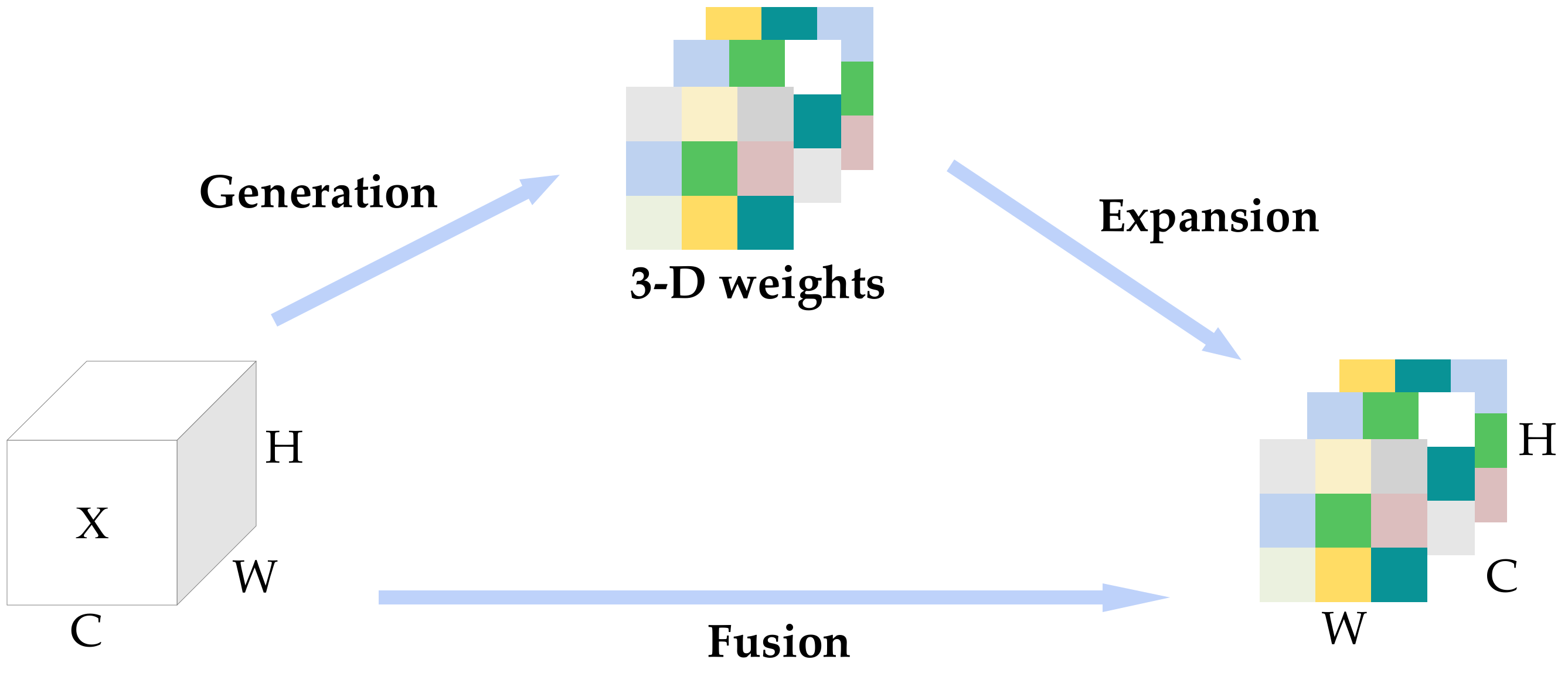
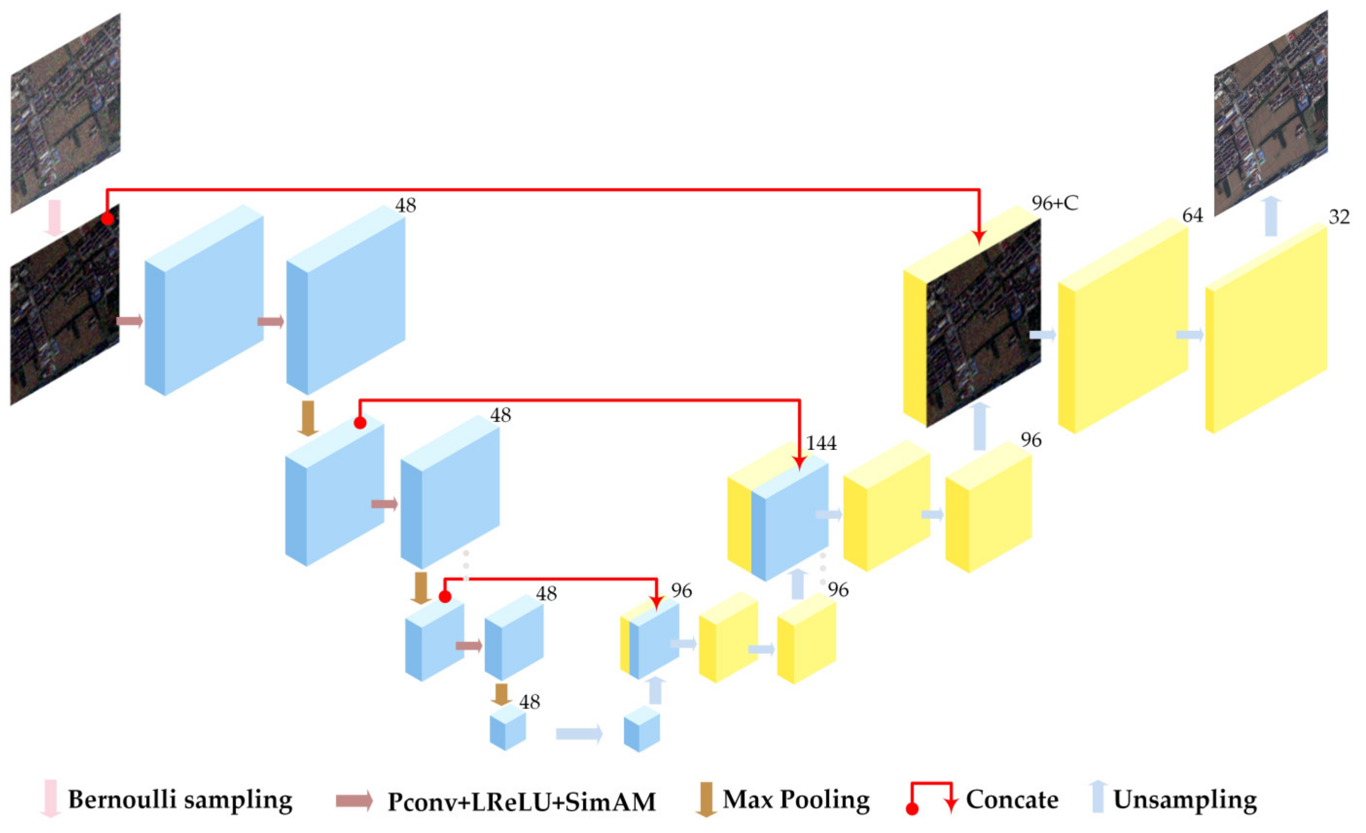
- We propose a self-supervised image-denoising method designed explicitly for RS images. This network leverages information from both the spatial and channel dimensions of RS images and is trained using only one image, without additional parameters. It effectively handles mixed-noise scenarios, reconstructing noise-reduced RS images while preserving detailed texture information. The method strikes a favorable balance between noise reduction and detail preservation, resulting in satisfactory denoising performance. This approach is particularly well suited for subsequent CD tasks;
- (3)
- The CD component of the proposed framework comprises two techniques, FCM_SICM and EMD, that synergistically exhibit good noise resilience. Experimental results demonstrate that the FCM_SICM-EMD method is robust and effective for performing CD tasks under noisy conditions.
2. Materials and Methods
2.1. Overview
2.2. SSDNet
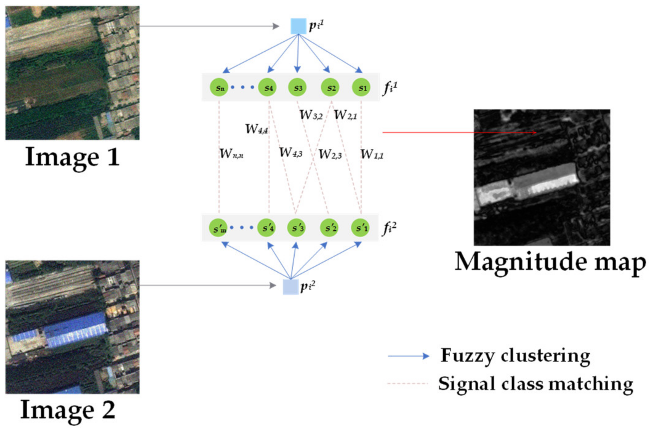
2.3. FCM_SICM-EMD
2.3.1. FCM_SICM
2.3.2. EMD
3. Dataset and Experimental Setup
3.1. Dataset Descriptions
- (1)
- For the Shangtang dataset, this dataset is obtained from the SenseEarth platform dataset used in the AI Vision of the World 2020 Artificial Intelligence Remote Sensing Interpretation Competition hosted by SenseTime Technology [45]. Its image size is 512 × 512 pixels, with a spatial resolution of 3 m. The selected study area comprises images of rural areas containing four land-cover types, buildings, farmland, woodland, and wasteland, among which the major changes involve the construction of buildings;
- (2)
- For the DSIFN-CD dataset, this dataset is manually collected from Google Earth. It consists of six large bitemporal high-resolution images covering six cities in China (Beijing, Chengdu, Shenzhen, Chongqing, Wuhan, and Xi’an) [46]. Five large image pairs are cropped into sub-image pairs of size 512 × 512 with a spatial resolution of 2 m/pixel, followed by data augmentation. The selected study area includes five land-cover types, namely roads, farmland, wasteland, buildings, and vegetation, where the primary changes happen in wasteland and vegetation areas;
- (3)
- For the LZ dataset, this dataset comprises two Landsat8 images from the Lanzhou New Area in China, captured in 2016 and 2017, respectively [47]. These images display seven bands with a spatial resolution of 30 m and a size of 650 × 650 pixels. The scenes in these images include forests, farmland, wastelands, mountains, and buildings;
- (4)
- For the CDD dataset, the CDD dataset consists of real RS images with seasonal variations (obtained from Google Earth), including four high-resolution images captured in four seasons [48]. A pair of images with a size of 1900 × 1000 pixels form the study area and are manually cropped to 992 × 992 pixels with a spatial resolution of 0.3–1 m/pixel, containing water bodies, buildings, forests, and grasslands, among which the dominant changes happen in areas of buildings and forests;
- (5)
- For the GZ dataset, this dataset covers the suburban area of Guangzhou, China, collected between 2006 and 2019 [49]. A total of 19 bitemporal high-resolution images with red, green, and blue bands, a spatial resolution of 0.55 m, and a size of 1006 × 1168 are collected using the BIGEMAP (30.0.31.6) software and Google Earth service. These images are manually cropped into sub-image pairs of size 1024 × 1024, in which the major changes are caused by urban development.
3.2. Competing Methods
3.3. Experimental Design and Evaluation Metrics
4. Experimental Results
4.1. Noise-Resistance Analysis
4.2. Noise Sensitivity Analysis

4.3. Ablation Analysis
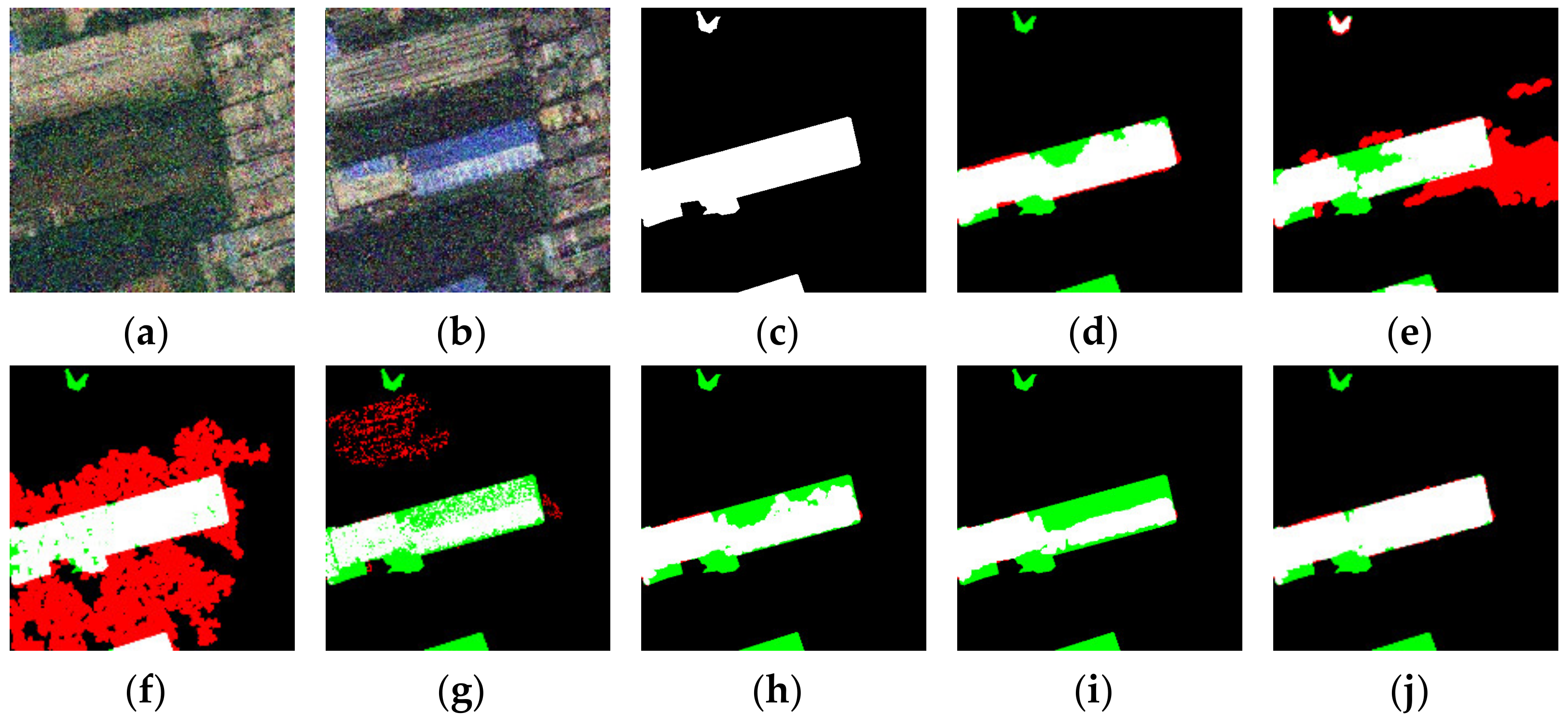
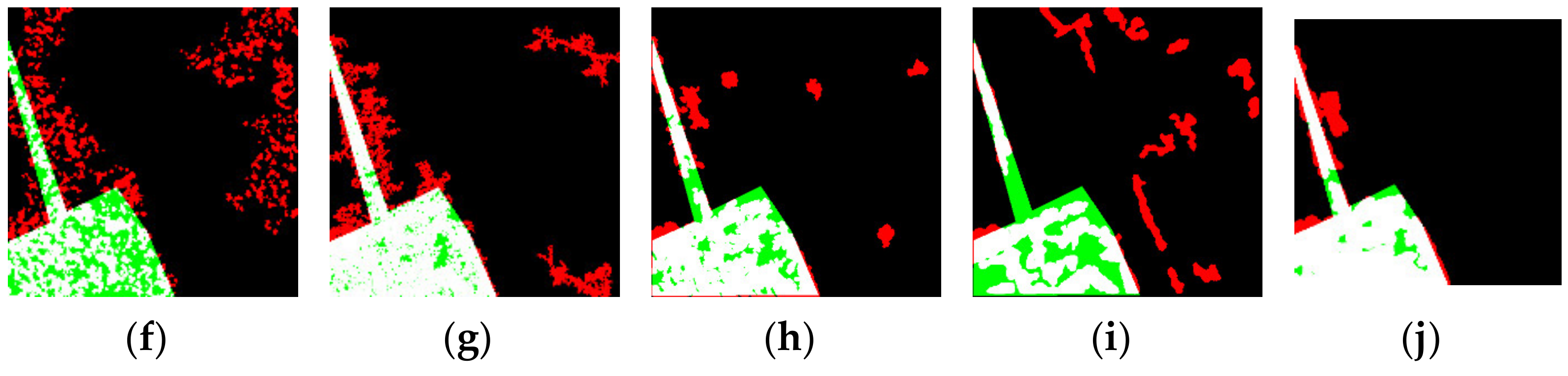
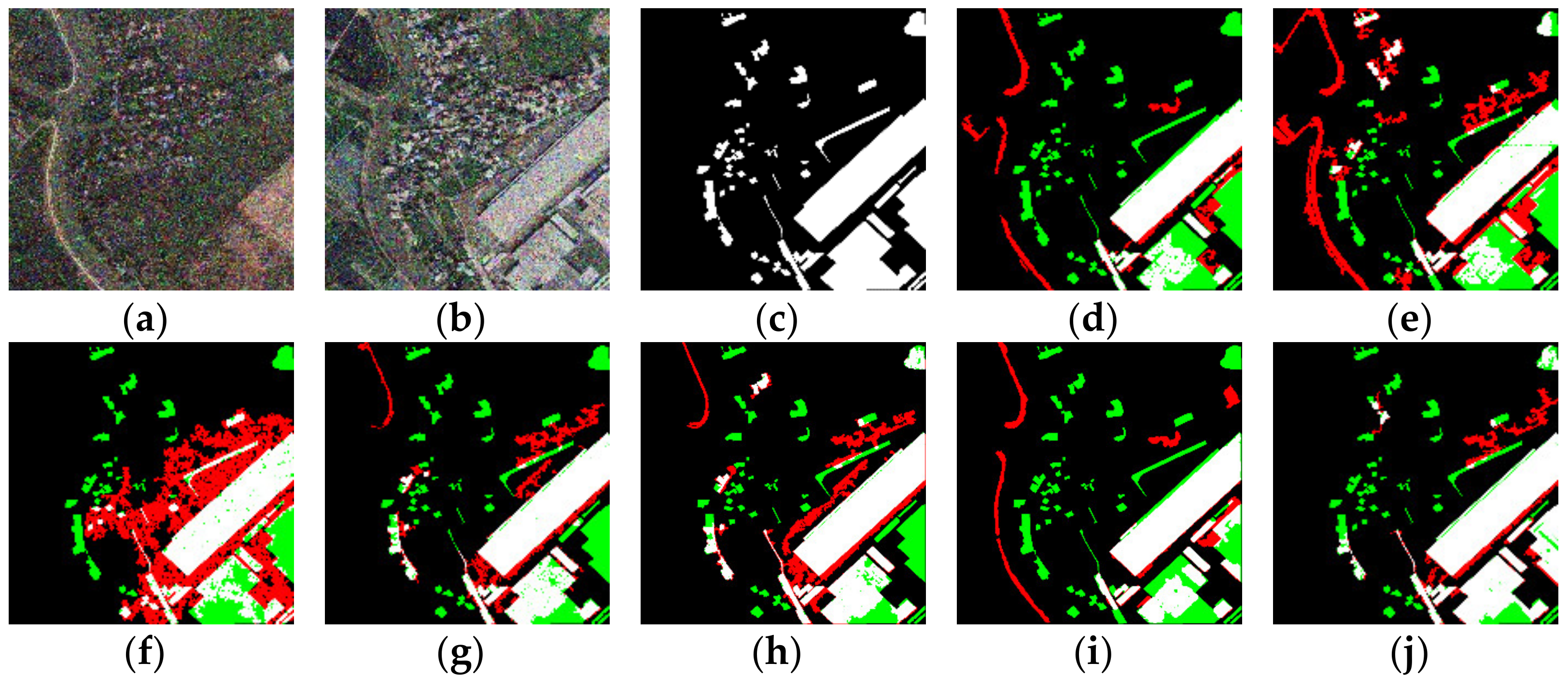
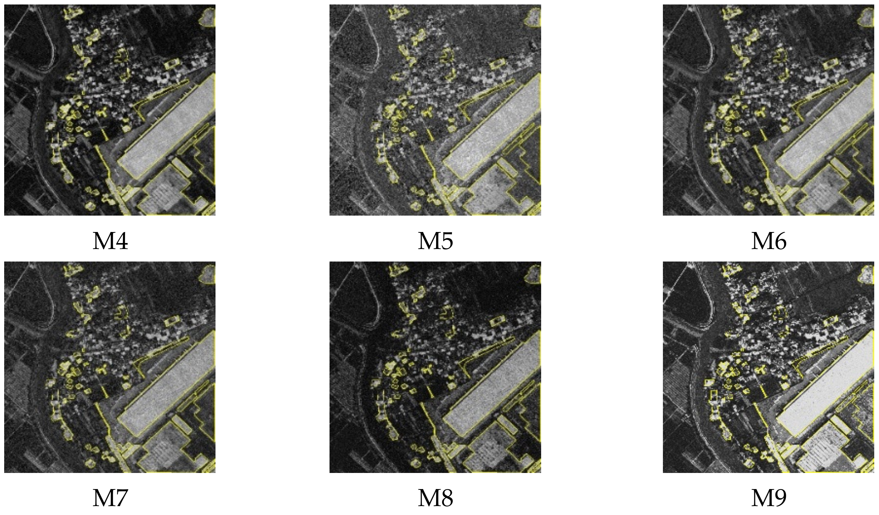
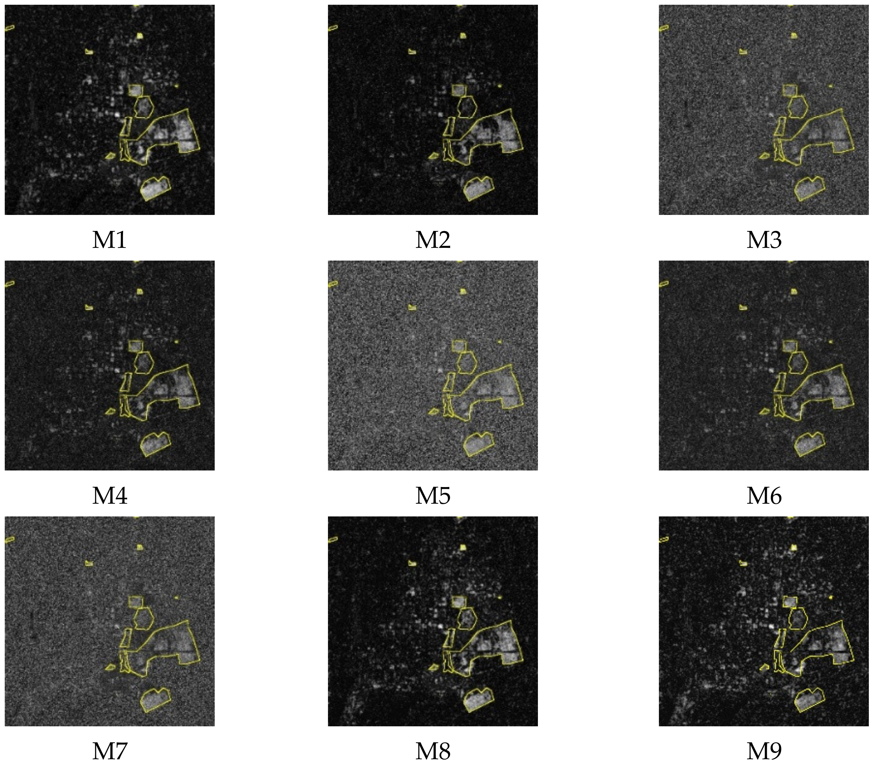
4.4. Analysis of Change-Magnitude Maps
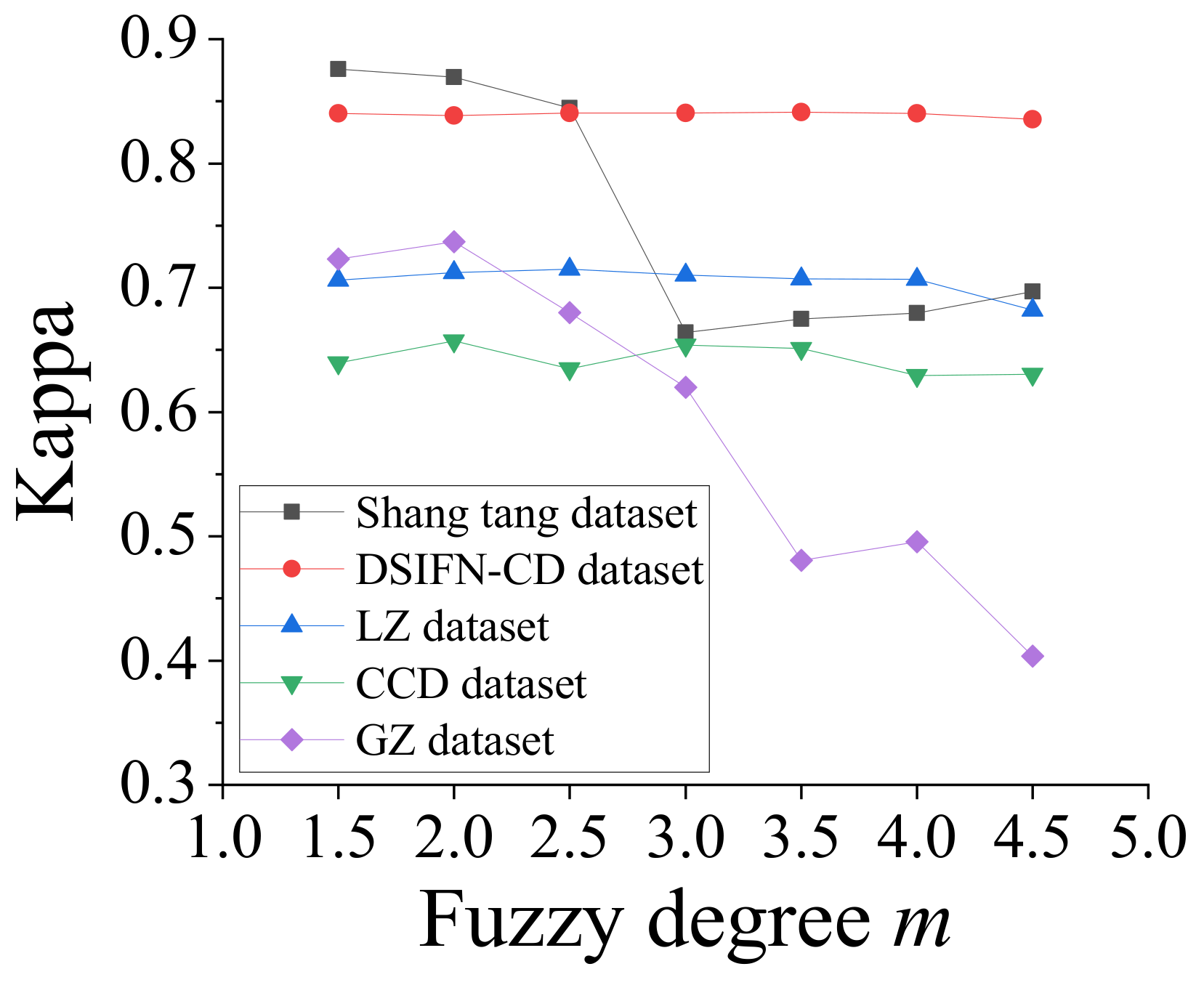
4.5. Sensitivity Analysis of the Fuzziness Levels
4.6. Computational Time
5. Conclusions
Author Contributions
Funding
Data Availability Statement
Acknowledgments
Conflicts of Interest
References
- Caiza-Morales, L.; Gómez, C.; Torres, R.; Nicolau, A.P.; Olano, J.M. Manglee: A tool for mapping and monitoring Mangrove ecosystem on google earth engine—A case study in ecuador. J. Geovisualization Spat. Anal. 2024, 8, 17. [Google Scholar] [CrossRef]
- Zhi, Z.; Liu, J.; Liu, J.; Li, A. Geospatial structure and evolution analysis of national terrestrial adjacency network based on complex network. J. Geovisualization Spat. Anal. 2024, 8, 12. [Google Scholar] [CrossRef]
- Yang, J.; Huang, X. 30 m Annual land cover and its dynamics in China from 1990 to 2019. Earth Syst. Sci. Data Discuss. 2021, 13, 3907–3925. [Google Scholar] [CrossRef]
- Qin, X.; He, S.; Yang, X.; Dehghan, M.; Qin, Q.; Martin, J. Accurate outline extraction of individual building from Very High-Resolution optical images. IEEE Geosci. Remote Sens. Lett. 2018, 15, 1775–1779. [Google Scholar] [CrossRef]
- Li, X.; Ling, F.; Giles, M.F.; Du, Y. A superresolution Land-Cover change detection method using remotely sensed images with different spatial resolutions. IEEE Trans. Geosci. Remote Sens. 2016, 54, 3822–3841. [Google Scholar] [CrossRef]
- Qu, Y.; Li, J.; Huang, X.; Wen, D. TD-SSCD: A novel network by fusing temporal and differential information for self-supervised remote sensing image change detection. IEEE Trans. Geosci. Remote Sens. 2023, 61, 5407015. [Google Scholar] [CrossRef]
- Zhao, Y.; Wang, G.; Yang, J.; Li, T.; Li, Z. Au3-gan: A method for extracting roads from historical maps based on an attention generative adversarial network. J. Geovisualization Spat. Anal. 2024, 8, 26. [Google Scholar] [CrossRef]
- Lu, D.; Mausel, P.; Brondizio, E.; Moran, E. Change detection techniques. Int. J. Remote Sens. 2004, 25, 2365–2401. [Google Scholar] [CrossRef]
- Ma, J.; Gong, M.; Zhou, Z. Wavelet fusion on ratio images for change detection in SAR images. IEEE Geosci. Remote Sens. Lett. 2012, 9, 1122–1126. [Google Scholar] [CrossRef]
- Bovolo, F.; Bruzzone, L. A theoretical framework for unsupervised change detection based on change vector analysis in the polar domain. IEEE Trans. Geosci. Remote Sens. 2007, 45, 218–236. [Google Scholar] [CrossRef]
- Deng, J.; Wang, K.; Deng, Y.; Qi, G. PCA-Based land use change detection and analysis using multitemporal and multisensor satellite data. Int. J. Remote Sens. 2008, 29, 4823–4838. [Google Scholar] [CrossRef]
- Nielsen, A.A.; Conradsen, K.; Simpson, J.J. Multivariate alteration detection (MAD) and MAF postprocessing in multispectral, bitemporal image data: New approaches to change detection studies. Remote Sens. Environ. 1998, 64, 1–19. [Google Scholar] [CrossRef]
- Marpu, P.R.; Gamba, P.; Canty, M.J. Improving change detection results of IR-MAD by eliminating strong changes. IEEE Geosci. Remote Sens. Lett. 2011, 8, 799–803. [Google Scholar] [CrossRef]
- Celik, T. Unsupervised change detection in satellite images using principal component analysis and K-Means clustering. IEEE Geosci. Remote Sens. Lett. 2009, 6, 772–776. [Google Scholar] [CrossRef]
- Chen, P.; Li, C.; Zhang, B.; Chen, Z.; Yang, X.; Lu, K.; Zhuang, L. A region-based feature fusion network for VHR image change detection. Remote Sens. 2022, 14, 5577. [Google Scholar] [CrossRef]
- Wang, J.; Zhao, T.; Jiang, X.; Lan, K. A hierarchical heterogeneous graph for unsupervised SAR image change detection. IEEE Geosci. Remote Sens. Lett. 2022, 19, 4516605. [Google Scholar] [CrossRef]
- Zhao, H.; Liu, S.; Du, Q.; Bruzzone, L.; Zheng, Y.; Du, K.; Tong, X.; Xie, H.; Ma, X. GCFnet: Global collaborative fusion network for multispectral and panchromatic image classification. IEEE Trans. Geosci. Remote Sens. 2022, 60, 5632814. [Google Scholar] [CrossRef]
- Zhang, H.; Yao, J.; Ni, L.; Gao, L.; Huang, M. Multimodal attention-aware convolutional neural networks for classification of hyperspectral and LiDAR data. IEEE J. Sel. Top. Appl. Earth Obs. Remote Sens. 2023, 16, 3635–3644. [Google Scholar] [CrossRef]
- Tang, X.; Zhang, H.; Mou, L.; Liu, F.; Zhang, X.; Zhu, X.; Jiao, L. An unsupervised remote sensing change detection method based on multiscale graph convolutional network and metric learning. IEEE Trans. Geosci. Remote Sens. 2022, 60, 5632814. [Google Scholar] [CrossRef]
- Wu, C.; Chen, H.; Du, B.; Zhang, L. Unsupervised change detection in multitemporal VHR images based on deep kernel PCA convolutional mapping network. IEEE Trans. Cyber. 2022, 52, 12084–12098. [Google Scholar] [CrossRef]
- Saha, S.; Bovolo, F.; Bruzzone, L. Unsupervised deep change vector analysis for multiple-change detection in VHR images. IEEE Trans. Geosci. Remote Sens. 2019, 57, 3677–3693. [Google Scholar] [CrossRef]
- Ke, Q.; Zhang, P. Hybrid-transCD: A hybrid transformer remote sensing image change detection network via token aggregation. ISPRS Int. J. Geo-Inf. 2022, 11, 263. [Google Scholar] [CrossRef]
- Li, Q.; Zhong, R.; Du, X.; Du, Y. TransUNetCD: A hybrid transformer network for change detection in optical remote-sensing images. IEEE Trans. Geosci. Remote Sens. 2022, 60, 5622519. [Google Scholar] [CrossRef]
- Lin, Y.; Liu, S.; Zheng, Y.; Tong, X.; Xie, H.; Zhu, H.; Du, K.; Zhao, H.; Zhang, J. An unsupervised transformer-based multivariate alteration detection approach for change detection in VHR remote sensing images. IEEE J. Sel. Top. Appl. Earth Obs. Remote Sens. 2024, 17, 3251–3261. [Google Scholar] [CrossRef]
- Liu, M.; Jiang, W.; Liu, W.; Tao, D.; Liu, B. Dynamic adaptive attention-guided self-supervised single remote-sensing image denoising. IEEE Trans. Geosci. Remote Sens. 2023, 61, 4704511. [Google Scholar] [CrossRef]
- Gu, S.; Li, Y.; Gool, L.V.; Timofte, R. Self-guided network for fast image denoising. In Proceedings of the IEEE/CVF International Conference on Computer Vision, Seoul, Republic of Korea, 27 October–2 November 2019; pp. 2511–2520. [Google Scholar]
- Zhang, K.; Zuo, W.; Chen, Y.; Meng, D.; Zhang, L. Beyond a Gaussian Denoiser: Residual learning of deep CNN for image denoising. IEEE Trans. Image Process. 2017, 26, 3142–3155. [Google Scholar] [CrossRef]
- Zhao, Y.; Jiang, Z.; Men, A.; Ju, G. Pyramid real image denoising network. In Proceedings of the 2019 IEEE Visual Communications and Image Processing (VCIP), Sydney, NSW, Australia, 1–4 December 2019; pp. 1–4. [Google Scholar]
- Jia, X.; Peng, Y.; Li, J.; Ge, B.; Xin, Y.; Liu, S. Dual-complementary convolution network for remote-sensing image denoising. IEEE Geosci. Remote Sens. Lett. 2022, 19, 8018405. [Google Scholar] [CrossRef]
- Tai, Y.; Yang, J.; Liu, X.; Xu, C. Memnet: A persistent memory network for image restoration. In Proceedings of the IEEE International Conference on Computer Vision, Venice, Italy, 22–29 October 2017; pp. 4539–4547. [Google Scholar]
- Wang, Y.; Song, X.; Chen, K. Channel and space attention neural network for image denoising. IEEE Signal Process Lett. 2021, 28, 424–428. [Google Scholar] [CrossRef]
- Dabov, K.; Foi, A.; Katkovnik, V.; Egiazarian, K. Color image denoising via sparse 3D collaborative filtering with grouping constraint in luminance-chrominance space. In Proceedings of the 2007 IEEE International Conference on Image Processing, San Antonio, TX, USA, 16 September–19 October 2007; pp. 313–316. [Google Scholar]
- Li, Y.; Li, X.; Song, J.; Wang, Z.; He, Y.; Yang, S. Remote-sensing-based change detection using change vector analysis in posterior probability space: A context-sensitive bayesian network approach. IEEE J. Sel. Top. Appl. Earth Obs. Remote Sens. 2023, 16, 3198–3217. [Google Scholar] [CrossRef]
- Wang, Q.; Wang, X.; Fang, C.; Yang, W. Robust fuzzy C-means clustering algorithm with adaptive spatial & intensity constraint and membership linking for noise image segmentation. Appl. Soft Comput. 2020, 92, 106318. [Google Scholar]
- Rubner, Y.; Tomasi, C.; Guibas, L.J. A metric for distributions with applications to image databases. In Proceedings of the Sixth International Conference on Computer Vision (IEEE Cat. No.98CH36271), Bombay, India, 7 January 1998; pp. 59–66. [Google Scholar]
- Quan, Y.; Chen, M.; Pang, T.; Ji, H. Self2self with dropout: Learning self-supervised denoising from single image. In Proceedings of the IEEE/CVF Conference on Computer Vision and Pattern Recognition, Seattle, WA, USA, 13–19 June 2020; pp. 1890–1898. [Google Scholar]
- Yang, L.; Zhang, R.; Li, L.; Xie, X. SimAM: A simple, parameter-free attention module for convolutional neural networks. In Proceedings of the IEEE International Conference on Machine Learning, Online, 18–24 July 2021; pp. 11863–11874. [Google Scholar]
- Lehtinen, J.; Munkberg, J.; Hasselgren, J.; Laine, S.; Karras, T.; Aittala, M.; Aila, T. Noise2noise: Learning image restoration without clean data. arXiv 2018, arXiv:1803.04189. [Google Scholar]
- Huang, T.; Li, S.; Jia, X.; Lu, H.; Liu, J. Neighbor2neighbor: Self-supervised denoising from single noisy images. In Proceedings of the IEEE/CVF Conference on Computer Vision and Pattern Recognition, Nashville, TN, USA, 20–25 June 2021; pp. 14781–14790. [Google Scholar]
- Krull, A.; Buchholz, T.O.; Jug, F. Noise2void-learning denoising from single noisy images. In Proceedings of the IEEE/CVF Conference on Computer Vision and Pattern Recognition, Long Beach, CA, USA, 15–20 June 2019; pp. 2129–2137. [Google Scholar]
- Chen, Y.; Bruzzone, L. Self-supervised change detection in multiview remote sensing images. IEEE Trans. Geosci. Remote Sens. 2022, 60, 1–12. [Google Scholar] [CrossRef]
- Wang, W.; Tan, X.; Zhang, P.; Wang, X. A CBAM based multiscale transformer fusion approach for remote sensing image change detection. IEEE J. Sel. Top. Appl. Earth Obs. Remote Sens. 2022, 15, 6817–6825. [Google Scholar] [CrossRef]
- Ahmed, M.N.; Yamany, S.M.; Mohamed, N.; Farag, A.A.; Moriarty, T. A modified fuzzy c-means algorithm for bias field estimation and segmentation of MRI data. IEEE Trans. Med. Imaging 2002, 3, 193–199. [Google Scholar] [CrossRef] [PubMed]
- Chaudhury, K.N.; Dabhade, S.D. Fast and provably accurate bilateral filtering. IEEE Trans. Image Process. 2016, 25, 2519–2528. [Google Scholar] [CrossRef] [PubMed]
- SenseEarth. Available online: https://rs.sensetime.com/ (accessed on 20 March 2024).
- Zhang, C.; Yue, P.; Tapete, D.; Jiang, L.; Shangguan, B.; Huang, L.; Liu, G. A deeply supervised image fusion network for change detection in high resolution bi-temporal remote sensing images. ISPRS J. Photogram. Remote Sens. 2020, 166, 183–200. [Google Scholar] [CrossRef]
- Geospatial Data Cloud. Available online: https://www.gscloud.cn/sources/ (accessed on 5 June 2022).
- Lebedev, M.A.; Vizilter, Y.V.; Vygolov, O.V.; Knyaz, V.A.; Rubis, A.Y. Change detection in remote sensing images using conditional adversarial networks. Int. Arch. Photogram. Remote Sens. Spat. Inf. Sci. 2018, 42, 565–571. [Google Scholar] [CrossRef]
- Fan, R.; Xie, J.; Yang, J.; Hong, Z.; Xu, Y.; Hou, H. Multiscale change detection domain adaptation model based on illumination–reflection decoupling. Remote Sens. 2024, 16, 799. [Google Scholar] [CrossRef]
- Lv, Z.; Wang, F.; Liu, T.; Kong, X.; Benediktsson, J.A. Novel automatic approach for land cover change detection by using VHR remote sensing images. IEEE Geosci. Remote Sens. Lett. 2021, 19, 8016805. [Google Scholar] [CrossRef]
- Sun, Y.; Lei, L.; Li, X.; Tan, X.; Kuang, G. Structure consistency-based graph for unsupervised change detection with homogeneous and heterogeneous remote sensing images. IEEE Trans. Geosci. Remote Sens. 2022, 60, 4700221. [Google Scholar] [CrossRef]
- Lv, Z.Y.; Liu, T.; Zhang, P.; Benediktsson, J.A.; Lei, T.; Zhang, X. Novel adaptive histogram trend similarity approach for land cover change detection by using bitemporal very-high-resolution remote sensing images. IEEE Trans. Geosci. Remote Sens. 2019, 57, 9554–9574. [Google Scholar] [CrossRef]
- Krinidis, S.; Chatzis, V. A robust fuzzy local information C-means clustering algorithm. IEEE Trans. Image Process. 2010, 19, 1328–1337. [Google Scholar] [CrossRef] [PubMed]
- Chen, S.; Zhang, D. Robust image segmentation using FCM with spatial constraints based on new kernel-induced distance measure. IEEE Trans. Syst. Man Cyber. Part B 2004, 34, 1907–1916. [Google Scholar] [CrossRef] [PubMed]


| Dataset | Method | Evaluation Metrics | |||||
|---|---|---|---|---|---|---|---|
| FA | MA | OA | Kappa | Recall | F1 | ||
| Shangtang | GMCD [19] | 0.0633 | 0.2307 | 0.9574 | 0.8204 | 0.7546 | 0.8374 |
| KPCAMNet [20] | 0.4310 | 0.2204 | 0.8777 | 0.5856 | 0.7635 | 0.6279 | |
| DCVA [21] | 0.6848 | 0.0661 | 0.6839 | 0.3173 | 0.9313 | 0.4782 | |
| PCAKMeans [22] | 0.2042 | 0.4128 | 0.9150 | 0.6281 | 0.5752 | 0.6598 | |
| ASEA [50] | 0.0144 | 0.3271 | 0.9491 | 0.7717 | 0.6591 | 0.7900 | |
| INLPG [51] | 0.0084 | 0.4670 | 0.9288 | 0.6571 | 0.5194 | 0.6815 | |
| Ours | 0.0303 | 0.1637 | 0.9714 | 0.8816 | 0.8211 | 0.8902 | |
| DSIFN-CD | GMCD [19] | 0.3762 | 0.1495 | 0.8831 | 0.6481 | 0.8357 | 0.7365 |
| KPCAMNet [20] | 0.5956 | 0.5465 | 0.7857 | 0.2963 | 0.5975 | 0.5962 | |
| DCVA [21] | 0.5110 | 0.4443 | 0.8192 | 0.4094 | 0.5614 | 0.5414 | |
| PCAKMeans [22] | 0.3535 | 0.1013 | 0.8954 | 0.6880 | 0.8974 | 0.7701 | |
| ASEA [50] | 0.1875 | 0.1981 | 0.9323 | 0.7661 | 0.7967 | 0.8114 | |
| INLPG [51] | 0.3635 | 0.4108 | 0.8681 | 0.5326 | 0.5842 | 0.6479 | |
| Ours | 0.1750 | 0.0928 | 0.9497 | 0.8333 | 0.9040 | 0.8466 | |
| Dataset | Method | Evaluation Metrics | |||||
|---|---|---|---|---|---|---|---|
| FA | MA | OA | Kappa | Recall | F1 | ||
| LZ | GMCD [19] | 0.7661 | 0.0599 | 0.7750 | 0.2935 | 0.9506 | 0.3918 |
| KPCAMNet [20] | 0.2671 | 0.2603 | 0.9620 | 0.7159 | 0.7764 | 0.7480 | |
| DCVA [21] | 0.9069 | 0.0756 | 0.3495 | 0.0448 | 0.9275 | 0.1744 | |
| PCAKMeans [22] | 0.8364 | 0.0130 | 0.6373 | 0.1798 | 0.9936 | 0.3028 | |
| ASEA [50] | 0.0529 | 0.5926 | 0.9558 | 0.5502 | 0.4028 | 0.5653 | |
| INLPG [51] | 0.0699 | 0.5903 | 0.9554 | 0.5490 | 0.4110 | 0.5701 | |
| Ours | 0.1845 | 0.2267 | 0.9712 | 0.7784 | 0.8079 | 0.8159 | |
| Dataset | Method | Evaluation Metrics | |||||
|---|---|---|---|---|---|---|---|
| FA | MA | OA | Kappa | Recall | F1 | ||
| CDD | GMCD [19] | 0.2550 | 0.3704 | 0.9439 | 0.6519 | 0.6203 | 0.6924 |
| KPCAMNet [20] | 0.3643 | 0.3320 | 0.9316 | 0.6135 | 0.6529 | 0.6642 | |
| DCVA [21] | 0.8716 | 0.7507 | 0.7661 | 0.0494 | 0.2036 | 0.1624 | |
| PCAKMeans [22] | 0.6292 | 0.2314 | 0.8530 | 0.4261 | 0.7932 | 0.5109 | |
| ASEA [50] | 0.2476 | 0.4179 | 0.9416 | 0.6250 | 0.5763 | 0.6680 | |
| INLPG [51] | 0.2094 | 0.5504 | 0.9358 | 0.5413 | 0.4571 | 0.5961 | |
| Ours | 0.2905 | 0.3283 | 0.9422 | 0.6582 | 0.6653 | 0.7034 | |
| GZ | GMCD [19] | 0.2783 | 0.4764 | 0.8659 | 0.5285 | 0.5496 | 0.6444 |
| KPCAMNet [20] | 0.4610 | 0.4058 | 0.8194 | 0.4516 | 0.5975 | 0.5962 | |
| DCVA [21] | 0.5768 | 0.3769 | 0.7577 | 0.3514 | 0.6400 | 0.5326 | |
| PCAKMeans [22] | 0.2626 | 0.3506 | 0.8850 | 0.6204 | 0.6630 | 0.7106 | |
| ASEA [50] | 0.2902 | 0.3111 | 0.8828 | 0.6263 | 0.7039 | 0.7231 | |
| INLPG [51] | 0.2186 | 0.4202 | 0.8848 | 0.5979 | 0.6275 | 0.7147 | |
| Ours | 0.1774 | 0.2409 | 0.9200 | 0.7403 | 0.8199 | 0.8243 | |
| Dataset | Method | Mixed-Noise Level | ||||||
|---|---|---|---|---|---|---|---|---|
| 0.00 | 0.01 | 0.02 | 0.03 | 0.04 | 0.05 | 0.06 | ||
| Shangtang | GMCD [19] | 0.6678 | 0.5546 | 0.6420 | 0.7324 | 0.7538 | 0.7774 | 0.7776 |
| KPCAMNet [20] | 0.5706 | 0.5784 | 0.5913 | 0.6210 | 0.5829 | 0.5769 | 0.5415 | |
| DCVA [21] | 0.1851 | 0.3195 | 0.2801 | 0.2727 | 0.2598 | 0.2473 | 0.1798 | |
| PCAKMeans [22] | 0.6677 | 0.6858 | 0.7955 | 0.8556 | 0.7308 | 0.4398 | 0.2600 | |
| ASEA [50] | 0.6507 | 0.6990 | 0.7508 | 0.7316 | 0.7701 | 0.7717 | 0.7544 | |
| INLPG [51] | 0.5107 | 0.5154 | 0.6330 | 0.6376 | 0.6552 | 0.6571 | 0.6552 | |
| Ours | 0.8626 | 0.8624 | 0.8641 | 0.8573 | 0.8789 | 0.8795 | 0.8606 | |
| DSIFN-CD | GMCD [19] | 0.6918 | 0.5258 | 0.4653 | 0.4949 | 0.5892 | 0.5957 | 0.5941 |
| KPCAMNet [20] | 0.1384 | 0.1924 | 0.3010 | 0.3408 | 0.3596 | 0.3228 | 0.3268 | |
| DCVA [21] | 0.4887 | 0.3119 | 0.3011 | 0.2941 | 0.2974 | 0.2862 | 0.2762 | |
| PCAKMeans [22] | 0.8561 | 0.7324 | 0.7837 | 0.7561 | 0.7494 | 0.6021 | 0.4905 | |
| ASEA [50] | 0.7311 | 0.7345 | 0.7411 | 0.7699 | 0.7648 | 0.7661 | 0.7602 | |
| INLPG [51] | 0.1260 | 0.3168 | 0.3799 | 0.4625 | 0.5454 | 0.5326 | 0.6376 | |
| Ours | 0.8398 | 0.8244 | 0.8447 | 0.8393 | 0.8356 | 0.8333 | 0.8085 | |
| LZ | GMCD [19] | 0.6684 | 0.6674 | 0.6419 | 0.3911 | 0.2572 | 0.2038 | 0.1525 |
| KPCAMNet [20] | 0.6888 | 0.6540 | 0.6401 | 0.6512 | 0.6922 | 0.6902 | 0.6886 | |
| DCVA [21] | 0.3192 | 0.0815 | 0.0556 | 0.0372 | 0.0388 | 0.0448 | 0.0406 | |
| PCAKMeans [22] | 0.7862 | 0.7033 | 0.3171 | 0.2038 | 0.1726 | 0.1645 | 0.1383 | |
| ASEA [50] | 0.7387 | 0.6581 | 0.6441 | 0.6593 | 0.5657 | 0.5502 | 0.5099 | |
| INLPG [51] | 0.4399 | 0.5621 | 0.6427 | 0.6473 | 0.5634 | 0.5490 | 0.6479 | |
| Ours | 0.7873 | 0.7917 | 0.7904 | 0.6856 | 0.7849 | 0.7796 | 0.7806 | |
| CDD | GMCD [19] | 0.5946 | 0.6166 | 0.6339 | 0.6476 | 0.6524 | 0.6534 | 0.6249 |
| KPCAMNet [20] | 0.5726 | 0.5966 | 0.6129 | 0.6144 | 0.6052 | 0.6044 | 0.6072 | |
| DCVA [21] | 0.0173 | 0.0318 | 0.0461 | 0.0412 | 0.0251 | 0.0252 | 0.0258 | |
| PCAKMeans [22] | 0.6029 | 0.6326 | 0.5821 | 0.4475 | 0.2793 | 0.2568 | 0.1395 | |
| ASEA [50] | 0.5597 | 0.5901 | 0.6021 | 0.6139 | 0.6188 | 0.6250 | 0.6007 | |
| INLPG [51] | 0.4930 | 0.4948 | 0.5057 | 0.5201 | 0.5509 | 0.5413 | 0.5334 | |
| Ours | 0.6234 | 0.6354 | 0.6372 | 0.6218 | 0.6476 | 0.6431 | 0.6392 | |
| GZ | GMCD [19] | 0.5351 | 0.5392 | 0.5164 | 0.5506 | 0.5392 | 0.5285 | 0.5448 |
| KPCAMNet [20] | 0.4259 | 0.4174 | 0.4389 | 0.4493 | 0.4633 | 0.4516 | 0.4694 | |
| DCVA [21] | 0.2324 | 0.3471 | 0.3185 | 0.2897 | 0.2584 | 0.3514 | 0.2101 | |
| PCAKMeans [22] | 0.6194 | 0.6385 | 0.6367 | 0.6331 | 0.6255 | 0.6204 | 0.6199 | |
| ASEA [50] | 0.6122 | 0.6161 | 0.6139 | 0.6182 | 0.6292 | 0.6263 | 0.6272 | |
| INLPG [51] | 0.5294 | 0.5899 | 0.6122 | 0.6020 | 0.5961 | 0.5979 | 0.6090 | |
| Ours | 0.7551 | 0.7485 | 0.7451 | 0.7468 | 0.7439 | 0.7403 | 0.7393 | |
| Method | FA | MA | OA | Kappa | Rec | F1 |
|---|---|---|---|---|---|---|
| M1 | 0.1774 | 0.2409 | 0.9200 | 0.7403 | 0.8199 | 0.8243 |
| M2 | 0.2367 | 0.2342 | 0.9067 | 0.7064 | 0.7947 | 0.7884 |
| M3 | 0.3648 | 0.2763 | 0.8632 | 0.5902 | 0.7356 | 0.7084 |
| M4 | 0.3484 | 0.2678 | 0.8696 | 0.6073 | 0.7352 | 0.7153 |
| M5 | 0.5470 | 0.1847 | 0.7689 | 0.4401 | 0.8212 | 0.6397 |
| M6 | 0.3399 | 0.2739 | 0.8719 | 0.6109 | 0.7290 | 0.7185 |
| M7 | 0.2510 | 0.3487 | 0.8879 | 0.6284 | 0.6762 | 0.7232 |
| M8 | 0.2327 | 0.3281 | 0.8948 | 0.6522 | 0.6998 | 0.7423 |
| M9 | 0.1748 | 0.3219 | 0.9079 | 0.6889 | 0.7343 | 0.7801 |
| Dataset | Fuzzy Degree | ||||||
|---|---|---|---|---|---|---|---|
| 1.5 | 2.0 | 2.5 | 3.0 | 3.5 | 4.0 | 4.5 | |
| Shangtang [45] | 0.8758 | 0.8694 | 0.8446 | 0.6638 | 0.6749 | 0.6797 | 0.6968 |
| DSIFN-CD [46] | 0.8402 | 0.8383 | 0.8405 | 0.8404 | 0.8412 | 0.8401 | 0.8353 |
| LZ [47] | 0.7059 | 0.7123 | 0.7150 | 0.7102 | 0.7071 | 0.7067 | 0.6820 |
| CDD [48] | 0.6394 | 0.6573 | 0.6349 | 0.6538 | 0.6510 | 0.6293 | 0.6303 |
| GZ [49] | 0.7230 | 0.7371 | 0.6801 | 0.6200 | 0.4806 | 0.4955 | 0.4034 |
Disclaimer/Publisher’s Note: The statements, opinions and data contained in all publications are solely those of the individual author(s) and contributor(s) and not of MDPI and/or the editor(s). MDPI and/or the editor(s) disclaim responsibility for any injury to people or property resulting from any ideas, methods, instructions or products referred to in the content. |
© 2024 by the authors. Licensee MDPI, Basel, Switzerland. This article is an open access article distributed under the terms and conditions of the Creative Commons Attribution (CC BY) license (https://creativecommons.org/licenses/by/4.0/).
Share and Cite
Xie, J.; Li, Y.; Yang, S.; Li, X. Unsupervised Noise-Resistant Remote-Sensing Image Change Detection: A Self-Supervised Denoising Network-, FCM_SICM-, and EMD Metric-Based Approach. Remote Sens. 2024, 16, 3209. https://doi.org/10.3390/rs16173209
Xie J, Li Y, Yang S, Li X. Unsupervised Noise-Resistant Remote-Sensing Image Change Detection: A Self-Supervised Denoising Network-, FCM_SICM-, and EMD Metric-Based Approach. Remote Sensing. 2024; 16(17):3209. https://doi.org/10.3390/rs16173209
Chicago/Turabian StyleXie, Jiangling, Yikun Li, Shuwen Yang, and Xiaojun Li. 2024. "Unsupervised Noise-Resistant Remote-Sensing Image Change Detection: A Self-Supervised Denoising Network-, FCM_SICM-, and EMD Metric-Based Approach" Remote Sensing 16, no. 17: 3209. https://doi.org/10.3390/rs16173209
APA StyleXie, J., Li, Y., Yang, S., & Li, X. (2024). Unsupervised Noise-Resistant Remote-Sensing Image Change Detection: A Self-Supervised Denoising Network-, FCM_SICM-, and EMD Metric-Based Approach. Remote Sensing, 16(17), 3209. https://doi.org/10.3390/rs16173209