Improved Winter Wheat Yield Estimation by Combining Remote Sensing Data, Machine Learning, and Phenological Metrics

Abstract

Accurate yield prediction is essential for global food security and effective agricultural management. Traditional empirical statistical models and crop models face significant limitations, including high computational demands and dependency on high-resolution soil and daily weather data, that restrict their scalability across different temporal and spatial scales. Moreover, the lack of sufficient observational data further hinders the broad application of these methods. In this study, building on the SCYM method, we propose an integrated framework that combines crop models and machine learning techniques to optimize crop yield modeling methods and the selection of vegetation indices. We evaluated three commonly used vegetation indices and three widely applied ML techniques. Additionally, we assessed the impact of combining meteorological and phenological variables on yield estimation accuracy. The results indicated that the green chlorophyll vegetation index (GCVI) outperformed the normalized difference vegetation index (NDVI) and enhanced vegetation index (EVI) in linear models, achieving an R² of 0.31 and an RMSE of 396 kg/ha. Non-linear ML methods, particularly LightGBM, demonstrated superior performance, with an R² of 0.42 and RMSE of 365 kg/ha for GCVI. The combination of GCVI with meteorological and phenological data provided the best results, with an R² of 0.60 and an RMSE of 295 kg/ha. Our proposed framework significantly enhances the accuracy and efficiency of winter wheat yield estimation, supporting more effective agricultural management and policymaking.

1. Introduction

As the world’s fifth largest cereal crop [1], the stability and improvement of winter wheat (Triticum aestivum L.) yields are crucial for ensuring global food security, particularly in the context of regional instability and climate change. China, as a major producer and consumer of wheat, relies heavily on winter wheat, which accounts for 85% of its summer cereal production [2,3]. Therefore, the timely and accurate prediction of winter wheat yield is critical to both regional and global food security.

Traditional crop yield estimation primarily relies on crop models and statistical regression [4,5,6,7,8]. Crop models can reproduce the critical processes of plant growth and development in detail, and can operate at multiple scales [9,10]. However, they are usually computationally intensive and require high-resolution soil and daily weather data, which hinders their large-scale application [11,12]. In contrast, statistics-based methods provide a more straightforward choice for yield prediction, but these empirical models are typically localized and cannot be extrapolated to other fields [13,14]. Historically, the lack of sufficient field-level or pixel-level production measurements for model calibration and verification has limited the deployment of empirical models for large-scale operational yield modeling [15,16,17]. Additionally, empirical models are only applicable to specific crop varieties and growth periods in geographically calibrated areas, limiting their generalization under poor data availability [18,19,20].

To address these challenges, several studies have proposed the training of simpler empirical models, such as multivariate linear regression, using crop models to link yield to vegetation indices for rapid application [21,22,23]. These simplified models, validated with ground observation data, demonstrate higher precision compared to more computationally demanding integration schemes. However, they remain specific to the calibrated location, year, and single image date. Furthermore, the Scalable Satellite-based Crop Yield Mapper (SCYM) method proposed by Lobell et al. offers advantages in scalability, roubustness, and ease of expansion [24,25,26]. Unlike traditional empirical models, SCYM does not require ground observation for model calibration during the yield estimation process. Instead, it uses crop model simulations to create training data that convert vegetation indices to crop yields. This method provides strong flexibility in selecting vegetation indices and empirical statistical models. Since its introduction, SCYM has been applied to various crops in multiple countries and regions worldwide [26,27,28,29,30,31].

Vegetation indices, which are highly correlated with crop biophysical characteristics, have been widely used in remote sensing yield estimation [32]. Classical indices, such as the normalized difference vegetation index (NDVI), often saturate and fail to reflect changes after the leaf area index peaks [33]. Therefore, some researchers opt for other indices such as the enhanced vegetation index (EVI) and the green chlorophyll vegetation index (GCVI) [34,35]. Many studies have demonstrated that the introduction of meteorological variables can significantly improve the accuracy of yield estimation, as the limited vegetation index information alone cannot fully capture the impact of environmental factors during different growth stages [36,37]. Including variables that reflect crop growth conditions, such as phenological information, can theoretically improve yield estimation accuracy [38,39]. Traditional statistical modeling methods, like ordinary least squares (OLS) regression, have evolved into non-linear and complex machine learning (ML) and even deep learning (DL) methods [40,41]. The performance of traditional and new methods under different input variables needs further study.

Therefore, in this study, we improve the accuracy of winter wheat yield estimation in the North China Plain (NCP) by integrating meteorological and phenological information using ML methods. Specifically, this study focuses on the response of different vegetation indices to winter wheat yield at the field scale. It also explores the potential of advanced machine learning models in comparison to traditional linear models for winter wheat yield estimation. Additionally, the study identifies the optimal combination of input variables and examines the extent to which supplementary phenological information can improve yield estimation accuracy.

2. Materials and Methods

2.1. Study Area

The NCP is a major grain production region in China, with a winter wheat area of about 13 million hectares, accounting for 54% of the country’s total sown area, and a total production of 87 million tons, representing 69% of the national production. Geographically, the NCP stretches from 32°19′ to 40°18′N and from 112°52′ to 122°25′E, covering 445 county-level administrative units across Beijing, Hebei, Henan, Tianjin, Shandong, and parts of Anhui and Jiangsu provinces (Figure 1). This region is predominantly agricultural, focusing on crops like wheat and maize, with a cropping system of one crop per year or three crops every two years. The irrigation assurance rate is high, with over 80% of the arable land equipped with irrigation facilities by 2015 [42].

2.2. Data and Processing

The data utilized in this study include remote sensing imagery, meteorological data, soil data, crop phenology observation data, statistical data, ground validation data, and spatial data. Meteorological data, soil data, and crop phenology observation data (mainly records of crop yield and phenological stages) are primarily used for crop growth model calibration. Remote sensing imagery is employed for constructing crop yield estimation models, while statistical data and ground validation data are used for accuracy assessments at various stages. The processing of remote sensing imagery and the final regional yield mapping were conducted on the Google Earth Engine (GEE) platform. GEE provides access to a vast repository of open-source datasets and function libraries, enabling the efficient and rapid processing and analysis of large-scale geospatial datasets. [43].

2.2.1. Remote Sensing Data

Vegetation indices, highly correlated with crop biophysical characteristics, have been widely used in remote sensing yield estimation. In this study, we utilized three vegetation indices, NDVI, EVI, and GCVI, to mitigate the saturation issue found in NDVI at high canopy density [44,45]. These indices are derived from Landsat 7 products, with a spatial resolution of 30 m and a 16-day revisit period.The formulas for calculating these indices are as follows:

$$\mathrm{N}\mathrm{D}\mathrm{V}\mathrm{I}={\displaystyle \frac{\mathrm{N}\mathrm{I}\mathrm{R}-\mathrm{R}\mathrm{E}\mathrm{D}}{\mathrm{N}\mathrm{I}\mathrm{R}+\mathrm{R}\mathrm{E}\mathrm{D}}}$$

(1)

$$\mathrm{E}\mathrm{V}\mathrm{I}=2.5\times {\displaystyle \frac{\mathrm{N}\mathrm{I}\mathrm{R}-\mathrm{R}\mathrm{E}\mathrm{D}}{\mathrm{N}\mathrm{I}\mathrm{R}+6\times \mathrm{R}\mathrm{E}\mathrm{D}-7.5\times \mathrm{B}\mathrm{L}\mathrm{U}\mathrm{E}+1}}$$

(2)

$$\mathrm{G}\mathrm{C}\mathrm{V}\mathrm{I}={\displaystyle \frac{\mathrm{N}\mathrm{I}\mathrm{R}}{\mathrm{G}\mathrm{R}\mathrm{E}\mathrm{E}\mathrm{N}}}-1$$

(3)

2.2.2. Meteorological Data

The meteorological driving data for the WOFOST crop model were sourced from the China Meteorological Forcing Dataset (CMFD, http://poles.tpdc.ac.cn/en/data/8028b944-daaa-4511-8769-965612652c49/, accessed on 1 October 2022). This dataset integrates meteorological station observations, remote sensing products, and reanalysis datasets, providing data at a temporal resolution of 3 h and a spatial resolution of 0.1°. The CMFD dataset provides daily inputs for the WOFOST model, including 2-m air temperature, surface pressure, specific humidity, 10-m wind speed, and precipitation.

For the yield estimation model training and regional application, we selected key climatic factors affecting winter wheat yield based on previous studies. These factors include cumulative rainfall during the growing season (precip), average temperature during the growing season (tmean), average solar radiation during the growing season (sr), and average maximum temperature from heading to maturity (tmax). The climatic data for these factors were obtained from the TerraClimate dataset, which offers global terrestrial surface monthly climate and water balance data accessible via the Google Earth Engine (GEE) platform [46].

2.2.3. Other Data

Crop phenology observation data used in this study were sourced from the National Meteorological Science Data Center. This dataset includes records of crop names, phenological stages, dates of phenological stages, growth conditions, dry soil layer thickness, and soil relative humidity at depths of 10–100 cm, observed at agricultural meteorological stations (AMS). For the NCP, 41 AMS provided adequate winter wheat observation records, including data on greening, flowering (heading), maturity stages, and yield (Figure 1). County-level winter wheat yield data were sourced from statistical yearbooks of various provinces and rural statistical yearbooks, which include information on winter wheat planting area and total yield. Soil data were obtained from the Harmonized World Soil Database (HWSD V2.0), produced by the FAO and IIASA in 2008 (https://gaez.fao.org/pages/hwsd, accessed on 10 October 2022). The spatial distribution of winter wheat was derived from the 1 km resolution ChinaCropArea1km dataset [47], which records crop spatial distribution and phenological information from 2000 to 2015 (https://data.mendeley.com/datasets/jbs44b2hrk/2, accessed on 10 February 2023).

2.3. Methodology

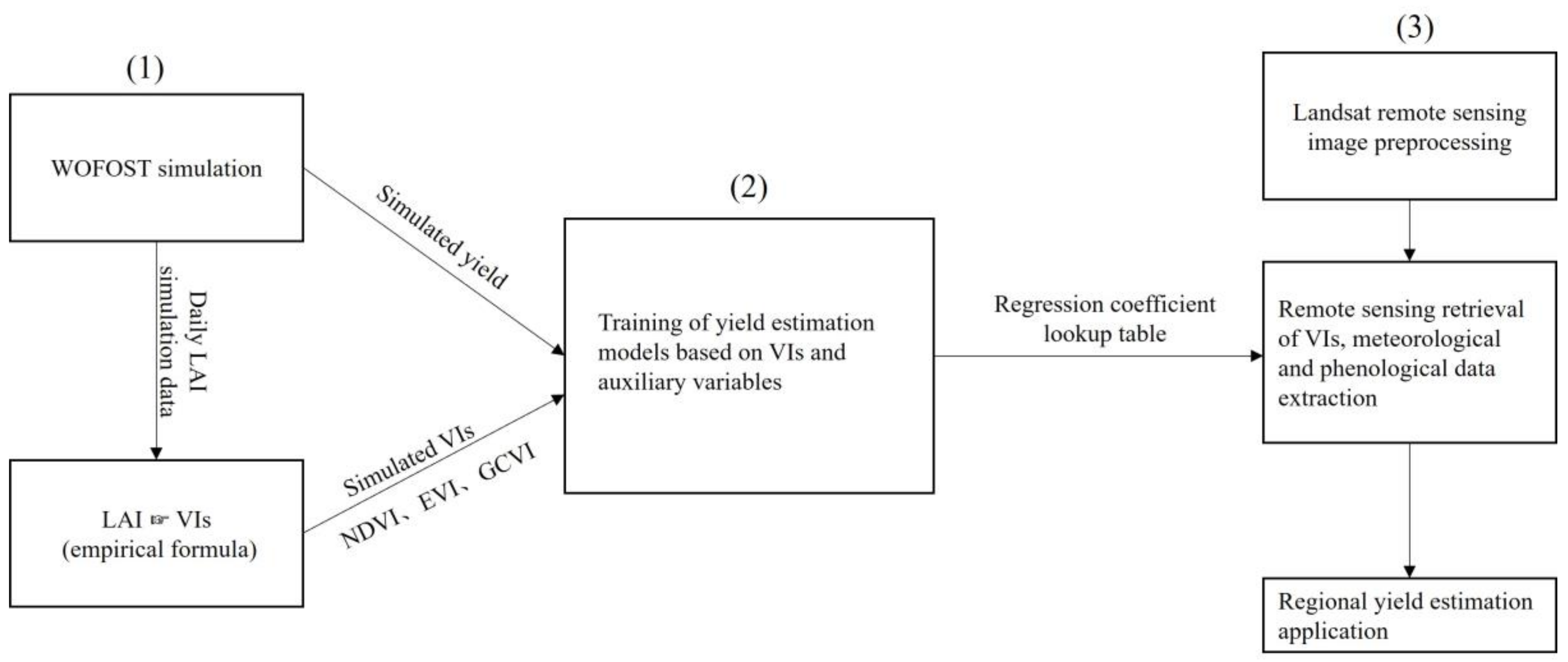
2.3.1. Application of the SCYM Method Framework

The SCYM method leverages crop growth models to simulate crop physiological characteristics and their responses to varying weather conditions and agricultural management practices. It also takes full advantage of the GEE cloud platform’s capability to process vast amounts of historical remote sensing data quickly. Compared to other empirical models, SCYM uses readily accessible data and does not require actual yield data for model calibration. The workflow of the SCYM method can be summarized as follows: (1) crop data simulation based on WOFOST; (2) yield estimation model training; and (3) pixel-scale yield mapping based on the estimation model [24] (Figure 2).

In this study, we applied the SCYM method framework as follows: (1) We used a fully parameterized crop model WOFOST to generate sample data for training yield estimation models, producing daily Leaf Area Index (LAI) and yield data for each station and each year; (2) We converted the LAI data into three simulated vegetation indices using empirical formulas, and constructed yield estimation models with different ML methods to compare the contributions of different indices and ML methods; and (3) We applied the best variable combination across the entire study area to achieve pixel-level yield mapping.

2.3.2. Crop Growth Data Simulation

In this study, the WOFOST model was chosen to simulate crop growth. Developed by Wageningen University, the WOFOST model is a process-based dynamic mechanistic model that simulates crop growth dynamics on a daily time step under specific climatic and environmental conditions [48]. The model has been successfully applied in the NCP, particularly for winter wheat, with extensive validation. The parameterization and calibration of the WOFOST model based on AMS in the NCP are described in detail in previously published works by our research group [9].

The localized WOFOST model was run at 41 AMS sites across the NCP, as shown in Figure 1. To ensure stable model outputs, simulations started in 1990, and data from 2001 to 2015 were used, generating 615 crop simulation records under diverse growth conditions, including soil, climate, crop variety, and management practices. Each simulation outputted daily time series data of crop biophysical characteristics, including biomass, final yield, and LAI. The simulated LAI time series data were converted to vegetation index time series using empirical formulas [49], as shown in Equations (4)–(6), as follows:

$$\mathrm{N}\mathrm{D}\mathrm{V}\mathrm{I}=0.435+0.491\times (1-{\mathrm{e}}^{-0.801\times \mathrm{L}\mathrm{A}\mathrm{I}})$$

(4)

$$\mathrm{E}\mathrm{V}\mathrm{I}=0.173+0.554\times (1-{\mathrm{e}}^{-0.656\times \mathrm{L}\mathrm{A}\mathrm{I}})$$

(5)

$$\mathrm{G}\mathrm{C}\mathrm{V}\mathrm{I}=0.992+9.201\times (1-{\mathrm{e}}^{-0.189\times \mathrm{L}\mathrm{A}\mathrm{I}})$$

(6)

Figure 3 shows the time series of simulated LAI and the corresponding derived vegetation indices (GCVI, NDVI, EVI) for a selected site and year. This figure illustrates the temporal dynamics of winter wheat growth, with LAI peaking during the key growth stages, and the vegetation indices responding accordingly. The close relationship between LAI and the vegetation indices is evident, providing valuable insights into the growth patterns of winter wheat and the potential for using these indices in yield estimation models.

2.3.3. Model Training and Evaluation

The simulated vegetation indices and corresponding simulated yield data were used to train the yield estimation models. Additional auxiliary variables (including meteorological data and key phenological stage data) were incorporated into the models to evaluate their contributions to yield estimation. The performance of ordinary linear regression models and machine learning models in constructing yield models was also compared. The yield estimation model is formulated as follows:

$$Y=f({VI}_d,W,Phe)$$

(7)

where $Y$ represents yield, $W$ denotes a vector of meteorological variables (e.g., temperature, precipitation, solar radiation), $Phe$ indicates phenological information (e.g., total days of the growing season, days from greening to heading, days from heading to maturity, proportion of reproductive growth period), and ${VI}_d$ represents the vector of vegetation index values (NDVI, EVI, GCVI) observed on a specific combination of dates $d$. The data distribution characteristics of meteorological and phenological variables are presented in

Table 1. Descriptive statistical analysis of meteorological and phenological variables applied in yield estimation model training.

	precip a	sr b	tmean c	tmax d	t_key e	t_percent f
	mm	W/m2	°C	°C	days
mean	175.46	231.12	14.89	30.69	44.14	0.32
min	66	187.95	9.4	22.8	28	0.16
max	482	251	17.53	35.6	60	0.59
std	69.17	10.84	1.41	2.26	7.67	0.10

^a precip means cumulative rainfall during the growing season; ^b sr means average solar radiation during the growing season; ^c tmean means average temperature during the growing season; ^d tmax means average maximum temperature from heading to maturity; ^e t_key means the duration from heading to maturity; ^f t_percent means the ratio of t_key to the entire growth period.

.

The explicit dependence on the date combination $d$ is a crucial aspect of the SCYM method, as $d$ corresponds to the dates of remote sensing image acquisition. Due to cloud cover, even nearby pixels may be observed on different dates. Lobell et al. divided the crop growing season into two stages, with $d$ corresponding to two observation windows. Considering the 16-day revisit period of Landsat imagery, this study also selected two observation windows: day of year (DOY) 101–130 and 131–160, resulting in 900 possible date combinations.

Three representative regression methods were chosen to train the yield estimation models: traditional ordinary least squares (OLS) and two powerful machine learning models, random forest (RF) and Light Gradient Boosting Machine (LightGBM). OLS minimizes the sum of squared errors to find the best fit, assuming a linear relationship between dependent and independent variables, normal distribution, and no multicollinearity. LightGBM, released by Microsoft in 2017, is an implementation of gradient boosting decision trees (GBDT) with improvements in performance and computational time [50]. RF is based on the concept of bagging, randomly selecting features to construct trees, and averaging the predictions of all trees, effectively addressing bias and variance components [3,51].

In this study, we implemented a robust approach to ensure both the effectiveness and generalization ability of the models used for yield prediction. Our dataset comprised 615 sample datasets, collected from 41 sites across the study area from 2001 to 2015. These samples were organized based on a combination of observation dates, specifically selecting 30-day periods from both the early and late stages of the growing season. This approach resulted in a total of 900 observation combinations, encompassing a wide range of environmental and climatic conditions.

The dataset was divided into training and test sets, with 70% of the data used for training and the remaining 30% reserved for testing. To optimize the model parameters, we employed 10-fold cross-validation and grid search techniques exclusively on the training set. The optimized models were then tested on the independent test set, and their performance was evaluated using the coefficient of determination (R²) and root-mean-square error (RMSE), as follows:

$${\mathrm{R}}^2=1-{\sum }_{i=1}^n{\left(y_i-{\widehat{y}}_i\right)}^2/{\sum }_{i=1}^n{\left(y_i-\overline{y}\right)}^2$$

(8)

$$\mathrm{RMSE}=\sqrt{{\displaystyle \frac{1}{n}}{\sum }_{i=1}^n{(y_i-{\widehat{y}}_i)}^2}$$

(9)

where n represents the number of total validation samples (n = 185), $\overline{y}$ represents the average value of simulated yield ouput by WOFOST, and ${\widehat{y}}_i$ represents the average value of estimated yield.

To assess the generalization ability of the models, we conducted a comprehensive evaluation process. The entire training and testing procedure was repeated 100 times to mitigate the uncertainty in the predicted R² values. By averaging the R² values across these iterations, we were able to obtain a reliable measure of each model’s performance. Furthermore, the model was applied at the grid scale to predict historical winter wheat yield data, and its accuracy was validated at the county scale. This approach demonstrated the model’s ability to generalize across different temporal and spatial conditions.

2.3.4. Experimental Design

To systematically address the three research questions, the following experimental schemes were designed:

(1)

VI Only: This experiment focuses on modeling yield estimation using only vegetation indices (GCVI, NDVI, EVI). It is intended to evaluate the effectiveness of different VIs in predicting winter wheat yield at the field scale;

(2)

Weather Only: In this experiment, the model is trained using only meteorological variables. The goal is to assess how meteorological factors alone contribute to yield estimation accuracy;

(3)

VI + Weather: This experiment combines vegetation indices with meteorological variables in the model. It explores the potential improvement in yield estimation accuracy when both VIs and weather data are used together;

(4)

VI + Phe: Here, the model uses both vegetation indices and phenological variables. The experiment aims to determine the added value of phenological information in improving yield estimation accuracy;

(5)

VI + Weather + Phe: This comprehensive experiment incorporates vegetation indices, meteorological variables, and phenological variables into the model. It evaluates the optimal combination of these inputs for enhancing yield prediction accuracy.

Explanation of experimental schemes: Experiment 1 compares the performance of the three indices. Experiments 1 to 3 assess the contributions of meteorological variables and vegetation indices to the yield estimation model. Experiments 3 to 5 evaluate the contribution of phenological information to the yield estimation model. All the above experimental schemes were implemented using three different machine learning methods. This approach allows for a comparative evaluation of the performance of each method in yield estimation under varying input conditions.

3. Results

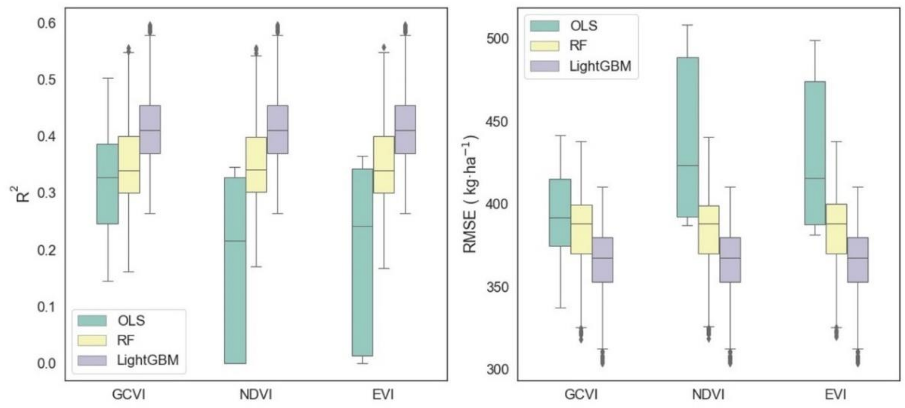
3.1. Accuracy of the Prediction Models with Only Vegetation Index

To compare the performance of different vegetation indices in winter wheat yield estimation models, we initially trained the models using only the vegetation index variables, evaluating their performance using R² and RMSE. As shown in Figure 4, depending on the choice of vegetation index and model, about 15–43% of the variations in winter wheat yield could be explained. In the multiple linear regression model, GCVI performed the best (R² = 0.31; RMSE = 396 kg·ha⁻¹), followed by EVI (R² = 0.18; RMSE = 430 kg·ha⁻¹), and NDVI performed the worst (R² = 0.15; RMSE = 438 kg·ha⁻¹). The R² values here refer to the average of the 900 observation date combinations, not to the highest value.

3.2. Contribution and Importance of Weather Variables and Phenological Metrics

The linear yield estimation model using only meteorological variables achieved an R² of 0.23, with an RMSE of 411 kg·ha⁻¹, which is lower than the accuracy achieved using only GCVI (R² = 0.31; RMSE = 396 kg·ha⁻¹). Similar patterns were observed in the RF and LightGBM methods, indicating that GCVI explains winter wheat yield variations better than meteorological variables. Moreover, the improvement in prediction accuracy for meteorological variables using machine learning methods (RF and LightGBM) over multiple linear regression (OLS) was only 0.03. In contrast, improvements for the GCVI non-linear models over linear models ranged from 0.04 to 0.11, suggesting that the relationship between meteorological variables and yield is more linear compared to vegetation indices.

To verify the impact of high-temperature stress from heading to maturity on final yield, the average maximum temperature variable (tmax) was excluded from the meteorological variables and the yield estimation was re-modeled. The changes in R² before and after this exclusion were compared to assess its contribution to yield variations (

Table 2. Model performance using different vegetation indices, different combinations of variables, and different methods.

		OLS		RF		LightGBM
		R2	RMSE	R2	RMSE	R2	RMSE
Vis a only	GCVI	0.31	396	0.35	384	0.42	365
	NDVI	0.15	438	0.35	384	0.42	365
	EVI	0.18	430	0.35	384	0.42	365
Climate b only		0.23	411	0.26	402	0.26	401
VIs + Climate	GCVI	0.51	326	0.57	307	0.57	307
	NDVI	0.44	349	0.57	307	0.57	307
	EVI	0.46	343	0.57	307	0.57	307
VIs + Phe c	GCVI	0.39	362	0.40	359	0.45	345
	NDVI	0.23	407	0.40	359	0.45	345
	EVI	0.26	397	0.40	359	0.45	345
VIs + Climate + Phe	GCVI	0.56	312	0.60	295	0.58	301
	NDVI	0.46	343	0.60	295	0.58	301
	EVI	0.49	335	0.60	295	0.58	301

^a VIs including NDVI, EVI, GCVI; ^b Climate including all climate variables; ^c Phe represents the combination of phenological variables.

and

Table 3. Contribution of meteorological variables to yield estimation model.

	OLS		RF		LightGBM
	R2	RMSE	R2	RMSE	R2	RMSE
Climate’ a only	0.00	467	0.14	436	0.16	431
GCVI + Climate’	0.44	351	0.55	315	0.55	317
GCVI + Climate’ + Phe	0.51	328	0.60	296	0.58	304

^a Climate’ means that the meteorological variable set excludes the mean maximum temperature (tmax) variable after the heading stage of winter wheat.

). It was found that the average maximum temperature from heading to maturity, as shown in Table 2 and Table 3, contributed significantly to the final yield, especially for the linear models (R² increased by 0.05–0.23). In the linear model using only meteorological variables, other meteorological variables contributed negligibly to the final yield, indicating a weak linear relationship between other meteorological variables and the final yield (Figure 5). The contribution of the average maximum temperature to yield variations (R²) decreased with the use of non-linear models and the inclusion of more variables. Similarly, the inclusion of phenological variables effectively improved model accuracy (Table 2), with an 8% increase in R² for linear models compared to the models using only GCVI. Still, the contribution to non-linear models was relatively smaller (5% and 3% for RF and LightGBM, respectively).

To assess the impact of climatic and phenological variables on yield estimation accuracy, we compared the performance of different model configurations. The inclusion of climatic variables (e.g., GCVI + climate) provided a notable improvement in accuracy over using vegetation indices alone. However, when phenological information was added to the model that already included climatic variables (GCVI + climate + Phe), the accuracy increased by only 1% to 5% (Table 2). This small improvement suggests that the phenological variables’ contribution was reduced by approximately 3% compared to their impact when climatic variables were not considered. This overlap indicates that some of the phenological information may be redundant or already captured by the climatic variables.

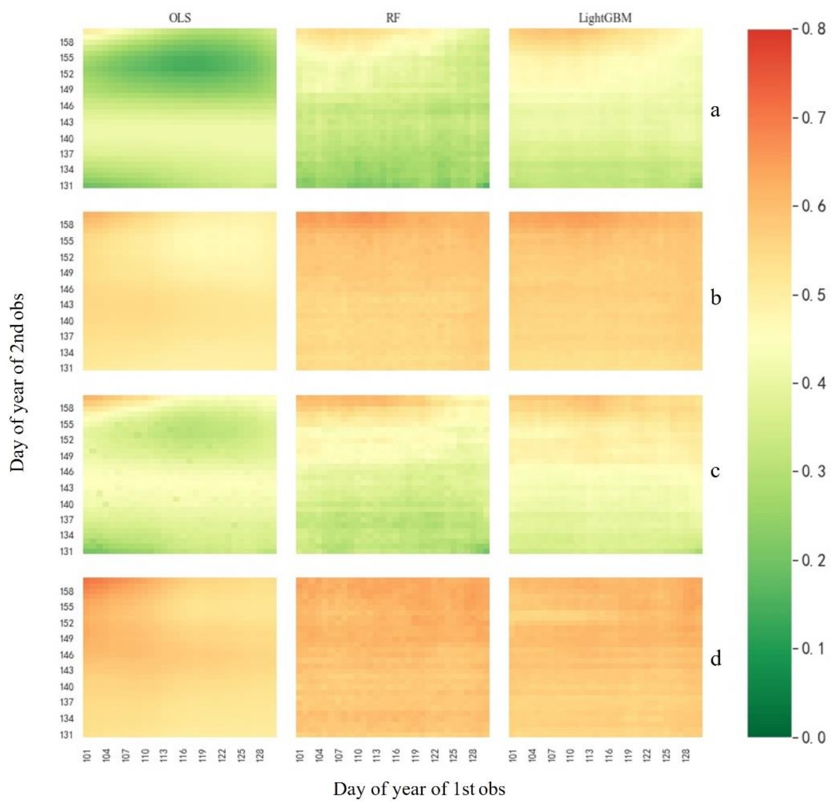
3.3. Impact of Vegetation Index Observation Dates on Yield Estimation Models

Furthermore, this study analyzed the effect of vegetation index observation dates on winter wheat yield estimation models. The results showed that when only vegetation indices were used for yield estimation, the model accuracy significantly depended on the choice of observation dates. As shown in Figure 6, for multiple linear regression, the accuracy of the model relying solely on GCVI was highly dependent on the observation dates, with the late growing season observations concentrated between DOY 135 and 145 (approximately 15–25 May) and the early growing season observations also showing higher accuracy towards the later period (DOY 121–130). By May, most winter wheat fields in the NCP had reached, or were close to, the peak vegetation index (Figure 2), indicating that the peak vegetation index values contributed the most to model accuracy, which is consistent with the results shown in previous studies [26].

However, with the addition of more variables and the introduction of more complex machine learning methods, this dependence on observation dates gradually weakened. Comparing Figure 6a,b, the linear yield estimation model exhibited better prediction accuracy over a broader range of observation dates with the inclusion of meteorological variables. For non-linear models (RF and LightGBM), the effect of vegetation index observation dates on yield estimation models was almost eliminated, achieving high prediction accuracy with any combination of observation dates.

Compared to yield estimation models relying solely on vegetation indices, the inclusion of phenological metrics improved the overall performance of the prediction models. Still, the requirement for observation dates did not change significantly (Figure 6a,c). The combined models of vegetation indices, meteorological variables, and phenological metrics achieved the highest accuracy, yielding satisfactory results across all combinations of observation dates (Figure 6d).

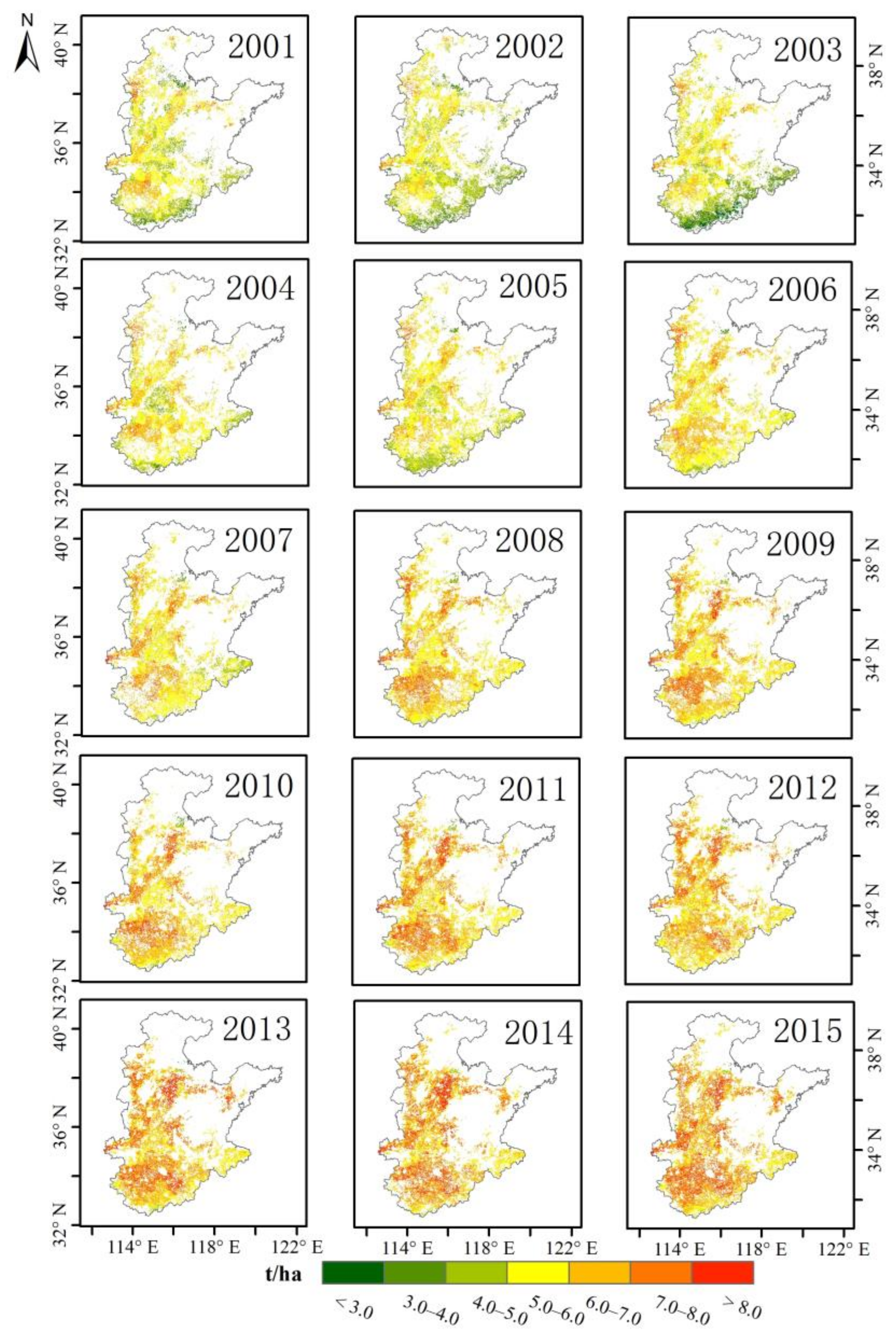
3.4. Winter Wheat Yield Spatial Mapping and Accuracy Evaluation

The regression models for different observation date combinations were stored as regression coefficient lookup tables. Using the GCVI data derived from Landsat 7, TerraClimate climate variable data, locally uploaded phenological variable datasets, and winter wheat spatial distribution datasets on the GEE platform, we calculated pixel-level winter wheat yield estimates for the years 2001–2015. The results are shown in Figure 7.

County administrative units averaged the simulated winter wheat yield data obtained through the SCYM method to estimate county-level winter wheat yields. These estimates were compared with county-level winter wheat yield data collected from statistical records (only comparing the results from 2001–2011 due to significant data gaps in county-level yield statistics after 2012) to evaluate the accuracy of the SCYM-based winter wheat yield simulation in the NCP. The results showed a significant positive correlation between simulated yields and statistical yields in all comparison years (R² ≥ 0.67, up to 0.89, RMSE ≤ 733 kg·ha⁻¹), as shown in Figure 8. This represents a significant improvement in accuracy compared to the SCYM method applied by George et al. (2017) in the winter wheat-growing regions of India (R² ≥ 0.45) [26]. Cao et al. (2020) attempted to predict winter wheat yields in the NCP at the county level by integrating multi-source data, including monthly climate data, satellite data (i.e., vegetation index datasets), and socioeconomic factors [51]. Their results showed that three machine learning models (ridge regression, random forest, and LightGBM) achieved the highest accuracy when all input data were combined (R²: 0.68–0.75). Compared to this study, the county-level yield estimation accuracy is similar but slightly lower. In addition, unlike the county-level results of Cao et al., our study provides richer spatial information on yields at a similar accuracy level (Figure 7).

4. Discussion

4.1. Comparison of the Performance of Vegetation Indices in Yield Estimation

In this study, we found that in linear models, GCVI performed the best (including diverse combinations of variables), EVI ranked second place, and NDVI ranked last, illustrating that GCVI is more suitable for predicting the yield of winter wheat. Despite being the most widely used indicator for crop growth monitoring and yield estimation due to its high correlation with crop vigor and aboveground biomass, NDVI tends to saturate at moderate-to-high LAI values (LAI > 3) [52,53]. The EVI was developed to minimize the influence of soil background reflectance and atmospheric conditions, thus improving sensitivity to high LAI values. However, both NDVI and EVI primarily reflect leaf structure and greenness rather than environmental stress information. The GCVI estimates leaf chlorophyll content, which reflects the physiological state of plants. As chlorophyll content decreases under stress, GCVI serves as a good indicator of plant health [54].

In non-linear models (RF and LightGBM), the three vegetation indices showed highly similar performances in explaining yield variations (Figure 4), with the differences in R² and RMSE being less than 0.001. Previous studies have also found similar results, where different vegetation indices have comparable explanatory power for yield variations in machine learning models [3]. This consistency can be attributed to the inherent similarity in the non-linear relationships between vegetation indices and crop biomass yields. Additionally, all three vegetation indices were derived from the same LAI data using empirical relationships (Equations (4)–(6)), which may contribute to the observed similarity. Further validation through actual observation experiments is needed to investigate the specific reasons. Overall, GCVI is more suitable for winter wheat yield estimation compared to NDVI and EVI.

4.2. Comparing the Performances of OLS and ML Methods in Predicting Crop Yield

The results indicate that non-linear machine learning methods (RF and LightGBM) outperform linear methods (OLS) in yield prediction, consistent with previous studies. For various combinations of variables, machine learning methods performed better than multiple linear regression methods (Table 2). When considering only meteorological variables, adding GCVI observation combinations to non-linear models improved R² more significantly (0.31) than in linear models (0.29), indicating that vegetation indices contribute more non-linearly to crop yield. Conversely, when only GCVI observation combinations were used, adding meteorological variables improved the average R² of non-linear models less than that of the linear models, suggesting a more linear relationship between meteorological variables and crop yield (Figure 5) [55].

4.3. Effects of Image Observation Date on Yield Estimation

The previous results demonstrated that yield estimation models relying solely on GCVI observation combinations were highly dependent on observation dates, and that this dependence gradually decreased with the addition of more input variables. To further investigate the effect of vegetation index observation dates on final yield estimation, we repeated the experiments using single-phase GCVI observations. The results showed that peak vegetation indices had the highest correlation with crop yields, providing more information related to biotic or abiotic factors [56,57]. As shown in Figure 9a, using single-phase GCVI to train yield estimation models day by day, all three methods achieved the highest accuracy of around DOY 140. Since the climate and phenological variables selected in this study present comprehensive information for the entire growing season, their inclusion compensated for the limitations of vegetation indices in reflecting the instantaneous growth status of crops, thereby reducing the dependence on vegetation index observation dates. Thus, as shown in Figure 9b, with the addition of climate and phenological variables, the suitable observation dates for single-phase GCVI extended from around DOY 140 to DOY 120–145 for all methods.

In addition, our model shows promise for real-time yield forecasting. As shown in Figure 9a, the model achieves the highest accuracy for winter wheat yield estimation, of around DOY 140, when using vegetation indices alone. From this point onward, it is feasible to use real-time remote sensing data to predict winter wheat yields. Furthermore, by integrating agricultural meteorological forecast data, the accuracy of these predictions can be enhanced (Figure 9b). This real-time application could prove to be invaluable for dynamic agricultural decision-making, including irrigation scheduling, pest management, and harvest planning. The ability to transition from a research tool to a real-time management tool could significantly improve the efficiency and effectiveness of agricultural practices, underscoring the practical value of our model.

4.4. Uncertainties and Outlook

Inevitably, there are uncertainties in the study results. First, the SCYM method assumes that crop growth models can accurately simulate final yield and LAI. Although the parameter-adjusted WOFOST model can more accurately simulate crop yield and has been widely validated, there is less research on LAI. For example, some studies have found that the crop model tends to slightly overestimate LAI [58], a phenomenon also observed in this study. Second, crop models focus on yield under water and nutrient limitations and are less adaptable to pests, diseases, and extreme weather. Therefore, empirical models based on these simulations cannot also evaluate crop yields under extreme conditions (adverse weather or biological stress). In this study, we introduced average maximum temperature and phenological information from heading to maturity to improve the model’s adaptability to extreme conditions. Third, the empirical relationship-based LAI inversion process for vegetation indices is also a major source of errors. Additionally, obtaining multi-source data, such as climate and phenological variables, inherently involves errors that may affect the results. Finally, in terms of climate variables, this study only selected comprehensive information covering the winter wheat growing season, making it difficult to avoid the possibility of omitting essential variables. Future studies will screen climate variables monthly. Similarly, the selection of phenological indicators also requires further exploration [59].

In addition to the uncertainties discussed, there is substantial potential for improving the presented methodology by incorporating additional remote sensing data sources. For example, synthetic aperture radar (SAR) data can be utilized to derive LAI with high accuracy by coupling it with canopy radiative transfer models [60]. This approach could eliminate the need for empirical conversions between vegetation indices and LAI, reducing the associated uncertainties. Furthermore, SAR’s resilience to atmospheric conditions and its ability to operate under all weather conditions make it a highly reliable data source. Looking ahead, we plan to integrate SAR data, along with other promising remote sensing technologies such as solar-induced chlorophyll fluorescence (SIF) and near-infrared reflectance of vegetation (NIRv) [32], into our methodology. These additions could significantly enhance the accuracy and robustness of crop yield estimation models by providing more direct and detailed insights into crop health and development.

Although this study has many limitations, it provides an operational, scalable, flexible, and multiscale adaptive remote sensing yield estimation modeling method based on the SCYM method. It offers new ideas for determining input variable combinations and method selection.

5. Conclusions

This study integrated vegetation indices, meteorological, and phenological information to improve the accuracy and efficiency of crop yield evaluation using machine learning methods. We evaluated the performance of three vegetation indices (NDVI, EVI, and GCVI) and three machine learning methods (OLS, RF, and LightGBM) in winter wheat yield modeling. The results showed that GCVI performed best in predicting winter wheat yield with linear models (OLS), followed by EVI, and that NDVI performed the worst. Non-linear machine learning methods (RF and LightGBM) significantly outperformed linear models (OLS), with LightGBM performing the best, followed by RF. The combination of vegetation indices, meteorological, and phenological information achieved the best performance in winter wheat yield estimation, obtaining high accuracy across all observation date combinations. Our study found that the average maximum temperature from heading to maturity (tmax) significantly contributed to improving yield estimation accuracy. The addition of phenological information also enhanced yield estimation accuracy.

Due to various factors, most countries or regions lack sufficient long-term continuous ground crop observation data, which are essential for traditional empirical model-based remote sensing yield estimation. The SCYM method, based on crop model-calibrated empirical models, provides a pivotal approach to addressing this issue. Therefore, this study proposes a framework for regional remote sensing yield estimation based on the SCYM method, which includes index selection, modeling method comparison, and rapid screening and optimization of input variable combinations. This framework does not require actual ground yield data for model training, making it easily applicable to other regions and other crops.

References

1. Shiferaw, B.; Smale, M.; Braun, H.-J.; Duveiller, E.; Reynolds, M.; Muricho, G. Crops that feed the world 10. Past successes and future challenges to the role played by wheat in global food security. Food Secur. 2013, 5, 291–317. [Google Scholar] [CrossRef]
2. Sun, H.; Wang, Y.; Wang, L. Impact of climate change on wheat production in China. Eur. J. Agron. 2024, 153, 127066. [Google Scholar] [CrossRef]
3. Zhang, L.; Zhang, Z.; Luo, Y.; Cao, J.; Tao, F. Combining optical, fluorescence, thermal satellite, and environmental data to predict county-level maize yield in China using machine learning approaches. Remote Sens. 2019, 12, 21. [Google Scholar] [CrossRef]
4. Van Klompenburg, T.; Kassahun, A.; Catal, C. Crop yield prediction using machine learning: A systematic literature review. Comput. Electron. Agric. 2020, 177, 105709. [Google Scholar] [CrossRef]
5. Basso, B.; Liu, L. Seasonal crop yield forecast: Methods, applications, and accuracies. Adv. Agron. 2019, 154, 201–255. [Google Scholar]
6. Prasad, A.K.; Chai, L.; Singh, R.P.; Kafatos, M. Crop yield estimation model for Iowa using remote sensing and surface parameters. Int. J. Appl. Earth Obs. Geoinf. 2006, 8, 26–33. [Google Scholar] [CrossRef]
7. Lobell, D.B.; Asseng, S. Comparing estimates of climate change impacts from process-based and statistical crop models. Environ. Res. Lett. 2017, 12, 015001. [Google Scholar] [CrossRef]
8. Sakamoto, T. Incorporating environmental variables into a MODIS-based crop yield estimation method for United States corn and soybeans through the use of a random forest regression algorithm. ISPRS J. Photogramm. Remote Sens. 2020, 160, 208–228. [Google Scholar] [CrossRef]
9. Huang, H.; Huang, J.; Li, X.; Zhuo, W.; Wu, Y.; Niu, Q.; Su, W.; Yuan, W. A dataset of winter wheat aboveground biomass in China during 2007–2015 based on data assimilation. Sci. Data 2022, 9, 200. [Google Scholar] [CrossRef]
10. Shahhosseini, M.; Hu, G.; Huber, I.; Archontoulis, S.V. Coupling machine learning and crop modeling improves crop yield prediction in the US Corn Belt. Sci. Rep. 2021, 11, 1606. [Google Scholar] [CrossRef]
11. Manivasagam, V.; Rozenstein, O. Practices for upscaling crop simulation models from field scale to large regions. Comput. Electron. Agric. 2020, 175, 105554. [Google Scholar] [CrossRef]
12. Peng, B.; Guan, K.; Tang, J.; Ainsworth, E.A.; Asseng, S.; Bernacchi, C.J.; Cooper, M.; Delucia, E.H.; Elliott, J.W.; Ewert, F. Towards a multiscale crop modelling framework for climate change adaptation assessment. Nat. Plants 2020, 6, 338–348. [Google Scholar] [CrossRef]
13. Báez-González, A.D.; Chen, P.y.; Tiscareño-López, M.; Srinivasan, R. Using satellite and field data with crop growth modeling to monitor and estimate corn yield in Mexico. Crop Sci. 2002, 42, 1943–1949. [Google Scholar] [CrossRef]
14. Shanahan, J.F.; Schepers, J.S.; Francis, D.D.; Varvel, G.E.; Wilhelm, W.W.; Tringe, J.M.; Schlemmer, M.R.; Major, D.J. Use of remote-sensing imagery to estimate corn grain yield. Agron. J. 2001, 93, 583–589. [Google Scholar] [CrossRef]
15. Dias, H.B.; Sentelhas, P.C. Evaluation of three sugarcane simulation models and their ensemble for yield estimation in commercially managed fields. Field Crops Res. 2017, 213, 174–185. [Google Scholar] [CrossRef]
16. Kephe, P.N.; Ayisi, K.K.; Petja, B.M. Challenges and opportunities in crop simulation modelling under seasonal and projected climate change scenarios for crop production in South Africa. Agric. Food Secur. 2021, 10, 1–24. [Google Scholar] [CrossRef]
17. Appiah, M.; Bracho-Mujica, G.; Svane, S.; Styczen, M.; Kersebaum, K.C.; Rötter, R.P. The impact of high quality field data on crop model calibration. In Proceedings of the EGU General Assembly Conference 2022, Vienna, Austria, 23–27 May 2022. [Google Scholar] [CrossRef]
18. Schauberger, B.; Jägermeyr, J.; Gornott, C. A systematic review of local to regional yield forecasting approaches and frequently used data resources. Eur. J. Agron. 2020, 120, 126153. [Google Scholar] [CrossRef]
19. Lobell, D.B.; Burke, M.B. On the use of statistical models to predict crop yield responses to climate change. Agric. For. Meteorol. 2010, 150, 1443–1452. [Google Scholar] [CrossRef]
20. Li, Y.; Guan, K.; Yu, A.; Peng, B.; Zhao, L.; Li, B.; Peng, J. Toward building a transparent statistical model for improving crop yield prediction: Modeling rainfed corn in the US. Field Crops Res. 2019, 234, 55–65. [Google Scholar] [CrossRef]
21. Clevers, J. A simplified approach for yield prediction of sugar beet based on optical remote sensing data. Remote Sens. Environ. 1997, 61, 221–228. [Google Scholar] [CrossRef]
22. Sehgal, V.; Sastri, C.; Kalra, N.; Dadhwal, V. Farm-level yield mapping for precision crop management by linking remote sensing inputs and a crop simulation model. J. Indian Soc. Remote Sens. 2005, 33, 131–136. [Google Scholar] [CrossRef]
23. Sibley, A.M.; Grassini, P.; Thomas, N.E.; Cassman, K.G.; Lobell, D.B. Testing remote sensing approaches for assessing yield variability among maize fields. Agron. J. 2014, 106, 24–32. [Google Scholar] [CrossRef]
24. Lobell, D.B.; Thau, D.; Seifert, C.; Engle, E.; Little, B. A scalable satellite-based crop yield mapper. Remote Sens. Environ. 2015, 164, 324–333. [Google Scholar] [CrossRef]
25. Jin, Z.; Azzari, G.; Lobell, D.B. Improving the accuracy of satellite-based high-resolution yield estimation: A test of multiple scalable approaches. Agric. For. Meteorol. 2017, 247, 207–220. [Google Scholar] [CrossRef]
26. Azzari, G.; Jain, M.; Lobell, D.B. Towards fine resolution global maps of crop yields: Testing multiple methods and satellites in three countries. Remote Sens. Environ. 2017, 202, 129–141. [Google Scholar] [CrossRef]
27. Deines, J.M.; Patel, R.; Liang, S.-Z.; Dado, W.; Lobell, D.B. A million kernels of truth: Insights into scalable satellite maize yield mapping and yield gap analysis from an extensive ground dataset in the US Corn Belt. Remote Sens. Environ. 2021, 253, 112174. [Google Scholar] [CrossRef]
28. Waldner, F.; Horan, H.; Chen, Y.; Hochman, Z. High temporal resolution of leaf area data improves empirical estimation of grain yield. Sci. Rep. 2019, 9, 15714. [Google Scholar] [CrossRef]
29. Zhao, Y.; Xiao, D.; Bai, H. The simultaneous prediction of yield and maturity date for wheat–maize by combining satellite images with crop model. J. Sci. Food Agric. 2024. online. [Google Scholar] [CrossRef] [PubMed]
30. Jain, M.; Singh, B.; Srivastava, A.; Malik, R.K.; McDonald, A.; Lobell, D.B. Using satellite data to identify the causes of and potential solutions for yield gaps in India’s Wheat Belt. Environ. Res. Lett. 2017, 12, 094011. [Google Scholar] [CrossRef]
31. Seifert, C.A.; Azzari, G.; Lobell, D.B. Satellite detection of cover crops and their effects on crop yield in the Midwestern United States. Environ. Res. Lett. 2018, 13, 064033. [Google Scholar] [CrossRef]
32. Zeng, Y.; Hao, D.; Huete, A.; Dechant, B.; Berry, J.; Chen, J.M.; Joiner, J.; Frankenberg, C.; Bond-Lamberty, B.; Ryu, Y. Optical vegetation indices for monitoring terrestrial ecosystems globally. Nat. Rev. Earth Environ. 2022, 3, 477–493. [Google Scholar] [CrossRef]
33. Wang, Q.; Adiku, S.; Tenhunen, J.; Granier, A. On the relationship of NDVI with leaf area index in a deciduous forest site. Remote Sens. Environ. 2005, 94, 244–255. [Google Scholar] [CrossRef]
34. Zhang, L.; Zhang, Z.; Luo, Y.; Cao, J.; Xie, R.; Li, S. Integrating satellite-derived climatic and vegetation indices to predict smallholder maize yield using deep learning. Agric. For. Meteorol. 2021, 311, 108666. [Google Scholar] [CrossRef]
35. Shuai, G.; Basso, B. Subfield maize yield prediction improves when in-season crop water deficit is included in remote sensing imagery-based models. Remote Sens. Environ. 2022, 272, 112938. [Google Scholar] [CrossRef]
36. Zhu, X.; Guo, R.; Liu, T.; Xu, K. Crop yield prediction based on agrometeorological indexes and remote sensing data. Remote Sens. 2021, 13, 2016. [Google Scholar] [CrossRef]
37. Han, D.; Wang, P.; Tansey, K.; Zhang, S.; Tian, H.; Zhang, Y.; Li, H. Improving wheat yield estimates by integrating a remotely sensed drought monitoring index into the simple algorithm for yield estimate model. IEEE J. Sel. Top. Appl. Earth Obs. Remote Sens. 2021, 14, 10383–10394. [Google Scholar] [CrossRef]
38. Sakamoto, T.; Gitelson, A.A.; Arkebauer, T.J. MODIS-based corn grain yield estimation model incorporating crop phenology information. Remote Sens. Environ. 2013, 131, 215–231. [Google Scholar] [CrossRef]
39. Li, S.; Sun, Z.; Zhang, X.; Zhu, W.; Li, Y. An improved threshold method to detect the phenology of winter wheat. In Proceedings of the 2018 7th International Conference on Agro-Geoinformatics (Agro-Geoinformatics), Hangzhou, China, 6–9 August 2018; pp. 1–5. [Google Scholar]
40. Cheng, E.; Zhang, B.; Peng, D.; Zhong, L.; Yu, L.; Liu, Y.; Xiao, C.; Li, C.; Li, X.; Chen, Y. Wheat yield estimation using remote sensing data based on machine learning approaches. Front. Plant Sci. 2022, 13, 1090970. [Google Scholar] [CrossRef] [PubMed]
41. Ashapure, A.; Jung, J.; Chang, A.; Oh, S.; Yeom, J.; Maeda, M.; Maeda, A.; Dube, N.; Landivar, J.; Hague, S. Developing a machine learning based cotton yield estimation framework using multi-temporal UAS data. ISPRS J. Photogramm. Remote Sens. 2020, 169, 180–194. [Google Scholar] [CrossRef]
42. Guo, H.; Li, M.; Wang, L.; Wang, Y.; Zang, X.; Zhao, X.; Wang, H.; Zhu, J. Evaluation of groundwater suitability for irrigation and drinking purposes in an agricultural region of the North China Plain. Water 2021, 13, 3426. [Google Scholar] [CrossRef]
43. Gorelick, N.; Hancher, M.; Dixon, M.; Ilyushchenko, S.; Thau, D.; Moore, R. Google Earth Engine: Planetary-scale geospatial analysis for everyone. Remote Sens. Environ. 2017, 202, 18–27. [Google Scholar] [CrossRef]
44. Balaghi, R.; Tychon, B.; Eerens, H.; Jlibene, M. Empirical regression models using NDVI, rainfall and temperature data for the early prediction of wheat grain yields in Morocco. Int. J. Appl. Earth Obs. Geoinf. 2008, 10, 438–452. [Google Scholar] [CrossRef]
45. Son, N.; Chen, C.; Chen, C.; Minh, V.; Trung, N. A comparative analysis of multitemporal MODIS EVI and NDVI data for large-scale rice yield estimation. Agric. For. Meteorol. 2014, 197, 52–64. [Google Scholar] [CrossRef]
46. Abatzoglou, J.T.; Dobrowski, S.Z.; Parks, S.A.; Hegewisch, K.C. TerraClimate, a high-resolution global dataset of monthly climate and climatic water balance from 1958–2015. Sci. Data 2018, 5, 1–12. [Google Scholar] [CrossRef] [PubMed]
47. Luo, Y.; Zhang, Z.; Li, Z.; Chen, Y.; Zhang, L.; Cao, J.; Tao, F. Identifying the spatiotemporal changes of annual harvesting areas for three staple crops in China by integrating multi-data sources. Environ. Res. Lett. 2020, 15, 074003. [Google Scholar] [CrossRef]
48. Van Diepen, C.v.; Wolf, J.v.; Van Keulen, H.; Rappoldt, C. WOFOST: A simulation model of crop production. Soil Use Manag. 1989, 5, 16–24. [Google Scholar] [CrossRef]
49. Tanaka, S.; Kawamura, K.; Maki, M.; Muramoto, Y.; Yoshida, K.; Akiyama, T. Spectral index for quantifying leaf area index of winter wheat by field hyperspectral measurements: A case study in Gifu Prefecture, Central Japan. Remote Sens. 2015, 7, 5329–5346. [Google Scholar] [CrossRef]
50. Ke, G.; Meng, Q.; Finley, T.; Wang, T.; Chen, W.; Ma, W.; Ye, Q.; Liu, T.-Y. LightGBM: A Highly Efficient Gradient Boosting Decision Tree. In Proceedings of the NIPS’17 31st International Conference on Neural Information Processing Systems, Long Beach, CA, USA, 4–9 December 2017; pp. 1–9. [Google Scholar]
51. Cao, J.; Zhang, Z.; Tao, F.; Zhang, L.; Luo, Y.; Han, J.; Li, Z. Identifying the contributions of multi-source data for winter wheat yield prediction in China. Remote Sens. 2020, 12, 750. [Google Scholar] [CrossRef]
52. Mutanga, O.; Skidmore, A.K. Narrow band vegetation indices overcome the saturation problem in biomass estimation. Int. J. Remote Sens. 2004, 25, 3999–4014. [Google Scholar] [CrossRef]
53. Delegido, J.; Verrelst, J.; Meza, C.; Rivera, J.; Alonso, L.; Moreno, J. A red-edge spectral index for remote sensing estimation of green LAI over agroecosystems. Eur. J. Agron. 2013, 46, 42–52. [Google Scholar] [CrossRef]
54. Kimm, H.; Guan, K.; Jiang, C.; Miao, G.; Wu, G.; Suyker, A.E.; Ainsworth, E.A.; Bernacchi, C.J.; Montes, C.M.; Berry, J.A. A physiological signal derived from sun-induced chlorophyll fluorescence quantifies crop physiological response to environmental stresses in the US Corn Belt. Environ. Res. Lett. 2021, 16, 124051. [Google Scholar] [CrossRef]
55. Lecerf, R.; Ceglar, A.; López-Lozano, R.; Van Der Velde, M.; Baruth, B. Assessing the information in crop model and meteorological indicators to forecast crop yield over Europe. Agric. Syst. 2019, 168, 191–202. [Google Scholar] [CrossRef]
56. Chen, Y.; Zhang, Z.; Tao, F.; Wang, P.; Wei, X. Spatio-temporal patterns of winter wheat yield potential and yield gap during the past three decades in North China. Field Crops Res. 2017, 206, 11–20. [Google Scholar] [CrossRef]
57. Zhang, Z.; Wang, P.; Chen, Y.; Song, X.; Wei, X.; Shi, P. Global warming over 1960–2009 did increase heat stress and reduce cold stress in the major rice-planting areas across China. Eur. J. Agron. 2014, 59, 49–56. [Google Scholar] [CrossRef]
58. Huang, J.; Sedano, F.; Huang, Y.; Ma, H.; Li, X.; Liang, S.; Tian, L.; Zhang, X.; Fan, J.; Wu, W. Assimilating a synthetic Kalman filter leaf area index series into the WOFOST model to improve regional winter wheat yield estimation. Agric. For. Meteorol. 2016, 216, 188–202. [Google Scholar] [CrossRef]
59. Zhu, P.; Jin, Z.; Zhuang, Q.; Ciais, P.; Bernacchi, C.; Wang, X.; Makowski, D.; Lobell, D. The important but weakening maize yield benefit of grain filling prolongation in the US Midwest. Glob. Change Biol. 2018, 24, 4718–4730. [Google Scholar] [CrossRef]
60. Wu, S.; Yang, P.; Ren, J.; Chen, Z.; Liu, C.; Li, H. Winter wheat LAI inversion considering morphological characteristics at different growth stages coupled with microwave scattering model and canopy simulation model. Remote Sens. Environ. 2020, 240, 111681. [Google Scholar] [CrossRef]
Figure 1. Location of the study area and distribution of agrometeorological stations.
Remotesensing 16 03217 g001
Figure 2. Flow chart of yield estimation based on SCYM method: (1) crop growth data simulation; (2) training of the yield estimation model; and (3) generation of pixel-level yield estimation results.
Remotesensing 16 03217 g002
Figure 3. Example of time series of simulated LAI and derived vegetation indices (GCVI, NDVI, EVI) for a selected site and year.
Remotesensing 16 03217 g003
Figure 4. Comparison of different vegetation indices for yield estimation of winter wheat.
Remotesensing 16 03217 g004
Figure 5. The relationship between meteorological variables and yield. yield represents simulated yield, precip represents cumulative rainfall during the growing season, sr represents average radiation during the growing season, tmean represents average temperature during the growing season, and tmax represents the average maximum temperature from heading to maturity, t_key represents the duration from heading to maturity.
Remotesensing 16 03217 g005
Figure 6. The model performances (R2) for the regression models are based on different variables and method combinations. Each grid cell shows model results for a specific combination of observation dates from the two windows. Specifically, horizontally represents different methods (OLS, RF, and LightGBM). Vertically, the combinations of other variables from (ad): (a) only GCVI input; (b) GCVI + climate variables; (c) GCVI + phenological metrics; and (d) GCVI + climate variables + phenological metrics.
Remotesensing 16 03217 g006
Figure 7. Spatial distribution map of winter wheat yield estimation by remote sensing in the North China Plain from 2001 to 2015 based on SCYM method.
Remotesensing 16 03217 g007
Figure 8. Verification of simulation accuracy of winter wheat yield in the North China Plain.
Remotesensing 16 03217 g008
Figure 9. Effect of single-phase GCVI observation date on yield estimation model R2: (a) only GCVI; and (b) GCVI + climate variable + phenological variable.
Remotesensing 16 03217 g009