Abstract
Determining the responses of non-photosynthetic vegetation (NPV) and photosynthetic vegetation (PV) communities to climate change is crucial in illustrating the sensitivity and sustainability of these ecosystems. In this study, we evaluated the accuracy of inverting NPV and PV using Landsat imagery with random forest (RF), backpropagation neural network (BPNN), and fully connected neural network (FCNN) models. Additionally, we inverted MODIS NPV and PV time-series data using spectral unmixing. Based on this, we analyzed the responses of NPV and PV to precipitation and drought across different ecological regions. The main conclusions are as follows: (1) In NPV remote sensing inversion, the softmax activation function demonstrates greater advantages over the ReLU activation function. Specifically, the use of the softmax function results in an approximate increase of 0.35 in the R2 value. (2) Compared with a five-layer FCNN with 128 neurons and a three-layer BPNN with 12 neurons, a random forest model with over 50 trees and 5 leaf nodes provides better inversion results for NPV and PV (R2_RF-NPV = 0.843, R2_RF-PV = 0.861). (3) Long-term drought or heavy rainfall events can affect the utilization of precipitation by NPV and PV. There is a high correlation between extreme precipitation events following prolonged drought and an increase in PV coverage. (4) Under long-term drought conditions, the vegetation in the study area responded to precipitation during the last winter and growing season. This study provides an illustration of the response of semi-arid ecosystems to drought and wetting events, thereby offering a data basis for the effect evaluation of afforestation projects.
1. Introduction
Arid and semi-arid ecosystems are more sensitive to climate change and have weaker resilience [1], which significantly impacts global carbon cycling and carbon stocks [2,3]. By using remote sensing techniques to detect vegetation cover and study its response to climate, the sensitivity of arid and semi-arid ecosystems to drought can be quantified on a spatial scale [4]. In arid and semi-arid ecological communities, above-ground vegetation can be classified into non-photosynthetic components (ground litter and vertical dead vegetation) and photosynthetic components [5,6]. Specifically, distinguishing between the photosynthetic and non-photosynthetic components of vegetation can enhance our understanding of the impacts of climate change on vegetation production and ecological functions [7].
Non-photosynthetic vegetation (NPV) is a crucial component in the material cycles and energy flows within ecosystems [8,9]. In arid and semi-arid ecosystems, the interaction between litter and sandy soils positively influences hydrological processes, the physical and chemical properties of the soil, nutrient cycling, and vegetation recovery [10,11,12]. Photosynthetic vegetation (PV), on the other hand, reflects the photosynthetic activity, productivity, and overall health of the ecosystem. It serves as an indicator of soil erosion risks in arid and semi-arid ecosystems [13,14,15]. Remote sensing is a well-established approach for deriving coverage of non-photosynthetic vegetation (NPV) and photosynthetic vegetation (PV) [16,17]. Utilizing remote sensing to estimate the spatiotemporal dynamics of NPV and PV in water-limited arid and semi-arid ecosystems, and analyzing their responses to precipitation and drought, will effectively improve our understanding of the impacts of drought on vegetation physiological ecology at a regional scale.
Scholars have proposed a series of NPV indices, including NDVI (Normalized Difference Vegetation Index) [18], Enhanced Vegetation Index (EVI) [19], Normalized Difference Senescence Vegetation Index (NDSVI) [20], Landsat 8-OLI Dead Fuel Index (OLI-DFI) [21], Modified Soil-Adjusted Vegetation Index (MSAVI) [22], Ci-green, and Normalized Difference Index (NDI) [23]. Although these indices have limited accuracy and a narrow range of applications [24], they provide important indicators for NPV detection models. Since 2000, remote sensing detection of NPV and PV has primarily relied on spectral mixture analysis [25,26]. In 2009, Guerschman et al. [5] utilized the pixel space constituted by NDVI and the Cellulose Absorption Index (CAI) to enhance the extraction accuracy of NPV and PV, achieving a detection precision of less than 20%, which is sufficient for studying overall trend changes. However, this method exhibits lower simulation accuracy in shrub and semi-shrub areas. In subsequent research, Guo et al. [6] employed machine learning techniques to further improve the prediction accuracy of NPV and PV. They also identified the most suitable prediction models for NPV and PV under conditions of small sample sizes and biased distributions. However, studies on the continuous inversion of NPV and PV over the past years using machine learning models in arid and semi-arid ecosystems are still relatively scarce. Such studies will undoubtedly provide essential baseline data for research on the response of arid and semi-arid ecosystems to climate.
In the study of arid and semi-arid vegetation communities in northern China, it has been found that water-related environmental factors are the main limiting factors for vegetation photosynthesis. Niu et al. [27] pointed out in their research on the Loess Plateau in China that precipitation events, especially the duration and frequency of precipitation events, have significant effects on the structure, function, and physiological ecology of semi-arid ecosystems and vegetation. Based on flux data, Lin et al. [28] suggested that high temperatures and low soil moisture could be the primary limiting factors for photosynthesis in arid and semi-arid regions. In recent years, the northern arid and semi-arid regions of China have experienced increased temperatures and decreased precipitation. The overall trend is warmer and drier, with an increase in the intensity and frequency of drought [29,30]. Under this trend, research on the utilization of precipitation by vegetation becomes more important.
In addition, the frequency of precipitation and the duration of drought also have significant impacts on vegetation in arid and semi-arid ecosystems. For example, studies on litter decomposition have found that a decrease in precipitation frequency significantly reduces litter decomposition [31], and litter production is also correlated with summer precipitation [32]. Xu et al. [33] found that sun-induced chlorophyll fluorescence responds more rapidly to drought events than to longer-lasting drought conditions, with an average response time of 9.1 months. At the community scale, it has also been observed that drought-tolerant vegetation can maintain higher water use efficiency during soil drought and rapidly enhance its photosynthetic capacity and ecosystem respiration during water recovery [34,35,36]. Some studies have also indicated that the resilience of the semi-arid grassland ecosystem in Inner Mongolia decreased after four years of extreme drought [37]. These studies provide insights from various perspectives into the response of semi-arid systems in northern China to precipitation and drought. A comprehensive consideration of the response of NPV and PV to rainfall and drought at the regional scale would contribute to a better understanding of the stability and resilience of semi-arid ecosystems.
Guerschman et al. [7] conducted a study on the response of NPV and PV to precipitation in Australia. They found that PV was mainly dependent on precipitation for a period of 12 months, while NPV was more sensitive to long-term precipitation. Shumack et al. [38] analyzed the impact of precipitation on PV at different time scales and investigated the sensitivity of NPV and PV to aeolian sand in areas with low vegetation coverage on sand dunes. Numerous studies have investigated the impact of climate on vegetation photosynthesis at the regional scale, using a variety of methods such as the photochemical reflectance index [39], solar-induced chlorophyll fluorescence [33], other photosynthetic vegetation indices, and land surface models [40]. When it comes to NPV, the focus has been more on studying the response of litter and crust at the community scale to climate change. Cai et al. [41] conducted a study on the factors influencing litter turnover in China and found that the most significant factor affecting litter turnover in grassland ecosystems is the annual average precipitation. Yue et al. [42] conducted a meta-analysis that indicated warming increases litter decomposition rates by 4.4%. These studies collectively indicate that precipitation and temperature significantly influence NPV and PV in grassland ecosystems at the community scale in semi-arid regions. Nonetheless, there are few studies exploring the use of remote sensing to study the response of NPV and PV to climate from a spatial scale. Such research can offer new insights into the stability of semi-arid ecosystems.
In summary, this study investigates precipitation utilization by vegetation in semi-arid ecosystems in northern China using Mu Us Sandy Land as an example. The research includes: (1) Constructing a reliable machine learning model within the study area that can continuously invert NPV and PV at different times. (2) Exploring the time-delay responses of NPV and PV to annual total precipitation and mean temperature, and studying the time-delay responses of monthly precipitation to NPV and PV in different desertification types and degrees. (3) Examining the effects of drought and cumulative drought on NPV and PV at different time scales, as well as the utilization of precipitation by NPV and PV under different drought conditions.
2. Materials and Methods
2.1. Overview of Study Area
This study focuses on the Mu Us Sandy Land, located in the arid and semi-arid region of northern China. The Mu Us Sandy Land is the transition area between the Mu Us desert and its surrounding geomorphic types, generally situated in the south of the Hetao Plain and surrounded by the Yellow River on three sides of the northwest and east (as shown in Figure 1c). The hydrothermal conditions of the Mu Us Sandy Land are better than other sandy lands in China. The eastern part of the Mu Us Sandy Land is characterized by typical grassland vegetation, while the western part is mainly desert steppe, featuring dry-denuded bedrock hills, tablelands, and a small amount of aeolian dunes. In contrast, the western part of Otuoke Banner, located near the Yellow River, is exposed bedrock. The core desert area of the Mu Us Sandy Land is characterized by the presence of mobile and coppice dunes, which mainly consist of barchan dunes and dune chains. The area also has various types of wind erosion pits and parabolic dunes. The beaches are distributed among sand belts composed of dunes, and saline-alkali lands are common on the beaches [36]. The vegetation communities in the moderately and extremely severe desertification areas were mainly composed of herbaceous pioneer vegetation and large shrubs, while the dominant species in the area were Artemisia ordosica Krasch. and Corethrodendron fruticosum var. mongolicum (Turcz.) Turcz. ex Kitag. The building species in the mild desertification area were Caragana sinica (Buc’hoz) Rehder and Salix gordejevii Y. L. Chang et Skv. while the coppice dune types were Artemisia ordosica Krasch., Caragana sinica (Buc’hoz) Rehder, and Salix gordejevii Y. L. Chang et Skv. The main types in the Gobi desertification areas are composed of annual and perennial herbs [43,44].
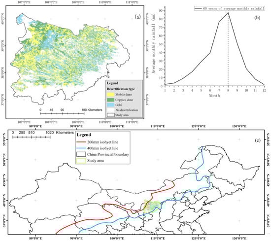
Figure 1.
(a) Desertification types in the study area; (b) annual mean monthly precipitation in the study area; (c) location of the study area in a semi-arid region of China.
The annual total precipitation in the Mu Us Sandy Land region decreases from southeast to west, ranging from 440 mm to 250 mm [6]. As shown in Figure 1b, the peak monthly precipitation occurs in August. The annual average precipitation is about 340 mm, which is higher than that of other sandy lands. From 1995 to 2019, the precipitation in 1999–2000 was significantly lower than the average precipitation of the past 60 years. The precipitation in 2005 was also very low, but in 2004 it was slightly above the long-term average. The annual average precipitation in 2010 and 2011 was basically the same as that of many years, while the annual average precipitation in 2014 and 2015 was slightly below the long-term average for two consecutive years. The Mu Us Sandy Land region has an annual average temperature ranging from 6 °C to 8.5 °C, and the temperature decreases from south to north. The region also belongs to the arid to semi-arid climate region, with a maximum wind speed of up to 28 m/s [44].
2.2. NPV and PV Data Sources and Calculation Methods
This study utilized MODIS NDVI 8-day products and SWIR76 data to calculate the monthly average NPV, PV, and bare soil products from 2000 to 2015, based on linear spectral unmixing. This approach was developed by Guerschman et al. [5] using hyperspectral data collected from over 1000 field sites. The SWIR76 index is defined as the ratio of the SWIR7 band (2130 nm) to the SWIR6 band (1640 nm) in MODIS data.
It is important to note that the spatial resolution of MODIS data, which is greater than 250 m, may result in inaccurate analysis of NPV and PV in the Mu Us desert area, where shrub desertification is predominant. Consequently, a key focus of this study is to develop NPV and PV estimation models using Landsat series imagery through machine learning techniques.
The construction process of the machine learning model in this study is divided into three parts: data collection for the model output, external validation of the model, and model selection. First, data collection for the model output used UAV imagery collected in the field, covering a total of 457 points from 2017 to 2023. The UAV imagery processing included radiometric correction and mosaicking, object-based multiscale segmentation, resulting in NPV, PV, and bare soil cover data for 457 points, each with a spatial coverage exceeding 30 × 30 m. Second, the input for model construction consisted of Landsat spectral data corresponding to the UAV sampling points. With both the output and input data combined to form the dataset, 70% of the data were used to build the model, and 30% were used for the test set. To minimize the impact of data distribution bias on accuracy, ten-fold cross-validation was employed to average the final accuracy. Notably, the data used for model construction were also split into a training set and a validation set at a 70% to 30% ratio. Finally, the model selection was based on the final accuracy obtained from the ten-fold cross-validation of the test set.
The formulas mentioned in the above methods are explained as follows. In Formulas (1) and (2), is the predicted value, is the true value, is the average of the predicted values, and n is the number of samples.
The ten-fold cross-validation method is commonly used to test the accuracy of algorithms. It involves dividing the dataset into 10 parts, then iteratively using 9 parts as training data and 1 part as test data. Each iteration yields an accuracy (or error) rate, and the average of the ten results provides an estimate of the algorithm’s precision.
The development of a machine learning model first requires the identification of its inputs and outputs. The model inputs will include indices such as NDVI (Normalized Difference Vegetation Index) [18], Enhanced Vegetation Index (EVI) [19], Normalized Difference Senescence Vegetation Index (NDSVI) [20], Landsat 8-OLI Dead Fuel Index (OLI-DFI) [21], Modified Soil-Adjusted Vegetation Index (MSAVI) [22], Ci-green, and Normalized Difference Index (NDI) [23].
In this study, the mesh search method is used in the parameter adjustment process of the machine learning model. The parameter settings for the model tested in this study are detailed as follows:
RF Parameters: To optimize for minimal mean squared error (MSE) and fast convergence, the parameters for the RF regression models, specifically for NPV and PV, were set with a minimum of five leaf nodes and requiring over 50 decision trees. Additional parameters, such as the depth of individual trees and the number of features considered by each tree, were fine-tuned based on MSE values during the algorithmic process.
BP Neural Network Parameters: The BP neural network comprises three layers. The transfer function from the input layer to the first hidden layer is the logsig function, with the number of neurons experimentally determined. From the first hidden layer to the second hidden layer, the transfer function is the softmax function, ensuring the sum of the three neurons in the output layer equals one. The transition from the second hidden layer to the output layer utilizes the purelin function. The output layer consists of three nodes representing the fractions of NPV, PV cover, and bare soil within a pixel. The error loss function employed is the mean squared error function, and the gradient descent is executed using the Levenberg–Marquardt algorithm. To ensure model convergence, the learning rate and maximum number of fail attempts were set to 0.01 and 10, respectively.
FCNN Parameters: Apart from the input and output layers, this deep learning network includes five hidden layers, each with 128 neurons and the rectified linear unit (ReLU) function as the transfer function between layers. The overall performance of each model is illustrated in Appendix A Figure A1.
The preprocessing of the remote sensing images included radiometric correction, geometric correction, color balancing, and mosaicking. Atmospheric correction was performed using the FLAASH module in ENVI. Histogram matching was conducted for other images and test period images, followed by mosaicking of all employed images. This study downloaded all low-cloud-cover Landsat 5 TM images taken from 17 September to 17 October for the years 2000 to 2012. Considering the dates and cloud cover, the missing images were replaced with those from the same period in the previous or following year. For the data from 2013 to 2019, Landsat 8-OLI images from 17 September to 17 October were used. Similarly, missing images were substituted with those from the same period in the previous or following year, considering both dates and cloud cover. The frequency of image acquisition for each period and the corresponding sensors are documented in Appendix A Table A1, Table A2, Table A3 and Table A4.
The Landsat Operational Land Imager (OLI) and Thematic Mapper (TM) sensors have been found to show differences in reflection values for the same ground objects. For instance, in urban mapping, the reflectance difference of Landsat 8-OLI images for different ground objects is more noticeable than that of Landsat 5 TM [45]. However, some studies have shown that there is a high correlation between vegetation indices and reflectance of the same ground object using different sensors in large and uniform areas [46]. To account for these differences, a regression relationship between the Landsat 8-OLI and Landsat 5 TM bands was established before building the NPV and PV coverage detection models for Landsat 5 TM images. The reflection values of Landsat 8-OLI images corresponding to sample points were then back-calculated to reflect the values of Landsat 5 TM images through this regression relationship. Finally, a new machine learning regression fitting model was built using the NPV coverage and PV coverage data from UAV sampling points.
2.3. Precipitation and SPEI Data
The quadratic thin plate spline function is a type of interpolation method commonly used to interpolate meteorological data. In this study, it was used to interpolate precipitation and temperature data at 500 m and 30 m resolutions. Elevation was also used as a covariate in the interpolation process. The data used for interpolation were based on measurements from 19 meteorological stations located in the Mu Us Sandy Land and its surrounding areas. The interpolation was carried out for both annual and monthly total precipitation and annual mean temperature.
The Standardized Precipitation-Evapotranspiration Index (SPEI), proposed by Vicente-Serrano et al. [47] as an extension of the Standardized Precipitation Index (SPI), represents the dry and wet conditions of a region based on the degree of deviation between precipitation and potential evapotranspiration from the average state. In this study, the Penman–Monteith formula was preferred for calculating potential evapotranspiration in arid and semi-arid regions. Four-time scales of SPEI were calculated, including SPEI-1 for 1-month conditions, SPEI-3 for 3-month conditions, SPEI-6 for 6-month conditions, and SPEI-12 for 12-month conditions. Table 1 shows the classification of dry and wet conditions.

Table 1.
Classification of drought and wet grade based on SPEI.
2.4. Temporal and Spatial Regression Analysis
In this study, the PV and NPV from September 2001 to September 2019 were analyzed using pixel-by-pixel regression with MODIS NPV and PV products having a resolution of 500 m. The annual total precipitation and annual mean temperature of the same resolution were used for the analysis. The time delay effect of the current year refers to the total precipitation and average temperature from January to September of the image year, while the time delay effect of the previous year refers to the total precipitation and average temperature from 10–21 months before the image acquisition month. Similarly, the time delay effects for the first two years (22–33 months), the first three years (34–45 months), and the first four years (46–57 months) were also analyzed.
Regression analysis was conducted at a regional scale to explain the response of NPV and PV coverage, calculated from Landsat series images, to precipitation and multi-scale SPEI. The monthly total rainfall data for the first 21 months of the NPV and PV coverage data of the current period were considered. For example, when the data for the period were from Landsat image with the strip number 127032 in 2005 (obtained on 7 October), the corresponding rainfall data were from January 2004 to September 2005. Similarly, the NPV and PV data were analyzed against the cumulative drought and moisture conditions on four-time scales of SPEI-1, SPEI-3, SPEI-6, and SPEI-12 using SPEI data. In this study, these datasets were used to analyze the response of spatial patterns of vegetation to precipitation in the geographical ecological region.
Based on the explanation of the above methods and data, the technical flowchart of this research is shown in Figure 2.
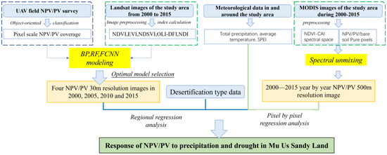
Figure 2.
Technical workflow diagram of this study.
3. Results
3.1. Machine Learning Model Construction for Estimating NPV/PV Cover
This study assessed the performance of random forest (RF), backpropagation (BP), and fully connected neural network (FCNN) models in the remote sensing retrieval of NPV and PV. The accuracy results from ten-fold cross-validation are presented in Table 2. It is evident that the RF algorithm excelled in model generalization performance, whereas both BP and FCNN models exhibited subpar generalization performance, especially the FCNN, with the cross-validated (R2 and RMSE) for the NPV model even falling below 0.53.
Table 2.
Accuracy table for estimating NPV and PV by different machine learning models.
This study concludes that when applying a backpropagation-type FCNN, using the logsig function as the transfer function is preferable. It was observed that when all linking functions are ReLU, simply increasing the number of layers and neurons does not significantly enhance the model’s generalization ability. In a separate study conducted by our team, we investigated the generalization capabilities of ensemble algorithms and backpropagation neural networks for detecting NPV. Based on the comprehensive results from these studies, we conclude that the random forest model is more advantageous for the remote sensing inversion of NPV and PV in arid and semi-arid ecosystems.
Subsequently, this study validated the MODIS NPV and PV products derived through the spectral unmixing method. The RMSE for PV was 25%, and for NPV, it was 33%. We consider this product’s trend across the entire study area to be reliable, enabling its utilization in analyzing the impacts of annual total precipitation and mean temperature on NPV and PV. When testing the inversion of MODIS NPV and PV using RF, BPNN, and FCNN models, the R2 values were all below 0.2. This indicates that the machine learning models developed using Landsat imagery cannot be applied to MODIS data.
3.2. Inversion Results and Statistical Characteristics of NPV and PV across Different Periods
Upon determining the use of the RF algorithm for the inversion of NPV and PV in the study area, this research selected Landsat images from four periods: 2000, 2005, 2010, and 2015. To ensure consistency between Landsat 5 and Landsat 8 images, areas with unchanged features such as buildings, forests, and deserts were used to perform regression correction on the band values. The correction relationships are illustrated in Appendix A Figure A2.
The NPV and PV retrieved by the RF model for the years 2000, 2005, 2010, and 2015 are presented in Appendix A Figure A3, Figure A4, Figure A5 and Figure A6, with box plot statistics segmented by different types of desertification displayed in Figure 3 and Figure 4 of the main text. The images from top to bottom represent light, moderate, and severe desertification, while the images from left to right represent different types of desertification. The red symbols in the figures represent outliers that exceed the overall distribution by a factor of 1.5 quartiles.
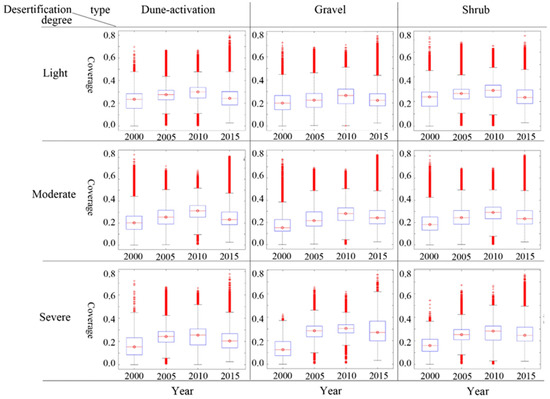
Figure 3.
Box plot of non-photosynthetic vegetation coverage of different desertification types and degrees.
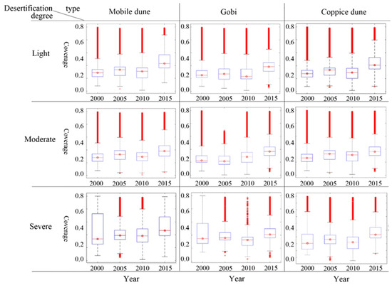
Figure 4.
Box plot of photosynthetic vegetation coverage of different desertification types and degrees.
The coverage of NPV in coppice dunes was found to be higher than in the desertification region. Additionally, it was observed that the higher the degree of desertification, the lower the NPV coverage. The coverage of NPV showed significant variation across different years, suggesting that it is influenced by climatic factors.
The coverage of PV (as shown in Figure 4) also exhibited significant fluctuations in different years. Furthermore, as depicted in Figure A5b in Appendix A, PV was exceptionally high in 2015. These observations highlight the sensitivity of NPV and PV to climate, and we aim to further explore the extent of climate influence in the subsequent sections.
3.3. NPV and PV Response to Annual Precipitation and Temperature
The NPV and PV data for the end of the growing season from 2001 to 2019 were obtained by calculating MODIS data. The accuracy of the linear spectral unmixing results was verified by comparing them with the real values of the field sampling points. In this study area, the RMSE for PV was 25% and for NPV was 33%. The effects of average temperature and total precipitation on NPV and PV at the end of the growing season were analyzed, and the results are shown in Figure 5 and Figure A7, Figure A8, Figure A9 and Figure A10 in Appendix A.
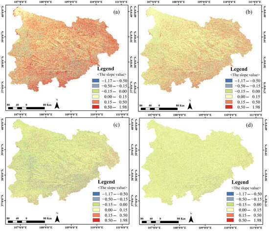
Figure 5.
(a) Response of non-photosynthetic vegetation to annual precipitation. (b) Response of photosynthetic vegetation to annual precipitation. (c) Response of non-photosynthetic vegetation to annual mean temperature. (d) Response of photosynthetic vegetation to annual mean temperature.
It was found that, when considering the effect of precipitation on vegetation at an annual time scale, NPV is more responsive than PV to precipitation. Precipitation has a positive effect on vegetation, while temperature has a weak negative effect (with a slope of less than 0.15 in most areas). The effects of temperature and precipitation varied significantly across different land cover types. In particular, in sandy land areas, the impact of temperature and precipitation on NPV and PV over a long-term time scale was found to be minimal. In contrast, grassland and shrub areas exhibited a certain degree of response to long-term precipitation and temperature.
Based on Figure A7 in Appendix A, the maximum impact of total precipitation on NPV occurred between 33 and 45 months. Meanwhile, the response of PV to total precipitation from January to September was more evident (Figure A8 in Appendix A). The effect of average temperature on NPV varied slightly with different time delay scales. In a typical steppe area, the coverage of NPV tended to decrease as temperature increased, but the overall influence was relatively low across the study area (Figure A9 in Appendix A). PV, on the other hand, had a very low response to average temperature at different time delay scales, indicating that air temperature may not be the primary factor influencing changes in PV coverage (Figure A10 in Appendix A).
3.4. Effects of Monthly Time Scale Precipitation on NPV and PV Spatial Distribution
Four periods of NPV and PV data from 2000, 2005, 2010, and 2015 (as shown in Figure A3, Figure A4, Figure A5 and Figure A6 in Appendix A) were analyzed for regional correlation with meteorological data. The results of the analysis are shown in Figure 6 and Figure 7. Among them, the years 2010 (wet year) and 2000 (dry year) are representative. For ease of understanding, we will only include figures for the years 2000 and 2015 in the main text. The impact of monthly precipitation on NPV and PV in the years 2005 and 2010 can be found in Appendix A Figure A11 and Figure A12. Each column in the figures represents a different desertification type, while each row represents a different year.
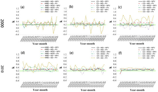
Figure 6.
(a) Time-Lagged Response of NPV and PV to Monthly Precipitation on mobile dune desertification during Dry Years. (b) Time-Lagged Response of NPV and PV to Monthly Precipitation on coppice dune desertification during Dry Years. (c) Time-Lagged Response of NPV and PV to Monthly Precipitation on Gobi desertification during Dry Years. (d) Time-Lagged Response of NPV and PV to Monthly Precipitation on mobile dune desertification during Wet Years. (e) Time-Lagged Response of NPV and PV to Monthly Precipitation on coppice dune desertification Wet Years. (f) Time-Lagged Response of NPV and PV to Monthly Precipitation on Gobi desertification Wet Years. Figure note: MBD represents mobile dune desertification; CD represents coppice dune desertification; GD represents Gobi desertification; MD represents mild desertification; MOD represents moderate desertification; and SD represents severe desertification. K is the response degree of NPV and PV to precipitation in the desertification type and degree region.
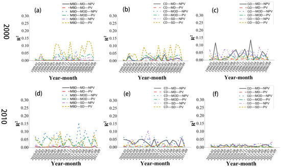
Figure 7.
(a) Time-delay correlation (R2) of NPV and PV to Monthly Precipitation on mobile dune desertification during Dry Years. (b) Time-delay correlation (R2) of NPV and PV to Monthly Precipitation on coppice dune desertification during Dry Years. (c) Time-delay correlation (R2) of NPV and PV to Monthly Precipitation on Gobi desertification during Dry Years. (d) Time-delay correlation (R2) of NPV and PV to Monthly Precipitation on mobile dune desertification during Wet Years. (e) Time-delay correlation (R2) of NPV and PV to Monthly Precipitation on coppice dune desertification Wet Years. (f) Time-delay correlation (R2) of NPV and PV to Monthly Precipitation on Gobi desertifi-cation Wet Years. Figure note: MBD represents mobile dune desertification; CD represents coppice dune desertification; GD represents Gobi desertification; MD represents mild desertification; MOD represents moderate desertification; and SD represents severe desertification. R2 is the correlation.
Figure 6 illustrates that in the regional regression relationship established between monthly precipitation and NPV/PV, most of the slopes exceed 0.25 (the position of the green horizontal boxes in the figure is generally around 0.25). This indicates that for every 1 mm increase in precipitation in the study area, NPV and PV may increase by approximately 0.25%. The response of NPV and PV to precipitation varied significantly for different desertification types and degrees within the first 21 months. In Figure 7, the R2 values indicate weak correlations in a statistical sense. However, based on the principle of regional relevance, if a particular rainfall event leads to an overall increase in NPV/PV for a specific desertification type and exhibits higher correlation compared to other rainfall events, it suggests that this rainfall event has a certain degree of influence on NPV/PV.
The PV coverage at the end of the growing season in areas of moderate and severe desertification showed correlation with precipitation in winter, the preceding, and current growing seasons. Specifically, the PV coverage of moderate and severe mobile dunes and coppice dunes showed more distinct changes to precipitation in different months (yellow dotted line and green dotted line in Figure 6 and Figure 7). The PV coverage of moderate and severe desertification in the Gobi type (Figure 6c) fluctuated more in response to monthly precipitation in arid years (2000, 2005, and 2015) than in other types and degrees of desertification. However, the fluctuation decreased in the years with a humid climate (2010) (Figure 6f).
NPV (black line in Figure 7) and PV (red dashed line) of mild desertification exhibit a relatively stable response to rainfall and do not fluctuate significantly with the occurrence of rainfall events. In the desertification types of Gobi and sand dune reactivation, mildly desertified NPV shows a higher correlation with rainfall events (Figure 7c). PV and NPV information on moderate and severe desertification is more sensitive to precipitation changes, and this sensitivity becomes more pronounced with the increasing severity of drought (Figure 7). The dependence of PV and NPV on precipitation in coppice dune desertification and mobile dune desertification was greater in arid years than in long-term humid years (Figure 7b,e).
Overall, the response of NPV and PV to rainfall events is complex and influenced by factors such as vegetation type, duration of drought, rainfall frequency, and other related factors. Therefore, in the following section, we attempt to further elucidate certain issues by combining the duration of drought with the occurrence of rainfall events.
3.5. Effects of Drought on NPV and PV Spatial Distribution at Different Time Scales
3.5.1. Occurrence of Drought in the Study Area
In this section, we will measure the impact of drought on the spatial distribution of NPV and PV using the SPEI index. The measurements will be taken at scales of 1, 3, 6, and 12 months. The SPEI at different time scales at the end of the growing season is shown in Figure A13, Figure A14, Figure A15 and Figure A16 in Appendix A. The end of the growing season in 2000 had a prolonged and severe drought from July to September, with the SPEI values consistently below −2.0. In 2005, the typical grassland area experienced a continuous drought, although the overall drought severity was lower than that of 2000. In 2010, the area was continuously wet, while 2015 was characterized by a prolonged moderate drought. During the growing season, the drought severity ranged from moderate to severe, but at the end of the growing season, there were extreme wet conditions.
3.5.2. Impact of Drought and Rainfall Events on NPV and PV
The average effects of SPEI on NPV and PV were approximately 0.3, and these effects varied depending on the year and type of desertification, as shown in Figure 8 and Figure 9. Specifically, the PV coverage of severe desertification showed a stronger response to SPEI. In the persistent drought year of 2000, the PV coverage had a stronger response to drought events at the 12-month scale (the orange line in Figure 8a–c), while in the persistent wet year of 2010, the PV coverage had a stronger response to wet events at the 1-month and 3-month scales (the orange line in Figure 8g–i). The response of PV coverage to SPEI increased after extreme humid events occurred following long-term drought in 2015 (the orange line in Figure 8j–l). The response of PV coverage to SPEI over three months was still higher for PV with severe desertification.
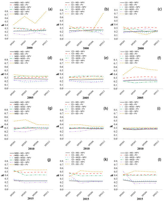
Figure 8.
(a) Response of NPV and PV to SPEI on mobile dune desertification in the Year 2000. (b) Response of NPV and PV to SPEI on coppice dune desertification in the Year 2000. (c) Response of NPV and PV to SPEI on Gobi desertification in the Year 2000. (d) Response of NPV and PV to SPEI on mobile dune desertification in the Year 2005. (e) Response of NPV and PV to SPEI on coppice dune desertification in the Year 2005. (f) Response of NPV and PV to SPEI on Gobi desertification in the Year 2005. (g) Response of NPV and PV to SPEI on mobile dune desertification in the Year 2010. (h) Response of NPV and PV to SPEI on coppice dune desertification in the Year 2010. (i) Response of NPV and PV to SPEI on Gobi desertification in the Year 2010. (j) Response of NPV and PV to SPEI on mobile dune desertification in the Year 2015. (k) Response of NPV and PV to SPEI on coppice dune desertification in the Year 2015. (l) Response of NPV and PV to SPEI on Gobi desertification in the Year 2015. Figure note: MBD represents mobile dune desertification; CD represents coppice dune desertification; GD represents Gobi desertification; MD represents mild desertification; MOD represents moderate desertification; and SD represents severe desertification. K is the response degree of NPV and PV to precipitation in the desertification type and degree region.
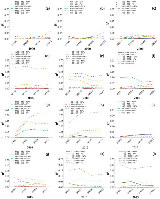
Figure 9.
(a) Correlation of NPV and PV to SPEI on mobile dune desertification in the Year 2000. (b) Correlation of NPV and PV to SPEI on coppice dune desertification in the Year 2000. (c) Correlation of NPV and PV to SPEI on Gobi desertification in the Year 2000. (d) Correlation of NPV and PV to SPEI on mobile dune desertification in the Year 2005. (e) Correlation of NPV and PV to SPEI on coppice dune desertification in the Year 2005. (f) Correlation of NPV and PV to SPEI on Gobi desertification in the Year 2005. (g) Correlation of NPV and PV to SPEI on mobile dune desertification in the Year 2010. (h) Correlation of NPV and PV to SPEI on coppice dune desertification in the Year 2010. (i) Correlation of NPV and PV to SPEI on Gobi desertification in the Year 2010. (j) Correlation of NPV and PV to SPEI on mobile dune desertification in the Year 2015. (k) Response of NPV and PV to SPEI on coppice dune desertification in the Year 2015. (l) Response of NPV and PV to SPEI on Gobi desertification in the Year 2015. Figure note: MBD represents mobile dune desertification; CD represents coppice dune desertification; GD represents Gobi desertification; MD represents mild desertification; MOD represents moderate desertification; and SD represents severe desertification. R2 is the correlation.
In contrast, the response of NPV to SPEI was lower than that of PV, particularly for the severe desertification type where NPV had the lowest response. The response of NPV to SPEI at different time scales showed little change, but the response of NPV to SPEI at 6 and 12 months was slightly higher, with an average effect of approximately 0.2. In 2015, the NPV of severely desertified land showed a significantly higher response to extreme humid events, with an effect size of approximately 0.5 (the black, blue, and purple lines in Figure 8j–l).
Overall, the correlation between SPEI and NPV and PV varies depending on the year and type of desertification. In 2000, when drought was severe and continuous, the correlation between SPEI and NPV/PV spatial distribution was weak due to the extremely dry growing seasons (Figure 9a–c). In 2005, mild to moderate drought resulted in a higher correlation between SPEI and NPV/PV for moderate desertification (Figure 9d–f). In 2010, severe mobile dune and coppice dune desertification had a strong correlation with long-term humidity events (Figure 9g–i). In 2015, severe desertification NPV had a good correlation with SPEI, especially for Gobi and coppice dune desertification, which had a strong correlation with extreme humid events (Figure 9j–l).
The SPEI has a stronger ability to explain the spatial distribution of NPV and PV than precipitation. Due to the occurrence of drought and humid events in different years, the SPEI has a greater effect on the spatial distribution of NPV and PV. Long-term drought had a significant influence on the photosynthetic information of severe desertification, while short-term moisture had a great influence on the photosynthetic information, and long-term moisture had a high correlation with the spatial distribution of non-photosynthetic information.
4. Discussion
4.1. Uncertainty and Error Sources in the NPV and PV Products of This Study
As shown in Appendix A Figure A1, 85% of the errors in the final RF model adopted in this study fall within the range of 0.1113. Here, we attempt to discuss the uncertainty in NPV and PV products and the potential sources of error.
4.1.1. Nonlinear Mixing Effects of NPV, PV, and Bare Land at 500 m Scale
The time series linear regression analysis of NPV, PV coverage, and precipitation from MODIS data revealed a discernible trend, but with a significant gap between adjacent pixels. For the MODIS43 data product used by Guerschman et al. [16], the effect of such noise points was significant after smooth filtering, and they should not still be present in the results of this study. However, as shown in Figure 10, there are still some noise points (blank pixels in Figure 10a,c) with different positions in MODIS NPV and PV coverage for two consecutive years.
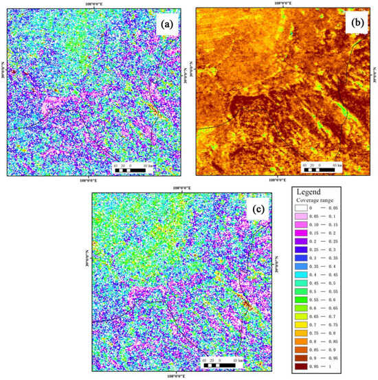
Figure 10.
(a) Local NPV cover of MODIS in 2019; (b) SWIR67 Index in 2019; (c) Local NPV of MODIS in 2018.
In other similar studies in semi-arid regions of China, the end element value was considered, and the calculated results still demonstrated this phenomenon. Therefore, in arid and semi-arid regions, the 500 m pixel scale mixes a lot of ground objects, leading to a nonlinear mixing effect. Considering the presence of such nonlinear mixing effects, this study also employed machine learning models on MODIS imagery. However, due to the mixed effects of different shrubs at the 500 m scale, the spectral differences between pixels with the same NPV and PV cover were excessively large. As a result, the machine learning models for MODIS NPV and PV based on the original dataset exhibited poor accuracy, with R2 values not exceeding 0.2.
4.1.2. Potential Effects of Soil Properties and Vegetation Types on NPV Machine Learning Models
Soil, sediments, and minerals in rocks exhibit strong absorption characteristics in the SWIR2 spectral region [48], complicating the estimation of NPV coverage using lignocellulose absorption. Specifically, methods that characterize NPV using only a single SWIR2 band (e.g., NDTI) are more susceptible to variations in surface cover, surface moisture, and soil properties. In our study area, the predominant soil type is sandy soil. Measurements of bare soil, NPV, and PV using a spectrometer within the 400–900 nm range indicate that sandy soil impacts PV detection from 760 to 900 nm, but distinctions remain clear within the 400–760 nm range, as illustrated in Figure 11.

Figure 11.
Spectra of photosynthetic and non-photosynthetic components of major vegetation types and major soil types in the study area.
Additionally, water within plant tissues can alter or obscure the lignocellulose absorption features at 2100 nm [49]. Figure 11 also displays variances in the spectral characteristics of different plants’ NPV in our study area, though the distinction between NPV and PV remains consistent when using different band combinations.
Multiple researchers have highlighted that using multiple SWIR2 bands rather than a single SWIR2 band improves the performance of NPV characterization [50,51,52]. Consequently, employing multiple band combinations can mitigate the influence of soil type and vegetation type on machine learning models predicting NPV and PV. However, if the study scope expands, the machine learning models developed in this research will need to reintegrate vegetation and soil types, thereby increasing the sample diversity.
4.2. Long Time Delay Effect of Precipitation on NPV
Numerous studies have demonstrated that increased precipitation significantly enhances litter production and decomposition, while warming can accelerate litter decomposition rates [42,53,54]. These findings are consistent with the responses of NPV to precipitation and temperature observed in this study. Additionally, another study in the arid and semi-arid regions of northern China indicated that litter quality is more likely affected by the interval between precipitation events rather than the reduction in precipitation itself. Drought has been identified as the primary factor influencing litter quality [8].
Our study analyzed the effects of rainfall and drought on NPV and PV and similarly found that when rainfall continued to decrease and meteorological drought continued to accumulate, the responses of NPV to rainfall became more pronounced. In years with prolonged drought, NPV is correlated with precipitation during the late winter and growing season, which is consistent with the findings of Liang [55]. This implies that in drought years, vegetation communities rely more heavily on groundwater recharge during the winter. This underscores the importance of focusing on the time-lag and cumulative effects of meteorological events such as droughts in future research on arid and semi-arid ecosystems.
Simultaneously, considering the type and degree of desertification can help us understand that litter is more susceptible to drought and cumulative drought in ecologically vulnerable areas with severe desertification. Litter can help retain water, reduce soil temperature, and reflect the resilience of vegetation communities to climate disturbances. Therefore, including NPV as a remote sensing indicator of the stability of arid and semi-arid ecological communities in subsequent studies holds great scientific significance.
4.3. Response of PV to Short-Term Precipitation
The study by Tang et al. [56] showed that the response of carbon flux to precipitation in arid and semi-arid ecosystems is related to the amount and timing of rainfall and early soil moisture. Similarly, the study by Xu et al. [33] demonstrated that the duration of drought affects the response of ecosystem photosynthesis. Consistent with these findings, this present study found that under the cumulative effect of long-term drought, extreme humid events led to a significant increase in PV coverage. A study on the response of the photosynthetic characteristics of plant communities in similar ecological environments to drought concluded that the ecosystem had strong resistance to soil drought and high temperature, maintained long-time light-use efficiency during drought, and increased photosynthetic capacity rapidly when the soil was wet [57]. According to Nakano, Nemoto, and Shinoda [34], ecosystem respiration surged after a heavy rainfall event. The short-term response of PV to rainfall and drought reflects the resilience of arid and semi-arid ecosystems after extreme climate events.
4.4. Research Shortcomings and Prospects
In the analysis conducted in this study, we did not examine the nonlinear effects of climate on vegetation, nor did we consider the short-term cumulative effects of precipitation on plant communities. Instead, we focused solely on the lag effects. Future research should integrate multiple factors, such as surface temperature, human activities, and soil moisture, employing nonlinear analytical models to investigate the causes of dynamic changes in ecosystems in arid and semi-arid regions.
Our study posits that NPV and PV are robust indicators of the health status and resilience of arid and semi-arid ecosystems to extreme climate events. This implies that in arid and semi-arid ecosystems, the mutual feedback effects between PV, NPV, and water will provide new insights and perspectives for the study of vegetation pattern dynamics. Additionally, it will offer crucial evidence for researching the resistance and sensitivity of these ecosystems to climate change. Furthermore, since NPV encompasses both litter and standing dead biomass, investigating the relationships among PV, NPV, and soil organic carbon will also provide important methods for spatial quantification of the carbon cycle in arid and semi-arid ecosystems.
5. Conclusions
The main conclusions of this study are as follows:
- Spectral Variability and Machine Learning Models: In arid and semi-arid regions, the mixture of shrubs and herbaceous plants leads to significant spectral variability at different spatial scales for the same location. Consequently, machine learning models developed for NPV and PV using Landsat imagery cannot be directly transferred to MODIS imagery. Neural networks that only use the RELU activation function, even in deep learning models, perform poorly in NPV inversion tasks. In contrast, random forests, as an ensemble method, demonstrate superior inversion accuracy for both NPV and PV.
- PV, NPV, and Monthly Precipitation: The response of PV to monthly precipitation was greater than that of NPV, with a more obvious response observed in areas with higher degrees of desertification.
- PV, NPV, and Drought Accumulation: The accumulation time of drought significantly influenced NPV and the response of PV to climate. In areas with more severe desertification, the response of NPV to cumulative drought was more pronounced. Under conditions of cumulative drought, both NPV and PV were highly dependent on precipitation during the growing season and winter of the previous year. However, their dependence on precipitation decreased under cumulative wetting conditions.
- PV and Extreme Humid Events: After a long-term drought, extreme humid events can lead to an increase in the coverage of moderate and mild desertification PV, whereas the response of severe desertification PV to extreme humid events is less pronounced than its response to long-term drought.
Author Contributions
Conceptualization, S.L. and Z.G.; methodology, Z.G.; validation, Z.G.; formal analysis, Z.G.; investigation, S.L., Z.G., W.K., X.C. and K.F.; writing—original draft preparation, Z.G.; writing—review and editing, Z.G. All authors have read and agreed to the published version of the manuscript.
Funding
This study is supported by the National Natural Science Foundation of China (Grant No. 42307564), National Natural Science Foundation of China (Grant No. 42271316), and Science and Technology Department of Gansu Province, Key R&D Program (Grant No. 21YF5NA070).
Data Availability Statement
Restrictions apply to the datasets. The datasets presented in this article are not readily available because the data are part of an ongoing study.
Acknowledgments
Thanks to the responsible editors and reviewers for their work and effective suggestions.
Conflicts of Interest
The authors declare no conflicts of interest.
Appendix A
Table A1.
Images used in 2000–2001 and their acquisition schedule.
Table A1.
Images used in 2000–2001 and their acquisition schedule.
| Landsat 5 Ranks No. | Image Acquisition Time | Reference (R) or Adjust (A) | Landsat 5 Ranks No. | Image Acquisition Time | Reference or Adjust |
|---|---|---|---|---|---|
| 128033 | 20000917 | R | 127034 | 20000926 | A |
| 128034 | 20000917 | A | 129033 | 20011017 | A |
| 127032 | 20000926 | A | 129034 | 20000924 | A |
| 127033 | 20000926 | A |
Table A2.
Images used in 2004–2005 and their acquisition schedule.
Table A2.
Images used in 2004–2005 and their acquisition schedule.
| Landsat 5 Ranks No. | Image Acquisition Time | Reference (R) or Adjust (A) | Landsat 5 Ranks No. | Image Acquisition Time | Reference or Adjust |
|---|---|---|---|---|---|
| 128033 | 20040928 | R | 127034 | 20040922 | A |
| 128034 | 20040928 | A | 129033 | 20050922 | A |
| 127032 | 20051007 | A | 129034 | 20051007 | A |
| 127033 | 20040922 | A |
Table A3.
Images used in 2010–2011 and their acquisition schedule.
Table A3.
Images used in 2010–2011 and their acquisition schedule.
| Landsat 5 Ranks No. | Image Acquisition Time | Reference (R) or Adjust (A) | Landsat 5 Ranks No. | Image Acquisition Time | Reference or Adjust |
|---|---|---|---|---|---|
| 128033 | 20100912 | R | 127034 | 20101007 | A |
| 128034 | 20100912 | A | 129033 | 20110922 | A |
| 127032 | 20101007 | A | 129034 | 20110922 | A |
| 127033 | 20101007 | A |
Table A4.
Images used in 2014–2015 and their acquisition schedule.
Table A4.
Images used in 2014–2015 and their acquisition schedule.
| Landsat 5 Ranks No. | Image Acquisition Time | Reference (R) or Adjust (A) | Landsat 5 Ranks No. | Image Acquisition Time | Reference or Adjust |
|---|---|---|---|---|---|
| 128033 | 20141007 | R | 127034 | 20151005 | A |
| 128034 | 20141007 | A | 129033 | 20150917 | A |
| 127032 | 20151005 | A | 129034 | 20150917 | A |
| 127033 | 20151005 | A |

Figure A1.
(a) Process of parameter selection for RF models. (b) Error distribution of random forest models. (c) Process of parameter selection for BPNN. (d) Process of parameter selection for FCNN.
Figure A1.
(a) Process of parameter selection for RF models. (b) Error distribution of random forest models. (c) Process of parameter selection for BPNN. (d) Process of parameter selection for FCNN.
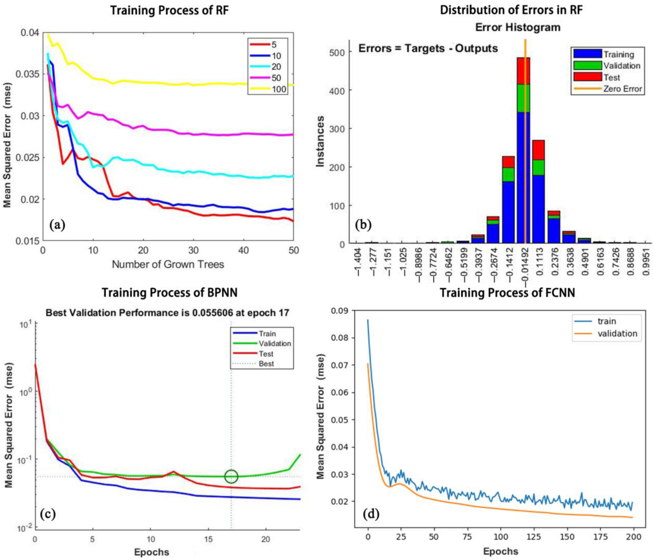

Figure A2.
(a) The regression relationship between Landsat 8 B2 and Landsat 5 B1. (b) The regression relationship between Landsat 8 B3 and Landsat 5 B2. (c) The regression relationship between Landsat 8 B4 and Landsat 5 B3. (d) The regression relationship between Landsat 8 B5 and Landsat 5 B4. (e) The regression relationship between Landsat 8 B6 and Landsat 5 B5. (f) The regression relationship between Landsat 8 B7 and Landsat 5 B6.
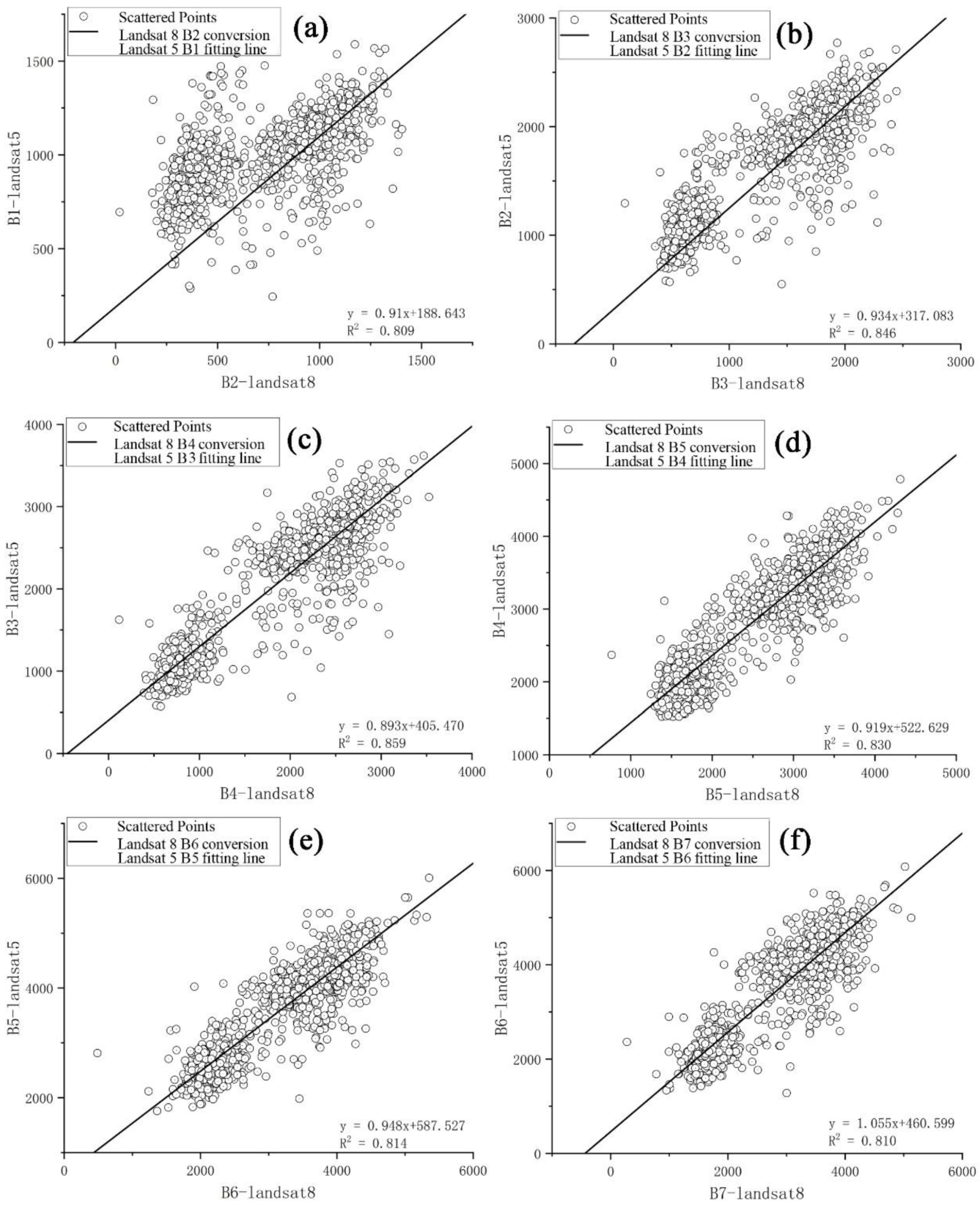
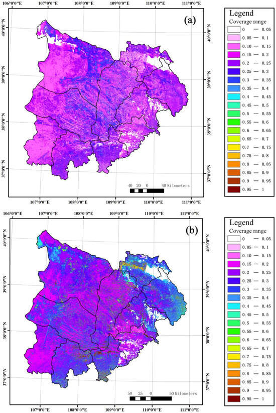
Figure A3.
(a) Non-photosynthetic vegetation coverage at the end of the growing season in 2000. (b) Photosynthetic vegetation coverage at the end of the growing season in 2000.
Figure A3.
(a) Non-photosynthetic vegetation coverage at the end of the growing season in 2000. (b) Photosynthetic vegetation coverage at the end of the growing season in 2000.

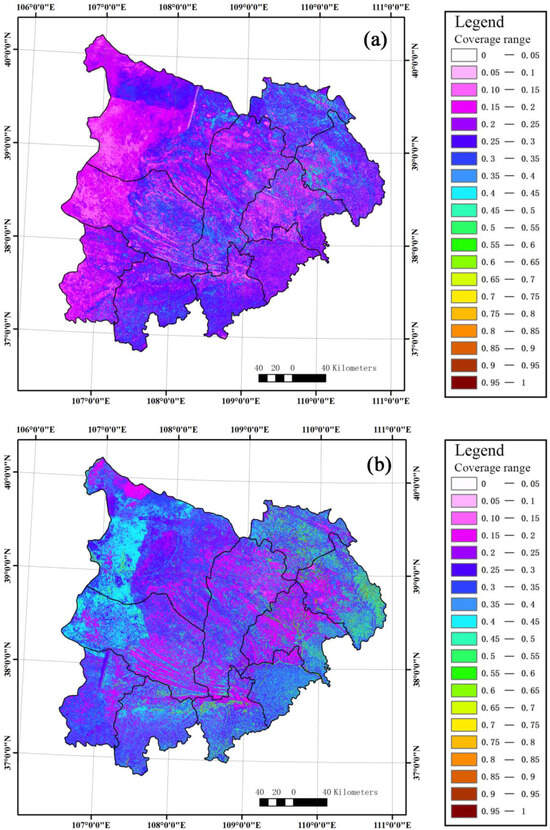
Figure A4.
(a) Non-photosynthetic vegetation coverage at the end of the growing season in 2005. (b) Photosynthetic vegetation coverage at the end of the growing season in 2005.
Figure A4.
(a) Non-photosynthetic vegetation coverage at the end of the growing season in 2005. (b) Photosynthetic vegetation coverage at the end of the growing season in 2005.
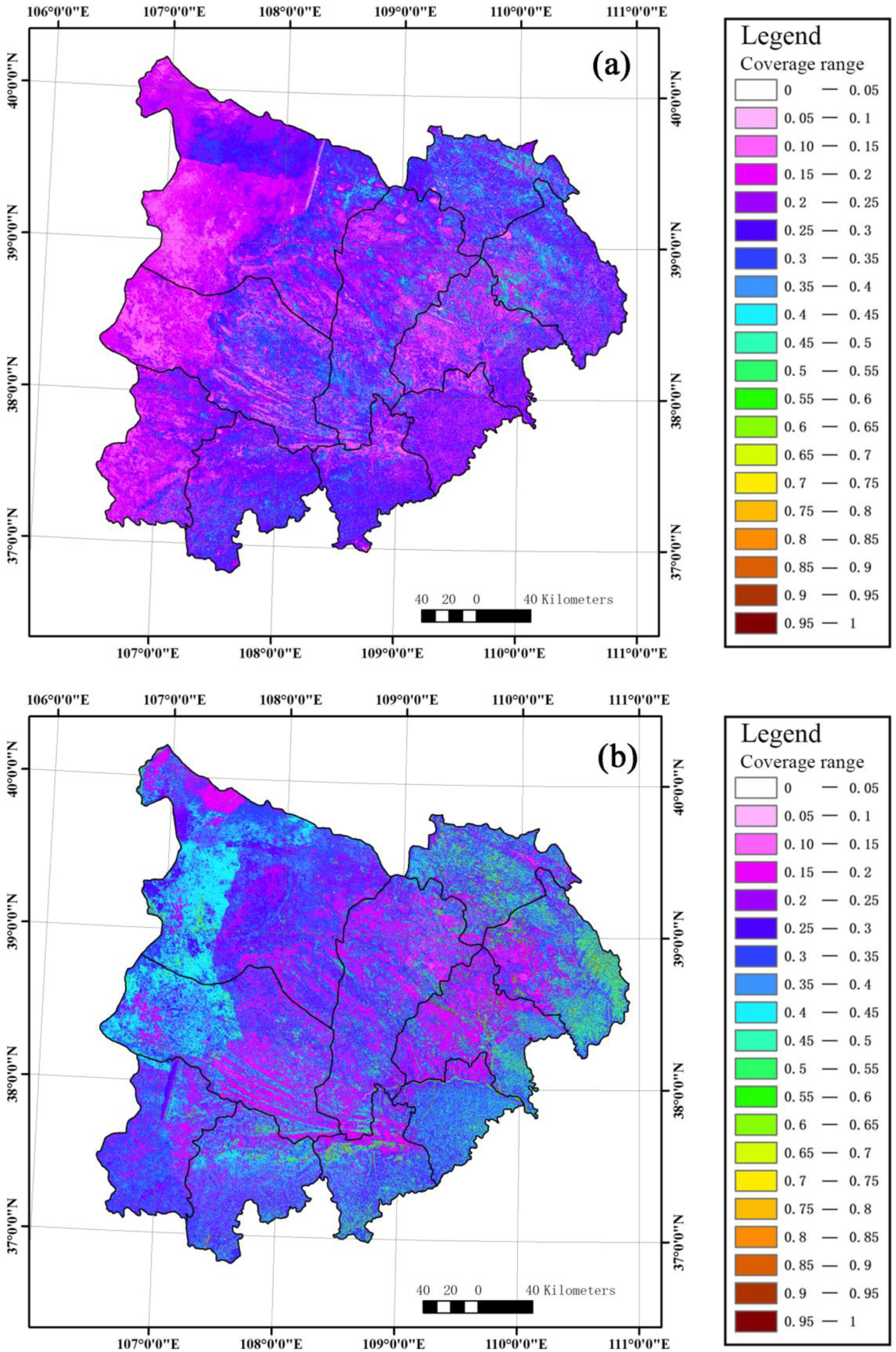
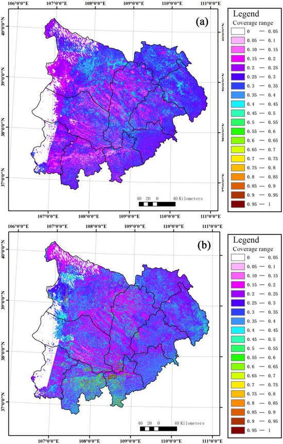
Figure A5.
(a) Non-photosynthetic vegetation coverage at the end of the growing season in 2010. (b) Photosynthetic vegetation coverage at the end of the growing season in 2010.
Figure A5.
(a) Non-photosynthetic vegetation coverage at the end of the growing season in 2010. (b) Photosynthetic vegetation coverage at the end of the growing season in 2010.
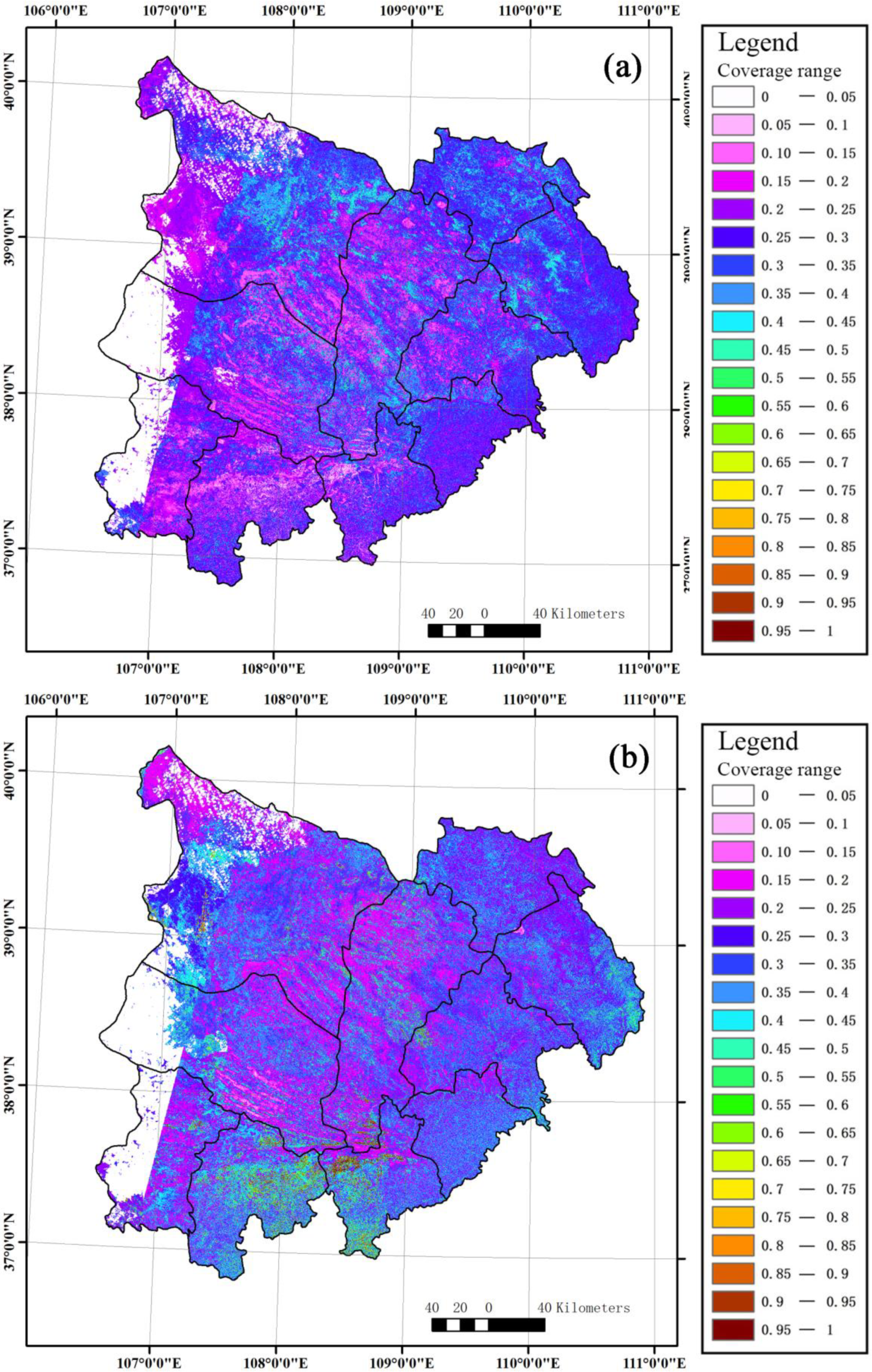
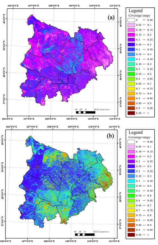
Figure A6.
(a) Non-photosynthetic vegetation coverage at the end of the growing season in 2015. (b) Photosynthetic vegetation coverage at the end of the growing season in 2015.
Figure A6.
(a) Non-photosynthetic vegetation coverage at the end of the growing season in 2015. (b) Photosynthetic vegetation coverage at the end of the growing season in 2015.

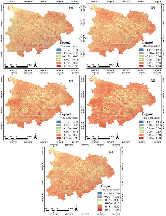
Figure A7.
(a) Response degree of non-photosynthetic vegetation at the end of growing season to total precipitation in 1–9 months. (b) Response degree of non-photosynthetic vegetation at the end of growing season to total precipitation in 10–21 months. (c) Response degree of non-photosynthetic vegetation at the end of growing season to total precipitation in 22–33 months. (d) Response degree of non-photosynthetic vegetation at the end of growing season to total precipitation in 34–45 months. (e) Response degree of non-photosynthetic vegetation at the end of growing season to total precipitation in 46–57 months.
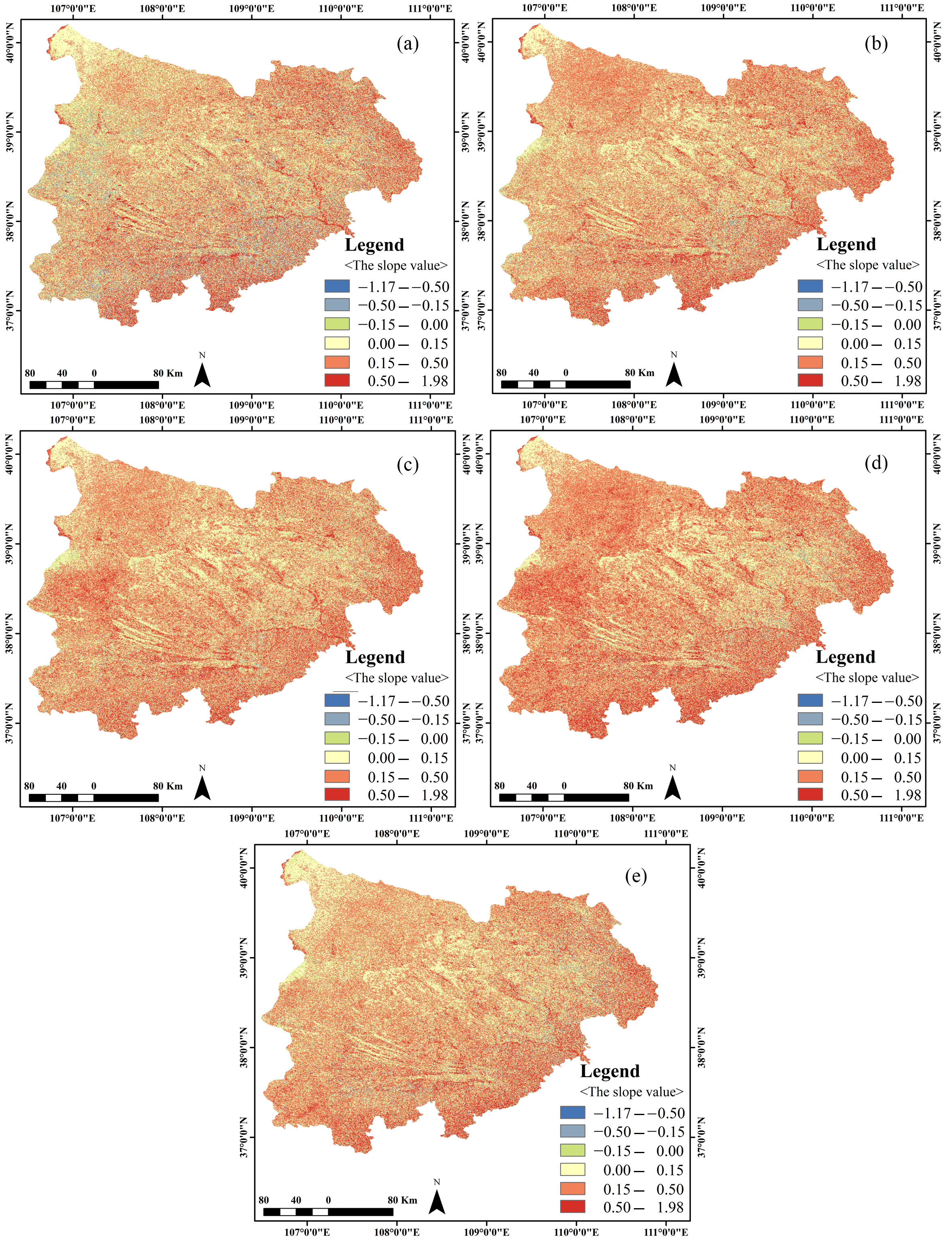
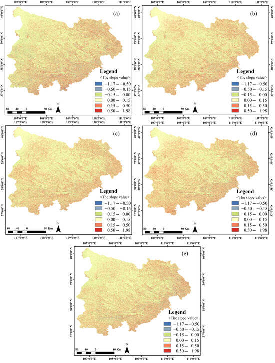
Figure A8.
(a) Response degree of photosynthetic vegetation at the end of growing season to total precipitation in 0–9 months. (b) Response degree of photosynthetic vegetation at the end of growing season to total precipitation in 9–21 months. (c) Response degree of photosynthetic vegetation at the end of growing season to total precipitation in 21–33 months. (d) Response degree of photosynthetic vegetation at the end of growing season to total precipitation in 33–45 months. (e) Response degree of photosynthetic vegetation at the end of growing season to total precipitation in 45–57 months.
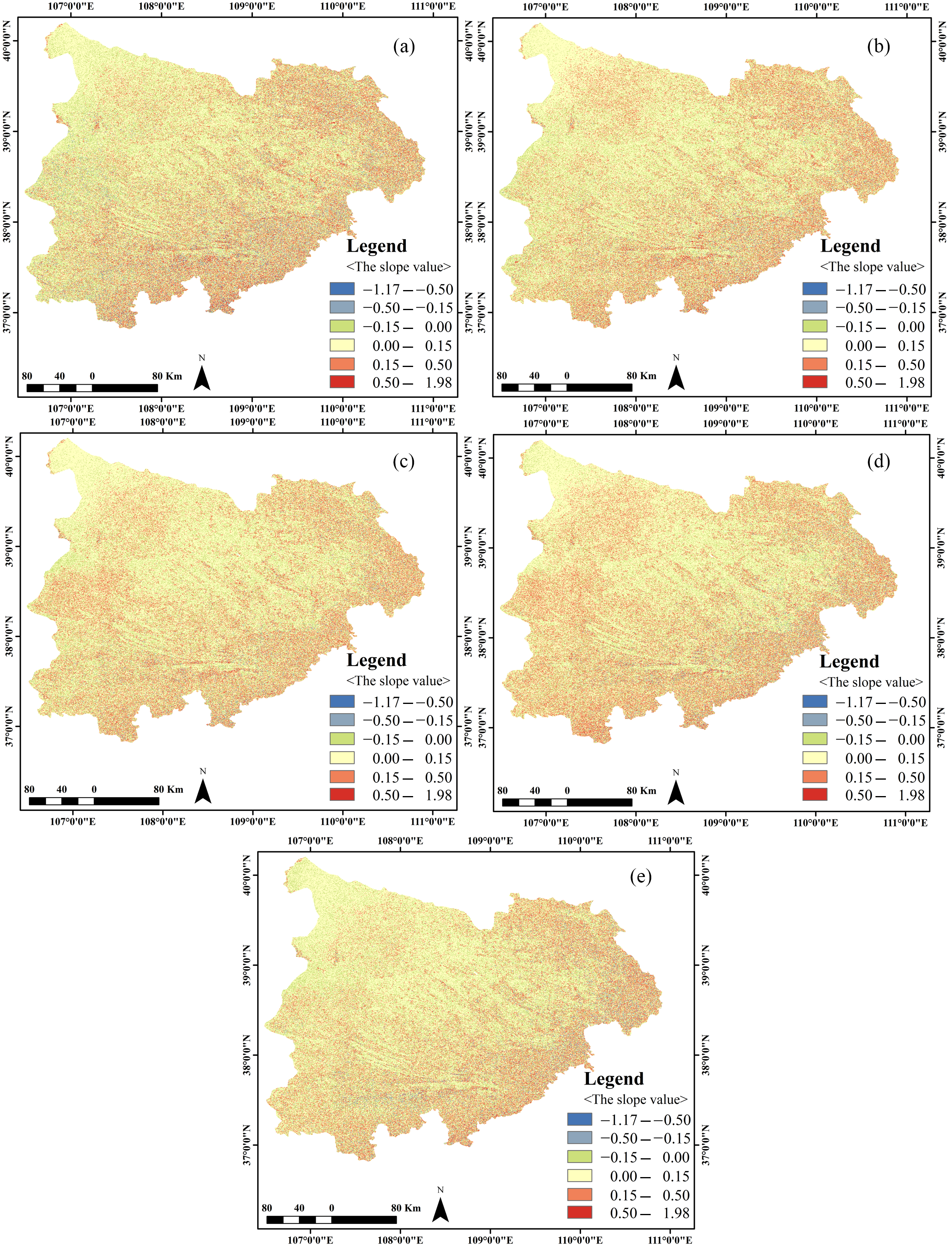
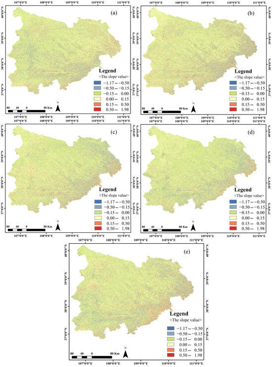
Figure A9.
(a) Response of non-photosynthetic vegetation to 0–9 month mean temperature at the end of growing season. (b) Response of non-photosynthetic vegetation to 9–21 month mean temperature at the end of growing season. (c) Response of non-photosynthetic vegetation to 21–33 month mean temperature at the end of growing season. (d) Response of non-photosynthetic vegetation to 33–45 month mean temperature at the end of growing season. (e) Response of non-photosynthetic vegetation to 45–57 month mean temperature at the end of growing season.
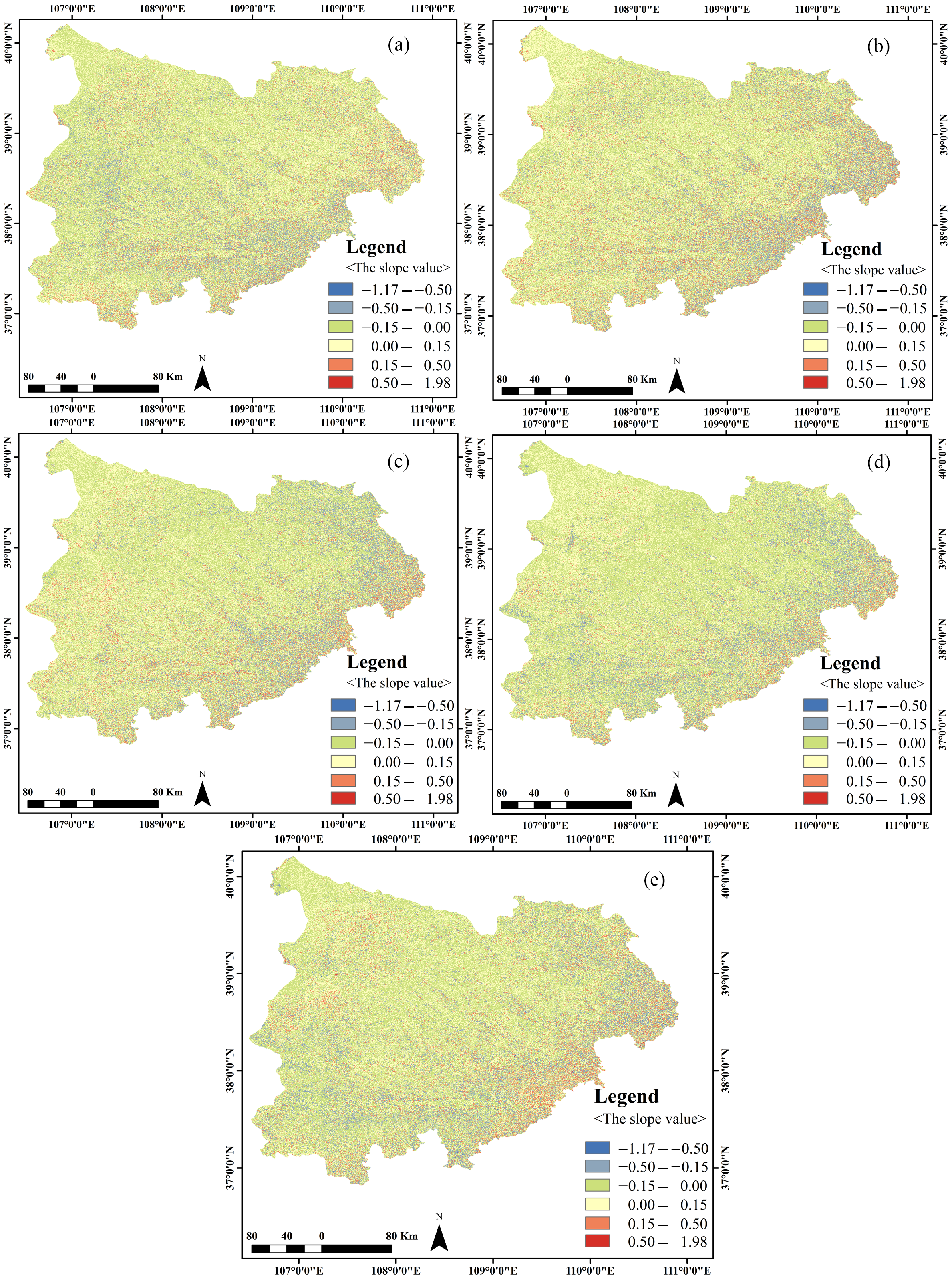
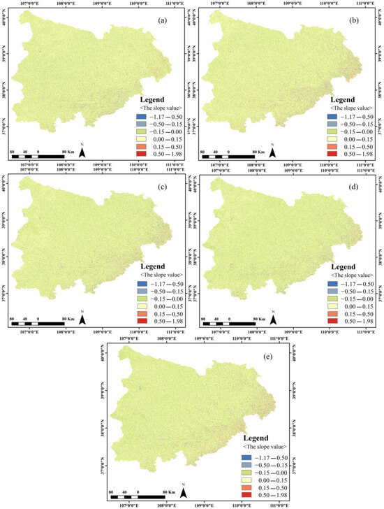
Figure A10.
(a) Response of photosynthetic vegetation to 0–9 month mean temperature at the end of growing season. (b) Response of photosynthetic vegetation to 9–21 month mean temperature at the end of growing season. (c) Response of photosynthetic vegetation to 21–33 month mean temperature at the end of growing season. (d) Response of photosynthetic vegetation to 33–45 month mean temperature at the end of growing season. (e) Response of photosynthetic vegetation to 45–57 month mean temperature at the end of growing season.
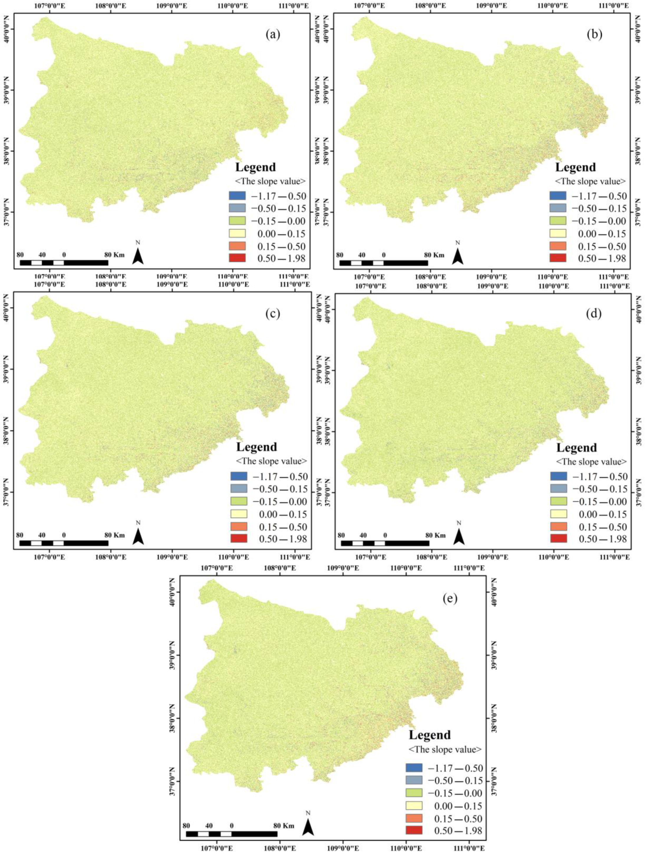
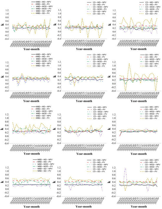
Figure A11.
Time-delay responses of non-photosynthetic and photosynthetic vegetation coverage to monthly precipitation in different desertification types and degrees. Figure note: MBD represents mobile dune desertification; CD represents coppice dune desertification; GD represents Gobi desertification; MD represents mild desertification; MOD represents moderate desertification; and SD represents severe desertification. K is the response degree of NPV and PV to precipitation in the desertification type and degree region.
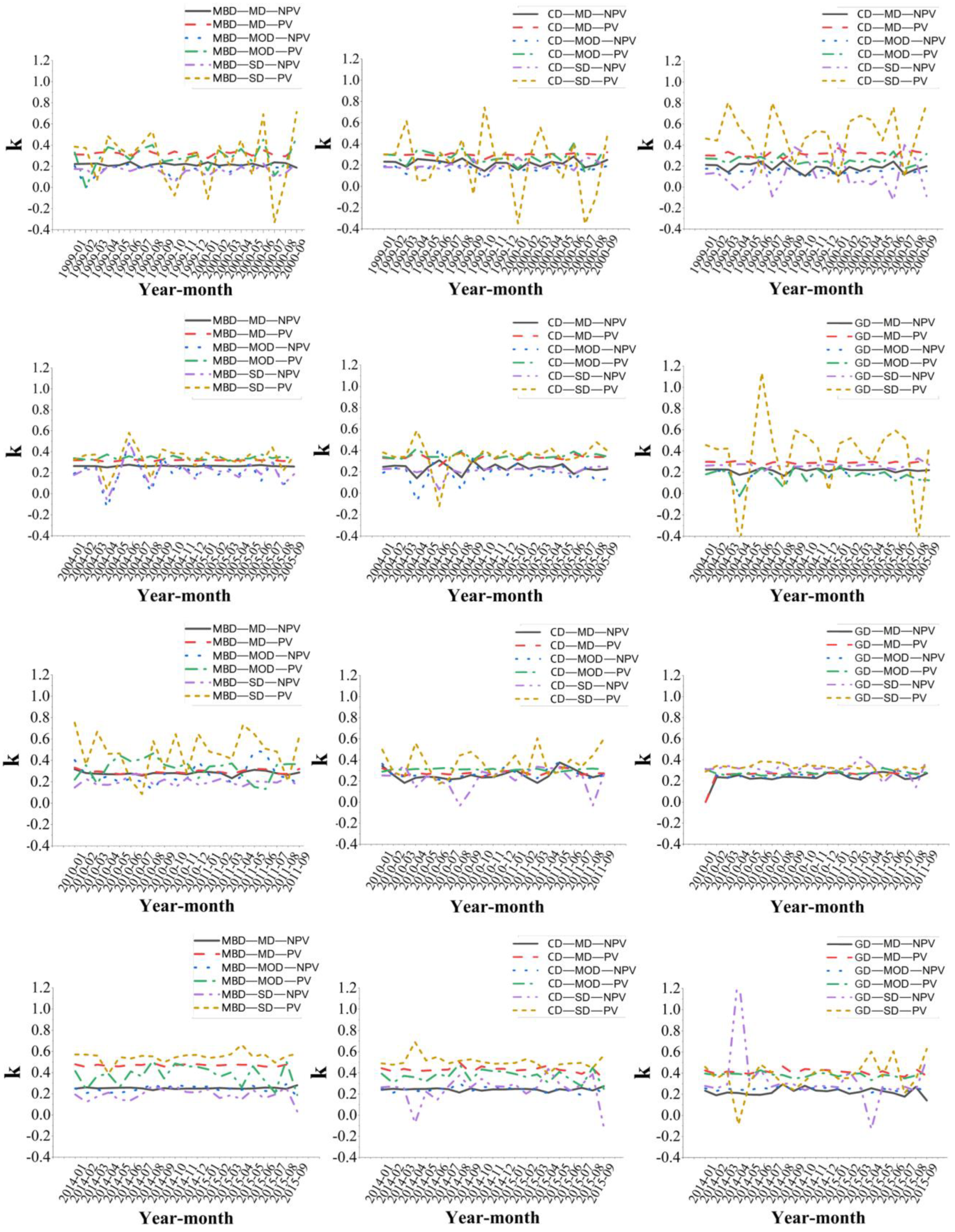
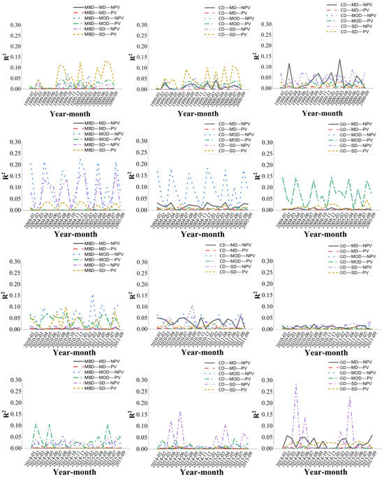
Figure A12.
Time-delay correlation (R2) of non-photosynthetic and photosynthetic vegetation cover with monthly precipitation in different desertification types and degrees. Figure note: MBD represents mobile dune desertification; CD represents coppice dune desertification; GD represents Gobi desertification; MD represents mild desertification; MOD represents moderate desertification; and SD represents severe desertification. R2 is the correlation.
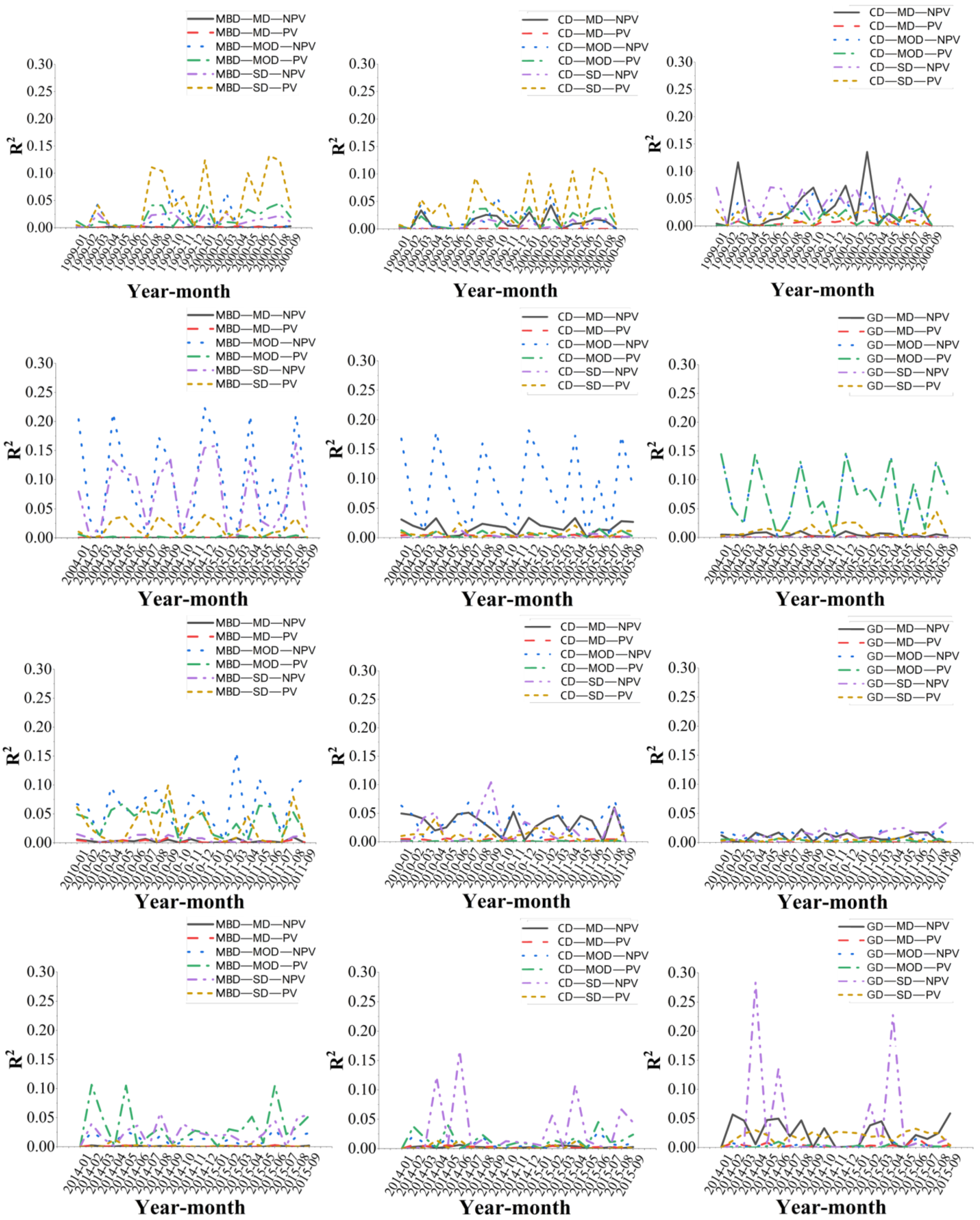
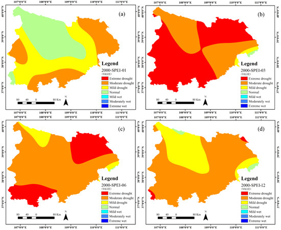
Figure A13.
(a) Spatial distribution map of 1-month SPEI series in September 2000. (b) Spatial distribution map of 3-month SPEI series in September 2000. (c) Spatial distribution map of 9-month SPEI series in September 2000. (d) Spatial distribution map of 12-month SPEI series in September 2000.
Figure A13.
(a) Spatial distribution map of 1-month SPEI series in September 2000. (b) Spatial distribution map of 3-month SPEI series in September 2000. (c) Spatial distribution map of 9-month SPEI series in September 2000. (d) Spatial distribution map of 12-month SPEI series in September 2000.


Figure A14.
(a) Spatial distribution map of 1-month SPEI series in September 2005. (b) Spatial distribution map of 3-month SPEI series in September 2005. (c) Spatial distribution map of 9-month SPEI series in September 2005. (d) Spatial distribution map of 12-month SPEI series in September 2005.
Figure A14.
(a) Spatial distribution map of 1-month SPEI series in September 2005. (b) Spatial distribution map of 3-month SPEI series in September 2005. (c) Spatial distribution map of 9-month SPEI series in September 2005. (d) Spatial distribution map of 12-month SPEI series in September 2005.
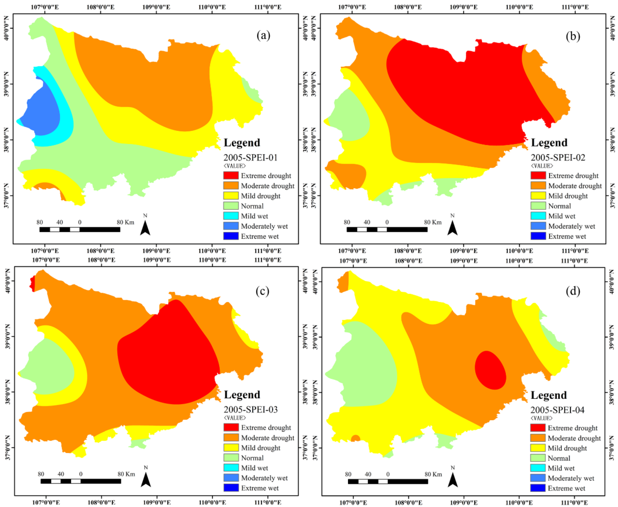

Figure A15.
(a) Spatial distribution map of 1-month SPEI series in September 2010. (b) Spatial distribution map of 3-month SPEI series in September 2010. (c) Spatial distribution map of 9-month SPEI series in September 2010. (d) Spatial distribution map of 12-month SPEI series in September 2010.
Figure A15.
(a) Spatial distribution map of 1-month SPEI series in September 2010. (b) Spatial distribution map of 3-month SPEI series in September 2010. (c) Spatial distribution map of 9-month SPEI series in September 2010. (d) Spatial distribution map of 12-month SPEI series in September 2010.
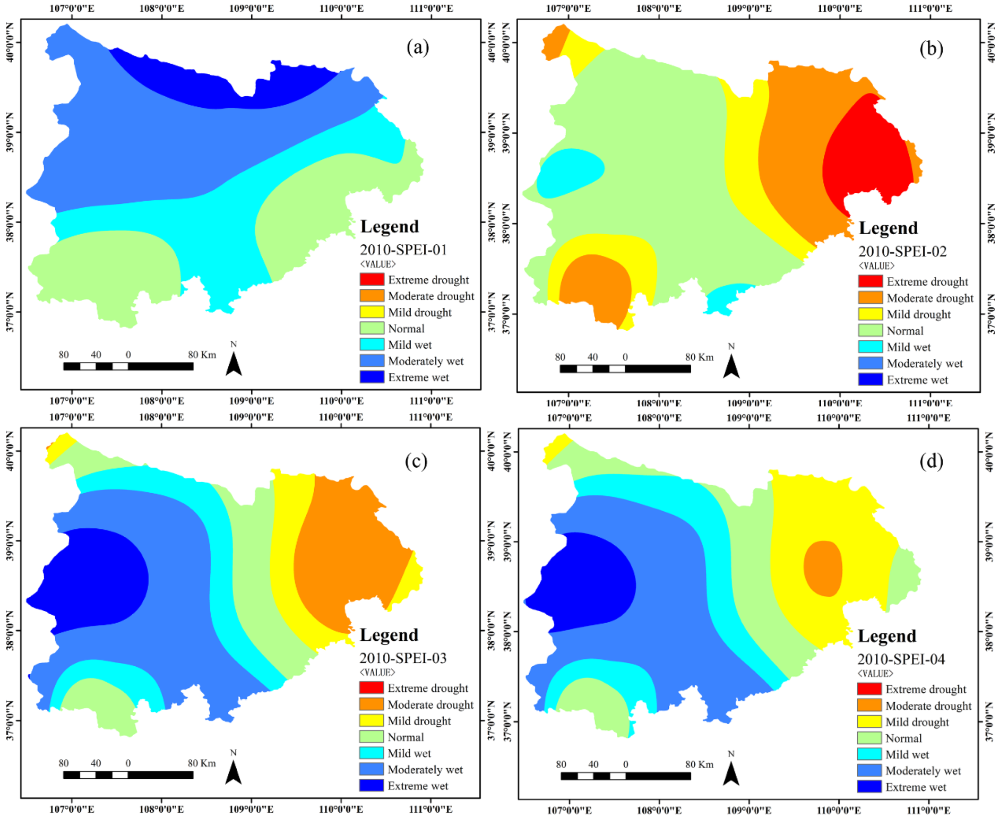
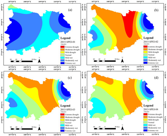
Figure A16.
(a) Spatial distribution map of 1-month SPEI series in September 2015. (b) Spatial distribution map of 3-month SPEI series in September 2015. (c) Spatial distribution map of 9-month SPEI series in September 2015. (d) Spatial distribution map of 12-month SPEI series in September 2015.
Figure A16.
(a) Spatial distribution map of 1-month SPEI series in September 2015. (b) Spatial distribution map of 3-month SPEI series in September 2015. (c) Spatial distribution map of 9-month SPEI series in September 2015. (d) Spatial distribution map of 12-month SPEI series in September 2015.

References
- Li, C.; Fu, B.; Wang, S.; Stringer, L.C.; Wang, Y.; Li, Z.; Liu, Y.; Zhou, W. Drivers and impacts of changes in China’s drylands. Nat. Rev. Earth Environ. 2021, 2, 858–873. [Google Scholar] [CrossRef]
- Ahlström, A.; Raupach, M.R.; Schurgers, G.; Smith, B.; Arneth, A.; Jung, M.; Reichstein, M.; Canadell, J.G.; Friedlingstein, P.; Jain, A.K.; et al. The dominant role of semi-arid ecosystems in the trend and variability of the land CO2 sink. Science 2015, 348, 895–899. [Google Scholar] [CrossRef] [PubMed]
- Zhang, L.; Xiao, J.; Zheng, Y.; Li, S.; Zhou, Y. Increased carbon uptake and water use efficiency in global semi-arid ecosystems. Environ. Res. Lett. 2020, 15, 034022. [Google Scholar] [CrossRef]
- Smith, W.K.; Reed, S.C.; Cleveland, C.C.; Ballantyne, A.P.; Anderegg, W.R.; Wieder, W.R.; Liu, Y.Y.; Running, S.W. Large divergence of satellite and Earth system model estimates of global terrestrial CO2 fertilization. Nat. Clim. Change 2016, 6, 306–310. [Google Scholar] [CrossRef]
- Guerschman, J.P.; Hill, M.J.; Renzullo, L.J.; Barrett, D.J.; Marks, A.S.; Botha, E.J. Estimating fractional cover of photosynthetic vegetation, non-photosynthetic vegetation and bare soil in the Australian tropical savanna region upscaling the EO-1 Hyperion and MODIS sensors. Remote Sens. Environ. 2009, 113, 928–945. [Google Scholar] [CrossRef]
- Guo, Z.C.; Wang, T.; Liu, S.; Kang, W.; Chen, X.; Feng, K.; Zhi, Y. Comparison of the backpropagation network and the random forest algorithm based on sampling distribution effects consideration for estimating nonphotosynthetic vegetation cover. Int. J. Appl. Earth Obs. Geoinf. 2021, 104, 102573. [Google Scholar]
- Guerschman, J.P.; Hill, M.J.; Leys, J.; Heidenreich, S. Vegetation cover dependence on accumulated antecedent precipitation in Australia: Relationships with photosynthetic and non-photosynthetic vegetation fractions. Remote Sens. Environ. 2020, 240, 111670. [Google Scholar] [CrossRef]
- Qu, H.; Zhao, X.; Lian, J.; Tang, X.; Wang, X.; Medina-Roldán, E. Increasing Precipitation Interval Has More Impacts on Litter Mass Loss Than Decreasing Precipitation Amount in Desert Steppe. Front. Environ. Sci. 2020, 8, 88. [Google Scholar] [CrossRef]
- Singh, K.; Trivedi, P.; Singh, G.; Singh, B.; Patra, D.D. Effect of different leaf litters on carbon, nitrogen and microbial activities of sodic soils. Land Degrad. Dev. 2016, 27, 1215–1226. [Google Scholar] [CrossRef]
- Jia, C.; Liu, Y.; He, H.; Miao, H.T.; Huang, Z.; Zheng, J.; Han, F.; Wu, G.L. Formation of litter crusts and its multifunctional ecological effects in a desert ecosystem. Ecosphere 2018, 9, e02196. [Google Scholar] [CrossRef]
- Liu, Y.; Cui, Z.; Huang, Z.; Miao, H.T.; Wu, G.L. The influence of litter crusts on soil properties and hydrological processes in a sandy ecosystem. Hydrol. Earth Syst. Sci. 2019, 23, 2481–2490. [Google Scholar] [CrossRef]
- Liu, X.Z.; Liu, Y.; Zhang, L.; Yin, R.; Wu, G.L. Bacterial contributions of bio-crusts and litter crusts to nutrient cycling in the Mu Us Sandy Land. Catena 2021, 199, 105090. [Google Scholar] [CrossRef]
- Zuazo, V.H.D.; Pleguezuelo, C.R.R. Soil-Erosion and Runoff Prevention by Plant Covers: A Review. In Sustainable Agriculture; Springer: Dordrecht, The Netherlands, 2009; pp. 785–811. [Google Scholar]
- Zhang, X.T.; Bi, J.; Zhu, D.; Meng, Z. Seasonal variation of net ecosystem carbon exchange and gross primary production over a Loess Plateau semi-arid grassland of northwest China. Sci. Rep. 2024, 14, 2916. [Google Scholar] [CrossRef]
- Zhang, F.Y.; Biederman, J.A.; Pierce, N.A.; Potts, D.L.; Devine, C.J.; Hao, Y.; Smith, W.K. Precipitation temporal repackaging into fewer, larger storms delayed seasonal timing of peak photosynthesis in a semi-arid grassland. Funct. Ecol. 2022, 36, 646–658. [Google Scholar] [CrossRef]
- Guerschman, J.P.; Scarth, P.F.; McVicar, T.R.; Renzullo, L.J.; Malthus, T.J.; Stewart, J.B.; Rickards, J.E.; Trevithick, R. Assessing the effects of site heterogeneity and soil properties when unmixing photosynthetic vegetation, non-photosynthetic vegetation and bare soil fractions from Landsat and MODIS data. Remote Sens. Environ. 2015, 161, 12–26. [Google Scholar] [CrossRef]
- Rickards, J.; Stewart, J.; McPhee, R.; Randall, L. Australian ground cover reference sites database: User guide for PostGIS. Victoria 2012, 48, 20. [Google Scholar]
- Rouse, J.W., Jr.; Haas, R.H.; Schell, J.; Deering, D. Monitoring the Vernal Advancement and Retrogradation (Green Wave Effect) of Natural Vegetation; Technical Report. 1973. Available online: https://ntrs.nasa.gov/citations/19740022555 (accessed on 23 May 2023).
- Liu, H.Q.; Huete, A. A feedback based modification of the ndvi to minimize canopy background and atmospheric noise. IEEE Trans. Geosci. Remote Sens. 1995, 33, 814. [Google Scholar] [CrossRef]
- Qi, J.; Chehbouni, A.; Huete, A.R.; Kerr, Y.H.; Sorooshian, S. A modified soil adjusted vegetation index. Remote Sens. Environ. 1994, 48, 119–126. [Google Scholar] [CrossRef]
- Cao, X.; Chen, J.; Matsushita, B.; Imura, H. Developing a MODIS-based index to discriminate dead fuel from photosynthetic vegetation and soil background in the Asian steppe area. Int. J. Remote Sens. 2010, 31, 1589–1604. [Google Scholar] [CrossRef]
- Gitelson, A.A.; Viña, A.; Ciganda, V.; Rundquist, D.C.; Arkebauer, T.J. Remote estimation of canopy chlorophyll content in crops. Geophys. Res. Lett. 2005, 32, L08403. [Google Scholar] [CrossRef]
- McNairn, H.; Protz, R. Mapping corn residue cover on agricultural fields in Oxford County, Ontario, using Thematic Mapper. Can. J. Remote Sens. 1993, 19, 152–159. [Google Scholar] [CrossRef]
- Wang, G.; Wang, J.; Han, L.; Chai, G.; Wang, Z. Estimating fractional cover of non-photosynthetic vegetation using field spectral to simulate Landsat-8 OLI. Int. J. Geogr. Inf. Sci. 2018, 20, 1667–1678. [Google Scholar]
- Okin, G.S. Relative spectral mixture analysis—A multitemporal index of total vegetation cover. Remote Sens. Environ. 2007, 106, 467–479. [Google Scholar] [CrossRef]
- Okin, G.S.; Clarke, K.D.; Lewis, M.M. Comparison of methods for estimation of absolute vegetation and soil fractional cover using MODIS normalized BRDF-adjusted reflectance data. Remote Sens. Environ. 2013, 130, 266–279. [Google Scholar] [CrossRef]
- Niu, F.R.; Duan, D.; Chen, J.; Xiong, P.; Zhang, H.; Wang, Z.; Xu, B. Eco-Physiological Responses of Dominant Species to Watering in a Natural Grassland Community on the Semi-Arid Loess Plateau of China. Front. Plant Sci. 2016, 7, 663. [Google Scholar] [CrossRef]
- Lin, Y.; Chen, Z.; Yang, M.; Chen, S.P.; Gao, Y.H.; Liu, R.; Hao, Y.; Xin, X.; Zhou, L.; Yu, G.R. Temporal and spatial variations of ecosystem photosynthetic parameters in arid and semi-arid areas of China and its influencing factors. Chin. J. Plant Ecol. 2022, 46, 1461. [Google Scholar] [CrossRef]
- Zhang, C.; Wang, Y.; Yan, D.; Guo, R.; Shuai, H.E.; Miao, L.; Li, X. Analysis of Climate Change and Drought Trend in Desert Steppe of Inner Mongolia. J. Irrig. Drain. 2020, 39, 5. [Google Scholar] [CrossRef]
- Zhao, D.S.; Gao, X.; Wu, S.H. Nonuniform variations of precipitation and temperature across China over the period 1960–2015. Int. J. Climatol. 2021, 41, 316–327. [Google Scholar] [CrossRef]
- Luo, Y.Q.; Zhou, J.; Yue, X.F.; Ding, J.P. Effect of precipitation frequency on litter decomposition of three annual species (Setaria viridis, Artemisia sacrorum, and Chenopodium acuminatum) in a semi-arid sandy grassland of northeastern China. Arid Land Res. Manag. 2021, 35, 397–413. [Google Scholar] [CrossRef]
- Zhang, Y.J.; Gan, Z.T.; Li, R.J.; Wang, R.; Li, N.N.; Zhao, M.; Du, L.L.; Guo, S.L.; Jiang, J.S.; Wang, Z.Q. Litter production rates and soil moisture influences interannual variability in litter respiration in the semi-arid Loess Plateau, China. J. Arid Environ. 2016, 125, 43–51. [Google Scholar] [CrossRef]
- Xu, H.; Wang, X.; Zhao, C. Drought sensitivity of vegetation photosynthesis along the aridity gradient in northern China. Int. J. Appl. Earth Obs. Geoinf. 2021, 102, 102418. [Google Scholar] [CrossRef]
- Gu, Q.; Wei, J.; Luo, S.C.; Ma, M.G.; Tang, X.G. Potential and environmental control of carbon sequestration in major ecosystems across arid and semi-arid regions in China. Sci. Total Environ. 2018, 645, 796–805. [Google Scholar] [CrossRef] [PubMed]
- Nakano, T.; Nemoto, M.; Shinoda, M. Environmental controls on photosynthetic production and ecosystem respiration in semi-arid grasslands of Mongolia. Agric. For. Meteorol. 2008, 148, 1456–1466. [Google Scholar] [CrossRef]
- Yuanyuan, Z.; Guodong, D.; Guanglei, G.; Le, P.; Xiao, C. Regionalization for Aeolian Desertification Control in the Mu Us Sandy Land Region, China. J. Desert Res. 2017, 37, 635. [Google Scholar]
- Xu, C.; Ke, Y.G.; Zhou, W.; Luo, W.T.; Ma, W.; Song, L.; Smith, M.D.; Hoover, D.L.; Wilcox, K.R.; Fu, W.; et al. Resistance and resilience of a semi-arid grassland to multi-year extreme drought. Ecol. Indic. 2021, 131, 108139. [Google Scholar] [CrossRef]
- Shumack, S.; Fisher, A.; Hesse, P.P. Refining medium resolution fractional cover for arid Australia to detect vegetation dynamics and wind erosion susceptibility on longitudinal dunes. Remote Sens. Environ. 2021, 265, 112647. [Google Scholar] [CrossRef]
- Zhang, C.; Filella, I.; Liu, D.J.; Ogaya, R.; Llusià, J.; Asensio, D.; Peñuelas, J. Photochemical Reflectance Index (PRI) for Detecting Responses of Diurnal and Seasonal Photosynthetic Activity to Experimental Drought and Warming in a Mediterranean Shrubland. Remote Sens. 2017, 9, 1189. [Google Scholar] [CrossRef]
- Mengoli, G.; Agustí-Panareda, A.; Boussetta, S.; Harrison, S.P.; Trotta, C.; Prentice, I.C. Ecosystem Photosynthesis in Land-Surface Models: A First-Principles Approach Incorporating Acclimation. J. Adv. Model. Earth Syst. 2022, 14, e2021MS002767. [Google Scholar] [CrossRef]
- Cai, A.; Liang, G.; Yang, W.; Zhu, J.; Han, T.; Zhang, W.; Xu, M. Patterns and driving factors of litter decomposition across Chinese terrestrial ecosystems. J. Clean. Prod. 2021, 278, 123964. [Google Scholar] [CrossRef]
- Yue, K.; Peng, C.H.; Yang, W.Q.; Peng, Y.; Fang, J.M.; Wu, F.Z. Study type and plant litter identity modulating the response of litter decomposition to warming, elevated CO2, and elevated O3: A meta-analysis. J. Geophys. Res. Biogeosciences 2015, 120, 441–451. [Google Scholar] [CrossRef]
- Hong, C.; Zhen, Z.; Lang, X.; Yi, W.; Si, W.; Yi, H.; Zhen, X.; Chun, Y.; He, W. Flora of China; Science Press: Beijing, China, 1998. [Google Scholar]
- Zichen, G.; Shulin, L.; Wenping, K.; Xiang, C.; Xueqin, Z. Change trend of vegetation coverage in the Mu Us Sandy Region from 2000 to 2015. J. Desert Res. 2018, 38, 1099. [Google Scholar]
- Poursanidis, D.; Chrysoulakis, N.; Mitraka, Z. Landsat 8 vs. Landsat 5: A comparison based on urban and pen-urban land cover mapping. Int. J. Appl. Earth Obs. Geoinf. 2015, 35, 259–269. [Google Scholar] [CrossRef]
- Mishra, N.; Helder, D.; Barsi, J.; Markham, B. Continuous calibration improvement in solar reflective bands: Landsat 5 through Landsat 8. Remote Sens. Environ. 2016, 185, 7–15. [Google Scholar] [CrossRef] [PubMed]
- Vicente-Serrano, S.M.; Beguería, S.; López-Moreno, J.I. A Multiscalar Drought Index Sensitive to Global Warming: The Standardized Precipitation Evapotranspiration Index. J. Clim. 2010, 23, 1696–1718. [Google Scholar] [CrossRef]
- Clark, R.N. Remote Sensing for the Earth Sciences: Manual of Remote Sensing. In Spectroscopy of Rocks and Minerals, and Principles of Spectroscopy; Rencz, A.N., Ed.; John and Wiley and Sons: New York, NY, USA, 1993. [Google Scholar]
- Kokaly, R.F.; Couvillion, B.R.; Holloway, J.M.; Roberts, D.A.; Ustin, S.L.; Peterson, S.H.; Khanna, S.; Piazza, S.C. Spectroscopic remote sensing of the distribution and persistence of oil from the Deepwater Horizon spill in Barataria Bay marshes. Remote Sens. Environ. 2013, 129, 210–230. [Google Scholar] [CrossRef]
- Bannari, A.; PacheCo, A.; Staenz, K.; McNairn, H.; Omari, K. Estimating and mapping crop residues cover on agricultural lands using hyperspectral and IKONOS data. Remote Sens. Environ. 2006, 104, 447–459. [Google Scholar] [CrossRef]
- Daughtry, C.S.T. Discriminating crop residues from soil by shortwave infrared reflectance. Agron. J. 2001, 93, 125–131. [Google Scholar] [CrossRef]
- Hively, W.D.; Lamb, B.T.; Daughtry, C.S.T.; Shermeyer, J.; McCarty, G.W.; Quemada, M. Mapping Crop Residue and Tillage Intensity Using WorldView-3 Satellite Shortwave Infrared Residue Indices. Remote Sens. 2018, 10, 1657. [Google Scholar] [CrossRef]
- Henry, H.A.L.; Moise, E.R.D. Grass litter responses to warming and N addition: Temporal variation in the contributions of litter quality and environmental effects to decomposition. Plant Soil 2015, 389, 35–43. [Google Scholar] [CrossRef]
- Shen, Y.; Chen, W.Q.; Yang, G.W.; Yang, X.; Liu, N.; Sun, X.; Chen, J.S.; Zhang, Y.J. Can litter addition mediate plant productivity responses to increased precipitation and nitrogen deposition in a typical steppe? Ecol. Res. 2016, 31, 579–587. [Google Scholar] [CrossRef]
- Xianghan, L. Soil Moisture Mechanism in Fixed Sand Dunes of Artemisia Ordosica Community in Mu Us Sandy Land. Environ. Resour. Ecol. J. 2024, 8, 114–127. [Google Scholar]
- Tang, Y.K.; Jiang, J.; Chen, C.; Chen, Y.M.; Wu, X. Rainfall pulse response of carbon fluxes in a temperate grass ecosystem in the semiarid Loess Plateau. Ecol. Evol. 2018, 8, 11179–11189. [Google Scholar] [CrossRef] [PubMed]
- Cui, X.; Du, Z.; Wang, Y. Photosynthetic characteristics of a semi-arid sandy grassland community in inner mongolia. Chin. J. Plant Ecol. 2000, 24, 541. [Google Scholar]
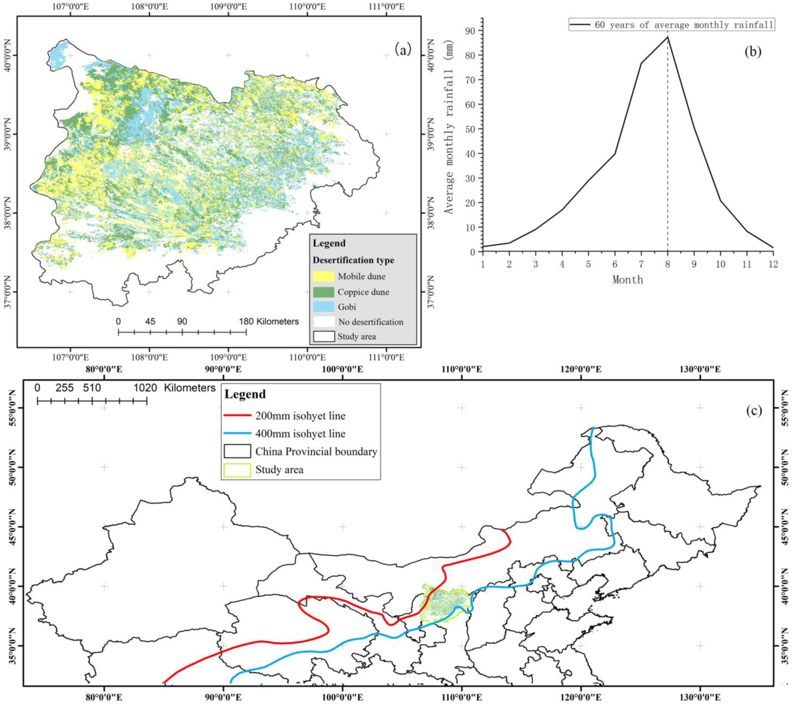
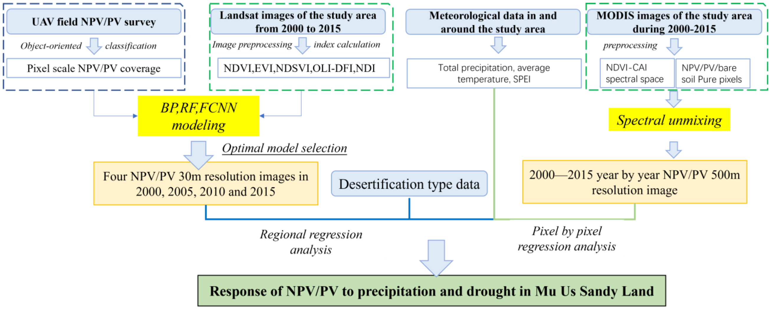
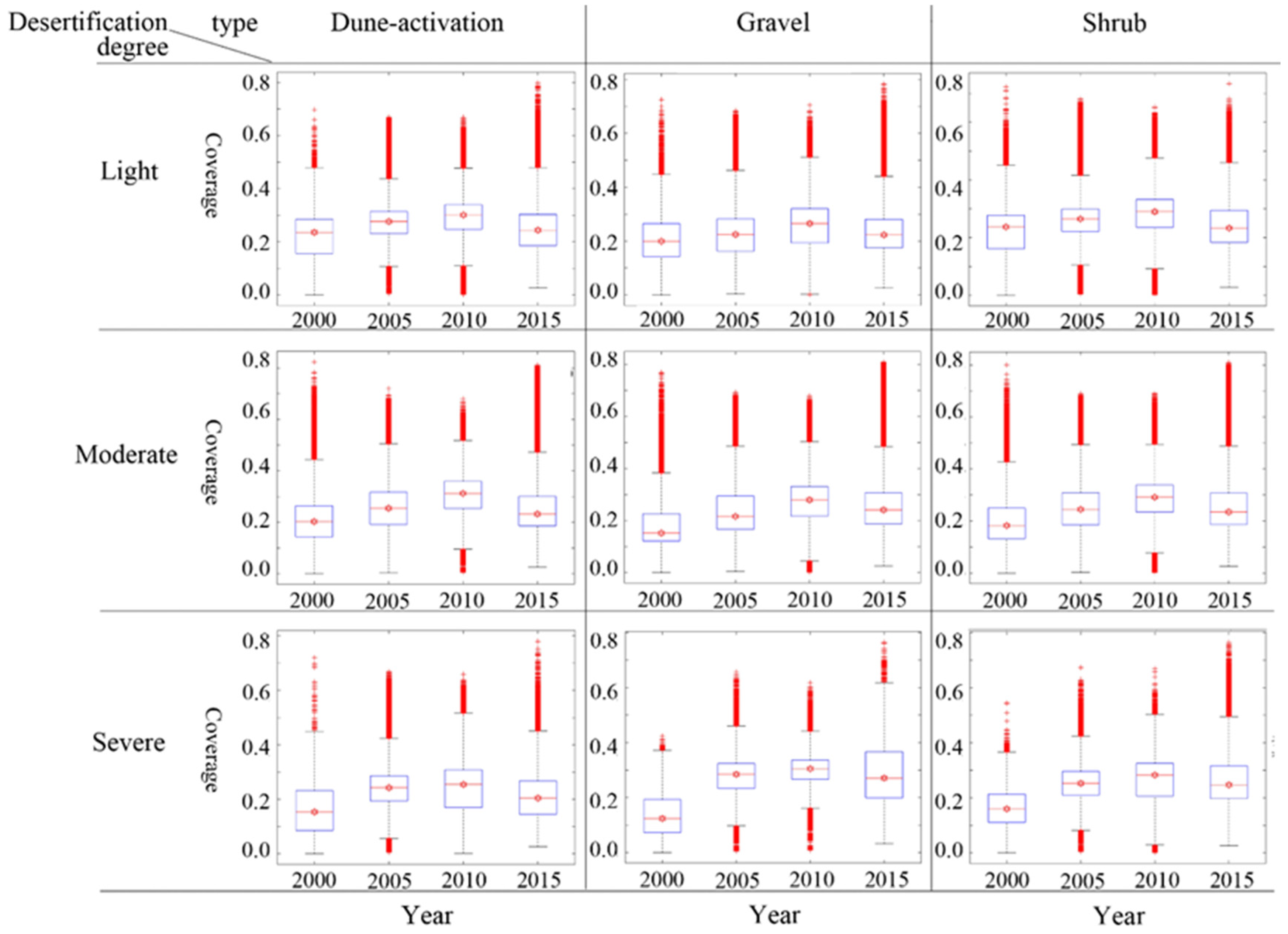
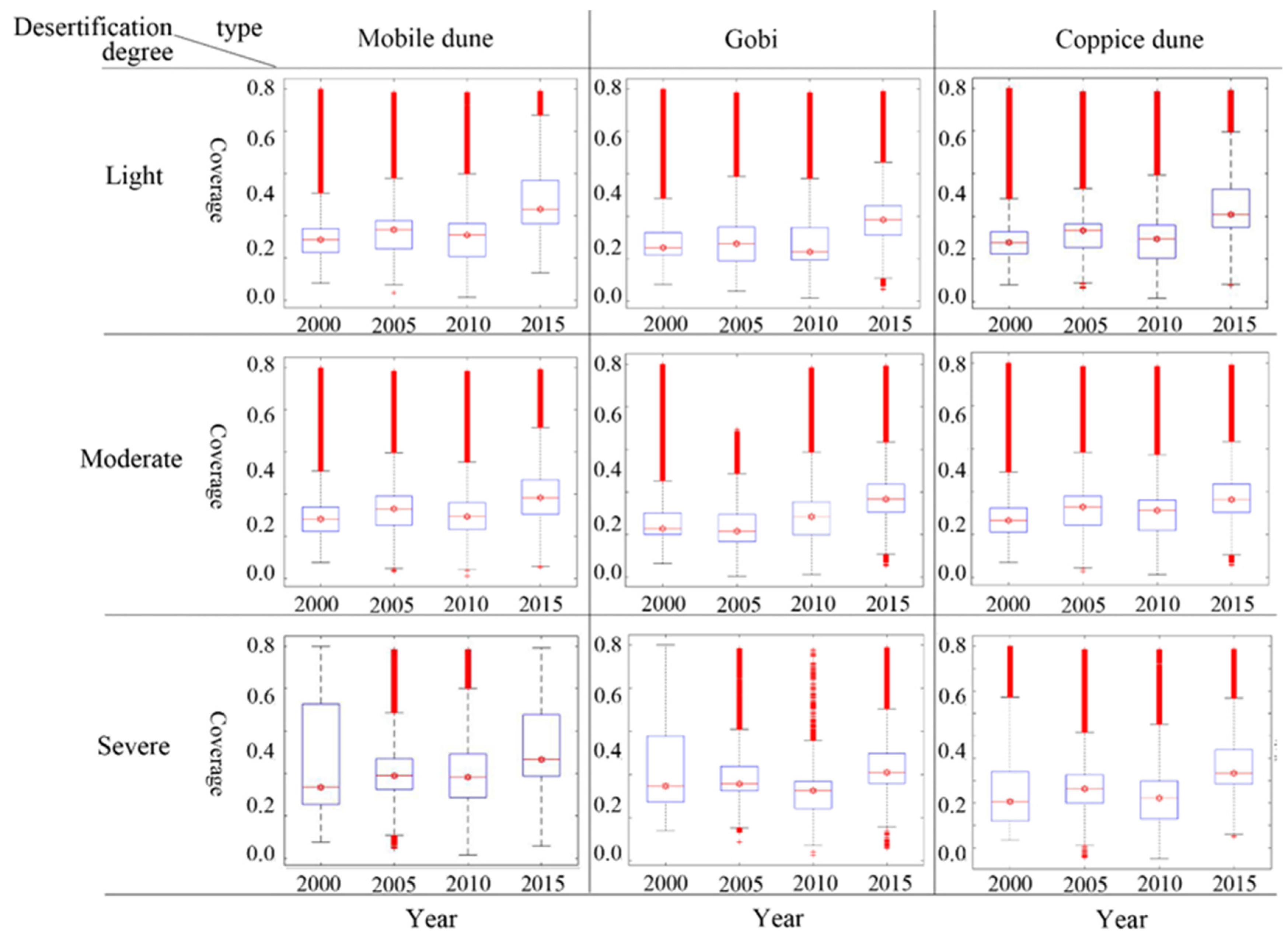
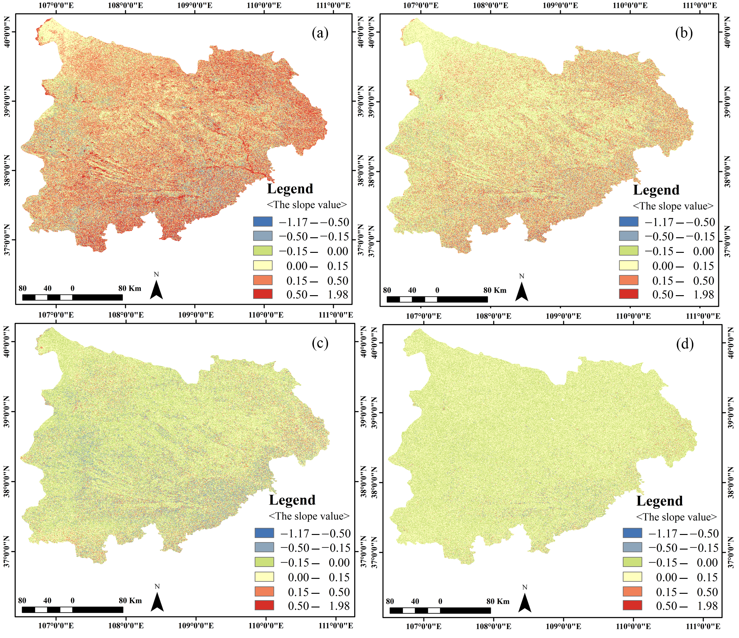
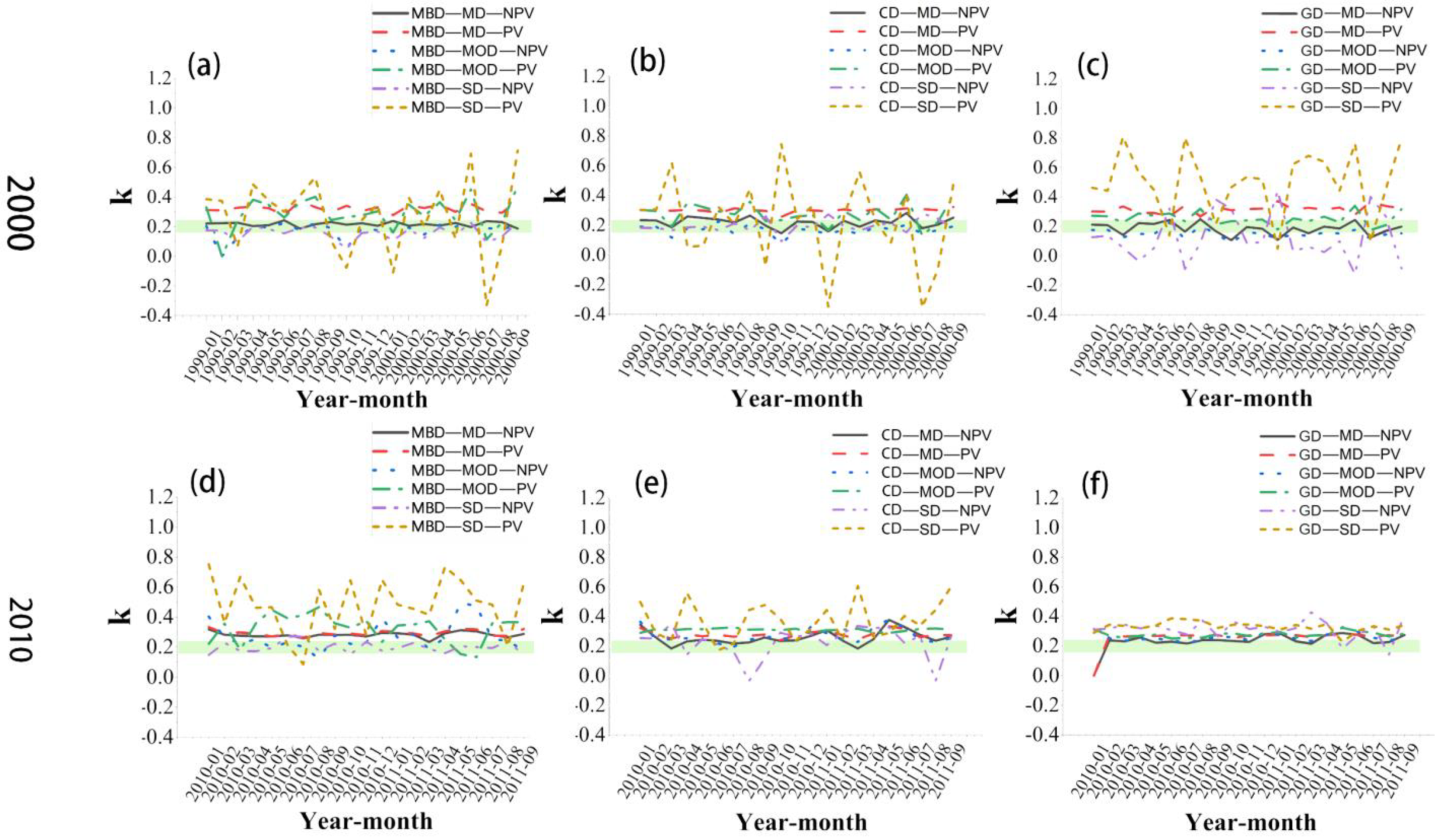
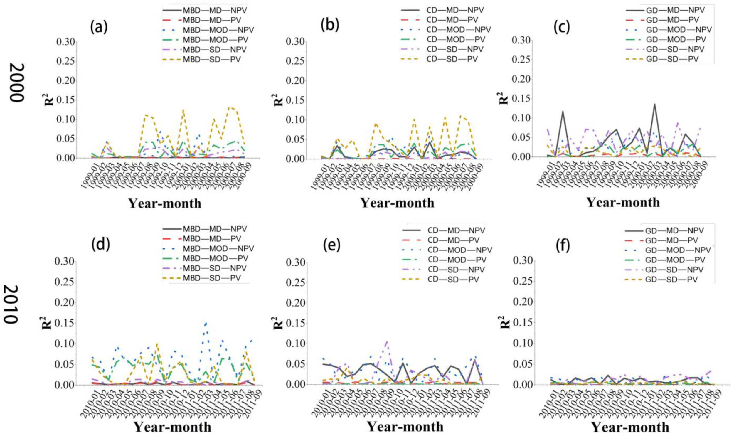
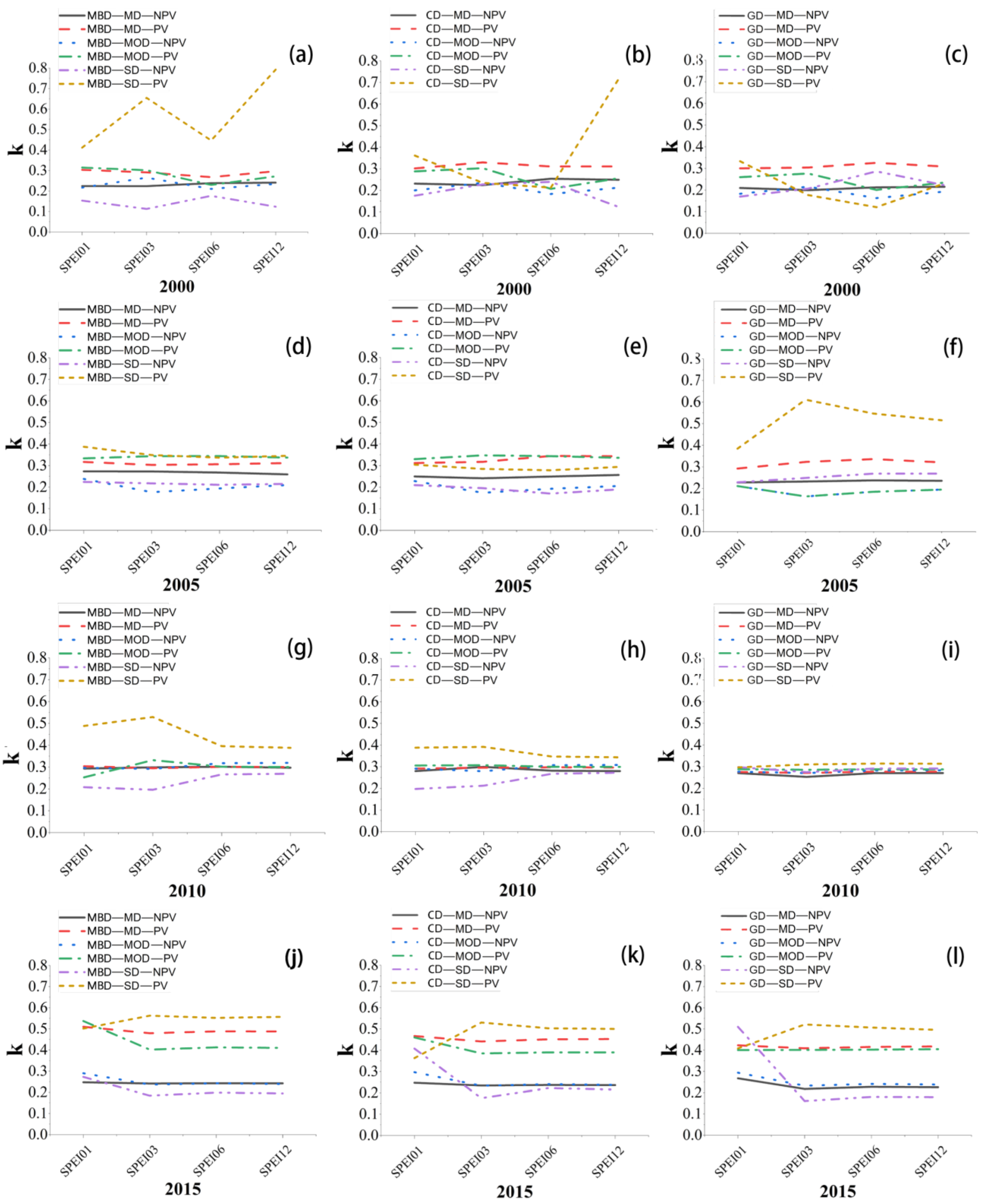
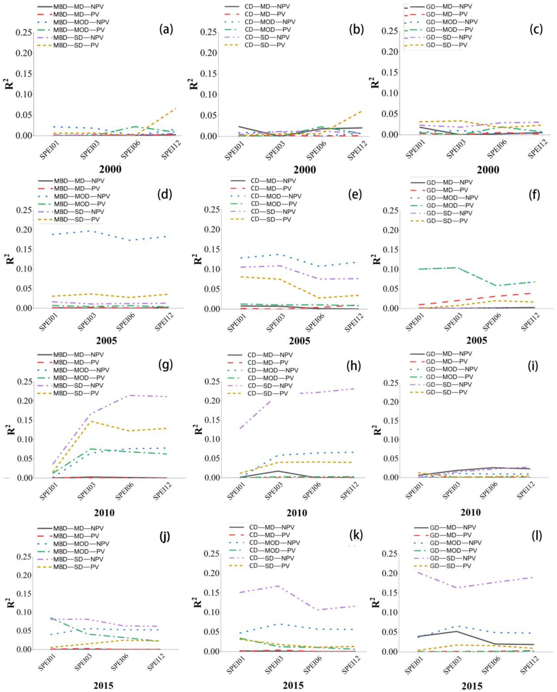

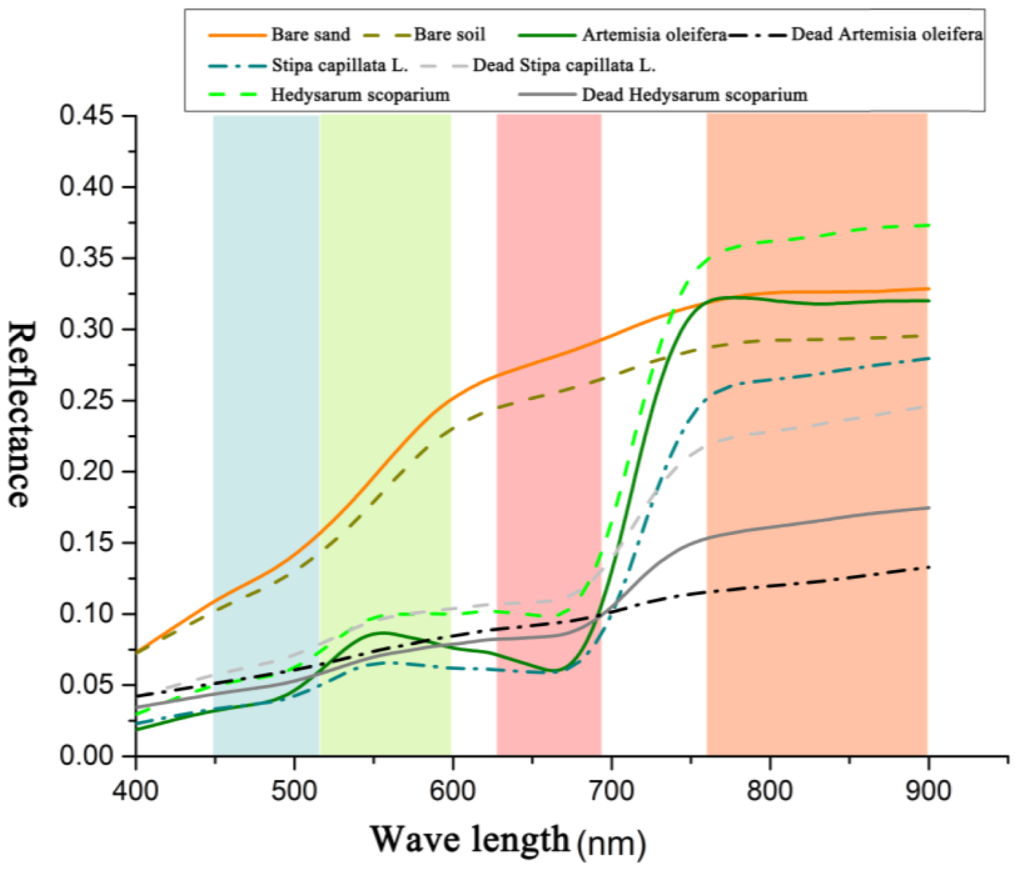
Disclaimer/Publisher’s Note: The statements, opinions and data contained in all publications are solely those of the individual author(s) and contributor(s) and not of MDPI and/or the editor(s). MDPI and/or the editor(s) disclaim responsibility for any injury to people or property resulting from any ideas, methods, instructions or products referred to in the content. |
© 2024 by the authors. Licensee MDPI, Basel, Switzerland. This article is an open access article distributed under the terms and conditions of the Creative Commons Attribution (CC BY) license (https://creativecommons.org/licenses/by/4.0/).