Advancing Skarn Iron Ore Detection through Multispectral Image Fusion and 3D Convolutional Neural Networks (3D-CNNs)

Abstract

This study explores novel techniques to improve the detection accuracy of skarn iron deposits using advanced image-processing methodologies. Leveraging the capabilities of ASTER image, band ratio (BR) images, and principal component analysis (PCA) alongside the power of 3D convolutional neural networks (3D-CNNs), the research aims to enhance the precision and efficiency of ore detection in complex geological environments. The proposed method employs a specific 3D-CNN architecture accepting input as a 7 × 7 × C image patch, where C represents the combined number of selected ASTER image bands, principal component (PC) bands, and computed BR images. To evaluate the accuracy of the proposed method, five distinct image band combinations, including the proposed band combination, were tested and evaluated based on the overall accuracy (OA), average accuracy (AA), and kappa coefficient. The results demonstrated that while the incorporation of BR images alongside ASTER bands initially seemed promising, it introduced significant confusion in certain classifications, leading to unexpected misclassification rates. Surprisingly, utilizing solely ASTER bands as input parameters yielded higher accuracy rates (OA = 93.13%, AA = 91.96%, kappa = 90.91%) compared with scenarios involving the integration with band ratios (OA = 87.02%, AA = 79.15, kappa = 82.60%) or the integration of BR images to PC bands (OA = 87.78%, AA = 82.39%, kappa = 83.81%). However, the amalgamation of ASTER bands with selected PC bands showed slight improvements in accuracy (OA = 94.65%, AA = 92.93%, kappa = 93.45%), although challenges in accurately classifying certain features persisted. Ultimately, the proposed combination of ASTER bands, PC bands, and BR images (proposed band combination) presented the most visually appealing and statistically accurate results (OA = 96.95%, AA = 94.87%, kappa = 95.93%), effectively addressing misclassifications observed in the other combinations. These findings underscore the synergistic contributions of each of the ASTER bands, PC bands, and BR images, with the ASTER bands proving pivotal for optimal skarn classification, the PC bands enhancing intrusions classification accuracy, and the BR images strengthening wall rock classification accuracy. In conclusion, the proposed combination of input image bands emerges as a robust and comprehensive methodology, demonstrating unparalleled accuracy in the remote sensing detection of skarn iron minerals.

1. Introduction

The identification and classification of minerals constitute fundamental tasks within the many disciplines of geology, serving as the cornerstone for various scientific uses. The processes of mineral identification, detection, and mapping involve categorizing the mineral composition exposed in an area with diverse lithological composition and various geological settings. This serves the purpose of pinpointing specific geological areas for further survey and exploration. Over the years, diverse methods and techniques have been employed for mineral detection and mapping, encompassing physical and chemical methods as well as remote sensing techniques [1,2].

Various optical remote sensing methods have been employed for mapping and detection, specifically, iron oxides and hydroxyl minerals. These methods include image spectral band rationing (BR) and false-color composite (FCC) [3,4,5,6,7,8], principal component analysis (PCA) [9,10], spectral angle mapper (SAM) [11,12,13], linear spectral unmixing (LSU) [14], constrained energy minimization (CEM) [15], and convolutional neural network (CNN) methods [16,17,18,19], among others. BR and/or PCA in conjunction with FCC have been widely used in previous studies, largely due to their simplicity and their capacity for enhancing the spectral response of minerals as well as separating the altered mineralized rocks from all the other background materials. However, even with the series of refinements in these methods over the years, the interpretation of the final image largely requires significant expertise because the ratio image is not a classified image, even though the boundaries between some minerals can be seen when used as FCC. In the situation where thresholds are used to extract the pixels depicting the target minerals, there is no specific thresholding concept adopted across studies, making each study identify suitable values as the threshold. This introduces bias into the methods. In addition, there is lack of universality of the existing BRs, making it difficult to recycle them. For instance, refs. [20,21] identified different BRs (Landsat 8 BRs 4/2 and 6/2, respectively) for iron mineral enhancement. Similarly, ref. [22] identified Landsat 8 BRs 6/4 and 5/4 for ferrous and ferric iron minerals, which is different from those of [23] (6/5 and 7/5) for the same task.

For PCA, the resulting PCs may become very difficult to interpret if there are many variables in the datasets because it will be difficult to understand the underlying meaning of the PCs and how it relates to the variables [24]. In addition to the interpretability problem with the PCA method, the method works very well only with linear data, since it is based on the assumption that the relationship between variables is linear [25]. This makes the method very sensitive to outliers, distorting the capacity of the method to identify the pattern in the data [26]. Although some of the problems of PCA are partially solved by either of the CEM, SAM, and/or the CNN methods, the strength of this method in enhancing the spectral response of various minerals in conjunction with BR images is not fully utilized, sustained, or integrated in these methods. Applying the concept of BR may likely have an impact on the outcome of classification, if refined and integrated into any of the methods.

The integration of machine learning into feature detection and image classification has substantially overcome many challenges associated with traditional methods of mineral detection. Specifically, the use of 2D-CNN has displayed strength in generating abstract features during image classification [16,27]. However, the method convolves in only two dimensions, neglecting the adjacent slice or channels, which may have affected the efficiency of the feature extraction and classification due to the missing adjacent channel relationship information. This may also increase the number of convolutional operations, which may lead to an increase in the time of operation, since each channel has to be convolved separately. These problems were somewhat addressed by the introduction of 3D-CNN into image classification. The work of [17,28] and other similar studies has shown that 3D-CNN can effectively, efficiently, and rapidly detect and identify different types of minerals in an alteration zone using hyperspectral images. Similarly, the integration of both 3D and 2D-CNN by [29,30] has shown an improvement in accuracy against the use of either 2D or 3D in isolation. However, the application of this method and the other 3D methods seem to work well only with hyperspectral data that have many channels or spectra depths. In addition, these types of images contain a lot of noise and are very expensive to acquire and computationally complex to handle.

Consequently, subsequent to a meticulous evaluation of the merits and demerits inherent in the prevalent optical remote sensing methodologies employed for mineral mapping and detection, this study endeavors to capitalize on the efficacy of 3D convolutional neural networks (3D-CNNs) for swift, effective, and efficient mineral detection. This strategic approach involves the incorporation of a limited number of 3D convolutional layers, a methodology elucidated in prior works such as [17,28] in order to minimize the risk of misclassification by the 3D-CNN model, particularly in scenarios where minerals exhibit analogous textures. Noteworthy is the deliberate selection of multispectral imagery over hyperspectral counterparts, a decision rooted in the objective of mitigating operational costs and time constraints. To counterbalance the potential drawback of limited spectral depth inherent in multispectral imagery, this study proposes the augmentation of selected band ratios (BRs) images and principal component (PC) bands to the multispectral image bands. This augmentation strategy is underpinned by the demonstrated capacity of band ratios to enhance the spectral response of iron minerals, as evidenced in various investigations [4,22,31]. Additionally, the inclusion of principal component bands is rationalized by their efficacy in transforming highly correlated data into uncorrelated forms, thereby maximizing variance, a trait documented in studies such as [21].

The investigation was carried out on iron deposits situated within the Awulale Metallogenic Belt (AMB). The choice of this metallogenic belt emanated from its historical context, marked by notable volcanic activities within the belt [32].

2. Materials and Methods

2.1. Study Area and Geological Context

The study area is situated within the AMB, located in the western Tianshan Mountain, Xinjiang Uygur Autonomous Region, NW China. Specifically, the selected areas encompass three notable iron deposits positioned within the distinguished submarine volcanic-hosted iron oxide deposits belt (AMB) in China [32]. Geographically, the AMB spans a longitudinal range of approximately 82°E–86°E and a latitudinal range of 42°20′N–44°N, featuring Silurian and Devonian volcanoclastic successions in both its northern and southern portions (Figure 1a). In the western segment, the strata are dominated by Permian terrestrial clastic and volcanic rocks, while the eastern part prominently showcases Carboniferous volcanic and volcanoclastic rock formations. This geological context serves as the backdrop for the three iron deposits under investigation, namely, the Zhibo, Dunde, and Beizhan iron deposits, in conjunction with Chagangnuoer and Wuling iron deposits [33,34]. Notably, the iron mineralization in the AMB is closely associated both spatially and temporally with the Carboniferous volcanic rocks, which have been dated to around 310–330 Ma [35].

The Zhibo, Dunde, and Beizhan iron deposits, the focal points of this study, have attracted scientific attention due to their classification as submarine volcanic-hosted iron oxide deposits and their important economic value. The iron minerals in the ores within these deposits are majorly magnetite, and their wall rocks are Carboniferous calc-alkaline volcanic–volcanoclastic rocks, which are believed to have formed within a post-collisional setting subsequent to the break-off of a subducted slab [36,37]. It is noteworthy that certain research suggests that the formation may be attributed to subduction-related settings, owing to the “arc-like geochemical features” of the rocks [38,39,40], rather than the occurrence of slab “break-off”.

The primary host rocks of the Zhibo iron deposit are andesite, basalt, basaltic andesite, and dacite compositions, with the ore district exhibiting the presence of intermediate-mafic volcanic rocks in its proximity, intruded predominantly by diorite and granodiorite formations (Figure 1c). The deposit is positioned within an oval-shaped collapsed caldera covering an approximate area of 15 km² [41]. However, Dunde’s distinctiveness within the AMB lies in its remarkable mineralogical diversity. The deposit also contains large-scale amounts of Zn as well as medium-scale amounts of gold in addition to the iron content. A spectrum of minerals within the Dunde deposit includes magnetite, sphalerite, chalcopyrite, and other minerals. Intrusive rocks in the Dunde deposit consist of K-feldspar granite and diabase compositions (Figure 1b). The prevailing skarn predominantly comprises diopside, with garnet as a secondary constituent [42], and the zinc and gold mineralization are correlated with the products of superimposed mineralization on iron ore bodies during hydrothermal alteration related to granitic intrusions [43]. For the Beizhan deposit, the exposed volcanic rocks include rhyolite and dacite, along with andesite tuff and basaltic andesite formations in certain regions (Figure 1d). The intrusion of quartz-monzonite porphyry and diabase over a surface length of up to 4 km has induced alterations in the host rock, culminating in the mineralization of iron ore [33].

Figure 1. Map of the study area. (a) Regional geological map of Western Tianshan [33], (b) Geological map of Dunde [44], (c) Geological map of Zhibo [39], (d) Geological map of Beizhan [45].

Figure 1. Map of the study area. (a) Regional geological map of Western Tianshan [33], (b) Geological map of Dunde [44], (c) Geological map of Zhibo [39], (d) Geological map of Beizhan [45].

2.2. Methodologies

The application of a spectral remote sensing approach for mineral mapping and detection necessitated the integration of the rock and mineral samples’ spectra with satellite images covering the study area. Therefore, the requisite data for this study comprise multispectral images covering the study sites and rock samples representing the wall rocks (andesite, basalt, basaltic andesite, dacite, basaltic tuff, basaltic crystal tuff, and andesite tuff), iron ore (magnetite), intrusive rocks (diorite, granodiorite, granite, and diabase), and skarn minerals (epidote, diopside, chlorite, and calcite) within the study area, accompanied by their corresponding spectra and geographical positional information. Additional samples for vegetation and glacier were obtained to capture the other land covers within the study area.

2.2.1. Data Collection and Processing

ASTER data constitute multispectral data captured by the ASTER advanced multispectral imager, launched in 1999 onboard NASA’s Terra spacecraft. With a spatial extent of 60 × 60 km, the sensor acquires data within 14 different spectral bands, including 3 VNIR bands (520–860 nm wavelength) at 15 m spatial resolution, 6 SWIR bands (1600–2430 nm wavelength) at 30 m spatial resolution, and 5 TIR bands (8125–11,650 nm wavelength) at 90 m spatial resolution. The ASTER Level 1 Precision Terrain Corrected Registered At-Sensor Radiance (AST_L1T_00309142002052127_20150425012155_14799) image, encompassing visible near infrared (VNIR) and shortwave infrared (SWIR) bands (bands 1 to 9), acquired on 14 September 2002, was employed as the primary dataset for this research. The image was obtained from the EROS Data Center’s (EDC) Land Processes Distributed Active Archive Center (LP-DAAC) after preprocessing operations for terrain correction and calibration of at-sensor radiance were conducted on the image [46]. ENVI 5.5 facilitated image preprocessing tasks, encompassing radiometric and atmospheric corrections, image resampling, PCA, and band ratio computation. The atmospheric and radiometric corrections were performed to mitigate the atmospheric interference and transforming radiance images into reflectance [46], while the image resampling was implemented to align the SWIR bands with a resolution of 15 m (matching the VNIR bands) in order to preserve the essential resolution of the VNIR bands, crucial for enhancing the iron spectra.

Furthermore, a total of 103 rock samples comprising 34 iron ores, 34 skarns, 21 volcanic wall rocks, and 14 intrusive rocks were collected. Additionally, 45 other land cover samples were obtained, comprising 20 vegetation samples and 25 glacier samples. Disparities in the sample counts among these components were primarily attributed to the inherent variability in their occurrence within the study area (Figure A1, Figure A2, Figure A3 and Figure A4 in Appendix A). These samples were extracted from the three study iron deposits. It is important to highlight that the selection of samples deliberately accounted for diversity in both physical appearance and structural characteristics, enabling a comprehensive representation of the different components when determining the bands for band-ratio computations. Furthermore, the selection of sampling locations was executed with precision based on the dominance of each mineral or ore type within a 30 m buffer, corresponding to the pixel size of the ASTER imagery. This approach aimed to minimize errors and enhance the sample size for image patch preparation. Additionally, the eight surrounding pixels within the buffer distance of sampling locations were incorporated as the center pixels for patch preparation. This further increased the number of training samples and was instrumental in averting or minimizing the occurrence of mixed pixels during the training or testing phases, thereby enhancing the spectral purity of the collected data.

The rock samples were subjected to bidirectional spectrum data collection, a task facilitated by OreXplorer field spectrometer SM-5400 209-9428 (Spectral Evolution, Haverhill, MA, USA). This high-resolution spectrometer operated within a spectral range of 350 to 2500 nm. The spectrometer has a spectral resolution of 2.7 nm to 5.8 nm across the various wavelengths. Simultaneously, spatial coordinates for the collected samples were recorded, ensuring precise geospatial information alignment. The spectral data underwent spectral resampling to facilitate a meaningful comparison with the spectral information derived from the ASTER images due to the few broader bands available in the ASTER image [47]. To harmonize the datasets, the average spectral profiles for each sample were resampled within the ENVI software (ENVI 5.5), aligning them with the corresponding wavelength ranges of the ASTER bands. This resampling process facilitated a detailed exploration of the behavior, including absorption and reflection characteristics, of the Fe minerals, rock intrusions, volcanic wall rock, and other background features, which guides the band ratio and PC band selections.

2.2.2. Band Ratio Selection

A total of 15 distinct band ratios were thoughtfully selected for comprehensive examination, with the overarching objective of identifying potential ratios for integration into the final imagery as inputs for the proposed model. For a comprehensive enumeration of the various band ratios designated for scrutiny, refer to

Table 1. Computed band ratios for examination.

S/No.	BR	Usage	Source
1	5/3 + 1/2	Ferrous iron enhancement	[48]
2	5/6	Skarn (chloride and calcite) enhancement	[3]
3	4/8	Iron oxides enhancement	[13]
4	(7 + 9)/8	Delineate skarn minerals (such as calcite and chloride)	[48]
5	(2 + 4)/8	Iron ore enhancement	From the observed iron ore spectra
6	(6 + 9)/(7 + 8)	Delineate skarn minerals	[49]
7	(2 + 4)/3	Iron ores and intrusions from skarn and wall rocks	[6]
8	((5 + 9)/7)/((6 + 9)/8)	Skarn minerals enhancement	[50]
9	2/3	Iron ore enhancement	From the observed iron ore spectra
10	(8/7)/((2 + 4)/8)	Iron ore enhancement	Modified from [50]
11	4/7	OH-bearing minerals	[51,52]
12	((6 + 8)/7)/((7 + 9)/8)	Distinguished skarn minerals	[3,50]
13	2/1	Ferric iron	[48]
14	4/2	Distinguished skarn from wall rocks and intrusions	[53]
15	(2/3)/((2 + 4)/8)	Ores from other components	From the observed iron ore spectra

. It is imperative to emphasize that each selected band ratio is specifically tailored to enhance the spectral response of a particular mineral. To elucidate, band ratios 5/3 + 1/2 and 4/8 were deployed to enhance ferrous iron and iron oxide, respectively, based on the findings of [13,48]. An array of additional band ratios, such as 2/3, (8/7)/((2 + 4)/8), (2/3)/((2 + 4)/8), and (2 + 4)/8, were meticulously devised in alignment with the absorption and reflection bands characteristic of iron minerals within the study area, with the explicit aim of intensifying the spectral response of iron ores during the classification process. Band ratios selected to enhance intrusions, skarn, and volcanic wall rock were also thoughtfully chosen for evaluation, as detailed in Table 1.

2.2.3. Selection of Principal Components Bands

PC bands constitute an additional dimension of multispectral image derivatives employed in this study. The incorporation of PC bands as input data or as part of the input data in convolutional networks consistently demonstrates effectiveness in reducing data redundancy, enhancing classification accuracy, and minimizing processing time [27,54]. However, it is imperative to note that including only those PCs that emphasize specific features of interest can result in a reduction in processing time compared with using all PCs generated from the original input image. Consequently, this study leverages the PC selection concept employed by [18,27]. This approach revolves around selecting PCs that emphasize desired features, guided by the spectral information essential to those desired features.

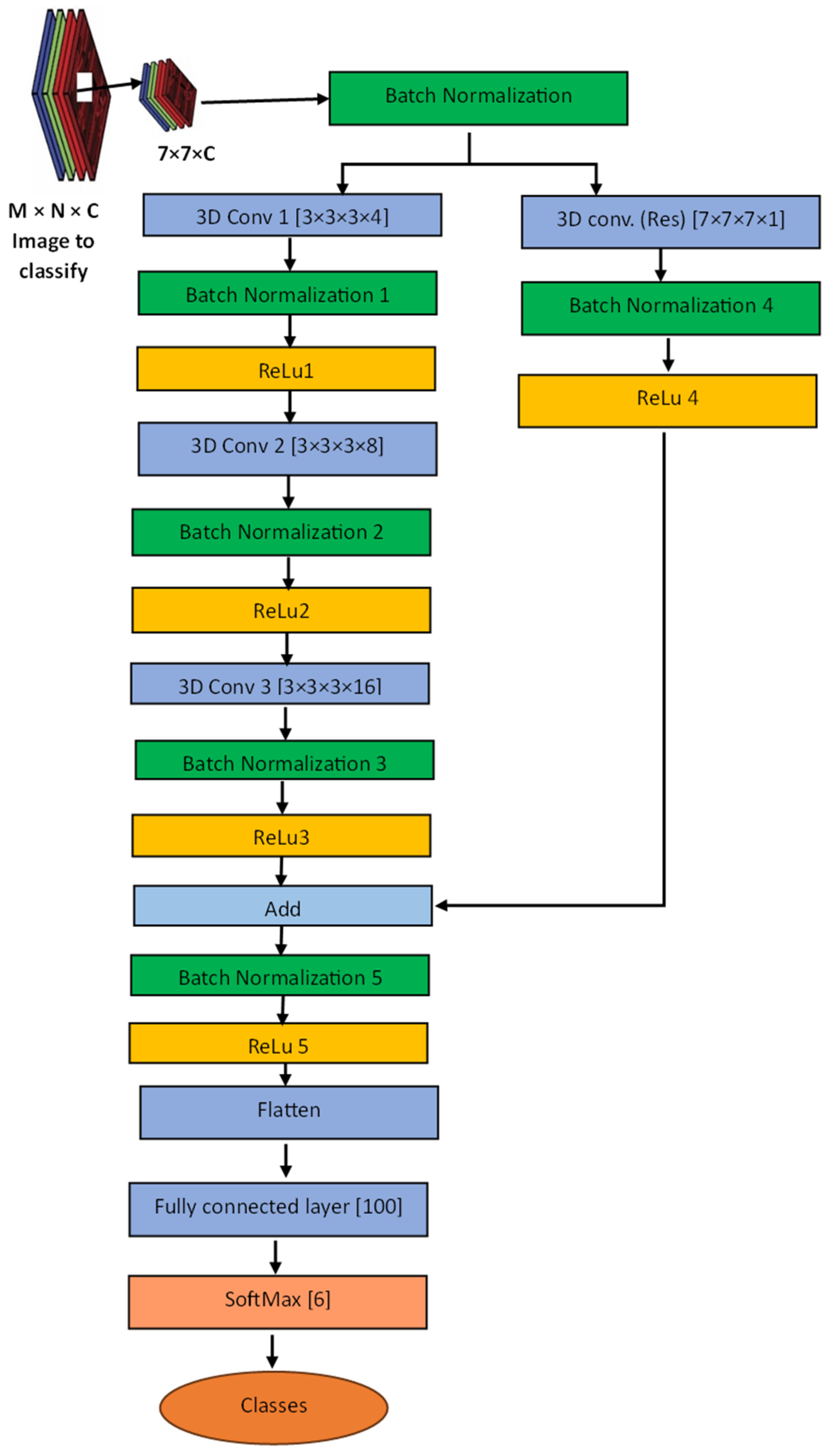
2.2.4. Design of Proposed 3D-CNN Model Architecture

The proposed model is engineered to process a stacked image comprising ASTER image bands, BR images, and selected PC bands as its input. The architectural blueprint of the proposed model is founded on the framework introduced by [17], which refines the design put forth by [18]. The latter incorporates a few 3D convolutional layers, including a residual layer, to enhance the generalization capacity, mitigate overfitting, prevent gradient disappearance, and improve the learning rate. Notably, the proposed model adheres to a consistent use of a small receptive field (3 × 3 × 3) for all convolutional layers, as advocated by [55]; this is particularly effective for spatiotemporal feature extraction, especially in instances where the features possess limited spatial coverage. This uniformity in kernel size across layers is posited to yield more precise results compared with disparate kernel sizes for each layer [56]. The adoption of a small kernel size is necessitated by the modest size of the input patch required, set at 7 × 7 × C, where “C” denotes the number of bands (Figure 2). This configuration allows a 3 × 3 × 3 kernel to perform three convolutions (without maximum pooling, stride, or padding), thereby expediting operations. The choice of the 7 × 7 patch size aims to strike a balance between providing sufficient contextual information and maintaining classification precision, especially considering the 15 m × 15 m resolution of the resampled image and the nature of the deposits under investigation. Additionally, pixels within a small spatial vicinity generally reflect the same underlying material.

The choice of the number of the hidden units used in the convolutional layer is pivotal, as it governs the network’s capacity to learn complex representations by projecting input data into a higher-dimensional space. However, an excessive number of hidden layers may result in learning extraneous patterns, enhancing training accuracy while exerting minimal influence on the model’s testing performance. In light of this, the current model embraces the paradigm of a shallow network with a small patch size, as advocated by [28,57]. The choice of a small patch size is further influenced by the coarse resolution of the ASTER images (30 m). Owing to the shallowness of the architecture, a residual layer is employed to convolve the input image, with its output merged with that of the third convolutional layer before progressing to the fully connected layer. This integration serves to smooth the data, enhance model stability, and augment the generalization capacity of the dense layer [17].

Given that the input image comprises stacked bands with disparate distributions, batch normalization (BN) assumes the role of the initial operation on the input to standardize all input channels to a uniform range. This normalization, computed for each channel (image band), precedes the application of the non-linearization function in the convolutional network. The ratio of filters between subsequent convolutions is set at 1:2, a configuration proven effective in various studies, including those by [28,57]. Consequently, the initial number of filters in the first convolutional layer is stipulated at 4. Finally, a SoftMax classifier is employed after the fully connected layer to categorize outputs into specified classes, with the probability of an input being classified as a particular class [27]. This configuration resulted in a model with only 26,490 parameters. It is noteworthy that out of the total parameters, a total of 26,398 are trainable, rendering the prediction of unclassified pixels within the entire image notably faster. The model predicts the category of the central pixel within a 7 × 7 patch, as the central pixel is considered the most representative of the local context, while the surrounding pixels provide additional context to enhance classification accuracy.

2.2.5. Model Training, Testing, and Evaluation

Following the preparation of training and testing data, 75% of the prepared image patches, centered on each sample location and its surrounding eight pixels, were allocated for training purposes, with the remaining 25% reserved for testing. Within the training dataset, 95% of the samples were further designated for actual training, while 5% were earmarked for validation. The classes were designated numerically from 1 to 6. Class 1 was assigned to iron ore, and classes 2 through 6 corresponded to skarn minerals, intrusions, volcanic wall rocks, vegetation, and glaciers, respectively. The number of training epochs was set at 100 to facilitate a comprehensive examination of model stability.

Upon completion of model training and testing, overall accuracy (OA) and average accuracy (AA) metrics were extracted to assess the model’s efficacy. The OA of each class represents the classification accuracy for that specific class post-model testing. For each class, the overall accuracy of classification is calculated by dividing the number of samples correctly classified by the total number of samples in that class. The overall accuracy for all classes is determined by dividing the sum of samples correctly classified across all classes by the total number of samples tested. The average accuracy denotes the mean of overall accuracy across all classes and is calculated by dividing the overall accuracy for each class by the total number of classes. The values of these accuracy indicators signify how well the model is trained and is capable of distinguishing features it was trained to do.

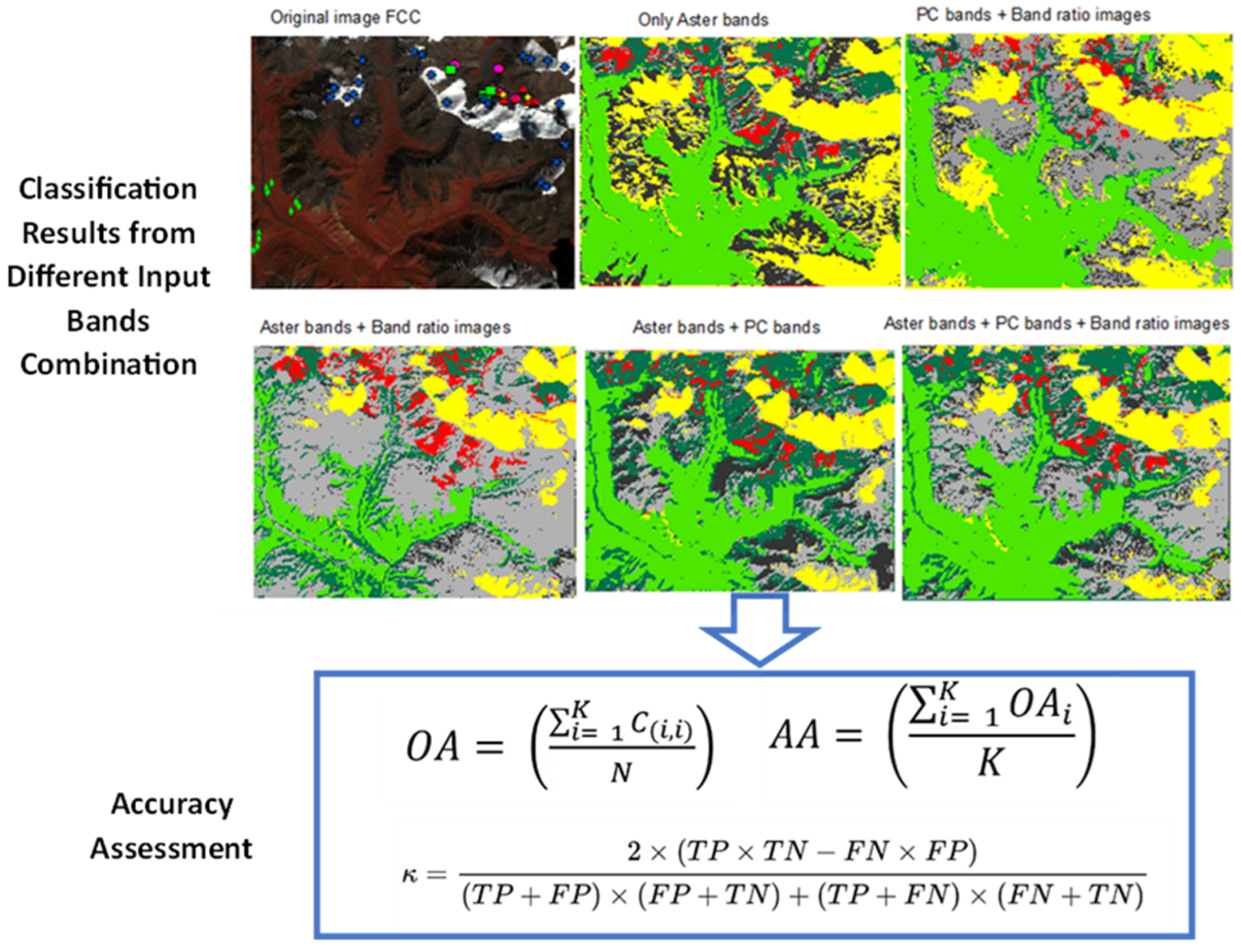
2.2.6. Evaluation of the Impact of BR Images and PC Bands on the Accuracy

The model was specifically configured to operate on a concatenation of multispectral image bands, PC bands, and BR images. To comprehensively gauge the impact of these image derivatives on the accuracy of iron mineral detection and the classification of other minerals, the model underwent additional testing under various configurations: utilizing solely the ASTER image bands, combining ASTER image bands with PC bands, employing ASTER image bands in conjunction with BR images, and utilizing only PC bands and BR images. This systematic evaluation allowed for a nuanced understanding of the contributions of BR images and PC bands to the model’s accuracy. Accuracy indicators such as OA, kappa statistics, and AA were employed to quantify the model’s performance (Figure A5 in Appendix A).

2.2.7. Comparison with Other Methods

To further validate the effectiveness of the proposed approach, we compared the classification results with those from existing methods: (1) a 3D-CNN method proposed by [28], which employs a few 3D convolutional layers (two convolutional layers and a fully connected layer), uses a small image cube size (5 × 5), and has very few parameters while taking full-image spectral bands as inputs; (2) a HybridSN model by [29], consisting of three 3D convolutions, a 2D convolution, and three fully connected layers, using a 25 × 25 image cube size as input, resulting in a large number of parameters; (3) a 3D inception model proposed by [58], which features four branches: the first branch has a 1 × 1 × 1 3D convolutional layer, the second branch has a 3 × 3 × 3 convolutional layer, the third branch includes a 1 × 1 × 1 and a 5 × 5 × 5 convolutional layer, and the fourth branch adds a 3 × 3 × 3 convolutional layer to the general inception architecture; and (4) a 2D-CNN method (AlexNet) proposed by [59], consisting of five convolution layers, three max-pooling layers, two normalization layers, two fully connected layers, and one SoftMax layer. For our data, the AlexNet architecture was modified by reducing the input size to 27 × 27 and omitting the first convolutional and pooling operations. The results were compared in terms of OA, AA, and the kappa coefficient.

2.2.8. Experimental Setting

This study introduces an innovative methodology aimed at enhancing the dimensionality of multispectral satellite image data. The approach integrates relevant band ratios and principal component bands into the existing image bands. Furthermore, it presents a 3D-CNN model characterized by a few convolutional layers, rapid convergence rate, and relatively high accuracy. The proposed model was implemented using Python incorporating the Keras and TensorFlow libraries along with other modules such as “sio”, “os”, and “matplotlib”. This implementation was conducted within a Jupyter Notebook environment, a web-based open-source platform for code development and resource sharing. The “Keras” package provides the building blocks for model configuration and training, while the “sio” and “os” modules are used for handling external files. Data visualization and the generation of prediction maps were achieved using the plotting functionalities of “matplotlib”.

All experiments were conducted on an ASUS Zenbook laptop (ASUS Computer Co., Ltd., Shanghai, China) equipped with an 11th Gen Intel(R) Core (TM) i7-1195G7 processor running at 2.90 GHz and 16 GB of RAM. During model configuration, the parameters were specified as follows: a batch size of 32 patches, a learning rate of 0.001, a dropout rate of 35%, a regularization parameter (L2 parameter) set at 0.001, and kernel and filter sizes in accordance with the specifications outlined in Figure 2. To ensure a thorough assessment of model stability and convergence, the number of training epochs was set at 100. A SoftMax classifier was introduced after the final fully connected layer to classify the outputs into specified classes.

The model’s training, testing, and validation phases were conducted utilizing the prepared image data of the Zhibo deposit. This image comprises 19 bands, encompassing 9 ASTER multispectral bands and 10 bands derived from the original image transformations (4 PC bands and 6 BR images). This image comprises 19 bands, encompassing 9 ASTER multispectral bands and 10 bands derived from the original image transformations (4 principal component bands and 6 band ratio images). The image dimensions are 516 rows by 663 columns, resulting in an image shape of 516 × 663 × 19. The ground truth file was generated by associating the sample points’ coordinates with six distinct classes, encapsulating both environmental and mineral/rock components of interest in the study area. During the ground truth image generation process, sample points were buffered to encompass the immediate adjacent pixels (within 15 m) in all directions. This data augmentation strategy aims to bolster the volume of training pixels available for generating input patches. Importantly, this strategy does not compromise the quality of the training data, as meticulous care was exercised during field sample collection to ensure each sample was acquired in locations where a conspicuous dominance of the target class was apparent within a 30 m proximity.

Subsequent to the data augmentation process, the ground truth image is systematically compiled, and each class is assigned a unique identifier ranging from 0 to 6. The “0” identifier denotes pixels unallocated to any specific class, signifying those to be classified after the training and validation phases.

Table 2. Patches summary.

Class/Patches Category	Class ID	Number of Patches
Iron Ore	1	306
Skarn	2	306
Wall rock	3	126
Intrusion	4	189
Vegetation	5	180
Glacier	6	225
Total	6	1332
Training	-	949
Testing	-	333
Validation	-	50

presents the summary statistics of the total number of pixels for patch preparation for each category, which includes 949 training patches, 50 validation patches, and 333 testing patches. A visual representation of the selected prepared patches for model training, testing, and validation is displayed as a false-color composite in Figure A6 in Appendix A, using ASTER bands 3, 2, and 1 displayed through the red, green, and blue filters, respectively. The four rock components appear visually similar, making them difficult to distinguish with the naked eye, whereas vegetation and glaciers are distinct from the others, allowing for easier classification with minimal error. The evaluation of results was based on the assessment of OA, AA, and the kappa coefficient.

3. Results

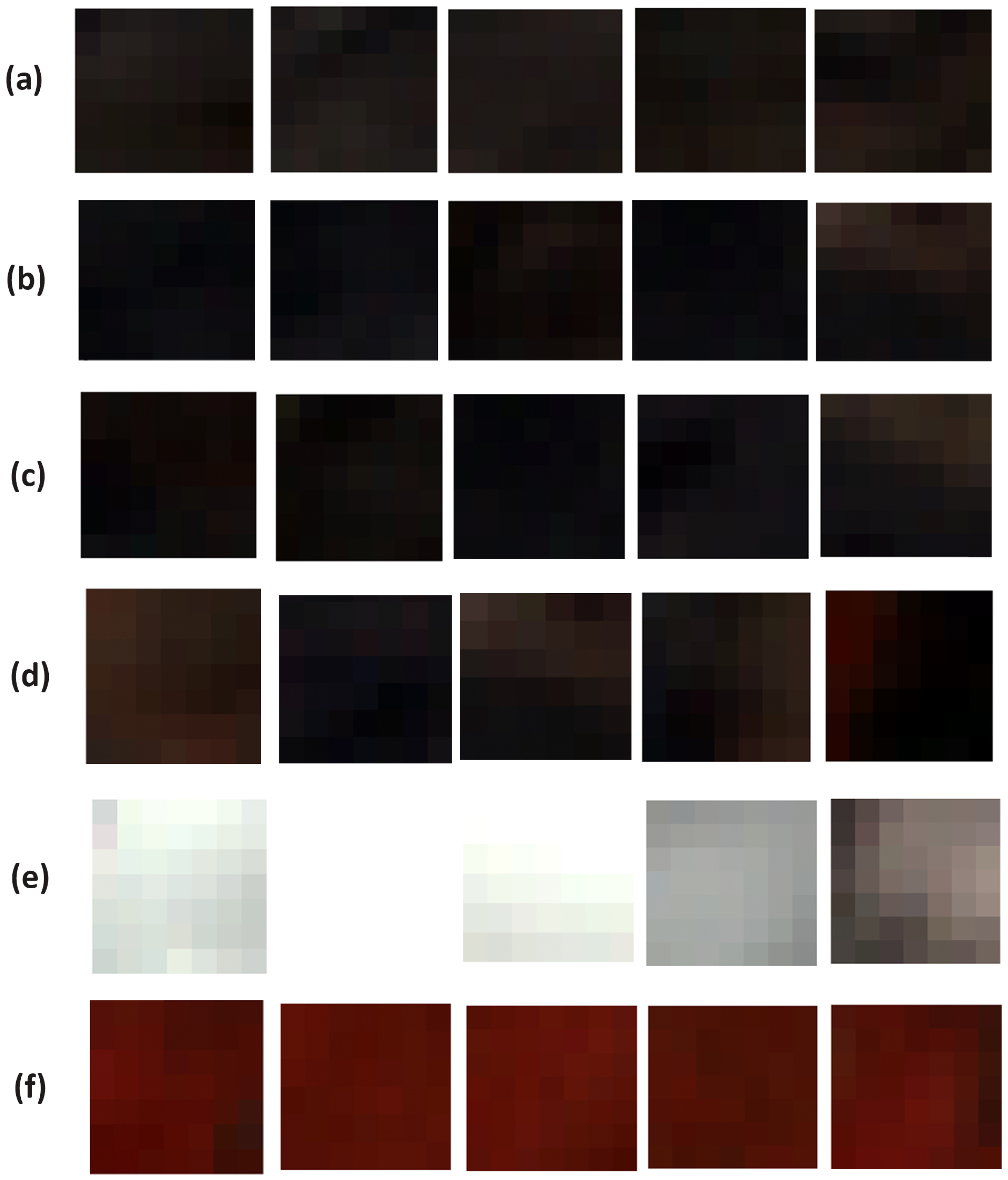
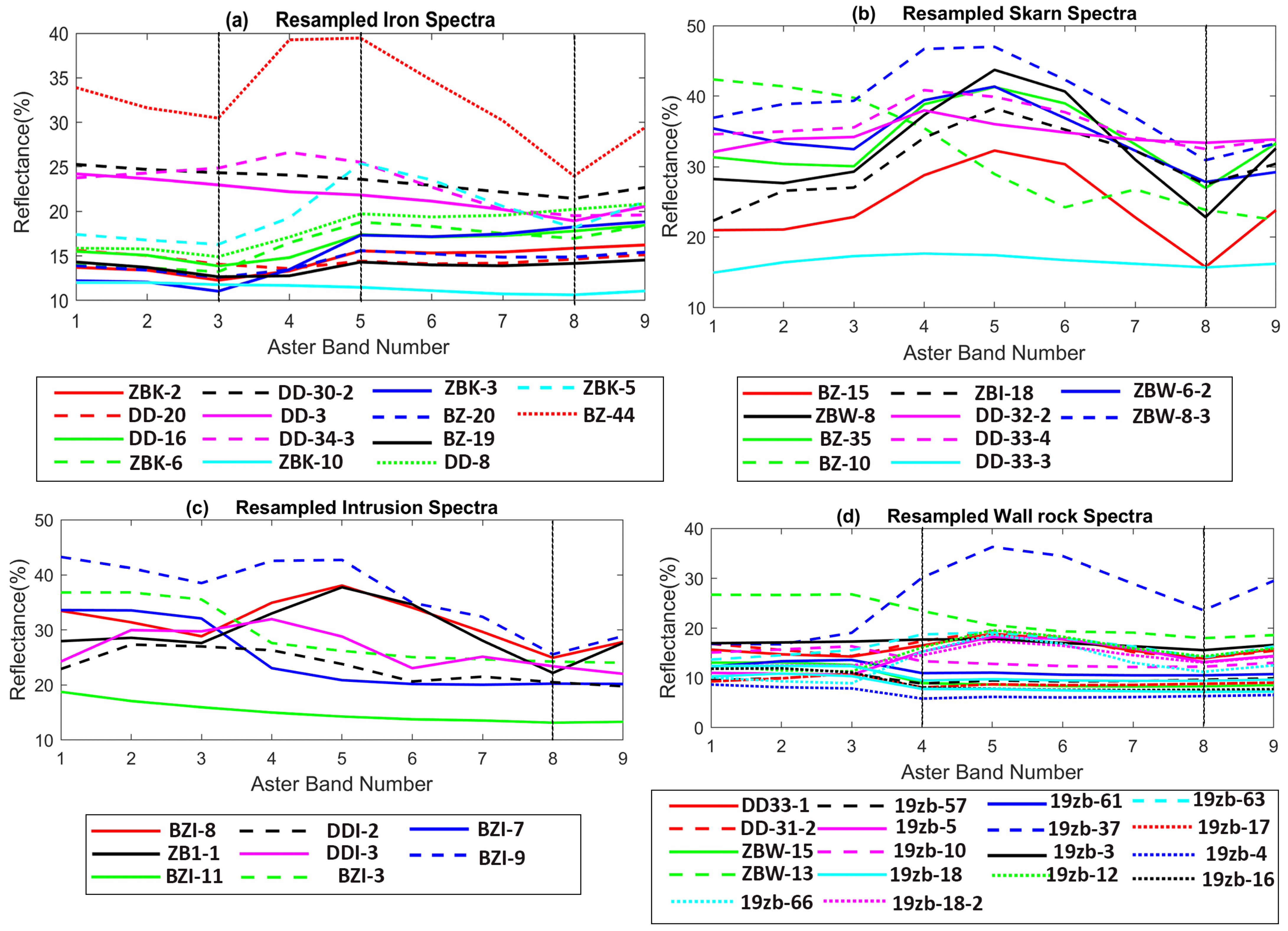
3.1. Processed Samples Spectra

The average ASTER-resampled spectra for some of the selected samples are presented in Figure 3. The resampled spectra of the iron ore exhibit pronounced absorptions within band 3 and band 8, as depicted in Figure 3a. Remarkably, these spectral characteristics bear a striking similarity to the spectra of skarn minerals, featured in Figure 3b. Notably, the spectral profile of iron ore showcases nearly uniform reflectance between bands 5 and 6, while skarn minerals manifest a distinct absorption between these two bands.

Conversely, the spectra of intrusive rock samples exhibit absorption in band 6, in addition to the absorptions observed in band 3, and reflections are present in bands 5 and 7, as noticeable in Figure 3c. This spectral behavior can be attributed to the presence of OH-bearing minerals within the composition of the intrusion rocks [60]. Given that some of the intrusions are identified as granites within the study area, it is notable that granites typically feature absorption features around 2200 nanometers in wavelength (corresponding to ASTER band 7) [61]. Nonetheless, it is noteworthy that specific intrusion samples (BZI-6, 7, and 11) do not display discernible absorption or reflection features across the measured wavelength range (ranging from 400 to 2500 nanometers) for this study. These particular samples exhibit spectral behavior analogous to granodiorite, mirroring the observations in [62].

The spectral plots of the wall rock samples (Figure 3d) exhibit distinguishable spectra between those sourced from Zhibo and Dunde (indicated by sample names beginning with “Z” and “D”, respectively), reflecting the presence of subtly distinct wall rock types in these areas. Specifically, Zhibo deposits predominantly feature andesite, basaltic andesite, and basalt [39], while Dunde deposits comprise basaltic tuff, basaltic crystal tuff, and andesite [44] (Figure 1b,c). This discrepancy in mineral composition contributes to the observed dissimilarities in the spectra. Notably, wall rock spectra from Dunde (DD33-1 and DD-31-2, Figure 3d) closely resemble the spectra of skarn minerals. This resemblance can be attributed to the presence of calcite, epidote, or chlorite in most basaltic tuffs in Dunde (Figure A4 in Appendix A) [63], resulting in a spectral profile featuring a significant absorption around 2330 nm wavelength (ASTER band 8). Coincidentally, these minerals, integral to the basaltic tuff composition, also form part of the skarn minerals in the study deposits [33,63], explaining the observed spectral similarity. Despite this, discrepancies manifest in the VNIR range, where skarn exhibits absorption in band 3, contrasting with the reflection observed in the wall rock (Figure 3b,d).

The spectral profiles of ore samples demonstrate a pattern akin to that of intrusion samples, with a notable distinction in the region between band 6 and band 7, where intrusions exhibit reflection while ores maintain absorption. This divergence in bands 6 and 7 can be attributed to the presence of Al-OH in the mineral composition of both intrusions and ores. The similarities observed suggest common mineral composition as gangue components, owing to the formation of ore minerals between intrusions and wall rocks.

3.2. Selected Band Ratios

The analysis utilized scatter plots of two band ratios per plot (Figure 4) to evaluate their efficacy in differentiating between mineral components. The plot of BR 4/8 against 5/6 (Figure 4a) demonstrated the capability of these ratios to distinguish between ores and skarn minerals, with skarn minerals consistently displaying higher ratio values compared with ores. Additionally, iron ore samples exhibited uniform reflectance between bands 5 and 6, while skarn minerals displayed distinct absorption between these bands.

The scatterplot of BR 2/3 against 4/7 (Figure 4b) indicates that these ratios collectively differentiate between three components, with BR 2/3 greater than 1.023 indicative of iron ore or intrusion rock and inverse values suggesting skarn minerals. Incorporating BR 4/7 provided further discrimination, with intrusions possessing higher BR 4/7 values compared with ore samples. Similarly, BR (8/7)/((2 + 4)/8) effectively separated ores from intrusions (Figure 4c), and BR (2 + 4)/8 proved valuable in resolving classification confusion between ores and wall rocks (Figure 4d), although it could not separate wall rocks from the other classes. However, BR (6 + 9)/(7 + 8) exhibited limited capability in distinguishing any one component from the others despite slight spectral pattern variations within the ratio across different classes. BR (5/3 + 1/2) and BR 2/1 displayed heightened sensitivity, making component differentiation challenging. Other tested band ratios encountered difficulties in isolating skarn samples, possibly due to the presence of calcite and chlorite in the skarn minerals across the study areas. Additionally, band ratios such as BR (2 + 4)/3 and (2/3)/((2 + 4)/8), aimed at enhancing iron content and differentiating iron ores from other components, showed no apparent clustering for the same samples.

Table 3. Summary of the selected BRs.

BR	Ore	Skarn	Intrusions	Wall Rock	Remark
5/6	√	√			Differentiate iron ores from skarns
4/8	√	√			Separate iron ore from skarn
2/3	√	√	√		Separate skarn from iron ore and intrusion
(8/7)/ ((2 + 4)/8)	√		√		Separate iron ore from intrusions
4/7	√		√		Separate iron ore from intrusions
(2 + 4)/8	√	√	√	√	Separate iron ore from other components

provides the summary list of the selected BRs.

3.3. Selected Principal Components Bands

The selection of the requisite PCs adheres to a concept widely adopted in various research works, including those by [18,27]. This concept involves identifying PC bands whose eigenvectors possess the highest opposing sign values corresponding to the major absorption and reflection bands of the targeted component, thereby characterizing that component. The eigenvectors matrix, detailed in

Table 4. The eigenvector matrix from the PCA of the nine ASTER bands (VNIR and SWIR).

Eigenvectors	Band 1	Band 2	Band 3	Band 4	Band 5	Band 6	Band 7	Band 8	Band 9
PC 1	0.5547	0.5725	0.5841	0.0745	0.0604	0.0683	0.0695	0.0517	0.0453
PC 2	0.2119	−0.1415	0.0899	−0.5397	−0.3950	−0.3922	−0.3413	−0.3253	−0.3219
PC 3	−0.3287	−0.3098	0.6716	0.3413	−0.2152	−0.1120	−0.1800	−0.2223	−0.2963
PC 4	0.3354	−0.0532	0.3906	0.5891	0.1568	0.1203	−0.1589	−0.4132	−0.3873
PC 5	−0.0426	−0.2432	0.2046	0.4391	−0.6036	−0.3817	0.1846	0.4002	0.0052
PC 6	−0.6003	−0.6672	0.0657	0.0588	0.0917	0.1051	−0.3529	−0.1676	0.1207
PC 7	0.1629	−0.1326	0.0257	0.0261	−0.5661	0.6326	−0.3416	−0.0412	0.3400
PC 8	−0.1877	−0.1725	0.0155	−0.2053	−0.2049	0.4981	0.4797	0.0451	−0.6086
PC 9	−0.0540	0.0422	0.0015	0.0227	−0.1852	−0.0978	0.5619	−0.6924	0.3948

PC 3–5, and 7 are selected due to the opposite contributions observed from the bands corresponding to the reflection and absorption of the targeted minerals.

, reveals that PC 3 exhibits moderate negative contributions in bands 2 and 1 (−0.32 and −0.31, respectively), coupled with a strong positive contribution in band 3 (0.67), which aligns with the reflection and major absorption bands within the spectra of the iron ore samples. Consequently, PC 3 is deemed a suitable selection for inclusion in the final set of image bands to be employed as input into the model, as it appears to contain vital information conducive to the simple detection of iron minerals.

Likewise, PC 4 demonstrates a moderate negative contribution in band 8 (−0.41) and a positive contribution in band 4 (0.59) (as outlined in Table 4), aligning with the absorption and reflection bands shared by the skarn and iron ore spectra. This characteristic makes PC 4 potentially useful for enhancing iron oxides, as previously proposed by [13]. PC 5, on the other hand, exhibits a positive contribution in band 4 (0.44) along with a negative contribution in band 5 (−0.60). This nuanced behavior corresponds to the spectral signature of volcanic wall rocks, which uniquely display absorption in band 4 followed by reflection in band 5, distinguishing them from other components, which generally exhibit reflection in both bands. Notably, PC band 7 displays its highest positive contribution from band 6 (0.63) and the most significant negative contribution from band 5 (−0.57), indicating the spectral characteristics of skarn samples within the study area, where band 5 serves as an absorption shoulder band, while band 6 functions as the primary absorption band.

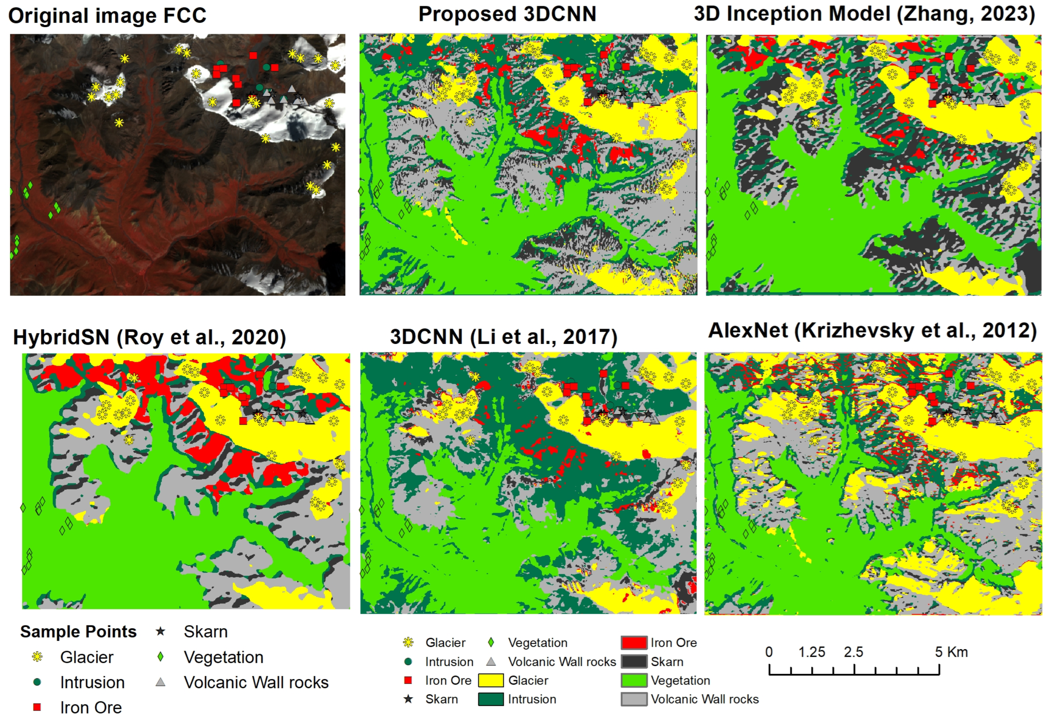
3.4. Mineral Detection Using the Proposed Model

In this study, we applied a novel model for the detection and classification of minerals within the Zhibo deposit. The methodology involved a comprehensive approach encompassing training, testing, and validation phases on stacked images of the deposit. The model was optimized using the “Adam” optimizer, with “categorical cross-entropy” serving as the loss function and “accuracy” as the evaluation metric. A best model was selected for subsequent classification and prediction tasks, culminating in the production of a classified image, as illustrated in Figure 5 (top center).

The classified image revealed the predominant presence of iron minerals in the northwestern region of the deposit, extending toward the southeast, particularly concentrated at the contact zone between the intrusion and wall rocks. This observation aligns with previous geological reports on the spatial distribution pattern of ore minerals within the deposit [39]. Individual class classification results demonstrated noteworthy accuracy rates, particularly with 100% accuracy achieved for iron ores, intrusions, vegetation, and glaciers. Skarn minerals and wall rocks exhibited accuracies of 84.62% and 95.24%, respectively (

Table 5. Comparison of the proposed method with the existing methods.

	Accuracy (%)
Method	Iron Ore	Skarn	Intrusion	Wall Rock	Vegetation	Glacier	OA	AA	Kappa
Proposed model	100	84.62	100	95.24	100	100	96.95	94.87	95.93
HybridSN	100	100	92.86	85.71	100	100	97.01	94.93	96.21
3D-CNN	75.00	76.92	92.86	42.86	100	100	87.78	81.27	82.78
3D Inception Model	100	92.31	100	95.24	100	98.08	95.92	93.60	94.44
AlexNet	100	61.54	100	85.71	100	100	93.89	91.21	91.87

). The training phase lasted approximately 121.22 s, with subsequent prediction and testing phases completed efficiently within 0.828 s, indicating robust convergence of the model.

The classification result analysis reveals that the proposed methodology demonstrates commendable performance metrics. The OA stands at 96.95%, with an AA of 94.87% and a kappa coefficient of 95.93%. Notably, these results exhibit an improvement in the OA, AA, and kappa coefficient of 1.03, 1.27, and 1.49, respectively, in comparison with outcomes attained utilizing the 3D inception model introduced by [58] (Table 5). This disparity underscores a significant achievement of the proposed model despite its linear architectural design relative to the more complex parallel architecture of the 3D inception network. Relative to a 3D-CNN model proposed by [28], which shares a similarly shallow architectural design, the proposed model exhibits significant improvements of 9.17, 13.6, and 13.15 in OA, AA, and kappa coefficient accuracy, respectively. The disparity underscores the efficacy of the proposed model, raising inquiries into its underlying mechanisms. In contrast with the 2D-CNN model, our proposed model demonstrates improvements of 3.06%, 3.66%, and 4.06% in OA, AA, and kappa coefficient accuracy, respectively. Notably, the 2D-CNN model surpasses the 3D-CNN model proposed by [28], potentially due to the latter’s comparatively shallow network architecture, as highlighted in [28]. Comparatively, against the HybridSN model [29], the proposed model exhibits a marginal shortfall of less than 0.06 in both OA and AA, despite possessing significantly fewer parameters and a less complex architectural design (Table 5).

In summary, the proposed methodology and model demonstrate exceptional performance in identifying and detecting skarn iron minerals within the Zhibo deposit, surpassing existing methodologies in accuracy while maintaining a simpler and more efficient architecture.

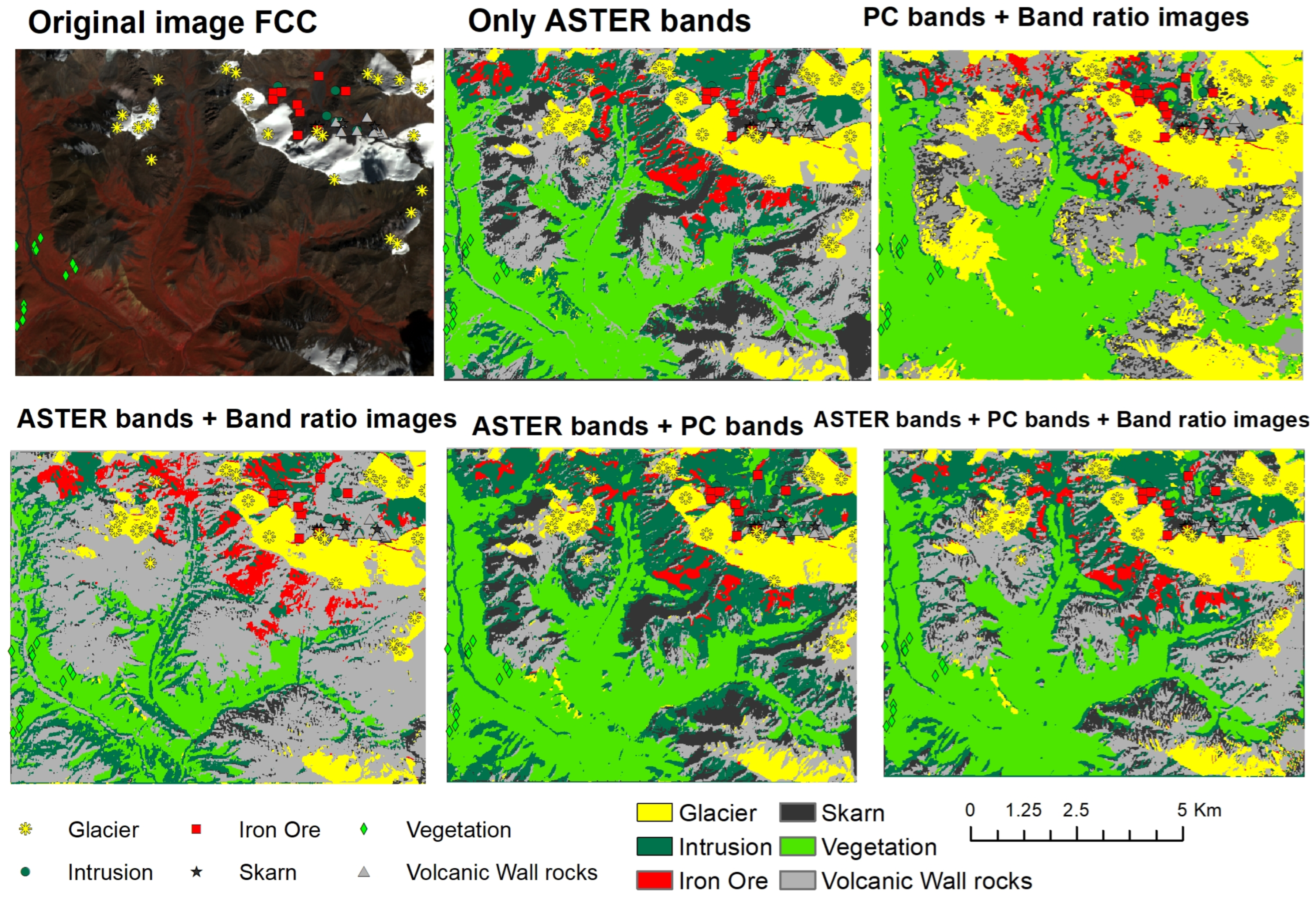
3.5. Evaluation of the Impact of the BR Images and PC Bands

The strategic integration of band ratios and principal component bands alongside the original ASTER image bands was undertaken not only to augment the number of bands/channels within the input image but also to capitalize on the unique strengths of these derivatives in enhancing discernible features. Therefore, the evaluation sought to scrutinize the effects of incorporating BR images and PC bands into the original ASTER image bands on mineral classification accuracy.

The results (Figure 6 and

Table 6. Accuracy assessment results from five different input configurations.

	Accuracy (%)
Image Used	Iron Ore	Skarn	Intrusion	Wall Rock	Vegetation	Glacier	OA (%)	AA (%)	K (%)
Only ASTER bands	100	84.62	92.86	76.19	100	98.08	93.13	91.96	90.91
PCs + BR	100	53.85	64.29	76.19	100	96.15	87.78	82.39	83.81
ASTER bands + BR	100	15.38	64.29	95.24	100	100	87.02	79.15	82.60
ASTER bands + PCs	100	76.92	100	85.71	100	98.08	94.65	92.93	93.45
ASTER bands + PCs + BR	100	84.62	100	95.24	100	100	96.95	94.87	95.93

The proposed band combination has retained the best classification results for each of the classes.

) indicated that the inclusion of selectively chosen band ratios alongside the original ASTER bands yielded an overall classification accuracy of 87.02%, with an average classification accuracy of 79.15% across all classes. While band ratios improved the classification of ores and volcanic wall rocks, they introduced significant confusion in differentiating skarn from intrusions and wall rocks, resulting in misclassification rates exceeding 80% for skarns and approximately 35% for intrusions.

Remarkably, utilizing solely ASTER bands as the input parameters yielded significantly higher accuracy rates (OA = 93.13%, AA = 91.96%, and kappa = 90.91%) compared with scenarios involving the incorporation of ASTER bands with band ratios or PC bands with band ratios. The amalgamation of ASTER bands with selected PC bands yielded a slightly improved result, with an OA of 94.65%, AA of 93.45%, and kappa coefficient of 92.93%. However, this enhancement posed challenges in accurately classifying wall rocks, as some were misclassified as skarn or intrusions. Nevertheless, the inclusion of PC bands made a constructive contribution to both the overall and average classification accuracies.

The classified image derived from the combination of ASTER bands, PC bands, and band ratios (Figure 6) presented more visually appealing and statistically more accurate results when compared with the four alternative band combinations explored in this study, as summarized in Table 6. This particular combination notably amended the misclassification of intrusions evident in both the northern and central regions of the classified image when ASTER bands were used in conjunction with PC bands. Additionally, it addressed the misclassification of skarns observed in both the western and southeastern portions of the same image. This band combination further improved the classification accuracy beyond what was observed when exclusively employing ASTER bands in conjunction with PC bands. Specifically, the OA increased from 94.65% to 96.95%, reflecting a 2.3% improvement, while the average accuracy rose from 93.45% to 94.87%, indicating a 1.42% enhancement.

4. Discussion

4.1. Spectral Analysis and Data Selection

Spectral analysis unveiled distinct absorption and reflection patterns among the different mineral components. The majority of samples in each class exhibited absorption in band 8, likely due to the presence of calcite as a gangue mineral in the iron ore samples, part of the skarn mineral composition, or a constituent of the basaltic tuff in the wall rocks. This absorption, observed around 2330 nanometers, may be induced by the vibrational effect generated by the C-O bond in calcite [61] or the Fe-OH bonding [48]. Similarities between the spectra of the iron ore and skarn minerals (Figure 3a,b) suggest the presence of iron minerals in the majority of the skarn samples, which efficiently absorb radiation within the wavelength range of 500 to 1000 nanometers [50,64], particularly in the near-infrared region spanning 780 to 860 nanometers corresponding to ASTER band 3. These observed similarities and differences in electromagnetic radiation absorptions and reflections across the nine ASTER bands among the various minerals and rock components underscore the importance of band selection and derivation of ratios for accurate mineral identification and characterization.

The scatter plots of the band ratios (Figure 4) illustrate the efficacy of different ratios in distinguishing between mineral components with specific ratios, such as BR 4/8 and BR 2/3, showing consistent patterns in differentiating ores from skarn minerals. Similarly, the scatterplot of BR 5/6 against 4/8 convincingly highlights the ability of these two band ratios to distinguish ores from skarn minerals, with skarn minerals exhibiting higher ratio values in both ratios compared with ores (Figure 4a). BR (5/3 + 1/2) and BR 2/1, specifically identified by [48] for ferrous and ferric iron enhancement, could not perform this task efficiently. Notably, these ratios exhibited no distinct boundary between components. This may be attributed to the small and insignificant weight percentage of Fe in the skarn samples from all the sites.

The PCs, derived from PCA, constitute a significant aspect of this research’s consideration. These bands are deemed valuable due to their potential to mitigate data redundancy, enhance classification accuracy, and simultaneously reduce processing time, as documented in studies such as [27,54]. Nevertheless, it is imperative to acknowledge that certain PCs, particularly those associated with higher PC bands, may contain minimal information and exhibit very low variance, appearing similar to noise, as noted by [65]. To optimize the model’s performance, PCs 3, 4, 5, and 7 emerge as the only PCs among the nine computed PCs that contain pertinent information corresponding to the four components (iron ores, skarn, intrusion, and volcanic wall rocks) of interest in this research and are selected for inclusion in the image bands fusion.

4.2. Methods Comparison

During mineral detection, high accuracy was observed in iron ore classification, attributed to the complementary support provided by the multiple band ratio images integrated into the input data. However, relatively lower accuracy in distinguishing wall rocks from skarn minerals may be due to the presence of calcite and chlorite, significant constituents of both classes, particularly in the basaltic tuffs prevalent in the Zhibo deposit [39]. These mineral compositions posed challenges for the model, particularly when using broader wavelength range images like the ASTER image utilized in this study.

Relative to other models evaluated, the proposed model exhibited superiority, emphasizing that the depth of a network does not always correlate with superior performance, as deeper networks may capture extraneous patterns that may augment training accuracy but offer marginal benefits to testing performance [57]. The integration of residual layers within the proposed model architecture was identified as a key contributor to its superiority, enhancing generalization capacity, improving model stability, and mitigating overfitting, thereby preventing issues such as gradient disappearance and augmenting the learning rate [17,18,66]. Additionally, the utilization of larger patches in the other methods (HybridSN, AlexNet, and the 3D inception model) leads to overgeneralization in classification outcomes, resulting in smoother images that prevent subtle spatial variations typical of skarn iron formations, characterized by the sharp contact zonation between ores and surrounding rocks [38,67,68].

The close correspondence between the results from the proposed model and the HybridSN model underscores the pivotal role of PC bands in enhancing image classification accuracy. However, the proposed method demonstrated superior performance in identifying intrusive and wall rocks, with accuracies of 100% and 95.24%, respectively, compared with 92.86% and 85.71%, respectively, achieved by the HybridSN method (Table 5). This superiority may be attributed to the inclusion of band ratio images in the proposed model’s input configuration, which aids in reducing confusion between wall rocks and iron ore or skarn minerals and enhances the spectral response of intrusions. Nonetheless, the HybridSN method exhibits slightly superior accuracy in skarn mineral classification.

4.3. Impact of Band Integration on Classification Accuracy

During the evaluation of the impact of the integration of PCs, band ratio images, and original ASTER bands, the incorporation of BRs into the ASTER bands notably influenced the classification outcomes, reducing misclassified pixels in the context of glaciers and wall rocks and thereby enhancing the accuracy of the classified image, particularly in glaciers and wall rock categorization. However, the remarkable results obtained while using only ASTER bands as input relative to the use of either ASTER bands with band ratios or PC bands with band ratios was unexpected, considering the anticipated favorable contribution of band ratios to accuracy, given their documented potential to enhance the spectral signatures of targeted features in prior studies [3,13,51,52,53]. Additionally, the classified image resulting from the integration of PC bands with ASTER bands exhibited notable visual and statistical improvements in mitigating misclassifications observed in the classified image derived from ASTER bands in conjunction with band ratios (Figure 6). However, this integration led to a reduction in the accuracy of wall rock classification, with some wall rocks erroneously classified as skarn or intrusions. Consequently, the pursuit of a solution through the simultaneous incorporation of all three sets of bands was prompted.

The results from the combination of all three sets of bands consistently retained the highest classification accuracy among the various combinations explored, underscoring the importance of considering the diversity of input channels in enhancing classification accuracy. Further investigation is warranted to understand the specific mechanisms driving this enhancement. However, the most plausible explanation for this enhancement could be attributed to the notion that the accuracy of the 3D-CNN model escalates in tandem with an increase in diversity afforded by a higher number of channels in the input layer. This expansion enables the capture of interdependencies and relationships between the various bands or channels, as posited by [69]. Notably, combinations featuring only PC bands showed reduced accuracy in classifying wall rocks and glaciers compared with combinations featuring only band ratios. This positive impact of different band combinations on classification outcomes underscores the importance of considering the diversity of input channels in enhancing classification accuracy.

5. Conclusions

This study introduces a novel 3D-CNN model architecture that incorporates the strategic integration of band ratios and principal component bands alongside the original ASTER image bands to enhance mineral detection accuracy. The proposed model architecture presents a streamlined, efficient, and effective framework distinguished by a notable reduction in parameters compared with prevailing models in the field. The incorporation of image derivatives notably improves classification accuracy and expedites model predictions. The fusion of image bands demonstrates synergistic advantages, resulting in the highest observed overall and average accuracy when compared with the alternative combinations of bands evaluated. Specifically, ASTER bands are found to play a pivotal role in optimizing accuracy for skarn classification, while principal component bands notably enhance intrusion classification accuracy. Additionally, band ratio images significantly contribute to the accuracy of wall rock classification. Each composite input image configuration achieves maximal accuracy for iron ore classification. Remarkably, the model exhibits versatility in handling both high- and low-spectral-resolution images without necessitating adjustments to kernel sizes. These findings underscore the importance of considering the diversity of input channels in neural network models to enhance mineral detection accuracy, warranting further investigation into the specific mechanisms underlying this enhancement.

References

1. Galdames, F.J.; Perez, C.A.; Estévez, P.A.; Adams, M. Rock lithological classification by hyperspectral, range 3D and color images. Chemom. Intell. Lab. Syst. 2019, 189, 138–148. [Google Scholar] [CrossRef]
2. Huang, S.; Chen, S.B.; Zhang, Y.Z. Comparison of altered mineral information extracted from ETM+, ASTER and Hyperion data in Águas Claras iron ore, Brazil. IET Image Process. 2019, 13, 355–364. [Google Scholar] [CrossRef]
3. Son, Y.S.; Lee, G.; Lee, B.H.; Kim, N.; Koh, S.M.; Kim, K.E.; Cho, S.J. Application of ASTER Data for Differentiating Carbonate Minerals and Evaluating MgO Content of Magnesite in the Jiao-Liao-Ji Belt, North China Craton. Remote Sens. 2022, 14, 181. [Google Scholar] [CrossRef]
4. Rajendran, S.; Nasir, S. Mapping of Moho and Moho Transition Zone (MTZ) in Samail ophiolites of Sultanate of Oman using remote sensing technique. Tectonophysics 2015, 657, 63–80. [Google Scholar] [CrossRef]
5. Abdeen, M.; Thurmond, A.K.; Abdelsalam, M.; Stern, B. Use of TERRA ASTER band-ratio images for geological mapping in arid regions: The Neo-Proterozoic Allaqi suture, Egypt. Egypt J. Remote Sens. Space Sci. 2002, 5, 19–40. [Google Scholar]
6. Amer, R.; Kusky, T.; Ghulam, A. Lithological mapping in the Central Eastern Desert of Egypt using ASTER data. J. Afr. Earth Sci. 2010, 56, 75–82. [Google Scholar] [CrossRef]
7. Gad, S.; Kusky, T. ASTER spectral ratioing for lithological mapping in the Arabian-Nubian shield, the Neoproterozoic Wadi Kid area, Sinai, Egypt. Gondwana Res. 2007, 11, 326–335. [Google Scholar] [CrossRef]
8. Ninomiya, Y. A Stabilized Vegetation Index and Several Mineralogic Indices Defined for ASTER VNIR and SWIR Data. IEEE Int. Geosci. Remote Sens. Symp. IGARSS’03 2003, 3, 1552–1554. [Google Scholar]
9. Crósta, A.P.; Filho, C.R.D.S. Searching for gold with ASTER. Earth Obs. Mag. 2003, 12, 38–41. [Google Scholar]
10. Zhang, X.; Pazner, M.; Duke, N. Lithologic and mineral information extraction for gold exploration using ASTER data in the south Chocolate Mountains (California). ISPRS J. Photogramm. Remote Sens. 2007, 62, 271–282. [Google Scholar] [CrossRef]
11. Hecker, C.; Van Der Meijde, M.; Van Der Werff, H.; Van Der Meer, F.D. Assessing the influence of reference spectra on synthetic SAM classification results. IEEE Trans. Geosci. Remote Sens. 2008, 46, 4162–4172. [Google Scholar] [CrossRef]
12. Kruse, F.A.; Boardman, J.W.; Huntington, J.F. Comparison of airborne hyperspectral data and EO-1 Hyperion for mineral mapping. IEEE Trans. Geosci. Remote Sens. 2003, 41, 1388–1400. [Google Scholar] [CrossRef]
13. Gabr, S.; Ghulam, A.; Kusky, T. Detecting areas of high-potential gold mineralization using ASTER data. Ore Geol. Rev. 2010, 38, 59–69. [Google Scholar] [CrossRef]
14. Magendran, T.; Sanjeevi, S. Hyperion image analysis and linear spectral unmixing to evaluate the grades of iron ores in parts of Noamundi, Eastern India. Int. J. Appl. Earth Obs. Geoinf. 2014, 26, 413–426. [Google Scholar] [CrossRef]
15. Chang, C.I.; Wang, S. Constrained band selection for hyperspectral imagery. IEEE Trans. Geosci. Remote Sens. 2006, 44, 1575–1585. [Google Scholar] [CrossRef]
16. Xiao, D.; Le, B.T.; Ha, T.T.L. Iron ore identification method using reflectance spectrometer and a deep neural network framework. Spectrochim. Acta A Mol. Biomol. Spectrosc. 2021, 248, 119168. [Google Scholar] [CrossRef]
17. Xiao, D.; Vu, Q.H.; Le, B.T.; Ha, T.T.L. A method for mapping and monitoring of iron ore stopes based on hyperspectral remote sensing-ground data and a 3D deep neural network. Neural. Comput. Appl. 2023, 35, 12221–12232. [Google Scholar] [CrossRef]
18. Zhao, Y.; Wu, P.; Wang, J.; Li, H.; Navab, N.; Yakushev, I.; Weber, W.; Schwaiger, M.; Huang, S.C.; Cumming, P.; et al. A 3D Deep Residual Convolutional Neural Network for Differential Diagnosis of Parkinsonian Syndromes on 18F-FDG PET Images. In Proceedings of the 2019 41st Annual International Conference of the IEEE Engineering in Medicine and Biology Society (EMBC), Berlin, Germany, 23 July 2019; pp. 3531–3534. [Google Scholar]
19. Tomita, N.; Jiang, S.; Maeder, M.E.; Hassanpour, S. Automatic post-stroke lesion segmentation on MR images using 3D residual convolutional neural network. Neuroimage Clin. 2020, 27, 102276. [Google Scholar] [CrossRef]
20. Sabins, F.F., Jr. Remote Sensing: Principles and Interpretation, 2nd ed.; WH Freeman & Company: New York, NY, USA, 1987. [Google Scholar]
21. Ghoneim, S.M.; Salem, S.M.; El-Wahid, K.H.A.; Anwar, M.; Hegab, M.A.E.-R.; Soliman, N.M.; Ali, H.F. Application of remote sensing techniques to identify iron ore deposits in the Central Eastern Desert, Egypt: A case study at Wadi Karim and Gabal El-Hadid areas. Arab. J. Geosci. 2022, 15, 1596. [Google Scholar] [CrossRef]
22. Cardoso-Fernandes, J.; Teodoro, A.C.; Lima, A. Remote sensing data in lithium (Li) exploration: A new approach for the detection of Li-bearing pegmatites. Int. J. Appl. Earth Obs. Geoinf. 2019, 76, 10–25. [Google Scholar] [CrossRef]
23. Ahmadi, H.; Uygucgil, H. Targeting iron prospective within the Kabul Block (SE Afghanistan) via hydrothermal alteration mapping using remote sensing techniques. Arab. J. Geosci. 2021, 14, 183. [Google Scholar] [CrossRef]
24. Jolliffe, I.T. Principal Component Analysis; Springer: New York, NY, USA, 2002. [Google Scholar]
25. Abdi, H.; Williams, L.J. Principal component analysis. Wiley Interdiscip. Rev. Comput. Stat. 2010, 2, 433–459. [Google Scholar] [CrossRef]
26. Jackson, J.E. A User’s Guide to Principal Components; John Wiley & Sons: Hoboken, NJ, USA, 2005. [Google Scholar]
27. Yue, J.; Zhao, W.; Mao, S.; Liu, H. Spectral-spatial classification of hyperspectral images using deep convolutional neural networks. Remote Sens. Lett. 2015, 6, 468–477. [Google Scholar] [CrossRef]
28. Li, Y.; Zhang, H.; Shen, Q. Spectral-spatial classification of hyperspectral imagery with 3D convolutional neural network. Remote Sens. 2017, 9, 67. [Google Scholar] [CrossRef]
29. Roy, S.K.; Krishna, G.; Dubey, S.R.; Chaudhuri, B.B. HybridSN: Exploring 3-D-2-D CNN Feature Hierarchy for Hyperspectral Image Classification. IEEE Geosci. Remote Sens. Lett. 2020, 17, 277–281. [Google Scholar] [CrossRef]
30. Hu, Y.; Tian, S.; Ge, J. Hybrid Convolutional Network Combining Multiscale 3D Depthwise Separable Convolution and CBAM Residual Dilated Convolution for Hyperspectral Image Classification. Remote Sens. 2023, 15, 4796. [Google Scholar] [CrossRef]
31. Gopinathan, P.; Priyadarsi, R.; Subramani, T.; Karunanidhi, D. Detection of iron-bearing mineral assemblages in Nainarmalai granulite region, south India, based on satellite image processing and geochemical anomalies. Environ. Monit. Assess. 2022, 194, 866. [Google Scholar]
32. Hou, T.; Zhang, Z.; Pirajno, F.; Santosh, M.; Encarnacion, J.; Liu, J.; Zhao, Z.; Zhang, L. Geology, tectonic settings and iron ore metallogenesis associated with submarine volcanism in China: An overview. Ore Geol. Rev. 2014, 57, 498–517. [Google Scholar] [CrossRef]
33. Zhang, Z.; Hong, W.; Jiang, Z.; Duan, S.; Xu, L.; Li, F.; Guo, X.; Zhao, Z. Geological Characteristics and Zircon U-Pb Dating of Volcanic Rocks from the Beizhan Iron Deposit in Western Tianshan Mountains, Xinjiang, NW China. Acta Geol. Sin.-Engl. Ed. 2012, 86, 737–747. [Google Scholar] [CrossRef]
34. Zhu, Y.; Zhou, J.; Song, B.; Zhang, L.; Guo, X. Age of the Dahalajunshan Formation in Xinjiang and its disintegration. Geol. China 2006, 33, 487–497. [Google Scholar]
35. Jiang, Z.; Zhang, Z.; Wang, Z.; Duan, S.; Li, F.; Tian, J. Geology, geochemistry, and geochronology of the Zhibo iron deposit in the Western Tianshan, NW China: Constraints on metallogenesis and tectonic setting. Ore Geol. Rev. 2014, 57, 406–424. [Google Scholar] [CrossRef]
36. Feng, W.; Zhu, Y. Petrogenesis and tectonic implications of the late Carboniferous calc-alkaline and shoshonitic magmatic rocks in the Awulale mountain, western Tianshan. Gondwana Res. 2019, 76, 44–61. [Google Scholar] [CrossRef]
37. Wang, X.S.; Zhang, X.; Gao, J.; Li, J.L.; Jiang, T.; Xue, S.C. A slab break-off model for the submarine volcanic-hosted iron mineralization in the Chinese Western Tianshan: Insights from Paleozoic subduction-related to post-collisional magmatism. Ore Geol. Rev. 2018, 92, 144–160. [Google Scholar] [CrossRef]
38. Li, H.-M.; Li, L.-X.; Yang, X.-Q.; Cheng, Y.-B. Types and geological characteristics of iron deposits in China. J. Asian Earth Sci. 2015, 103, 2–22. [Google Scholar] [CrossRef]
39. Luo, W.; Zhang, Z.; Duan, S.; Jiang, Z.; Wang, D.; Chen, J.; Sun, J. Geochemistry of the Zhibo submarine intermediate-mafic volcanic rocks and associated iron ores, Western Tianshan, Northwest China: Implications for ore genesis. Geol. J. 2018, 53, 3147–3172. [Google Scholar] [CrossRef]
40. Zhang, Z.; Li, H.; Li, J.; Song, X.Y.; Hu, H.; Li, L.; Chai, F.; Hou, T.; Xu, D. Geological settings and metallogenesis of high-grade iron deposits in China. Sci. China Earth Sci. 2021, 64, 691–715. [Google Scholar] [CrossRef]
41. Ping, S.; HongDi, P.; ChangHao, L.; HaoXuan, F.; Yang, W.; FuPin, S.; XinCheng, G.; WenGuang, L. Carboniferous ore-controlling volcanic apparatus and metallogenic models for the large-scale iron deposits in the Western Tianshan, Xinjiang. Acta Petrol. Sin. 2020, 36, 2845–2868. [Google Scholar] [CrossRef]
42. Li, C.; Shen, P.; Zhang, X.; Shi, F.; Feng, H.; Pan, H.; Wu, Y.; Li, W. Mineralogy and mineral chemistry related to the Au mineralization in the Dunde Fe-Zn deposit, western Tianshan. Ore Geol. Rev. 2020, 124, 103650. [Google Scholar] [CrossRef]
43. Li, H.; Zhang, Z.; Liu, B.; Jin, Y.; Santosh, M.; Pan, J. Superimposed zinc and gold mineralization in the Dunde iron deposit, western Tianshan, NW China: Constraints from LA-ICP-MS fluid inclusion microanalysis. Ore Geol. Rev. 2022, 142, 104713. [Google Scholar] [CrossRef]
44. Yan, S.; Niu, H.-C.; Zhao, J.; Bao, Z.-W.; Sun, W. Ore-fluid geochemistry and metallogeny of the Dunde iron–zinc deposit in western Tianshan, Xinjiang, China: Evidence from fluid inclusions, REE and C–O–Sr isotopes of calcite. Ore Geol. Rev. 2018, 100, 441–456. [Google Scholar] [CrossRef]
45. Duan, S.; Zhang, Z.; Wang, D.; Jiang, Z.; Luo, W.; Li, F. Pyrite Re–Os and muscovite 40Ar/39Ar dating of the Beizhan iron deposit in the Chinese Tianshan Orogen and its geological significance. Int. Geol. Rev. 2018, 60, 57–71. [Google Scholar] [CrossRef]
46. Duda, K.; Daucsavage, J.; Siemonsma, D.; Brooks, B.; Oleson, R.; Meyer, D.; Doescher, C. Advanced Spaceborne Thermal Emission and Reflection Radiometer (ASTER) Level 1 Precision Terrain Corrected Registered At-Sensor Radiance Product (AST_L1T) AST_L1T Product User’s Guide; US Geological Survey: Reston, VA, USA, 2020.
47. Yamaguchi, Y.; Kahle, A.B.; Tsu, H.; Kawakami, T.; Pniel, M. Overview of advanced spaceborne thermal emission and reflection radiometer (ASTER). IEEE Trans. Geosci. Remote Sens. 1998, 36, 1062–1071. [Google Scholar] [CrossRef]
48. Rowan, L.C.; Mars, J.C. Lithologic mapping in the Mountain Pass, California area using Advanced Spaceborne Thermal Emission and Reflection Radiometer (ASTER) data. Remote Sens. Environ. 2003, 84, 350–366. [Google Scholar] [CrossRef]
49. Sadek, M.F.; Ali-Bik, M.W.; Hassan, S.M. Late Neoproterozoic basement rocks of Kadabora-Suwayqat area, Central Eastern Desert, Egypt: Geochemical and remote sensing characterization. Arab. J. Geosci. 2015, 8, 10459–10479. [Google Scholar] [CrossRef]
50. Rasouli Beirami, M.; Tangestani, M.H. A New Band Ratio Approach for Discriminating Calcite and Dolomite by ASTER Imagery in Arid and Semiarid Regions. Nat. Resour. Res. 2020, 29, 2949–2965. [Google Scholar] [CrossRef]
51. Rajendran, S.; Nasir, S. Hydrothermal altered serpentinized zone and a study of Ni-magnesioferrite–magnetite–awaruite occurrences in Wadi Hibi, Northern Oman Mountain: Discrimination through ASTER mapping. Ore Geol. Rev. 2014, 62, 211–226. [Google Scholar] [CrossRef]
52. Zoheir, B.; Emam, A. Integrating geologic and satellite imagery data for high-resolution mapping and gold exploration targets in the South Eastern Desert, Egypt. J. Afr. Earth Sci. 2012, 66, 22–34. [Google Scholar] [CrossRef]
53. Kalinowski, A.; Oliver, S. ASTER mineral index processing manual. Remote Sens. Appl. Geosci. Aust. 2004, 37, 36–37. [Google Scholar]
54. Wang, J.; Song, X.; Sun, L.; Huang, W.; Wang, J. A Novel Cubic Convolutional Neural Network for Hyperspectral Image Classification. IEEE J. Sel. Top. Appl. Earth Obs. Remote Sens. 2020, 13, 4133–4148. [Google Scholar] [CrossRef]
55. Simonyan, K.; Zisserman, A. Very deep convolutional networks for large-scale image recognition. arXiv 2014, arXiv:1409.1556. [Google Scholar]
56. Tran, D.; Bourdev, L.; Fergus, R.; Torresani, L.; Paluri, M. Learning spatiotemporal features with 3D convolutional networks. In Proceedings of the IEEE International Conference on Computer Vision, Santiago, Chile, 7–13 December 2015; pp. 4489–4497. [Google Scholar]
57. Gui, Y.; Zeng, G. Joint learning of visual and spatial features for edit propagation from a single image. Vis. Comput. 2020, 36, 469–482. [Google Scholar] [CrossRef]
58. Zhang, X. Improved Three-Dimensional Inception Networks for Hyperspectral Remote Sensing Image Classification. IEEE Access 2023, 11, 32648–32658. [Google Scholar] [CrossRef]
59. Krizhevsky, A.; Sutskever, I.; Hinton, G.E. ImageNet classification with deep convolutional neural networks. Adv. Neural Inf. Process. Syst. 2012, 25, 1097–1105. [Google Scholar] [CrossRef]
60. Ge, W.; Cheng, Q.; Jing, L.; Armenakis, C.; Ding, H. Lithological discrimination using ASTER and Sentinel-2A in the Shibanjing ophiolite complex of Beishan orogenic in Inner Mongolia, China. Adv. Space Res. 2018, 62, 1702–1716. [Google Scholar] [CrossRef]
61. Guha, A.; Chatterjee, S.; Oommen, T.; Kumar, K.V.; Roy, S.K. Synergistic use of ASTER, L-band ALOS PALSAR, and hyperspectral AVIRIS-NG data for exploration of lode type gold deposit—A study in Hutti Maski Schist Belt, India. Ore Geol. Rev. 2021, 128, 103818. [Google Scholar] [CrossRef]
62. Guha, A.; Chakraborty, D.; Ekka, A.B.; Pramanik, K.; Vinod Kumar, K.; Chatterjee, S.; Subramanium, S.; Ananth Rao, D. Spectroscopic study of rocks of Hutti-Maski schist belt, Karnataka. J. Geol. Soc. India. 2012, 79, 335–344. [Google Scholar] [CrossRef]
63. Sun, M.D.; Xu, Y.G.; Chen, H.L. Subaqueous volcanism in the Paleo-Pacific Ocean based on Jurassic basaltic tuff and pillow basalt in the Raohe Complex, NE China. Sci. China Earth Sci. 2018, 61, 1042–1056. [Google Scholar] [CrossRef]
64. Abrams, M.J.; Rothery, D.A.; Pontual, A. Mapping in the Oman ophiolite using enhanced Landsat Thematic Mapper images. Tectonophysics 1988, 151, 387–401. [Google Scholar] [CrossRef]
65. Lever, J.; Krzywinski, M.; Altman, N. Points of significance: Principal component analysis. Nat. Methods 2017, 14, 641–642. [Google Scholar] [CrossRef]
66. Ioffe, S.; Szegedy, C. Batch normalization: Accelerating deep network training by reducing internal covariate shift. In Proceedings of the 32nd International Conference on Machine Learning, Lille, France, 6–11 July 2015; pp. 448–456. [Google Scholar]
67. Chang, Z.; Shu, Q.; Meinert, L.D. Chapter 6: Skarn deposits of China. In Mineral Deposits of China; Chang, Z., Goldfarb, R.J., Eds.; Society of Economic Geologists: Littleton, CO, USA, 2019; pp. 189–234. [Google Scholar]
68. Sun, W.; Yuan, F.; Jowitt, S.M.; Zhou, T.; Liu, G.; Li, X.; Wang, F.; Troll, V.R. In situ LA–ICP–MS trace element analyses of magnetite: Genetic implications for the Zhonggu ore field, Ningwu volcanic basin, Anhui Province, China. Miner. Depos. 2019, 54, 1243–1264. [Google Scholar] [CrossRef]
69. Xiang, C.; Wang, D.; Pan, Y.; Chen, A.; Zhou, X.; Zhang, Y. Accelerated topology optimization design of 3D structures based on deep learning. Struct. Multidiscip. Optim. 2022, 65, 99. [Google Scholar] [CrossRef]
Figure 2. Proposed architecture.
Remotesensing 16 03250 g002
Figure 3. Resampled spectral profile of the collected samples. In the case of iron ore (a), notable absorptions are evident in bands 3 and 8, with prominent reflections observed in band 5. The majority of skarn samples (b) exhibit a pronounced absorption feature in band 8, with minimal variation observed between bands 2 and 3, yet uniform reflection is evident in bands 4 and 5. Certain wall rock samples (d), including those from Dunde deposits (basaltic tuff), display distinct reflectance patterns. The majority of the intrusive rock samples (c) exhibit absorptions in bands 3 and 6, accompanied by reflections in band 5.
Remotesensing 16 03250 g003
Figure 4. Band ratios assessment scatterplots. The initial four graphs (ad) showcase selected band ratios distinguished by clear boundaries between at least two distinct components. Nevertheless, it is noteworthy that none of the individual band ratios exhibit a pronounced capability in effectively segregating each component from the others. Plots (eh) indicate an absence of well-defined boundaries between two or more components.
Remotesensing 16 03250 g004
Figure 5. Classification maps using different methods, including the proposed method. Both the HybridSN and the 3D inception method produced smoother results, suppressing smaller classes, as can be observed in the vegetation and wall rocks [28,29,58,59].
Remotesensing 16 03250 g005
Figure 6. Classification results using the proposed model. The original image is presented in the top left section, while various classified images using different input band combinations are displayed in the remaining sections.
Remotesensing 16 03250 g006