
ConvMambaSR: Leveraging State-Space Models and CNNs in a Dual-Branch Architecture for Remote Sensing Imagery Super-Resolution

 , ,
, ,
Abstract
1. Introduction
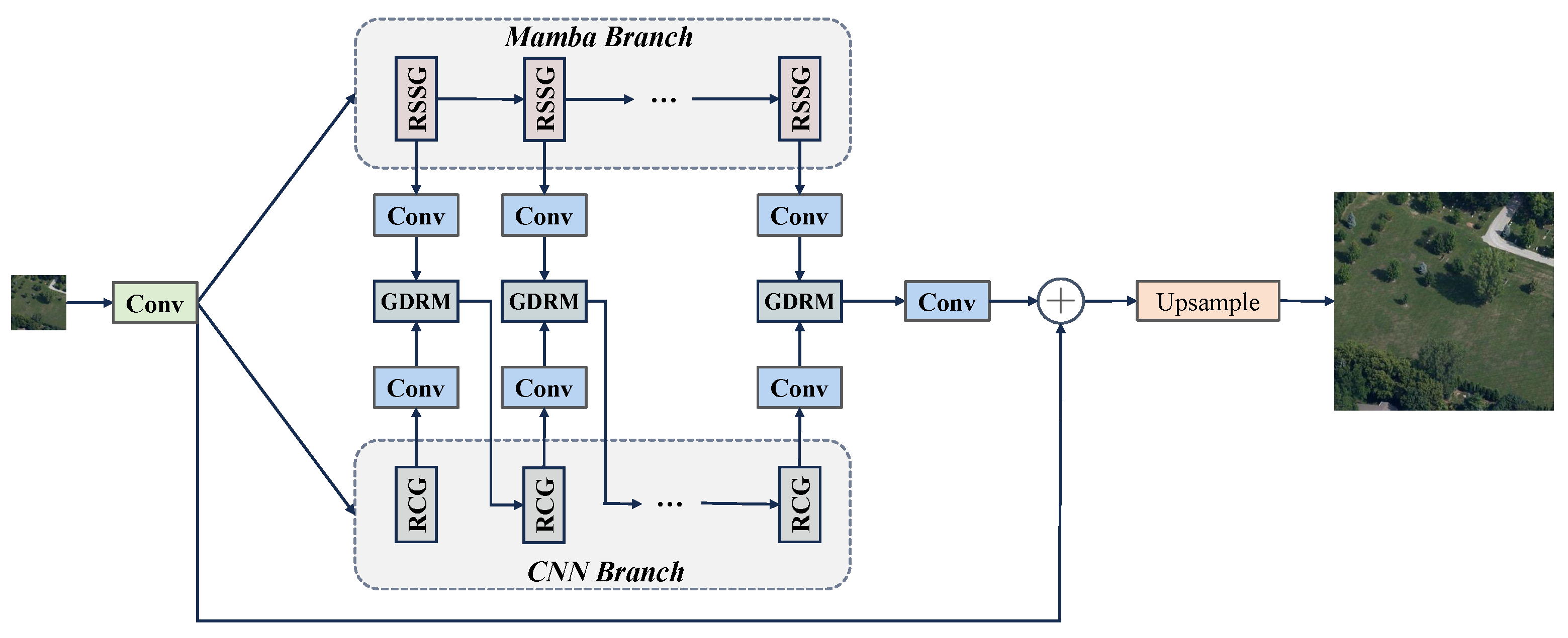
- ConvMambaSR is proposed as a hybrid model combining CNN and Mamba. It employs a dual-branch architecture: the CNN branch extracts local features and processes spatial information, while the Mamba branch captures global features and long-range dependencies.
- A global–detail reconstruction module is introduced within ConvMambaSR, designed to integrate local details from the CNN with global contextual information from the Mamba. This module enhances the synergy between the branches by merging local features with global information, thereby improving model performance across various tasks.
2. Related Works
2.1. Advances in SISR and Applications to Remote Sensing
2.2. State-Space Models in Deep Learning
3. Methodology
3.1. Overall Structure of ConvMambaSR
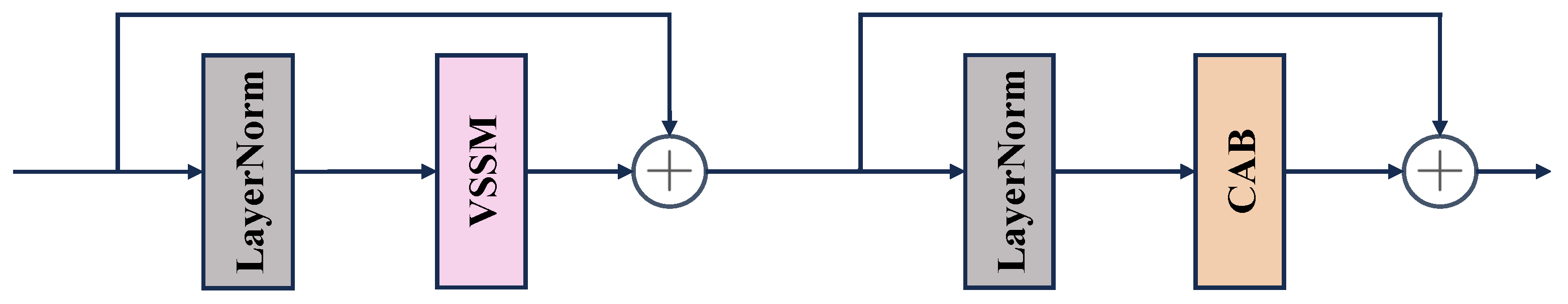
3.2. Residual State-Space Group
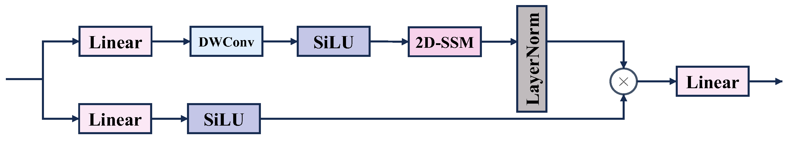
3.2.1. Vision State-Space Module
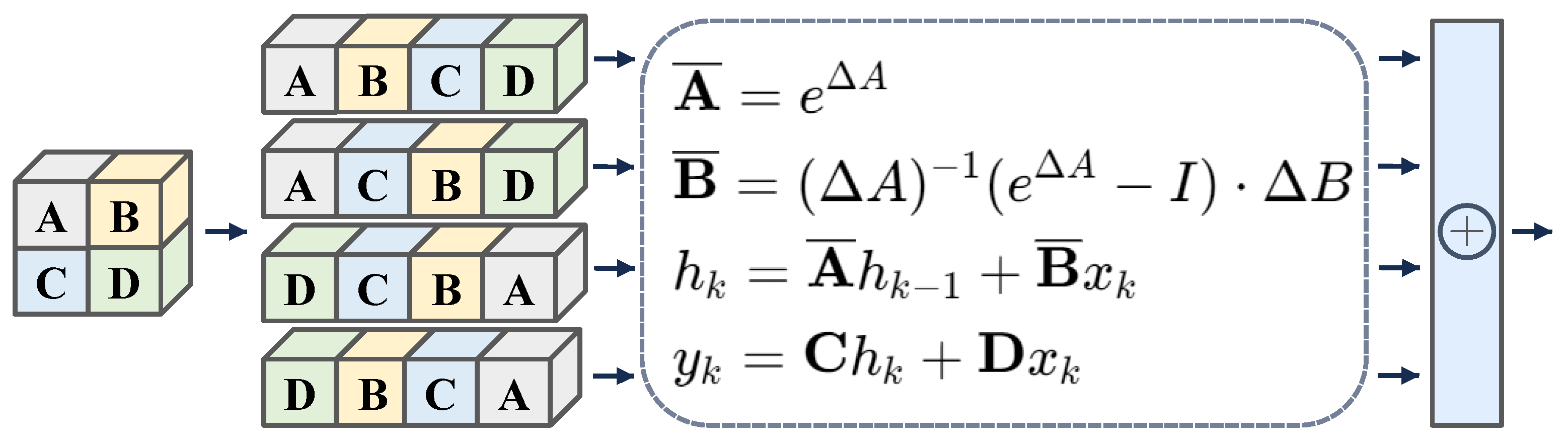
3.2.2. Two-Dimensional Selective Scan Module
3.2.3. Residual State-Space Block
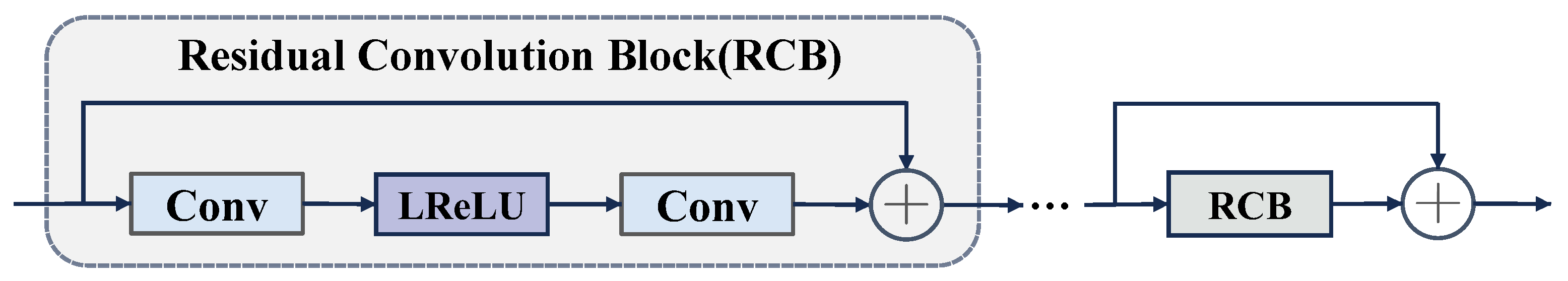
3.3. Residual Convolution Group
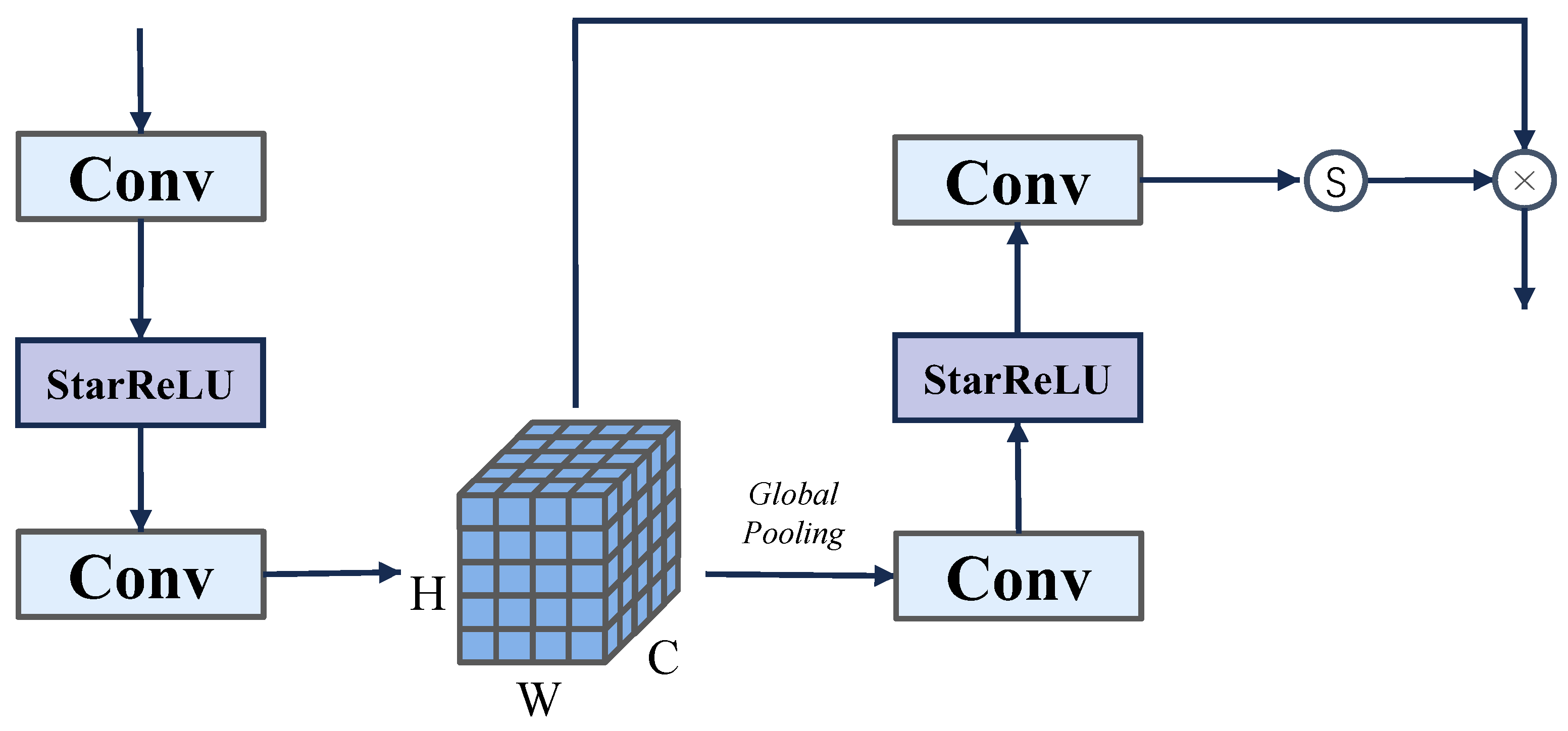
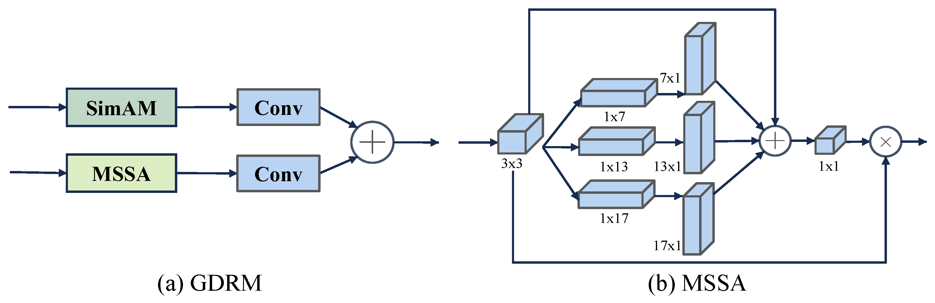
3.4. Global–Detail Reconstruction Module
3.5. Loss Function
4. Experiments
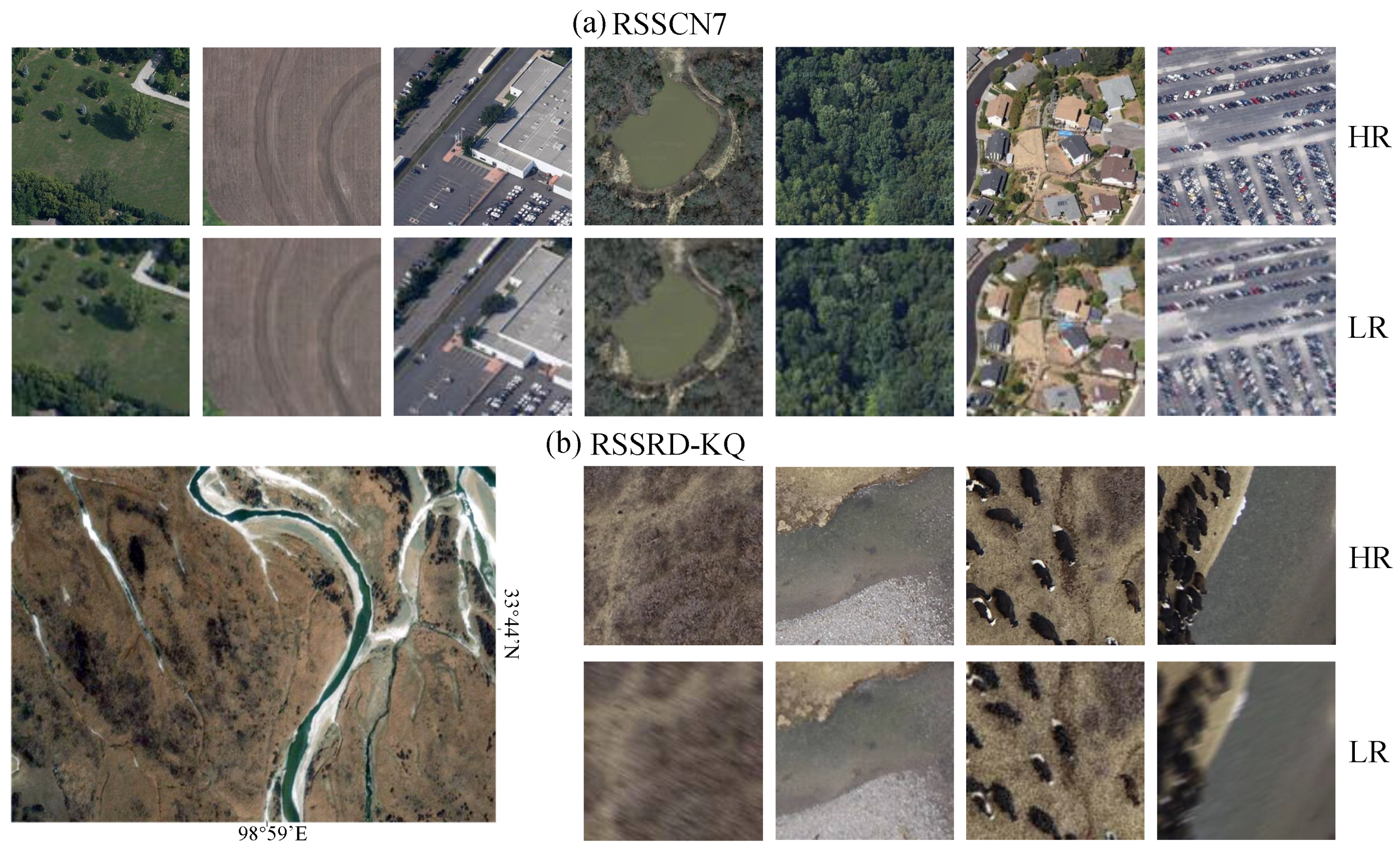
4.1. Datasets
4.2. Experiment Settings
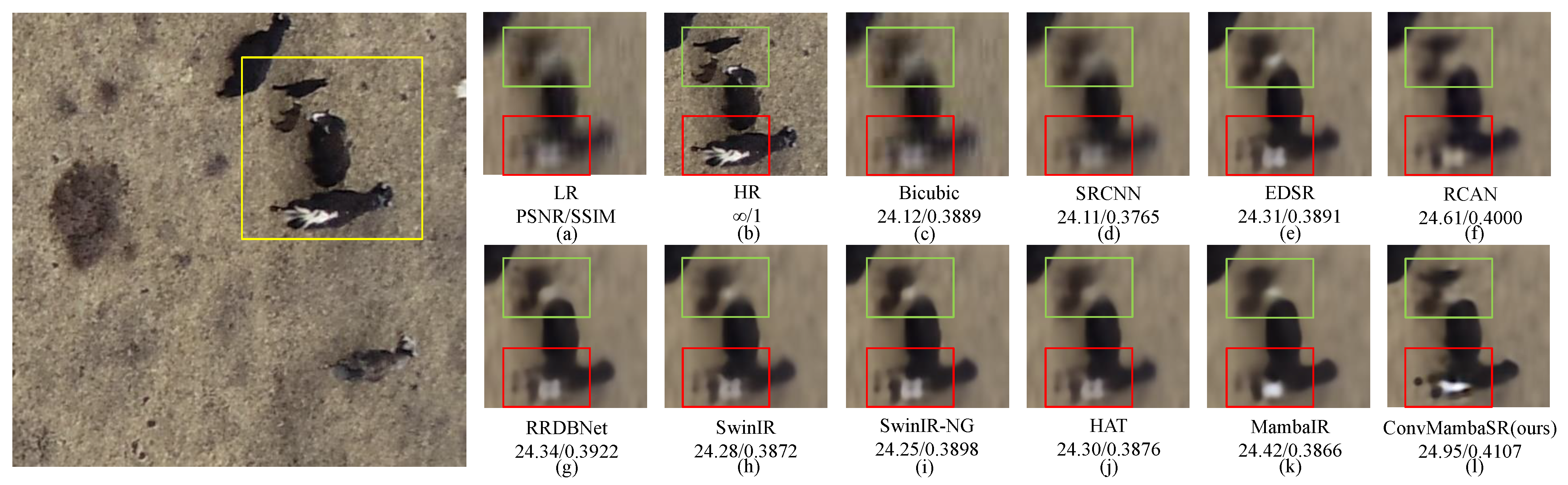
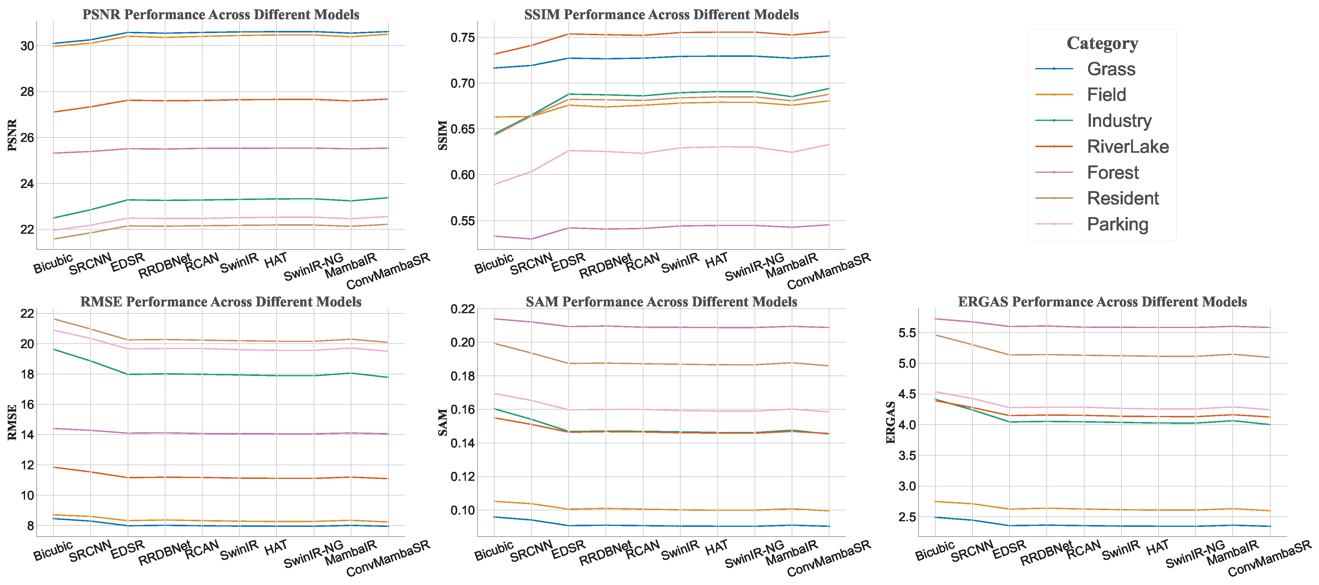
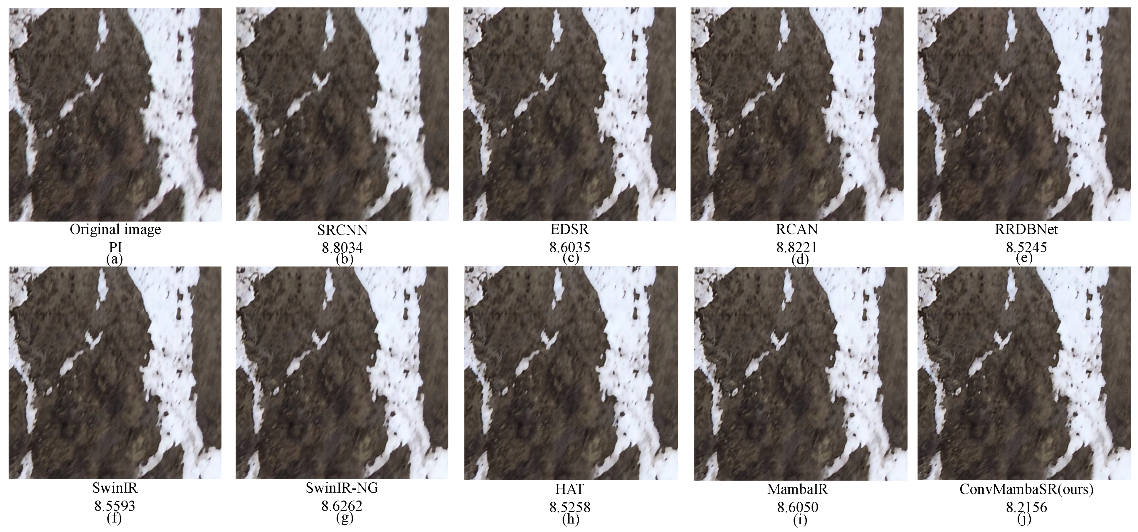
4.3. Results
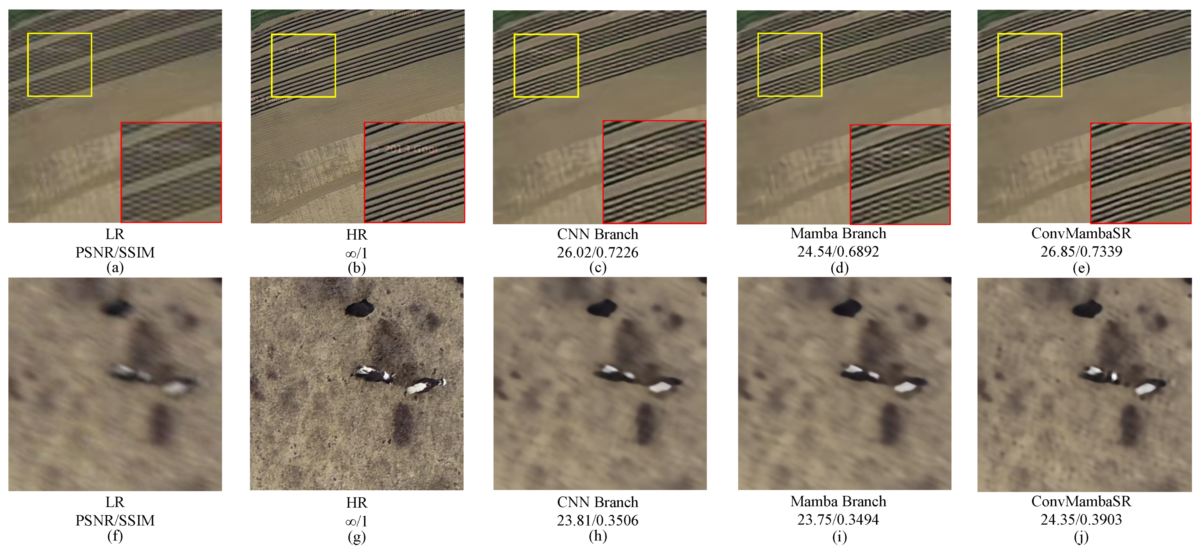
4.4. Effects of GDRM
4.5. Ablation Study on RCG Count
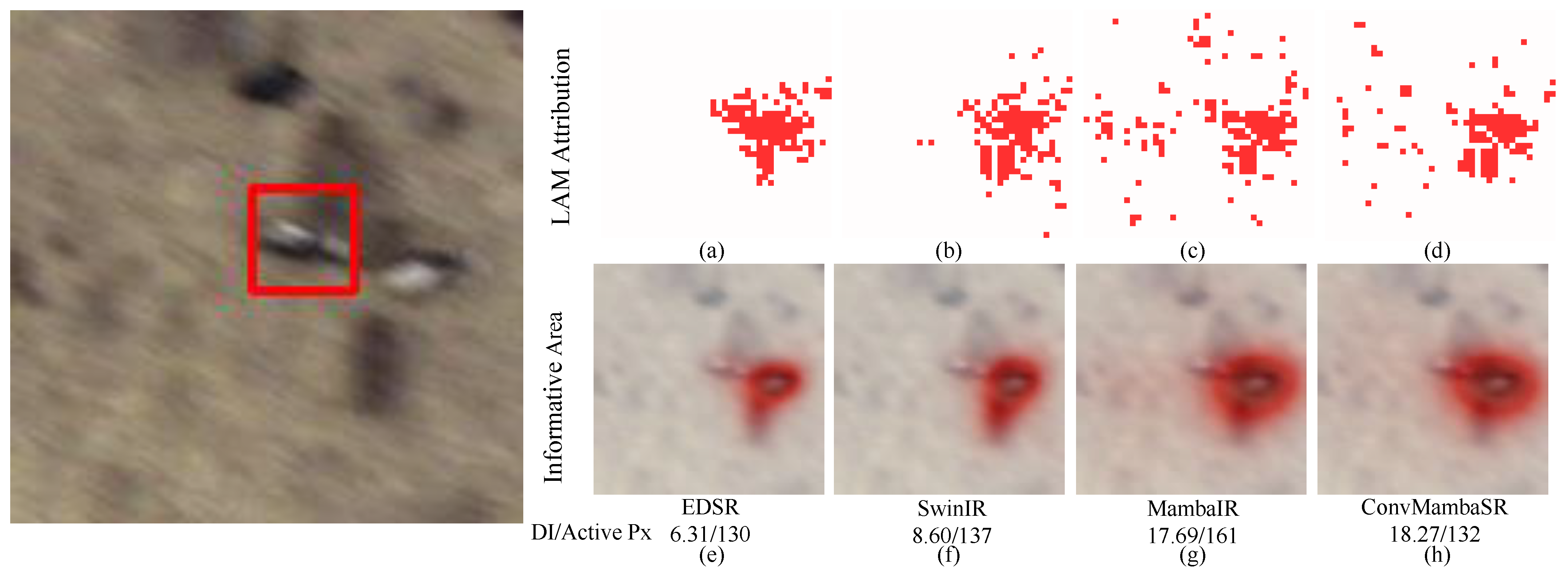
4.6. LAM Analysis and Feature Visualization
4.7. Complexity and Efficiency Evaluation
4.8. Real-World Image Testing
5. Conclusions
Author Contributions
Funding
Data Availability Statement
Conflicts of Interest
References
- Mathieu, R.; Freeman, C.; Aryal, J. Mapping private gardens in urban areas using object-oriented techniques and very high-resolution satellite imagery. Landsc. Urban Plan. 2007, 81, 179–192. [Google Scholar] [CrossRef]
- Kumar, S.; Meena, R.S.; Sheoran, S.; Jangir, C.K.; Jhariya, M.K.; Banerjee, A.; Raj, A. Remote sensing for agriculture and resource management. In Natural Resources Conservation and Advances for Sustainability; Elsevier: Amsterdam, The Netherlands, 2022; pp. 91–135. [Google Scholar]
- Turner, W.; Spector, S.; Gardiner, N.; Fladeland, M.; Sterling, E.; Steininger, M. Remote sensing for biodiversity science and conservation. Trends Ecol. Evol. 2003, 18, 306–314. [Google Scholar] [CrossRef]
- Yang, J.; Gong, P.; Fu, R.; Zhang, M.; Chen, J.; Liang, S.; Xu, B.; Shi, J.; Dickinson, R. The role of satellite remote sensing in climate change studies. Nat. Clim. Chang. 2013, 3, 875–883. [Google Scholar] [CrossRef]
- Li, J.; Pei, Y.; Zhao, S.; Xiao, R.; Sang, X.; Zhang, C. A review of remote sensing for environmental monitoring in China. Remote Sens. 2020, 12, 1130. [Google Scholar] [CrossRef]
- Singh, S.; Bhardwaj, A.; Verma, V. Remote sensing and GIS based analysis of temporal land use/land cover and water quality changes in Harike wetland ecosystem, Punjab, India. J. Environ. Manag. 2020, 262, 110355. [Google Scholar] [CrossRef]
- Soubry, I.; Doan, T.; Chu, T.; Guo, X. A systematic review on the integration of remote sensing and GIS to forest and grassland ecosystem health attributes, indicators, and measures. Remote Sens. 2021, 13, 3262. [Google Scholar] [CrossRef]
- Bhaga, T.D.; Dube, T.; Shekede, M.D.; Shoko, C. Impacts of climate variability and drought on surface water resources in Sub-Saharan Africa using remote sensing: A review. Remote Sens. 2020, 12, 4184. [Google Scholar] [CrossRef]
- Wang, P.; Bayram, B.; Sertel, E. A comprehensive review on deep learning based remote sensing image super-resolution methods. Earth-Sci. Rev. 2022, 232, 104110. [Google Scholar] [CrossRef]
- Li, K.; Yang, S.; Dong, R.; Wang, X.; Huang, J. Survey of single image super-resolution reconstruction. IET Image Process. 2020, 14, 2273–2290. [Google Scholar] [CrossRef]
- Wang, Y.; Bashir, S.M.A.; Khan, M.; Ullah, Q.; Wang, R.; Song, Y.; Guo, Z.; Niu, Y. Remote sensing image super-resolution and object detection: Benchmark and state of the art. Expert Syst. Appl. 2022, 197, 116793. [Google Scholar] [CrossRef]
- Yang, W.; Zhang, X.; Tian, Y.; Wang, W.; Xue, J.H.; Liao, Q. Deep learning for single image super-resolution: A brief review. IEEE Trans. Multimed. 2019, 21, 3106–3121. [Google Scholar] [CrossRef]
- He, K.; Zhang, X.; Ren, S.; Sun, J. Deep residual learning for image recognition. In Proceedings of the IEEE Conference on Computer Vision and Pattern Recognition, Las Vegas, NV, USA, 27–30 June 2016; pp. 770–778. [Google Scholar]
- Tong, T.; Li, G.; Liu, X.; Gao, Q. Image super-resolution using dense skip connections. In Proceedings of the IEEE International Conference on Computer Vision, Venice, Italy, 22–29 October 2017; pp. 4799–4807. [Google Scholar]
- Goodfellow, I.; Pouget-Abadie, J.; Mirza, M.; Xu, B.; Warde-Farley, D.; Ozair, S.; Courville, A.; Bengio, Y. Generative adversarial networks. Commun. ACM 2020, 63, 139–144. [Google Scholar] [CrossRef]
- Zhang, Y.; Li, K.; Li, K.; Wang, L.; Zhong, B.; Fu, Y. Image super-resolution using very deep residual channel attention networks. In Proceedings of the European Conference on Computer Vision (ECCV), Munich, Germany, 8–14 September 2018; pp. 286–301. [Google Scholar]
- He, X.; Zhou, Y.; Zhao, J.; Zhang, D.; Yao, R.; Xue, Y. Swin transformer embedding UNet for remote sensing image semantic segmentation. IEEE Trans. Geosci. Remote Sens. 2022, 60, 1–15. [Google Scholar] [CrossRef]
- Dong, C.; Loy, C.C.; He, K.; Tang, X. Image super-resolution using deep convolutional networks. IEEE Trans. Pattern Anal. Mach. Intell. 2015, 38, 295–307. [Google Scholar] [CrossRef] [PubMed]
- Lim, B.; Son, S.; Kim, H.; Nah, S.; Mu Lee, K. Enhanced deep residual networks for single image super-resolution. In Proceedings of the IEEE Conference on Computer Vision and Pattern Recognition Workshops, Honolulu, HI, USA, 21–26 July 2017; pp. 136–144. [Google Scholar]
- Liang, J.; Cao, J.; Sun, G.; Zhang, K.; Van Gool, L.; Timofte, R. Swinir: Image restoration using swin transformer. In Proceedings of the IEEE/CVF international Conference on Computer Vision, Montreal, BC, Canada, 11–17 October 2021; pp. 1833–1844. [Google Scholar]
- Chen, B.; Zou, X.; Zhang, Y.; Li, J.; Li, K.; Xing, J.; Tao, P. LEFormer: A Hybrid CNN-Transformer Architecture for Accurate Lake Extraction from Remote Sensing Imagery. In Proceedings of the ICASSP 2024—2024 IEEE International Conference on Acoustics, Speech and Signal Processing (ICASSP), Seoul, Republic of Korea, 14–19 April 2024; pp. 5710–5714. [Google Scholar]
- Zou, X.; Li, K.; Xing, J.; Zhang, Y.; Wang, S.; Jin, L.; Tao, P. DiffCR: A Fast Conditional Diffusion Framework for Cloud Removal From Optical Satellite Images. IEEE Trans. Geosci. Remote Sens. 2024, 62, 1–14. [Google Scholar] [CrossRef]
- Wang, S.; Zou, X.; Li, K.; Xing, J.; Cao, T.; Tao, P. Towards robust pansharpening: A large-scale high-resolution multi-scene dataset and novel approach. Remote Sens. 2024, 16, 62899. [Google Scholar] [CrossRef]
- Li, K.; Xie, F.; Chen, H.; Yuan, K.; Hu, X. An audio-visual speech separation model inspired by cortico-thalamo-cortical circuits. IEEE Trans. Pattern Anal. Mach. Intell. 2024, 1–15. [Google Scholar] [CrossRef]
- Zou, X.; Li, K.; Xing, J.; Tao, P.; Cui, Y. PMAA: A Progressive Multi-scale Attention Autoencoder Model for High-Performance Cloud Removal from Multi-temporal Satellite Imagery. In Proceedings of the European Conference on Artificial Intelligence (ECAI), Kraków, Poland, 30 September–4 October 2023; pp. 3165–3172. [Google Scholar]
- Vaswani, A.; Shazeer, N.; Parmar, N.; Uszkoreit, J.; Jones, L.; Gomez, A.N.; Kaiser, Ł.; Polosukhin, I. Attention is all you need. Adv. Neural Inf. Process. Syst. 2017, 30. [Google Scholar]
- Liu, Z.; Lin, Y.; Cao, Y.; Hu, H.; Wei, Y.; Zhang, Z.; Lin, S.; Guo, B. Swin transformer: Hierarchical vision transformer using shifted windows. In Proceedings of the IEEE/CVF International Conference on Computer Vision, Montreal, BC, Canada, 11–17 October 2021; pp. 10012–10022. [Google Scholar]
- Gao, L.; Liu, H.; Yang, M.; Chen, L.; Wan, Y.; Xiao, Z.; Qian, Y. STransFuse: Fusing swin transformer and convolutional neural network for remote sensing image semantic segmentation. IEEE J. Sel. Top. Appl. Earth Obs. Remote Sens. 2021, 14, 10990–11003. [Google Scholar] [CrossRef]
- Fu, D.Y.; Dao, T.; Saab, K.K.; Thomas, A.W.; Rudra, A.; Ré, C. Hungry hungry hippos: Towards language modeling with state space models. arXiv 2022, arXiv:2212.14052. [Google Scholar]
- Gu, A.; Dao, T. Mamba: Linear-time sequence modeling with selective state spaces. arXiv 2023, arXiv:2312.00752. [Google Scholar]
- Mehta, H.; Gupta, A.; Cutkosky, A.; Neyshabur, B. Long range language modeling via gated state spaces. arXiv 2022, arXiv:2206.13947. [Google Scholar]
- Smith, J.T.; Warrington, A.; Linderman, S.W. Simplified state space layers for sequence modeling. arXiv 2022, arXiv:2208.04933. [Google Scholar]
- Li, K.; Chen, G. Spmamba: State-space model is all you need in speech separation. arXiv 2024, arXiv:2404.02063. [Google Scholar]
- Gu, A.; Dao, T.; Ermon, S.; Rudra, A.; Ré, C. Hippo: Recurrent memory with optimal polynomial projections. Adv. Neural Inf. Process. Syst. 2020, 33, 1474–1487. [Google Scholar]
- Shi, W.; Caballero, J.; Huszár, F.; Totz, J.; Aitken, A.P.; Bishop, R.; Rueckert, D.; Wang, Z. Real-time single image and video super-resolution using an efficient sub-pixel convolutional neural network. In Proceedings of the IEEE Conference on Computer Vision and Pattern Recognition, Las Vegas, NV, USA, 27–30 June 2016; pp. 1874–1883. [Google Scholar]
- Ledig, C.; Theis, L.; Huszár, F.; Caballero, J.; Cunningham, A.; Acosta, A.; Aitken, A.; Tejani, A.; Totz, J.; Wang, Z.; et al. Photo-realistic single image super-resolution using a generative adversarial network. In Proceedings of the IEEE Conference on Computer Vision and Pattern Recognition, Honolulu, HI, USA, 21–26 July 2017; pp. 4681–4690. [Google Scholar]
- Wang, X.; Yu, K.; Wu, S.; Gu, J.; Liu, Y.; Dong, C.; Qiao, Y.; Change Loy, C. Esrgan: Enhanced super-resolution generative adversarial networks. In Proceedings of the European Conference on Computer Vision (ECCV) Workshops, Munich, Germany, 8–14 September 2018. [Google Scholar]
- Niu, B.; Wen, W.; Ren, W.; Zhang, X.; Yang, L.; Wang, S.; Zhang, K.; Cao, X.; Shen, H. Single image super-resolution via a holistic attention network. In Proceedings of the Computer Vision–ECCV 2020: 16th Europea Conference, Proceedings Part XII 16, Glasgow, UK, 23–28 August 2020; Springer: Cham, Switzerland, 2020; pp. 191–207. [Google Scholar]
- Huang, J.; Li, K.; Wang, X. Single image super-resolution reconstruction of enhanced loss function with multi-gpu training. In Proceedings of the 2019 IEEE Intl Conf on Parallel & Distributed Processing with Applications, Big Data & Cloud Computing, Sustainable Computing & Communications, Social Computing & Networking (ISPA/BDCloud/SocialCom/SustainCom), Xiamen, China, 16–18 December 2019; pp. 559–565. [Google Scholar]
- Dosovitskiy, A.; Beyer, L.; Kolesnikov, A.; Weissenborn, D.; Zhai, X.; Unterthiner, T.; Dehghani, M.; Minderer, M.; Heigold, G.; Gelly, S.; et al. An image is worth 16 × 16 words: Transformers for image recognition at scale. arXiv 2020, arXiv:2010.11929. [Google Scholar]
- Chen, X.; Wang, X.; Zhou, J.; Qiao, Y.; Dong, C. Activating more pixels in image super-resolution transformer. In Proceedings of the IEEE/CVF Conference on Computer Vision and Pattern Recognition, Vancouver, BC, Canada, 17–24 June 2023; pp. 22367–22377. [Google Scholar]
- Choi, H.; Lee, J.; Yang, J. N-gram in swin transformers for efficient lightweight image super-resolution. In Proceedings of the IEEE/CVF Conference on Computer Vision and Pattern Recognition, Vancouver, BC, Canada, 17–24 June 2023; pp. 2071–2081. [Google Scholar]
- Fernandez-Beltran, R.; Latorre-Carmona, P.; Pla, F. Single-frame super-resolution in remote sensing: A practical overview. Int. J. Remote Sens. 2017, 38, 314–354. [Google Scholar] [CrossRef]
- Ducournau, A.; Fablet, R. Deep learning for ocean remote sensing: An application of convolutional neural networks for super-resolution on satellite-derived SST data. In Proceedings of the IEEE 2016 9th IAPR Workshop on Pattern Recogniton in Remote Sensing (PRRS), Cancun, Mexico, 4 December 2016; pp. 1–6. [Google Scholar]
- Pan, Z.; Ma, W.; Guo, J.; Lei, B. Super-resolution of single remote sensing image based on residual dense backprojection networks. IEEE Trans. Geosci. Remote Sens. 2019, 57, 7918–7933. [Google Scholar] [CrossRef]
- Huan, H.; Li, P.; Zou, N.; Wang, C.; Xie, Y.; Xie, Y.; Xu, D. End-to-end super-resolution for remote-sensing images using an improved multi-scale residual network. Remote Sens. 2021, 13, 666. [Google Scholar] [CrossRef]
- Tu, J.; Mei, G.; Ma, Z.; Piccialli, F. SWCGAN: Generative adversarial network combining swin transformer and CNN for remote sensing image super-resolution. IEEE J. Sel. Top. Appl. Earth Obs. Remote Sens. 2022, 15, 5662–5673. [Google Scholar] [CrossRef]
- Shang, J.; Gao, M.; Li, Q.; Pan, J.; Zou, G.; Jeon, G. Hybrid-Scale Hierarchical Transformer for Remote Sensing Image Super-Resolution. Remote Sens. 2023, 15, 3442. [Google Scholar] [CrossRef]
- Li, J.; Meng, Y.; Tao, C.; Zhang, Z.; Yang, X.; Wang, Z.; Wang, X.; Li, L.; Zhang, W. ConvFormerSR: Fusing Transformers and Convolutional Neural Networks for Cross-sensor Remote Sensing Imagery Super-resolution. IEEE Trans. Geosci. Remote Sens. 2023, 62, 5601115. [Google Scholar] [CrossRef]
- Gu, A.; Goel, K.; Ré, C. Efficiently modeling long sequences with structured state spaces. arXiv 2021, arXiv:2111.00396. [Google Scholar]
- Gu, A.; Johnson, I.; Goel, K.; Saab, K.; Dao, T.; Rudra, A.; Ré, C. Combining recurrent, convolutional, and continuous-time models with linear state space layers. Adv. Neural Inf. Process. Syst. 2021, 34, 572–585. [Google Scholar]
- Chen, H.; Wang, Y.; Guo, T.; Xu, C.; Deng, Y.; Liu, Z.; Ma, S.; Xu, C.; Xu, C.; Gao, W. Pre-trained image processing transformer. In Proceedings of the IEEE/CVF Conference on Computer Vision and Pattern Recognition, Nashville, TN, USA, 20–25 June 2021; pp. 12299–12310. [Google Scholar]
- Liu, Y.; Tian, Y.; Zhao, Y.; Yu, H.; Xie, L.; Wang, Y.; Ye, Q.; Liu, Y. Vmamba: Visual state space model. arXiv 2024, arXiv:2401.10166. [Google Scholar]
- Shazeer, N. Glu variants improve transformer. arXiv 2020, arXiv:2002.05202. [Google Scholar]
- Guo, H.; Li, J.; Dai, T.; Ouyang, Z.; Ren, X.; Xia, S.T. MambaIR: A Simple Baseline for Image Restoration with State-Space Model. arXiv 2024, arXiv:2402.15648. [Google Scholar]
- Hu, J.; Shen, L.; Sun, G. Squeeze-and-excitation networks. In Proceedings of the IEEE Conference on Computer Vision and Pattern Recognition, Salt Lake City, UT, USA, 18–23 June 2018; pp. 7132–7141. [Google Scholar]
- Yu, W.; Si, C.; Zhou, P.; Luo, M.; Zhou, Y.; Feng, J.; Yan, S.; Wang, X. Metaformer baselines for vision. IEEE Trans. Pattern Anal. Mach. Intell. 2023, 46, 896–912. [Google Scholar] [CrossRef]
- Li, K.; Yang, R.; Sun, F.; Hu, X. IIANet: An Intra-and Inter-Modality Attention Network for Audio-Visual Speech Separation. In Proceedings of the Forty-First International Conference on Machine Learning, Vienna, Austria, 21–27 July 2024. [Google Scholar]
- Guo, M.H.; Lu, C.Z.; Hou, Q.; Liu, Z.; Cheng, M.M.; Hu, S.M. Segnext: Rethinking convolutional attention design for semantic segmentation. Adv. Neural Inf. Process. Syst. 2022, 35, 1140–1156. [Google Scholar]
- Yang, L.; Zhang, R.Y.; Li, L.; Xie, X. Simam: A simple, parameter-free attention module for convolutional neural networks. In Proceedings of the International Conference on Machine Learning, PMLR, Virtual, 18–24 July 2021; pp. 11863–11874. [Google Scholar]
- Peng, C.; Zhang, X.; Yu, G.; Luo, G.; Sun, J. Large kernel matters–improve semantic segmentation by global convolutional network. In Proceedings of the IEEE Conference on Computer Vision and Pattern Recognition, Honolulu, HI, USA, 21–26 July 2017; pp. 4353–4361. [Google Scholar]
- Hou, Q.; Zhang, L.; Cheng, M.M.; Feng, J. Strip pooling: Rethinking spatial pooling for scene parsing. In Proceedings of the IEEE/CVF Conference on Computer Vision and Pattern Recognition, Seattle, WA, USA, 13–19 June 2020; pp. 4003–4012. [Google Scholar]
- Li, K.; Luo, Y. On the design and training strategies for rnn-based online neural speech separation systems. In Proceedings of the ICASSP 2023–2023 IEEE International Conference on Acoustics, Speech and Signal Processing (ICASSP), Rhodes, Greece, 4–10 June 2023; pp. 1–5. [Google Scholar]
- Zou, Q.; Ni, L.; Zhang, T.; Wang, Q. Deep learning based feature selection for remote sensing scene classification. IEEE Geosci. Remote Sens. Lett. 2015, 12, 2321–2325. [Google Scholar] [CrossRef]
- Zhang, K.; Liang, J.; Van Gool, L.; Timofte, R. Designing a practical degradation model for deep blind image super-resolution. In Proceedings of the IEEE/CVF International Conference on Computer Vision, Montreal, BC, Canada, 11–17 October 2021; pp. 4791–4800. [Google Scholar]
- Wang, X.; Xie, L.; Dong, C.; Shan, Y. Real-esrgan: Training real-world blind super-resolution with pure synthetic data. In Proceedings of the IEEE/CVF International Conference on Computer Vision, Montreal, BC, Canada, 11–17 October 2021; pp. 1905–1914. [Google Scholar]
- Wang, Z.; Bovik, A.C.; Sheikh, H.R.; Simoncelli, E.P. Image quality assessment: From error visibility to structural similarity. IEEE Trans. Image Process. 2004, 13, 600–612. [Google Scholar] [CrossRef] [PubMed]
- Yuhas, R.H.; Goetz, A.F.; Boardman, J.W. Discrimination among semi-arid landscape endmembers using the spectral angle mapper (SAM) algorithm. In Proceedings of the JPL, Summaries of the Third Annual JPL Airborne Geoscience Workshop; Volume 1: AVIRIS Workshop, Pasadena, CA, USA, 1–5 June 1992. [Google Scholar]
- Ranchin, T.; Wald, L. Fusion of high spatial and spectral resolution images: The ARSIS concept and its implementation. Photogramm. Eng. Remote Sens. 2000, 66, 49–61. [Google Scholar]
- Blau, Y.; Mechrez, R.; Timofte, R.; Michaeli, T.; Zelnik-Manor, L. The 2018 PIRM challenge on perceptual image super-resolution. In Proceedings of the European Conference on Computer Vision (ECCV) Workshops, Munich, Germany, 8–14 September l2018. [Google Scholar]
- Ma, C.; Yang, C.Y.; Yang, X.; Yang, M.H. Learning a no-reference quality metric for single-image super-resolution. Comput. Vis. Image Underst. 2017, 158, 1–16. [Google Scholar] [CrossRef]
- Mittal, A.; Soundararajan, R.; Bovik, A.C. Making a “completely blind” image quality analyzer. IEEE Signal Process. Lett. 2012, 20, 209–212. [Google Scholar] [CrossRef]
- Gu, J.; Dong, C. Interpreting super-resolution networks with local attribution maps. In Proceedings of the IEEE/CVF Conference on Computer Vision and Pattern Recognition, Nashville, TN, USA, 20–25 June 2021; pp. 9199–9208. [Google Scholar]
- Sundararajan, M.; Taly, A.; Yan, Q. Axiomatic attribution for deep networks. In Proceedings of the International Conference on Machine Learning, PMLR, Sydney, Australia, 6–11 August 2017; pp. 3319–3328. [Google Scholar]


| Dataset | Method | PSNR (dB)↑ | SSIM↑ | RMSE↓ | SAM↓ | ERGAS↓ |
|---|---|---|---|---|---|---|
| RSSCN7 | Bicubic | 25.50 | 0.6457 | 15.0848 | 0.1570 | 4.2513 |
| SRCNN [18] | 25.70 | 0.6551 | 14.7016 | 0.1534 | 4.1536 | |
| SRGAN [36] | 25.96 | 0.6686 | 14.2594 | 0.1492 | 4.0402 | |
| EDSR [19] | 26.00 | 0.6706 | 14.2090 | 0.1487 | 4.0256 | |
| RRDBNet [14] | 25.98 | 0.6696 | 14.2405 | 0.1489 | 4.0346 | |
| RCAN [16] | 26.00 | 0.6694 | 14.2109 | 0.1487 | 4.0257 | |
| SwinIR [20] | 26.02 | 0.6727 | 14.1720 | 0.1483 | 4.0153 | |
| HAT [41] | 26.04 | 0.6734 | 14.1480 | 0.1481 | 4.0092 | |
| SwinIR-NG [42] | 26.04 | 0.6734 | 14.1453 | 0.1480 | 4.0084 | |
| MambaIR [55] | 25.98 | 0.6697 | 14.2493 | 0.1490 | 4.0363 | |
| ConvMambaSR(ours) | 26.06 | 0.6751 | 14.1029 | 0.1477 | 3.9985 | |
| RSSRD-KQ | Bicubic | 23.74 | 0.3471 | 16.9950 | 0.1495 | 3.8872 |
| SRCNN [18] | 24.06 | 0.3541 | 16.2812 | 0.1435 | 3.7173 | |
| SRGAN [36] | 24.06 | 0.3582 | 16.2846 | 0.1435 | 3.7155 | |
| EDSR [19] | 24.18 | 0.3648 | 16.0725 | 0.1415 | 3.6685 | |
| RRDBNet [14] | 24.19 | 0.3666 | 16.0470 | 0.1414 | 3.6614 | |
| RCAN [16] | 24.27 | 0.3740 | 15.9059 | 0.1404 | 3.6290 | |
| SwinIR [20] | 24.20 | 0.3672 | 16.0310 | 0.1412 | 3.6586 | |
| HAT [41] | 24.21 | 0.3684 | 16.0068 | 0.1411 | 3.6530 | |
| SwinIR-NG [42] | 24.20 | 0.3676 | 16.0305 | 0.1412 | 3.6587 | |
| MambaIR [55] | 24.23 | 0.3663 | 15.9726 | 0.1407 | 3.6450 | |
| ConvMambaSR(ours) | 24.29 | 0.3752 | 15.8632 | 0.1398 | 3.6205 |
| Dataset | Method | PSNR(dB)↑ | SSIM↑ | RMSE↓ | SAM↓ | ERGAS↓ |
|---|---|---|---|---|---|---|
| RSSCN7 | CNN Branch | 26.05 | 0.6740 | 14.1201 | 0.1478 | 4.0032 |
| Mamba Branch | 26.00 | 0.6704 | 14.2115 | 0.1487 | 4.0269 | |
| ConvMambaSR | 26.06 | 0.6751 | 14.1029 | 0.1477 | 3.9985 | |
| RSSRD-KQ | CNN Branch | 24.23 | 0.3698 | 15.9706 | 0.1408 | 3.6443 |
| Mamba Branch | 24.25 | 0.3706 | 15.9296 | 0.1405 | 3.6353 | |
| ConvMambaSR | 24.29 | 0.3752 | 15.8632 | 0.1398 | 3.6205 |
| RCG Count | #Para ms (M) | FLOPs (G) | PSNR (dB)↑ | SSIM↑ |
|---|---|---|---|---|
| 1 | 6.72 | 175 | 26.05 | 0.6742 |
| 4 | 8.71 | 226 | 26.05 | 0.6742 |
| 8 | 11.37 | 294 | 26.06 | 0.6751 |
| 12 | 14.02 | 362 | 26.06 | 0.6751 |
| 16 | 16.68 | 430 | 26.07 | 0.6756 |
| 20 | 19.34 | 498 | 26.07 | 0.6759 |
| Model | #Params (M) | FLOPs (G) | FPS |
|---|---|---|---|
| Bicubic | - | - | 22557.1 |
| SRCNN [18] | 0.02 | 8 | 620.7 |
| EDSR [19] | 1.51 | 50 | 268.0 |
| RRDBNet [14] | 16.69 | 459 | 27.5 |
| RCAN [16] | 15.59 | 408 | 20.6 |
| MambaIR [55] | 4.65 | 123 | 10.3 |
| HAT [41] | 26.03 | 703 | 4.4 |
| SwinIR [20] | 16.57 | 456 | 0.5 |
| SwinIR-NG [42] | 19.35 | 460 | 0.4 |
| ConvMambaSR(ours) | 14.02 | 362 | 8.9 |
Disclaimer/Publisher’s Note: The statements, opinions and data contained in all publications are solely those of the individual author(s) and contributor(s) and not of MDPI and/or the editor(s). MDPI and/or the editor(s) disclaim responsibility for any injury to people or property resulting from any ideas, methods, instructions or products referred to in the content. |
© 2024 by the authors. Licensee MDPI, Basel, Switzerland. This article is an open access article distributed under the terms and conditions of the Creative Commons Attribution (CC BY) license (https://creativecommons.org/licenses/by/4.0/).
Share and Cite
Zhu, Q.; Zhang, G.; Zou, X.; Wang, X.; Huang, J.; Li, X. ConvMambaSR: Leveraging State-Space Models and CNNs in a Dual-Branch Architecture for Remote Sensing Imagery Super-Resolution. Remote Sens. 2024, 16, 3254. https://doi.org/10.3390/rs16173254
Zhu Q, Zhang G, Zou X, Wang X, Huang J, Li X. ConvMambaSR: Leveraging State-Space Models and CNNs in a Dual-Branch Architecture for Remote Sensing Imagery Super-Resolution. Remote Sensing. 2024; 16(17):3254. https://doi.org/10.3390/rs16173254
Chicago/Turabian StyleZhu, Qiwei, Guojing Zhang, Xuechao Zou, Xiaoying Wang, Jianqiang Huang, and Xilai Li. 2024. "ConvMambaSR: Leveraging State-Space Models and CNNs in a Dual-Branch Architecture for Remote Sensing Imagery Super-Resolution" Remote Sensing 16, no. 17: 3254. https://doi.org/10.3390/rs16173254
APA StyleZhu, Q., Zhang, G., Zou, X., Wang, X., Huang, J., & Li, X. (2024). ConvMambaSR: Leveraging State-Space Models and CNNs in a Dual-Branch Architecture for Remote Sensing Imagery Super-Resolution. Remote Sensing, 16(17), 3254. https://doi.org/10.3390/rs16173254