A New Data Fusion Method for GNSS/INS Integration Based on Weighted Multiple Criteria

Abstract

The standard Kalman filter and most of its enhancements are typically designed based on the criterion that minimizes the mean squared error, with little discussion of multiple criteria in the positioning and navigation fields. Therefore, a novel data fusion method that takes into account weighted multiple criteria is proposed in this paper, implementing a filtering algorithm based on integrated criteria with different weights determined by a weight adjustment factor. The proposed algorithm and conventional filtering algorithms were utilized for data fusion in GNSS/INS integration. Experiments were conducted using actual data collected from an urban environment. Comparative analysis revealed that, when utilizing the proposed algorithm, the precision of the position, velocity, and attitude of the tested land vehicle could be improved by approximately 24%, 48%, and 35%, respectively. Furthermore, a series of filtering algorithms with different weight adjustment factors was performed to test their influence on the filtering. The application of the proposed algorithm should be accompanied by an appropriate weight adjustment factor.

1. Introduction

Precise position, velocity, and time information can be obtained with the GNSS technique, which has been widely applied in broad fields [1,2,3]. The precise information is obtained by receiving valid electromagnetic wave signals from an adequate number of visible satellites. However, the satellite signal problem is a persistent challenge due to the fundamental principles underlying positioning with GNSS, and many disturbances exist throughout the practical positioning process. In contrast, the INS technique operates without reliance on external signals, and no signals are transmitted or received by the inertial measurement unit (IMU). Nevertheless, due to the rapid error accumulation inherent to its design limitations, the INS technique cannot deliver long-term, precise navigation and positioning independently. Consequently, INS can serve as the complement of GNSS, leading to the emergence of GNSS/INS integrated navigation systems as a prominent area of interest for many years [4]. Various applications have tested the validity of the GNSS/INS integrated navigation systems [5,6].

In high-dynamic geodetic applications with GNSS/INS integrated navigation systems, the fusion of different types of data from different sensors is one of the primary and key problems. Therefore, a suitable filtering algorithm must be employed to estimate unknown parameters. The Kalman filter is one of the most mature and commonly used state estimation algorithms, and it has been widely applied in parameter estimation for dynamic positioning and navigation [3,7]. However, the standard Kalman filter is only appropriate for linear systems, and statistical information on noise should be known and Gaussian-distributed to achieve optimal results [8]. Otherwise, filtering performance may be degraded or filter divergence may occur. Many improved Kalman filters have been developed and implemented in dynamic positioning and navigation to address these limitations. Overall, integrating advanced technologies such as GNSS and INS presents both opportunities and challenges within high-precision navigation applications, and ongoing research efforts aim to optimize their combined capabilities while mitigating inherent limitations.

Firstly, advanced Kalman filters, such as the extended Kalman filter, unscented Kalman filter, and cubature Kalman filter, have been developed and implemented in GNSS/INS integrated navigation systems to address model nonlinearity issues. The extended Kalman filter linearizes nonlinear functions by preserving only first-order items [9], while the unscented Kalman filter uses unscented transformation (UT) to approximate a Gaussian distribution with a fixed number of parameters [10]. Similarly, the cubature Kalman filter utilizes an even number of cubature points to approximate a Gaussian distribution while ensuring positive weights, even in high-dimensional state space [11,12]. Generally, in terms of observability, the cubature Kalman filter demonstrates comparable or superior performance compared to the extended Kalman filter, and the cubature Kalman filter is suitable for high-dimensional systems, such as the GNSS/INS integrated navigation applications [13]. As nonlinear characteristics are prevalent in many practical systems, there is an expanding application scope for these advanced nonlinear Kalman filters.

Secondly, in practice, the applicability of the Gaussian distribution may not always be guaranteed. It is extremely difficult to determine the exact distribution or density function for most practical scenarios [14], as different applications can result in varying deviations and a complex and dynamic distribution or density function. Consequently, a series of adaptive filters have been developed and applied to address model errors arising from non-Gaussian distributions. For GNSS/INS integrated navigation systems and other high-dynamic navigation and positioning systems, innovation-based adaptive estimation algorithms are considered more suitable [15,16]. The Sage–Husa adaptive filter was introduced using a moving window estimation with an iterative covariance matrix. However, determining the appropriate length of the window poses a challenge [17]. The fading filter is one type of adaptive filter that incorporates a fading factor and has been implemented within navigation and positioning fields. Regarding the fading filter, its primary objective lies in identifying an optimal fading factor [18]. Furthermore, another type of adaptive filter has been developed and applied, which utilizes four distinct error detection statistics along with four different adaptive factors [19].

Thirdly, aiming at the problems posed by outlying measurements and uncertain disturbances, a series of sophisticated filters, known as robust filters, has been developed and implemented within the dynamic navigation and positioning fields. However, it is important to note that both outlier detection algorithms and median-based robust algorithms often suffer from suboptimal efficiency [20]. Nevertheless, this issue can be mitigated through the accurate removal of outliers [21]. Building upon the foundation of outlier detection, methods such as Detection, Identification, and Adaptation (DIA) have been proposed. However, the process of identification is intricate and difficult, leading to the limited application of DIA methods. In terms of robust filters, M-estimation-based approaches have been developed to effectively control the impact of outlying measurements by down-weighting them with an adjustment factor [22]. Additionally, in response to uncertain observation noises, the H∞ filter has been introduced and utilized. Although this filter demonstrates resilience against uncertain observation noises, its performance may still be compromised by outliers [23]. To comprehensively address these challenges, an adaptive and robust Kalman filter has been proposed, which integrates adaptive factors with M-estimation methods to consider both adaptation and robustness [24]. It should be noted that this particular filter requires a sufficient number of measurements that exceed the dimensionality of the state. Based on the H∞ filter and the cubature Kalman filter, a mixed cubature H∞ filter was proposed [25], where the linear H∞ filter was developed into a nonlinear H∞ filter based on the cubature Kalman filter. Certainly, there are other adaptive and improved filters not covered and discussed here due to the space limitations of this paper.

As summarized in the above discussions, various researchers have made great contributions to the filtering algorithms. However, most filtering algorithms for the dynamic navigation and positioning fields are executed based on a fixed and specific criterion, and the performance of most current filtering algorithms is enhanced within this constrained and predetermined framework. Consequently, there has been limited discussion and experimentation on filtering with multiple criteria within the dynamic navigation and positioning fields, and these algorithms were seldom applied in the data fusion of GNSS/INS integrated navigation systems. However, in the fields of mathematical programming and computational science, multiple-criteria-based filtering algorithms have been utilized, with their validation being tested and confirmed [26], and global convergence has been proved [27]. From this perspective, compared to traditional filtering algorithms, employing filtering algorithms based on multiple criteria may offer an alternative avenue for enhancing the filtering performance of GNSS/INS integrated navigation systems. Therefore, a new data fusion algorithm is proposed based on multiple criteria, wherein different criteria are weighted through adjustment factors. Different experiments are devised and conducted using actual data collected from GNSS/INS integrated systems to evaluate both the proposed algorithm and the conventional filtering algorithms.

The remainder of this paper is organized as follows: First, the basic theory of the conventional cubature Kalman and H∞ filters is introduced, and the nonlinear H∞ filter is provided. Second, the dynamic model and the measurement model of the GNSS/INS integrated navigation systems are discussed, and a flowchart of the proposed filtering estimation algorithm is provided. Third, different experiments are designed and implemented to test the performance of the different filtering algorithms. Lastly, the corresponding conclusions are summarized and demonstrated.

2. Related Theory of the Cubature Kalman Filter and the H∞ Filter

The cubature Kalman filter has been adopted in the data fusion of GNSS/INS integrated navigation systems. However, due to the high-dynamic environment and multisensor integration, the uncertainties of these integrated systems tend to increase. Therefore, this paper adopts both the cubature Kalman filter and the H∞ filter as examples to test the effectiveness of the proposed weighted-multiple-criteria-based estimation algorithm and to achieve improved filtering performance in geodetic applications.

The application of the cubature Kalman filter in addressing nonlinear problems within GNSS/INS integrated navigation systems is explored in this paper. In the parameter estimation experiments of this paper, the criteria of the cubature Kalman filter and the H∞ filter are considered and taken as examples to implement the weighted-multiple-criteria-based algorithms. Thus, this section aims to establish fundamental principles for utilizing both the cubature Kalman filter and the H∞ filter effectively.

2.1. Models of the Cubature Kalman Filter

In the field of data fusion and parameter estimation for GNSS/INS integrated navigation systems, the conventional Kalman filter serves as the foundational framework. Building upon this foundation, the cubature Kalman filter and other advanced nonlinear filters have been developed. The cubature Kalman filter, in particular, was formulated based on the principles of spherical-radial cubature. This innovative approach allows for the propagation of both state and covariance matrices with a significantly reduced computational burden compared to the unscented Kalman filter [13]. Nonlinear filtering reduces the problem of how to compute integrals, and the cubature Kalman filter solves the problem by using a set of cubature points with equal weight, and it uses the cubature numerical integration criterion to calculate the mean and covariance matrix of the random variable after nonlinear transformation [11]. For the Gaussian multiple dimension integral

$$\mathit{I}(\mathit{F})={\displaystyle \underset{U^n}{\int }\mathit{F}(x)e^{-x^{\mathrm{T}}x}}dx$$

(1)

where $\mathit{F}(x)$ denotes the integrand, $x$ denotes the variable, and $U^n$ denotes the integral domain. In the cubature Kalman filter, the integral is implemented based on the spherical-radial cubature criterion. Assume the vector $x=r\mathit{t}$, where $r$ denotes the radial of the sphere and $\mathit{t}$ denotes the unit vector. Then (1) can be rewritten as:

$$\mathit{I}(\mathit{F})={\displaystyle {\int }_0^{\infty }{\displaystyle \underset{U^n}{\int }\mathit{F}(r\mathit{t})r^{n-1}{e}^{-r^2}}d\sigma (\mathit{t})dr}$$

(2)

where $U^n$ denotes the n dimension unit sphere. Further, the above integrals can be expressed as radial integral R and spherical integral S(r):

$$R={\displaystyle {\int }_0^{\infty }S(r)r^{n-1}{e}^{-r^2}dr}$$

(3)

$$S(r)={\displaystyle {\int }_{S_n}\mathit{F}(r\mathit{t})d\sigma (\mathit{t})}.$$

(4)

After Lagrangian integral transformation, the radial integral becomes

$$R\approx {\displaystyle \frac{1}{2}}\Pi \left({\displaystyle \frac{n}{2}}\right)S\left(\sqrt{{\displaystyle \frac{n}{2}}}\right)\hspace{1em}\Pi (n)={\displaystyle {\int }_0^{\infty }{x}^{n-1}{e}^{-x}dx}.$$

(5)

According to the three-order spherical cubature integral criterion, the spherical integral is approximated as

$$S(r)\approx {\displaystyle \sum _{i=1}^{2n}{\omega }_i}\mathit{F}({\xi }_i)$$

(6)

$${\omega }_i={\displaystyle \frac{1}{m}}, {\xi }_i=\sqrt{{\displaystyle \frac{m}{2}}}{\left[1\right]}_i,\hspace{1em}i=1,\dots ,m$$

(7)

where m denotes the number of these cubature points and it equals two times the dimension of ${\mathit{x}}_k$. The symbol “$\left[1\right]$” denotes the integral and symmetrical set of points, and the way how the cubature points are generated is provided in [11]. Then, the cubature point set $\left\{{\omega }_i\right.,\left.{\xi }_i\right\}$ can be applied to numerically compute the integrals in the nonlinear filtering.

For the nonlinear dynamic and measurement models:

$$\left\{\begin{array}{l}{\mathit{x}}_k=\mathit{f}({\mathit{x}}_{k-1})+{\mathit{w}}_k\\ {\mathit{z}}_k=\mathit{h}({\mathit{x}}_k)+{\mathit{v}}_k\end{array}\right.$$

(8)

where ${\mathit{x}}_k$ and ${\mathit{x}}_{k-1}$ denote the state vector at epochs k and k−1, respectively, $\mathit{f}(·)$ and $\mathit{h}(·)$ denote the nonlinear functions, ${\mathit{w}}_k$ denotes the noise of the system, ${\mathit{z}}_k$ denotes the measurement vector, and ${\mathit{v}}_k$ denotes the noise of the measurement. In the time update of the cubature Kalman filter, the predicted state vector ${\mathit{x}}_{k,k-1}$ can be expressed as the expectation below:

$${\mathit{x}}_{k,k-1}=E\left[\mathit{f}({\mathit{x}}_{k-1})\left|{\mathit{D}}_{k-1}\right.\right]={\displaystyle {\int }_{R^{n}x}\mathit{f}({\mathit{x}}_{k-1})\mathit{p}({\mathit{x}}_{k-1})d{\mathit{x}}_{k-1}}={\displaystyle {\int }_{R^{n}x}\mathit{f}({\mathit{x}}_{k-1})\times \mathit{N}({\mathit{x}}_{k-1,k-1};{\mathit{P}}_{k-1,k-1})d{\mathit{x}}_{k-1}}$$

(9)

where $\mathit{N}(·,·)$ denotes the conventional symbol for a Gaussian density, ${\mathit{x}}_{k-1,k-1}$ and ${\mathit{P}}_{k-1,k-1}$ denote the estimated state vector and its covariance matrix at epoch $k-1$, respectively, and ${\mathit{D}}_{k-1}$ denotes the history of input–measurement pairs at epoch $k-1$. Similarly, the predicted covariance matrix of the state is given by

$${\mathit{P}}_{k,k-1}={\displaystyle {\int }_{R^{n}x}\mathit{f}({\mathit{x}}_{k-1}){\mathit{f}}^T({\mathit{x}}_{k-1})\times N({\mathit{x}}_{k-1};{\mathit{x}}_{k-1,k-1};{\mathit{P}}_{k-1,k-1})d{\mathit{x}}_{k-1}-}{\mathit{x}}_{k,k-1}{\mathit{x}}_{k,k-1}^T+{\mathit{Q}}_{k-1}$$

(10)

where ${\mathit{Q}}_{k-1}$ denotes the covariance matrix of the state noise.

In the measurement update process, the filter likelihood density can be written under the assumption that these errors can be well approximated, the predicted measurement and the associated-covariance matrix are

$${\mathit{z}}_{k,k-1}={\displaystyle {\int }_{R^{n}x}\mathit{h}({\mathit{x}}_k)\times N({\mathit{x}}_k;{\mathit{x}}_{k,k-1};{\mathit{P}}_{k,k-1})d{\mathit{x}}_k}$$

(11)

$${\mathit{P}}_{zz,\left[k,k-1\right]}={\displaystyle {\int }_{R^{n}x}\mathit{h}({\mathit{x}}_k){\mathit{h}}^T({\mathit{x}}_k)\times \mathit{N}({\mathit{x}}_k;{\mathit{x}}_{k,k-1};{\mathit{P}}_{k,k-1})d{\mathit{x}}_k}-{\mathit{z}}_{k,k-1}{\mathit{z}}_{k,k-1}^T+{\mathit{R}}_k$$

(12)

and the cross-covariance matrix is

$${\mathit{P}}_{xz,\left[k,k-1\right]}={\displaystyle {\int }_{R^{n}x}{\mathit{x}}_k{\mathit{h}}^T({\mathit{x}}_k)\times \mathit{N}({\mathit{x}}_k;{\mathit{x}}_{k,k-1};{\mathit{P}}_{k,k-1})d{\mathit{x}}_k}-{\mathit{x}}_{k,k-1}{\mathit{z}}_{k,k-1}^T$$

(13)

where ${\mathit{R}}_k$ denotes the covariance matrix of the measurement noise.

Therefore, according to the cubature point set $\left\{{\omega }_i\right.,\left.{\xi }_i\right\}$ and the above integrals, the iterative equations of the time update and measurement update are concluded as follows [11]:

a.

Time update:

$${\mathit{x}}_{k,k-1}={\displaystyle \frac{1}{m}}{\displaystyle \sum _{i=1}^m{w}_i{X}_{i,k,k-1}^{\ast }}$$

(14)

$${\mathit{P}}_{k,k-1}={\displaystyle \frac{1}{m}}{\displaystyle \sum _{i=1}^m{w}_i{\mathit{X}}_{i,k,k-1}^{\ast }{\mathit{X}}_{i,k,k-1}^{\ast \mathrm{T}}}-{\mathit{x}}_{k,k-1}{\mathit{x}}_{k,k-1}^{\mathrm{T}}+{\mathit{Q}}_k$$

(15)

$${\mathit{x}}_{k,k-1}={\displaystyle \frac{1}{m}}{\displaystyle \sum _{i=1}^m{w}_i{\mathit{X}}_{i,k,k-1}^{\ast }}$$

(16)

$${\mathit{X}}_{i,k-1}={\mathit{s}}_{k-1,k-1}\xi +{\mathit{x}}_{k-1,k-1}$$

(17)

$${\mathit{P}}_{k-1,k-1}={\mathit{s}}_{k-1,k-1}{\mathit{s}}_{k-1,k-1}^{\mathrm{T}}$$

(18)

$${\mathit{X}}_{i,k,k-1}^{\ast }=\mathit{f}({\mathit{X}}_{i,k-1},{\mathit{w}}_k)$$

(19)

where ${\mathit{X}}_{i,k,k-1}^{\ast }$ denotes the propagated cubature points from the states, ${\mathit{P}}_{k,k-1}$ denotes the covariance matrix of ${\mathit{x}}_{k,k-1}$, and ${\mathit{s}}_{k-1,k-1}$ denotes the square root of the covariance matrix ${\mathit{P}}_{k-1,k-1}$.

b.

Measurement update:

$${\mathit{x}}_{k,k}={\mathit{x}}_{k,k-1}+{\mathit{K}}_k({\mathit{z}}_k-{\mathit{z}}_{k,k-1})$$

(20)

$${\mathit{K}}_k={\mathit{P}}_{xz,k,k-1}{\mathit{P}}_{zz,k,k-1}^{-1}$$

(21)

$${\mathit{P}}_{k,k}={\mathit{P}}_{k,k-1}-{\mathit{K}}_k{\mathit{P}}_{zz,k,k-1}{\mathit{K}}_k^{\mathrm{T}}$$

(22)

$${\mathit{X}}_{k,k-1}={\mathit{s}}_{k,k-1}\xi +{\mathit{x}}_{k,k-1}$$

(23)

$${\mathit{P}}_{k,k-1}={\mathit{s}}_{k,k-1}{\mathit{s}}_{k,k-1}^{\mathrm{T}}$$

(24)

$${\mathit{Z}}_{i,k,k-1}=\mathit{h}({\mathit{X}}_{i,k,k-1})$$

(25)

$${\mathit{z}}_{k,k-1}={\displaystyle \frac{1}{m}}{\displaystyle \sum _{i=1}^m{w}_i{\mathit{Z}}_{i,k,k-1}}$$

(26)

$${\mathit{P}}_{xz,k,k-1}={\displaystyle \frac{1}{m}}{\displaystyle \sum _{i=1}^m{w}_i{\mathit{X}}_{i,k,k-1}}{\mathit{Z}}_{i,k,k-1}^{\mathrm{T}}-{\mathit{x}}_{k,k-1}{\mathit{z}}_{k,k-1}^{\mathrm{T}}$$

(27)

$${\mathit{P}}_{zz,k,k-1}={\displaystyle \frac{1}{m}}{\displaystyle \sum _{i=1}^m{w}_i{\mathit{Z}}_{i,k,k-1}}{\mathit{Z}}_{i,k,k-1}^{\mathrm{T}}-{\mathit{z}}_{k,k-1}{\mathit{z}}_{k,k-1}^{\mathrm{T}}+{\mathit{R}}_k$$

(28)

where ${\mathit{K}}_k$ denotes the gain matrix, ${\mathit{X}}_{k,k-1}$ denotes the cubature points, ${\mathit{Z}}_{i,k,k-1}$ denotes the propagated cubature points from the measurements, and ${\mathit{s}}_{k-1,k-1}$ denotes the square root of the covariance matrix ${\mathit{P}}_{k-1,k-1}$. It should be pointed out that (14) to (28) are the standard equations of any sigma point filter. Considering the cubature point set $\left\{{\omega }_i\right.,\left.{\xi }_i\right\}$, the cubature Kalman filter can be implemented according to the above sigma point filter equations.

In practical applications, the cubature Kalman filter demonstrates superior performance in terms of stability, particularly in scenarios where the system dimension exceeds three [11]. In the GNSS/INS integrated navigation systems, the number of state parameters is usually more than three. Thus, the cubature Kalman filter is adopted in this paper to address the nonlinear problems in the GNSS/INS integrated navigation systems.

2.2. Principles of the H∞ Filter

In the literature, the H∞ filter was developed to manage the effects of the uncertain disturbances in measurements. In this section, ${\mathit{y}}_k$ denotes the state vector, ${\mathit{y}}_k={\mathit{L}}_k{\mathit{x}}_k$, and ${\mathit{L}}_k$ denotes a user-defined linear combination matrix and it is different from the observation matrix ${\mathit{H}}_k$. In conventional Kalman filter applications, knowledge of the statistical information of noises is required. However, for the H∞ filter, such statistical information is not necessary. Let ${\widehat{\mathit{x}}}_k$ denote the estimated value of the state vector ${\mathit{x}}_k$ at epoch k, ${\widehat{\mathit{x}}}_0$ denote the estimated value of the initial state vector x₀, and P₀ denote the covariance matrix of x₀. Then, the criterion function J is defined as follows:

$$J={\displaystyle \frac{{\displaystyle \sum _{k=1}^N{‖{\mathit{x}}_k-{\widehat{\mathit{x}}}_k‖}^2}}{{‖{\mathit{x}}_0-{\widehat{\mathit{x}}}_0‖}_{{\mathit{P}}_0^{-1}}^2+{\displaystyle \sum _{k=1}^N({‖{\mathit{w}}_k‖}_{{\mathit{Q}}_k^{-1}}^2+{‖{\mathit{v}}_k‖}_{{\mathit{R}}_k^{-1}}^2)}}}.$$

(29)

According to the aforementioned criteria, the state parameters are estimated when ${\widehat{\mathit{x}}}_k$ meets the equation

$${\widehat{\mathit{x}}}_k=\arg \min {‖J‖}_{\infty }.$$

(30)

However, obtaining an analytical optimal solution is challenging. Therefore, a constrained parameter γ is devised to obtain a suboptimal iterative solution that satisfies the Riccati inequality [4,28]

$${\mathit{P}}_k^{-1}+{\mathit{H}}_k^{\mathrm{T}}{\mathit{H}}_k-{\gamma }^{-2}{\mathit{L}}_k^{\mathrm{T}}{\mathit{L}}_k>0$$

(31)

For the H∞ filter, the threshold parameter γ determines the robustness of the filtering. Within a certain range, a smaller value of γ enhances the robustness. Nevertheless, excessively small values may lead to negative-definite covariance or filter divergence, resulting in breakdowns with outliers [14]. Therefore, it is essential to appropriately fix the value of parameter γ according to specific applications and it is recommended to determine this value through practical experiments. The suboptimal solution computation process is provided below [25]:

• Time update:

  $${\mathit{x}}_{k/k-1}={\mathit{\Phi }}_{k,k-1}{\mathit{x}}_{k-1}$$

  (32)

  $${\mathit{P}}_{k/k-1}={\mathit{\Phi }}_{k,k-1}{\mathit{P}}_{k-1/k-1}{\mathit{\Phi }}_{k,k-1}^{\mathrm{T}}+{\mathit{Q}}_k.$$

  (33)
• Measurement update:

  $${\mathit{x}}_{k/k}={\mathit{x}}_{k/k-1}+{\mathit{K}}_k({\mathit{z}}_k-{\mathit{H}}_k{\mathit{x}}_{k/k-1})$$

  (34)

  $${\mathit{K}}_k={\mathit{P}}_{k/k-1}{\mathit{H}}_k^{\mathrm{T}}{({\mathit{H}}_k{\mathit{P}}_{k/k-1}{\mathit{H}}_k^{\mathrm{T}}+{\mathit{R}}_k)}^{-1}$$

  (35)

  $${\mathit{P}}_{k/k}={\mathit{P}}_{k/k-1}-{\mathit{\Phi }}_{k/k-1}{\mathit{P}}_{k/k-1}[{\mathit{H}}_k^{\mathrm{T}} {\mathit{L}}_k^{\mathrm{T}}]{\mathit{R}}_{e,k}^{-1}\left[\begin{array}{l}{\mathit{H}}_k\\ {\mathit{L}}_k\end{array}\right]{\mathit{P}}_{k/k-1}{\mathit{\Phi }}_{k/k-1}^{\mathrm{T}}$$

  (36)

  $${\mathit{R}}_{e,k}^{-1}=\left[\begin{array}{l}\mathit{I}\hspace{1em}\hspace{1em}0\\ 0\hspace{1em}-{\gamma }^{2}I\end{array}\right]+\left[\begin{array}{l}{\mathit{H}}_k\\ {\mathit{L}}_k\end{array}\right]{\mathit{P}}_{k/k-1}[{\mathit{H}}_k^{\mathrm{T}}\hspace{1em}{\mathit{L}}_k^{\mathrm{T}}].$$

  (37)

In practice, the majority of systems exhibit nonlinearity. Therefore, it is necessary to transform the linear H∞ filter into a nonlinear filter to accommodate a wider range of applications. In the nonlinear H∞ filter, if

$${\mathit{P}}_{k,k-1}{\mathit{H}}_k^{\mathrm{T}}={\mathit{P}}_{xz,k}$$

(38)

$${\mathit{H}}_k{\mathit{P}}_{k,k-1}{\mathit{H}}_k^{\mathrm{T}}={\mathit{P}}_{zz,k}-{\mathit{R}}_k$$

(39)

then the conventional covariance matrix of the state vector is modified by [25,29]

$${\mathit{P}}_{k,k}={\mathit{P}}_{k,k-1}-[{\mathit{P}}_{xz,k}{\mathit{P}}_{k,k-1}]{\left[\begin{array}{l}{\mathit{P}}_{\mathit{z}\mathit{z},k}-{\mathit{R}}_k+\mathit{I}\hspace{1em}\hspace{1em}{\mathit{P}}_{x\mathit{z},k}^{\mathrm{T}}\\ \hspace{1em}\hspace{1em}{\mathit{P}}_{x\mathit{z},k}\hspace{1em}\hspace{1em}{\mathit{P}}_{k,k-1}-{\gamma }^2\mathit{I}\end{array}\right]}^{-1}\left[\begin{array}{l}{\mathit{P}}_{x\mathit{z},k}^{\mathrm{T}}\\ {\mathit{P}}_{k,k-1}^{\mathrm{T}}\end{array}\right]$$

(40)

where ${\mathit{P}}_{zz,k}$ and ${\mathit{P}}_{xz,k}$ denote the innovation covariance matrix and the cross-covariance matrix, respectively. Based on the cubature Kalman filter, the mean and covariance matrix of the state vector are calculated through the transformation of the cubature points. This allows the linear H∞ filter to be transformed into a nonlinear filter. Therefore, we can find the intrinsic connections between the CKF and the H∞ filter. In the cubature Kalman filter, the cross-covariance matrix and the innovation covariance matrix are expressed in (27) and (28), and substituting (27) and (28) into (40) allows for the expression of the estimated covariance matrix ${\mathit{P}}_{k,k}$ for the nonlinear H∞ filter. Thus, the cubature Kalman filter and the nonlinear H∞ filter can be connected through the covariance matrices. Namely, the linear H∞ filter can be reconstructed through the cubature Kalman filter, but they are still different filters because they have different constant criteria. Therefore, the performance of these two filters is much different in practical applications.

After delving into the intricacies of the cubature Kalman filter and the H∞ filter, it becomes apparent that these two filters are both constructed upon a specific criterion. Furthermore, it is discernible that a majority of the associated and enhanced filters in contemporary literature adhere to a similar methodology. Hence, an exploration of an algorithm grounded in weighted multiple criteria may proffer an alternative solution for augmenting the efficacy of parameter estimation algorithms.

3. Weighted-Multiple-Criteria-Based Data Fusion Algorithm for the GNSS/INS Integration

3.1. Loosely-Coupled GNSS/INS Integrated Navigation Systems

For the low-cost INS, the nonlinear differential error model is defined by [29]

$$\left\{\begin{array}{l}\Delta {\dot{\mathit{R}}}^e=\Delta {\mathit{V}}^e\\ \Delta {\dot{\mathit{V}}}^e=({\mathit{I}}_{3\times 3}-{\mathit{C}}_{e^{\prime }}^e){\mathit{f}}^{e^{\prime }}+{\mathit{C}}_b^{e^{\prime }}{\nabla }^b-2{\mathit{\Omega }}_{ie}^e\Delta {\mathit{V}}^e\\ {\dot{\mathit{\phi }}}^e=({\mathit{I}}_{3\times 3}-{\mathit{C}}_e^{e^{\prime }}){\omega }_{ie}^e-{\mathit{C}}_b^{e^{\prime }}{\epsilon }^b\\ {\dot{\nabla }}^b=0\\ {\dot{\epsilon }}^b=0\end{array}\right.$$

(41)

where $\Delta {\mathit{R}}^e$ denotes the position error, $\Delta {\mathit{V}}^e$ denotes the velocity error, ${\dot{\mathit{\phi }}}^e$ denotes the attitude deviation between the $e$ frame (earth-centered and earth-fixed frame) and the $e^{\prime }$ frame (platform frame), ${\mathit{I}}_{3\times 3}$ denotes the three-order identity matrix, ${\mathit{C}}_{e^{\prime }}^e$ denotes the rotation matrix, ${\mathit{C}}_b^{e^{\prime }}$ denotes the rotation matrix between the $b$ frame (body frame) and the $e^{\prime }$ frame, ${\mathit{\Omega }}_{ie}^e$ denotes the skew-symmetric matrix of the earth rotation rate ${\omega }_{ie}^e$, and ${\epsilon }^b$ and ${\nabla }^b$ denote the accelerometer and gyroscope drift errors under the $b$ frame, respectively.

In this paper, the cubature Kalman filter is designed with a fifteen-dimension state vector to estimate the parameters of the integrated systems, namely,

$$\widehat{\mathit{x}}=\left[\Delta {\mathit{R}}^e\hspace{1em}\Delta {\mathit{V}}^e\hspace{1em}{\mathit{\phi }}^e\hspace{1em}{\epsilon }^b\hspace{1em}{\nabla }^b\right]$$

(42)

where parameter ${\mathit{\phi }}^e$ denotes the attitude of the moving carrier under the $e$ frame.

3.2. Weighted-Multiple-Criteria-Based Parameter Estimation Algorithm

In the cubature Kalman filter, the optimal solution is obtained by minimizing the mean squared errors, and the criterion function is marked as M. The criterion function of the H∞ filter is marked as J, and the multiple-criteria function is marked as N. With a certain criterion, N can be defined as

N = M or N = J.

(43)

To depict the contributions of different criterion functions in the filtering, the parameter λ (0 ≤ λ ≤ 1) is introduced to adjust the weights of different functions. Thus, (43) can be rewritten as

N = λM + (1 − λ)J

(44)

In (44), N becomes the comprehensive criterion function. It is demonstrated that different values of λ determine the contributions of different algorithms. Therefore, the advantages of different algorithms may be manifested by changing the value of λ. Meanwhile, the performance of the combination with different algorithms can be constructed and tested through λ. According to (44), the weighted-multiple-criteria-based algorithm becomes the cubature Kalman filter when λ = 1, and it becomes the H∞ filter when λ = 0.

3.3. Theoretical Analysis of the Proposed Parameter Estimation Algorithm

Equation (44) presents the fundamental framework for parameter estimation and data fusion algorithms with weighted multiple criteria. In a narrow sense, M and J represent the criterion functions for the cubature Kalman filter and the H∞ filter, respectively. In a broad sense, M and J represent the criterion functions of different filters, respectively, and other parameters can be introduced to describe different criterion functions as well. Therefore, a series of filtering algorithms with multiple and different criterion functions can be constructed based on this structure.

First, throughout the entire filtering process, it is similar to conventional filtering algorithms in terms of parameter estimation, and these filtering algorithms can be applied once the criterion functions are fixed. Second, both the proposed and conventional filtering algorithms are implemented at each epoch, making them suitable for dynamic positioning applications. Third, aside from different criterion functions, varying values of λ can also affect the filtering process. The value of λ determines the weights of different criterion functions, and different values correspond to different performances of these filtering algorithms. Fourth, in general, the proposed algorithm necessitates that these fundamental algorithms undergo the same or similar nonlinear transformation or process. This ensures that filtering can be effectively implemented with a relatively reasonable computational burden. For example, Equation (40) of the H∞ filter is closely linked to Equations (27) and (28) of the cubature Kalman filter. Consequently, the nonlinear H∞ filter can be implemented based on the cubature Kalman filter.

For the parameter estimation of the proposed algorithm, the filter becomes the conventional Kalman filter when λ = 1, and the criterion function is given by

$${\mathit{V}}_k^{\mathrm{T}}{\mathit{R}}_k^{-1}{\mathit{V}}_k+{\mathit{V}}_{x_{k,k-1}}^{\mathrm{T}}{\mathit{P}}_{k,k-1}^{-1}{\mathit{V}}_{x_{k,k-1}}=\min =M$$

(45)

where ${\mathit{V}}_k$ denotes the residual of ${\mathit{z}}_k$ and ${\mathit{V}}_{{\mathit{x}}_{k/k-1}}$ denotes the residual of ${\mathit{x}}_{k,k-1}$. The filtering process under (45) is identical to that of the conventional cubature Kalman filter. When λ = 1, the proposed algorithm is executed under the H∞ filter based on the criterion function J. Alternatively, M and J will both play a partial role in the calculation simultaneously, and the weighted multiple criteria are applied throughout the entire filtering process. Namely, the proposed algorithm can dynamically adjust the contributions of different algorithms through parameter λ. A comparison between the process of the proposed algorithm and conventional algorithms reveals that there is almost no additional computational burden imposed on filtering, and data fusion and parameter estimation are carried out at each epoch. As a result, this proposed parameter estimation algorithm can be effectively utilized in dynamic positioning and navigation.

Therefore, a novel parameter estimation algorithm is proposed for the positioning of land vehicles, being based on weighted multiple criteria. This proposed algorithm is subsequently employed in the data fusion process of GNSS/INS integrated navigation systems. Subsequently, the flowchart illustrating the application of the proposed algorithm for GNSS/INS integrated navigation is presented in Figure 1.

4. Test and Analysis

This part is related to designing and implementing the proposed algorithm with the actual data of the GNSS/INS integrated navigation systems. The data collection equipment consists of two GNSS receivers and an IMU. One GNSS receiver and the IMU were set on the land vehicle, and another GNSS receiver was set on the roof as the reference station. The sampling intervals of the receiver and the IMU were set at 1 s and 0.01 s, respectively, and the collected data were logged for post-processing. The experiments were carried out on a broad campus with less surrounding occlusion and a relatively flat road surface. However, there are several speed bumps on the road, and the land vehicle may generate obvious bumps when passing across these speed bumps, which may produce some disturbances and outliers. The key nominal specifications of the IMU are provided in

Table 1. Key nominal specifications of the IMU.

Options	Bias	Scale Factor	Random Walk (RW)
Accelerometer	50 mg	4000 ppm	55 μg/rt-Hz (velocity RW)
Gyroscope	20 deg/h (rate bias)	1500 ppm	0.067 deg/rt-h (angle RW)

.

In the context of loosely coupled GNSS/INS integrated navigation systems, the differences in position and velocity between the INS and GNSS serve as the measurement input for the filter. To evaluate the performance of the proposed parameter estimation algorithm, both the conventional cubature Kalman filter and the nonlinear H∞ filter, along with our proposed algorithm, were designed and implemented for parameter estimation in GNSS/INS integrated navigation systems. In this experiment, solutions from the commercial Inertial Explorer software 8.6 with the tightly-coupled GNSS double-difference carrier phase and the inertial data were utilized as a reference to compare the performance of different algorithms. To thoroughly test the validity of our proposed parameter estimation algorithm, the values of parameter λ were varied from 0.2 to 0.8. Consequently, these algorithms were categorized into three groups: Group 1, consisting of three algorithms primarily designed for comparing performances between conventional methods and the proposed approach, and Group 2, containing four algorithms intended to assess the various performances of the proposed estimation algorithm under different values of λ. In Group 3, the new dataset was included, and the data were collected from diverse urban environments, with some GNSS signal occlusions, multipath effects, and outlying measurements. Meanwhile, the new dataset was collected with the same instruments.

Group 1:

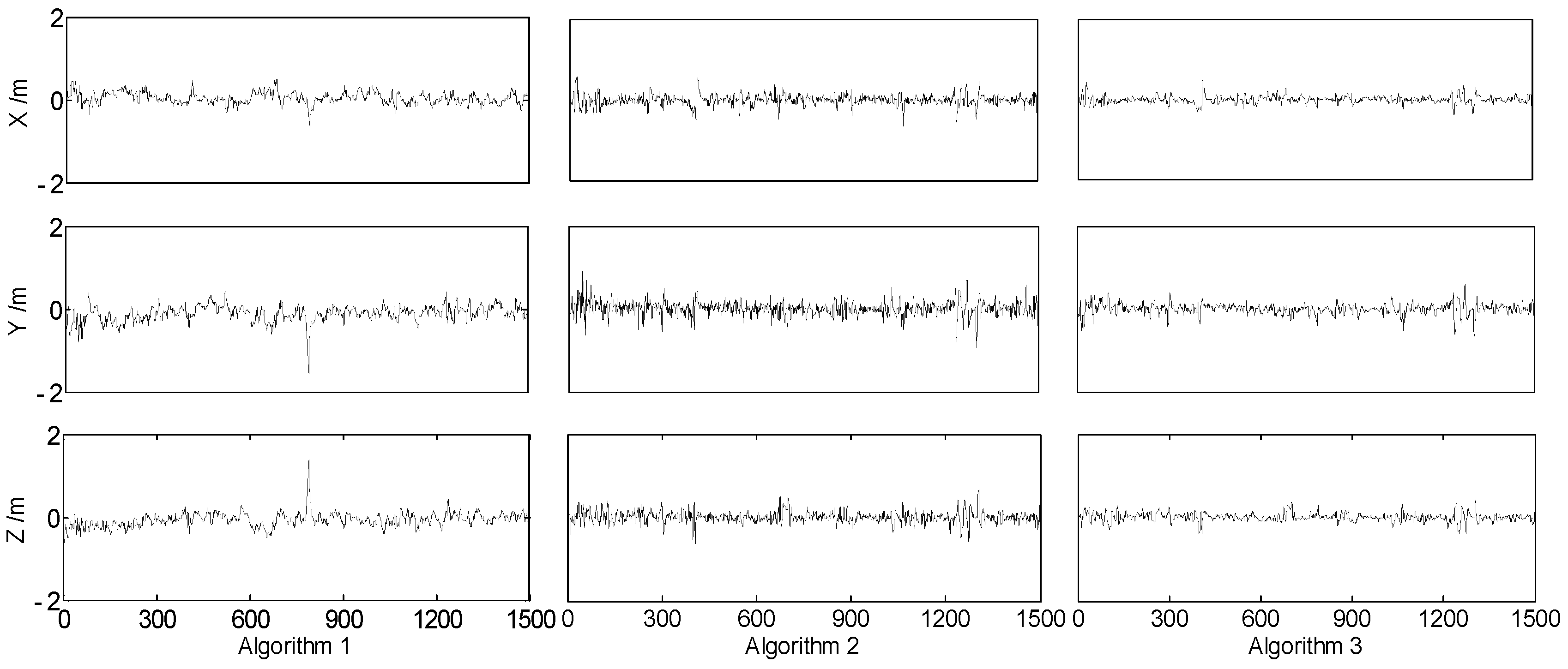
• Algorithm 1: the conventional cubature Kalman filter algorithm (marked as CKF);
• Algorithm 2: the nonlinear H∞ filter algorithm (marked as HF);
• Algorithm 3: the weighted-multiple-criteria-based filter algorithm (λ = 0.5, marked as MCF-0.5).

The GNSS position and velocity measurement errors are plotted in Figure 2 and Figure 3, respectively.

The differences between the referential solution and those of Algorithms 1 to 3 are calculated as errors to compare the performance of different algorithms. Therefore, the position errors were calculated and are plotted in Figure 4.

It is concluded from Figure 2, Figure 3 and Figure 4 that the GNSS measurement errors may affect the measurement input of the integrated systems and then affect the performance of the filtering. As demonstrated in Figure 4, the performance of these three algorithms is stable, and the position errors are relatively small at most epochs. When the land vehicle moves over the speed bumps, disturbances or outlying measurements may occur, and this may finally affect the performance of the filtering. Algorithm 1 exhibits some continuous apparent fluctuations, and these fluctuations may result from the GNSS measurement errors and the outlying measurements, indicating that the robustness of the cubature Kalman filter should be further enhanced. In comparison to the conventional cubature Kalman filter, the nonlinear H∞ filter performs better during these fluctuant epochs, demonstrating its robustness to uncertain disturbances. Nevertheless, some redundant errors are introduced into the solution at certain normal epochs with the H∞ filter due to parameter estimation by minimizing estimation error in worst-case scenarios. Fortunately, these redundant errors are not significantly larger than normal errors and occur at scattered epochs. In contrast to the previous two algorithms depicted in Figure 4, Algorithm 3 shows more stable error curves, with abnormal errors found only at a few epochs. This indicates a decrease in the number of abnormal errors with Algorithm 3. By integrating the advantages of both the cubature Kalman filter and the H∞ filter, the error amplitudes of the proposed algorithm are smaller than those of the previous two algorithms. In practical applications within positioning and navigation fields, not only the position but also the velocity and attitude of moving carriers are essential parameters. Therefore, RMS (root mean square) errors and SD (standard deviation) of these parameters were utilized to evaluate the different algorithms. The results for these parameters from the different algorithms have been calculated and organized in

Table 2. RMS and SD values of different algorithms. In this table, the RMS of each main parameter for the land vehicle with the above three algorithms is provided, and the SD of each parameter is calculated to examine the dispersion degree of the errors.

Algorithm	Index	Px (cm)	PY (cm)	Vx (cm/s)	VY (cm/s)	Pitch (°)	Yaw (°)
CKF	RMS	3.26	3.86	0.79	1.03	0.12	0.45
HF		2.72	3.36	0.53	0.81	0.10	0.37
MCF-0.5		2.37	3.02	0.30	0.51	0.09	0.29
CKF	SD	3.26	3.84	0.78	1.02	0.12	0.30
HF		2.71	3.40	0.53	0.80	0.10	0.32
MCF-0.5		2.36	2.98	0.30	0.51	0.09	0.25

.

In Table 2, the RMS values of the HF algorithm are smaller than those of the conventional CKF algorithm, indicating an improved precision of position and velocity with the HF algorithm. In loosely coupled GNSS/INS integrated navigation systems, only position and velocity information are input into the systems as measurements for filtering, while the state parameters of the INS are estimated and modified through a closed-loop feedback process. As a result, the precision of estimated attitude parameters is also improved. Compared to the conventional CKF and HF algorithms, the MCF-0.5 algorithm shows even smaller RMS values, further improving filtering performance. The standard deviation reflects the dataset dispersion. In terms of standard deviations, different algorithms show similar trends to RMS values, indicating relatively concentrated error values and improved filtering stability with the proposed algorithm. Compared to the conventional CKF algorithm, the precision of the position, the velocity, and the attitude achieved with the proposed algorithm for the land vehicle are improved by about 24%, 48%, and 35%, respectively.

Group 2:

• Algorithm 4: the weighted-multiple-criteria-based filter algorithm (λ = 0.2, marked as MCF-0.2);
• Algorithm 5: the weighted-multiple-criteria-based filter algorithm (λ = 0.4, marked as MCF-0.4);
• Algorithm 6: the weighted-multiple-criteria-based filter algorithm (λ = 0.6, marked as MCF-0.6);
• Algorithm 7: the weighted-multiple-criteria-based filter algorithm (λ = 0.8, marked as MCF-0.8);

In this group, the value of λ was set to 0.2, 0.4, 0.6, and 0.8 to examine the performance of the proposed algorithm with different weight adjustment factors. Then, four algorithms were performed and the errors of the position are demonstrated in Figure 5.

Comparing the error curves in Figure 5, it was found that the overall performance of these four algorithms is similar. However, there are still obvious differences at some epochs, and several of these obvious differences are marked with red ellipses. Compared with Algorithm 4, the amplitudes of the position errors in Algorithm 5 seem slightly smaller. As the value of the weight adjustment factor λ increases, the amplitudes of the position errors tend to increase gradually. When the weight adjustment factor λ increases, the weight of M increases, and the filtering is performed under the criterion M at more epochs. Thus, the ability of the filtering to deal with the abnormal observations and uncertainty errors is weakened, and the position error is likely to expand. However, when the value of λ decreases, the weight of J increases, and the redundant error may be brought into the filtering and the performance may become inferior. Therefore, the influence of differences on the final performance of the filtering is determined by multiple aspects in practical applications. The RMS errors and the SD of the position, the velocity, and the attitude with different values of λ were also calculated. These indexes for the different algorithms are listed in

Table 3. RMS and SD values of different algorithms. Similar to Table 2, both the RMS and SD indexes are calculated to examine the precision and the dispersion degree with different algorithms.

Algorithm	Index	Px (cm)	PY (cm)	Vx (cm/s)	VY (cm/s)	Pitch (°)	Yaw (°)
MCF-0.2	RMS	2.53	3.19	0.25	0.43	0.09	0.36
MCF-0.4		2.41	3.03	0.27	0.46	0.09	0.32
MCF-0.5		2.37	3.02	0.30	0.51	0.09	0.29
MCF-0.6		2.40	3.07	0.39	0.66	0.10	0.26
MCF-0.8		2.66	3.35	0.46	0.72	0.10	0.22
MCF-0.2	SD	2.48	3.13	0.22	0.38	0.08	0.36
MCF-0.4		2.40	2.98	0.28	0.46	0.09	0.29
MCF-0.5		2.36	2.98	0.30	0.51	0.09	0.25
MCF-0.6		2.39	3.06	0.45	0.60	0.10	0.24
MCF-0.8		2.62	3.21	0.49	0.75	0.10	0.20

.

In Table 3, the RMS and SD values of different errors are calculated with different values of λ. Concerning the position errors, the values of RMS become smaller and then bigger as the value of λ increases. When the value of λ is about 0.5, the value of RMS is the smallest. This indicates that in this experiment, the suitable value of λ is about 0.5 to achieve a relatively high precision of the position. In terms of the velocity errors, the values of RMS become bigger as λ increases. For the errors of position and velocity, the trend of value-changing is the same in the X, Y, and Z directions. However, the errors of pitch become bigger and those of the yaw become smaller as the value of λ increases. Since the errors of pitch and yaw change in different ways, a suitable weight adjustment factor λ should be chosen to guarantee the precision of the attitudes in practical applications. Overall, the RMS values of the weighted-multiple-criteria-based algorithms are smaller than those of the CKF or HF algorithms. Comparing the values of RMS and SD, it was found that they manifest a similar tendency, and this similar tendency also depicts the relations between the performance of different algorithms and the solution of the filtering. In other words, the precision and stability of the filtering are improved further with the weighted-multiple-criteria-based algorithms.

Group 3:

• Algorithm 1: the conventional cubature Kalman filter algorithm (marked as CKF);
• Algorithm 2: the nonlinear H∞ filter algorithm (marked as HF);
• Algorithm 3: the weighted-multiple-criteria-based filter algorithm (λ = 0.5, marked as MCF-0.5).

This group is designed to test the proposed algorithm with data from diverse urban environments. The value of λ is 0.5, since it performed better in Group 1. The position errors were calculated and are plotted in Figure 6.

Compared with the dataset in Group 1, this new dataset contains more disturbances and outliers, and this can be demonstrated from the amplitudes of the error curves in Figure 6. From Figure 6, it is indicated that the diverse urban environment, such as water, the urban canyon effect, and other uncertain factors, can significantly affect the GNSS signal. Throughout these three algorithms, the position errors are stable, except for some special epochs. Algorithm 1 still exhibits some continuous, apparent fluctuations. Compared with Algorithm 1, the error curve of Algorithm 2 looks more stable, but it still brings some redundant errors at certain normal epochs, and this is because too many outliers will affect the performance of the H∞ filter algorithm. Similar to the performance in Group 1, the error amplitudes of the proposed algorithm are smaller than those of Algorithms 1 and 2.

5. Conclusions

In the data fusion of GNSS/INS integrated navigation systems, most current filtering algorithms are proposed by minimizing the mean squared error, which may limit the potential for performance improvement. A different approach was proposed in this paper to enhance filtering performance by incorporating multiple criteria and introducing a factor to adjust the weights of different criteria. Then the proposed algorithm was tested using actual data collected from GNSS/INS integrated navigation systems. The detailed conclusions drawn from the experiments in this paper are as follows:

(1)

The experiments in this paper demonstrate that the H∞ filter manifests superior robustness and precision than the cubature Kalman filter in GNSS/INS integrated navigation systems, but sometimes the H∞ filter may introduce some redundant errors.

(2)

By integrating the strengths of different filtering algorithms, the proposed weighted-multiple-criteria-based filtering algorithm with a weight adjustment factor outperforms conventional algorithms based on a single criterion.

(3)

Different weight adjustment factors can lead to varying filtering performances. Therefore, selecting an appropriate weight adjustment factor is crucial for achieving precise and stable filtering solutions.

(4)

A series of data fusion methods with multiple criteria can be constructed with different criteria and different adjustment factors.

References

- Bos, M.S.; Fernandes, R.; Williams, S.; Bastos, L. Fast error analysis of continuous GNSS observations with missing data. J. Geod. 2013, 87, 351–360. [Google Scholar] [CrossRef]
- Tang, C.; Shi, H.; Zhang, L. Geomagnetic matching cooperative positioning method for unmanned boat cluster based on factor graph. Ocean Eng. 2024, 296, 116901. [Google Scholar] [CrossRef]
- Yu, Z.; Zhang, Q.; Zhang, S.; Zheng, N.; Liu, K. A state-domain robust autonomous integrity monitoring with an extrapolation method for single receiver positioning in the presence of slowly growing fault. Satell. Navig. 2023, 4, 20. [Google Scholar] [CrossRef]
- Godha, S.; Cannon, M.E. GPS/MEMS INS integrated system for navigation in urban areas. GPS Solut. 2007, 11, 193–203. [Google Scholar] [CrossRef]
- Cui, B.; Chen, X.; Tang, X. Improved cubature Kalman filter for GNSS/INS based on transformation of posterior sigma-points error. IEEE Trans. Signal Process. 2017, 65, 2975–2987. [Google Scholar] [CrossRef]
- Jiang, W.; Liu, D.; Cai, B.; Rizos, C.; ShangGuan, W. A fault-tolerant tightly coupled GNSS/INS/OVS integration vehicle navigation system based on an FDP algorithm. IEEE Trans. Veh. Technol. 2019, 68, 6365–6378. [Google Scholar] [CrossRef]
- Wang, W.; Dong, S.; Wu, W.; Guo, D.; Wang, X.; Song, H. Combining TWSTFT and GPS PPP using a Kalman filter. GPS Solut. 2021, 25, 1–12. [Google Scholar] [CrossRef]
- Kim, D.; Lee, J. Kalman-filter-based integrity evaluation considering fault duration: Application to GNSS-based attitude determination. GPS Solut. 2022, 26, 1–13. [Google Scholar] [CrossRef]
- Marković, L.; Kovač, M.; Milijas, R.; Car, M.; Bogdan, S. Error state extended Kalman filter multi-sensor fusion for unmanned aerial vehicle localization in GPS and magnetometer denied indoor environments. In Proceedings of the 2022 International Conference on Unmanned Aircraft Systems (ICUAS), Dubrovnik, Croatia, 21–24 July 2022; IEEE: Piscataway, NJ, USA; pp. 184–190. [Google Scholar]
- Impraimakis, M.; Smyth, A.W. An unscented Kalman filter method for real time input-parameter-state estimation. Mech. Syst. Signal Process. 2022, 162, 108026. [Google Scholar] [CrossRef]
- Arasaratnam, I.; Haykin, S. Cubature kalman filters. IEEE Trans. Autom. Control. 2009, 54, 1254–1269. [Google Scholar] [CrossRef]
- Arasaratnam, I.; Haykin, S.; Hurd, T.R. Cubature Kalman filtering for continuous-discrete systems: Theory and simulations. IEEE Trans. Signal Process. 2010, 4977–4993. [Google Scholar] [CrossRef]
- Zhao, Y. Performance evaluation of cubature Kalman filter in a GPS/IMU tightly-coupled navigation system. Signal Process. 2016, 119, 67–79. [Google Scholar] [CrossRef]
- Chang, G. Robust Kalman filtering based on Mahalanobis distance as outlier judging criterion. J. Geod. 2014, 88, 391–401. [Google Scholar] [CrossRef]
- Yang, Y. Adaptive Navigation and Kinematic Positioning; Surveying and Mapping Press: Beijing, China, 2006. [Google Scholar]
- Mohamed, A.H.; Schwarz, K.P. Adaptive Kalman filtering for INS/GPS. J. Geod. 1999, 73, 193–203. [Google Scholar] [CrossRef]
- Wang, Y.; Liu, J.; Wang, J.; Zeng, Q.; Shen, X.; Zhang, Y. Micro aerial vehicle navigation with visual-inertial integration aided by structured light. J. Navig. 2020, 73, 16–36. [Google Scholar] [CrossRef]
- Xia, Q.; Sun, Y.; Zhou, C. An optimal adaptive algorithm for fading Kalman filter and its application. Acta Autom. Sin. 1990, 16, 210–216. [Google Scholar]
- Yang, Y.; Ren, X.; Xu, Y. Main progress of adaptively robust filter with applications in navigation. J. Navig. Position 2013, 1, 9–15. [Google Scholar]
- Almas, M.A.; Sharma, K. A two stage mean and iterative median filter approach for image denoising. Int. J. Adv. Sci. Technol. 2020, 29, 5355–5361. [Google Scholar]
- Xu, P. Sign-constrained robust least squares, subjective breakdown point and the effect of weights of observations on robustness. J. Geod. 2005, 79, 146–159. [Google Scholar] [CrossRef]
- Chang, L.; Li, K.; Hu, B. Huber’s M-estimation-based process uncertainty robust filter for integrated INS/GPS. IEEE Sens. J. 2015, 15, 3367–3374. [Google Scholar]
- Rigatos, G.; Siano, P.; Wira, P.; Busawon, K.; Binns, R. A nonlinear H-infinity control approach for autonomous truck and trailer systems. Unmanned Syst. 2020, 8, 49–69. [Google Scholar] [CrossRef]
- Yang, Y.; He, H.; Xu, G. Adaptively robust filtering for kinematic. J. Geod. 2001, 75, 109–116. [Google Scholar] [CrossRef]
- Chandra, K.P.B.; Gu, D.W.; Postlethwaite, I. Fusion of an extended h∞ filter and cubature Kalman filter. IFAC Proc. Vol. 2011, 44, 9091–9096. [Google Scholar] [CrossRef]
- Juneja, A.; Juneja, S.; Bali, V.; Mahajan, S. Multi-criterion decision making for wireless communication technologies adoption in IoT. Int. J. Syst. Dyn. Appl. 2021, 10, 1–15. [Google Scholar] [CrossRef]
- Apkarian, P.; Noll, D.; Rondepierre, A. Mixed H2/H∞ control via nonsmooth optimization. In Proceedings of the 48h IEEE Conference on Decision and Control (CDC) Held Jointly with 2009 28th Chinese Control Conference, Shanghai, China, 15–18 December 2009; pp. 6460–6465. [Google Scholar]
- Chen, Y.; Yuan, J. An improved robust H∞ multiple fading fault-tolerant filtering algorithm for INS/GPS integrated navigation. J. Astronaut. 2009, 30, 930–936. [Google Scholar]
- Zhang, Q.; Meng, X.; Zhang, S.; Wang, Y. Singular value decomposition-based robust cubature Kalman filtering for an integrated GPS/SINS navigation system. J. Navig. 2015, 68, 549–562. [Google Scholar] [CrossRef]