Analysis of Nearshore Near-Inertial Oscillations Using Numerical Simulation with Data Assimilation in the Pearl River Estuary of the South China Sea

Abstract

The High-Frequency (HF) radar network has become an effective method for detecting coastal currents. In this study, we confirmed the effectiveness of the HF radar measurements by comparing with the Acoustic Doppler Current Profiler (ADCP) and explore the possibility of assimilating radar data into a regional coastal ocean model. A regional high-resolution model with resolution of 10 m was first built in the Pearl River Estuary (PRE). However, analysis of the Hovmöller diagrams from the model simulations in this study indicated a significant deficiency in representing Near-Inertial Oscillations (NIOs) in the PRE, particularly in the east–west direction, despite including wind fields in the input data, during the week from 3 to 8 August 2022. To overcome the model deficiency, we conducted a set of assimilation experiments and performed sensitivity analyses. The results of sensitivity experiments indicate that the model exhibits a sufficient capacity to replicate NIOs after assimilation, lasting approximately 5–6 days. To further analyze the reasons for the decay in the magnitude of the NIOs, data from the three ADCP stations were compared with model results by applying the momentum equation. The assimilated vertical diffusion term outperforms the unassimilated model in representing NIOs. These findings highlight the importance of the vertical diffusion term for simulating NIOs and the data assimilation in improving the model’s representation of physical processes.

1. Introduction

Near-inertial motion represents an oscillatory component of the ocean’s response to wind forcing, influenced by the Earth’s rotation and the production of depth-veering currents relative to the wind direction, initially derived by Ekman [1]. It is characterized by near-circular horizontal currents rotating clockwise in the Northern Hemisphere and counterclockwise in the Southern Hemisphere, primarily occurs in the upper ocean [2,3]. This motion exhibits transience, arising from significant wind shifts and subsequently decaying exponentially when the winds subside, indicating its sensitivity to wind conditions and non-persistent nature [4,5,6,7].

Near-inertial oscillations (NIOs) are a significant component of oceanic variability, characterized by motions that are closely tied to the local inertial frequency [8,9,10,11,12]. These oscillations play a crucial role in the mixing and transport processes in the ocean, influencing phenomena ranging from nutrient distribution to climate dynamics [13]. Accurate simulation of NIOs is essential for understanding and predicting oceanic behaviour, particularly in coastal regions where these oscillations can have pronounced effects [14,15,16]. The Pearl River Estuary (PRE) in southern Guangdong Province, China, has been a region of extensive studies regarding NIOs (for instance, Pan et al. [17] and Chen et al. [18]). Due to its unique topography, connecting to the Delta River network and the South China Sea (SCS), and the presence of multiple major river inlets, comprehending the circulation characteristics and effects of NIOs in the PRE is essential for early disaster warning and mitigation efforts in the region.

The Acoustic Doppler Current Profiler (ADCP) has been in development for decades and is capable of measuring the current velocity at a specific point [19,20,21]. However, being limited to a single-point measurement method, it cannot comprehensively capture the dynamics of the current. High-Frequency (HF) radar can address this limitation. It has been utilized for many years in observing ocean circulation. Employing electromagnetic wave inversion based on the Bragg scattering principle enables the acquisition of data related to wind, waves, and surface currents in the ocean. Over time, the accuracy of this data has been increasingly recognized [22,23,24,25,26,27,28,29]. For instance, HF radar can describe complex cross-shore structures of Bodega Bay in northern California, USA, revealing its main feature: the weak poleward currents over the inner shelf [30]. In June 2010, an analysis of surface currents obtained through an HF radar confirmed that the diurnal oscillations in the northeastern Gulf of Mexico were primarily attributed to wind-forced inertial oscillations [31]. Data from the HF radar indicated that surface currents were relatively weak in coastal areas during the passage of Hurricane Arthur in 2014 but increased in strength as the hurricane moved offshore [32]. Various scholars have investigated the detection of NIOs in the ocean by using HF radars. Victor et al. showed that NIO surface signatures are easily captured by HF radars in the northwestern Mediterranean [33]. In a 1996 field program, an HF radar provided the temporal evolution of NIO motion on New Jersey’s inner shelf [34]. Rubio et al. utilized HF radar surface current data to map the variability associated with the near-inertial waves in the SE Bay of Biscay in 2009 [35]. Yukiharu Hisaki and Tatsunori Naruke estimated the horizontal variability of NIO during a typhoon passage using HF radar observations [36]. These examples illustrate the feasibility of using HF radars to observe NIOs phenomena in the ocean [37].

Assimilating HF radar data into numerical ocean models offers a promising avenue for enhancing the accuracy of NIO simulations. By integrating real-time observational data with model predictions, data assimilation techniques can correct model discrepancies and reduce uncertainties. FVCOM, developed by Chen et al. [38], is a community ocean model with a prognostic, unstructured-grid, finite-volume, free-surface, three-dimensional (3-D) primitive equation. Nudging, a commonly employed data assimilation technique, merges model predictions of physical variables with observed data, incorporating predetermined statistical assumption regarding model and observational errors. Previous studies have demonstrated the feasibility of the nudging method [39,40,41]. The first successful application of nudging to ocean data assimilation appeared in 1992 in a study that assimilated sea surface height data derived from satellite measurements into a quasi-geostrophic layered model [39]. Since then, this method has been successfully applied to solve a variety of ocean numerical problems. Chen et al. (2013) used nudging data assimilation to estimate model boundary conditions [40]. Li et al. (2012) used nudging data assimilation to address the model downscaling problem [41]. The appeal of this approach for nudging data problems lies in its simplicity of implementation in complex numerical models, low computational power requirements, and the temporal smoothness of the solution [42]. Studies have explored the feasibility of assimilating HF radar currents into numerical models. Shulman et al. developed a high-resolution data assimilation ocean model for the Monterey Bay area, showcasing the model’s capability to track major mesoscale ocean features [43]. James et al. (1998) used the nudging assimilation scheme to find that the model surface currents obviously tend to the fundamental characteristics of the observed field of Doppler radar currents [44]. HF radar data assimilation has been shown to reduce spatial and temporal shifts, leading to a significant improvement in the correlation between the model and observed subsurface currents [45].

Previous studies have demonstrated the effectiveness of data assimilation of HF radar velocity observations in correcting the phase and amplitude of inertial oscillations [46], which is the primary focus of this paper. However, these studies often concentrate on the effect of typhoons on NIOs or the availability of HF radar data. Meanwhile, there are fewer studies specifically addressing the assimilation of HF radar data, especially in the PRE region. Moreover, our team independently established the HF radar network in the PRE, which serves as the primary technical tool for ocean observation in the region. In this study, 2-D near-surface current data obtained from HF radar measurements conducted between 17 July and 17 August 2022, in conjunction with a numerical model to investigate the circulation characteristics and propagation of NIOs in the generalized context of the PRE region. To prove the credibility of the radar data, we aim to compare the current feature between the model and HF radar data. Subsequently, we identified that the model alone inadequately represents NIOs, prompting us to implement nudging assimilation by incorporating HF radar data. The objective is to improve the model’s performance by assimilating the HF radar data and thereby enhance the credibility of the model results.

This paper is structured as follows: Section 2 presents an overview of the data, model, and research methods. Section 3 presents an evaluation of the radar data. Section 4 encompasses an EOF analysis of the data, sensitivity experiments involving the model, and an analysis of vertical diffusion item within NIOs. Section 4 and Section 5 present the discussion and conclusions of the paper.

2. Data, Model and Methods

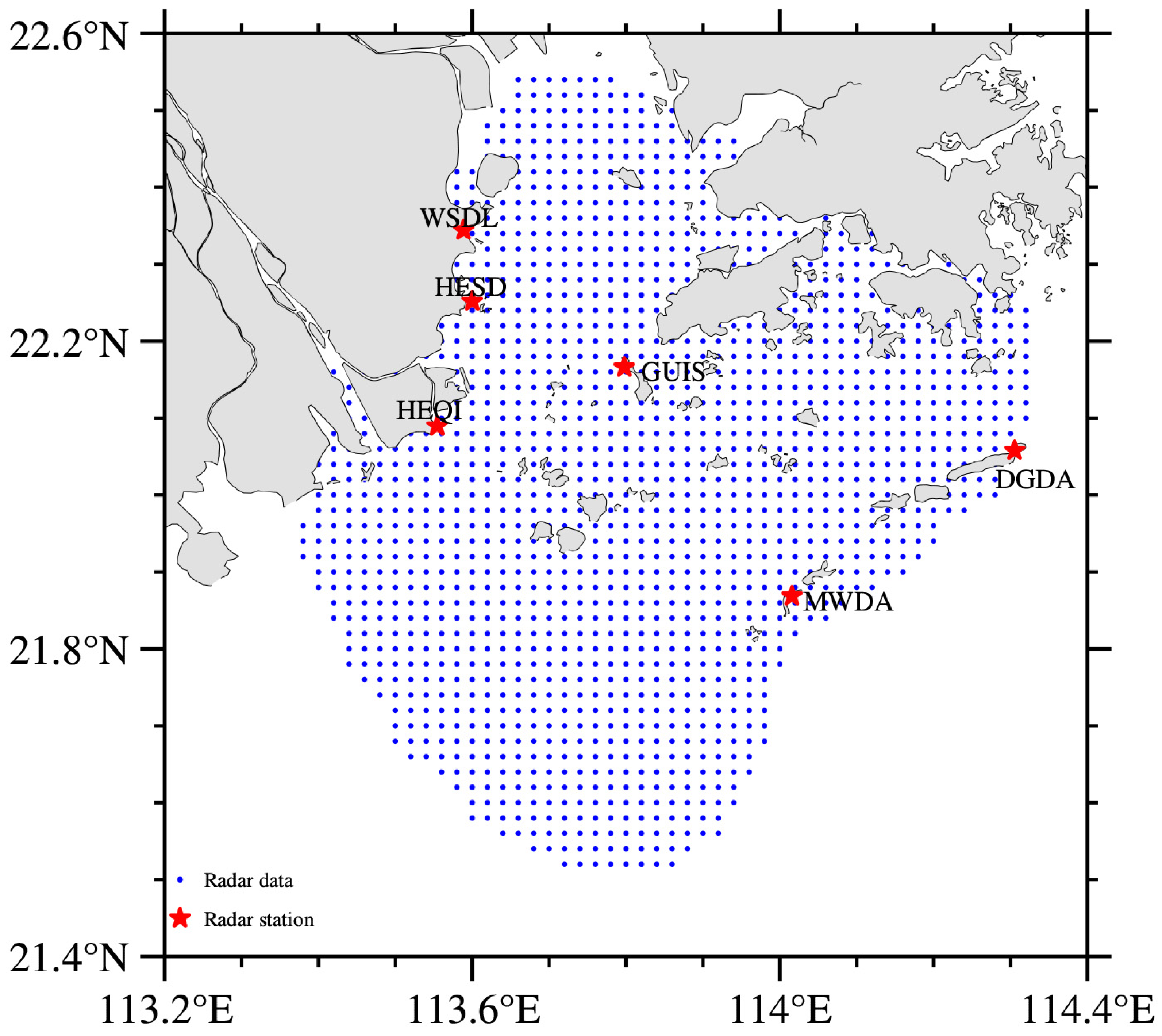
2.1. High-Frequency Radar Data

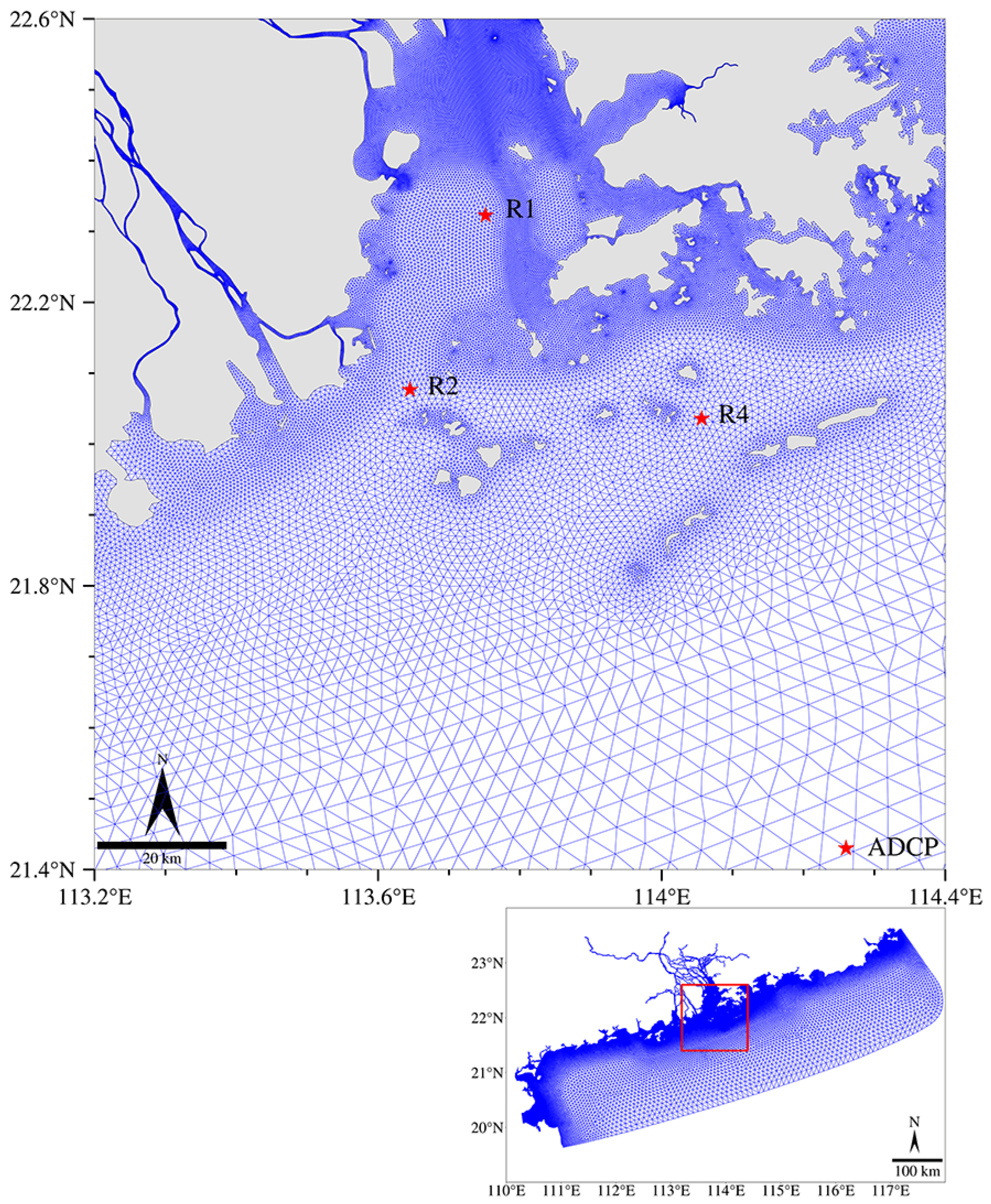
In several studies, including those by Teague et al. [22] and CROMBIE [24], the principles of HF radar for surface current measurements have been extensively elucidated. HF radar operates by emitting high-frequency radio signals within the 5–25 MHz range, which interact with the ocean surface and are backscattered. This interaction leads to the formation of Bragg scatter, where ocean gravity waves with half the transmitted wavelength produce a pronounced peak in the returned energy spectrum. The difference between the anticipated and observed Doppler shift of this peak is then harnessed to compute the component of the surface current, either moving toward or away from the radar station.

In this study, we acquired hourly 2-D near-surface current velocities using six shore-based OSMAR-S100 HF radars (13–16 MHz) located at stations GUIS, HEQI, HESD, MWDA, WSDL, and DGDA. These radar systems are diligently managed and operated by Wuhan University as integral components of the Greater Bay Area (GBA) research initiative. The radar network extends its coverage over approximately 150 km along the coastal region proximate to the PRE. The precision of surface current measurements obtained through HF radar is subject to variability and influenced by various factors, including the signal-to-noise ratio, sea state conditions linked to wind speed and direction, and potential radar frequency interference [47,48,49]. The data consists of information obtained from 17 July to 17 August 2022, covering a substantial detection area (113.4°E–114.3°E, 21.5°N–22.6°N), totaling over 10,000 km². This dataset produced “total vectors,” which represent hourly u (east–west) and v (north–south) components of near-surface current velocities, and these values were interpolated onto a 5 km Cartesian grid, as illustrated in Figure 1.

2.2. Mooring Data

Within the context of the HF Surface Wave Radar Experiment, three moorings (R1, R2, and R4, arranged from north to south, as shown in Figure 2), were deployed in the PRE from July to August 2022. These moorings were equipped with Teledyne RD Instruments Workhorse II Sentinel ADCP systems, operating at 600 K or 1200 K frequencies, enabling the measurement of upper ocean currents. Data were collected at 20 min intervals, with vertical resolutions of 1 m or 0.5 m. The blank distances calculated from the ADCP were 1.61 m (R1), 2.11 m (R2), and 2.12 m (R4). For our study, velocities from the nearest cell (Bin) to the surface based on the water depth were selected for comparison. The effective vertical velocity ranges were 1.61–6.61 m, 2.11–8.11 m, and 2.12–30.12 m for moorings R1, R2, and R4, respectively, as detailed in

Table 1. Information of the Workhorse II Sentinel ADCP.

Site	R1	R2	R4
Location	113.75°E, 22.32°N	113.65°E, 22.08°N	114.06°E, 22.04°N
Frequency	1200 kHz	600 kHz	600 kHz
Time interval	20 min
Top layer depth	1.61 m	2.11 m	2.12 m
Vertical resolution	0.5 m	1 m	1 m
Max profiling range	20 m	70 m	70 m
Standard sensors	Temperature, Tilt, Compass
Beam angle	20°

, providing further information on each mooring.

2.3. Model and Design of the Experiments

FVCOM is a numerical model based on an unstructured grid, offering the advantage of geometric flexibility to accommodate complex shorelines and bathymetry. Our mesh comprises 358,489 non-overlapping horizontal triangular cells and 214,428 nodes, with grid sizes ranging from 10 m to 10 km (Figure 2). Notably, the grid resolution smoothly transitions from 10 m to 2 km within the PRE region, which is the primary area of focus (Figure 2).

Topographical and bathymetric data in our model were derived from high-resolution survey data sourced from the Nautical Chart, supplemented by bed sweeping information furnished by CCCC (China Communications Construction Company), specifically the first Harbour Engineering Company Limited. The wind forcing data at 10 m above the ocean surface were acquired from the National Centers for Environmental Prediction (NCEP) Climate Forecast System Version 2 (CFSV2), serving as the primary wind driver in our study. The spatial coverage consists of 1.875 longitude × 1.915 latitude global grids (192 × 94), with a time interval of 6 h. It meets the requirements of the model and has been thoroughly validated previously [47,49]. The TPXO8 tidal model was employed to implement tidal influences at the lower open boundary. Additionally, we utilized the Tide Model Driver (TMD) to compute elevations along this boundary, encompassing eight major tidal constituents (M2, N2, S2, K2, K1, O1, P1, and Q1), thereby effectively simulate tidal currents in the vicinity of the PRE. The model took into account the river discharges of seven key rivers, namely, Tanjiang, Xijiang, Beijiang, Liuxi, Zengjiang, Hanjiang, and Dongjiang. For this purpose, daily flow data from the Shijiao, Gaoyao and Boluo stations during the dry season (November to April) from 2003 to 2007 were employed. These flow statistics were generously provided by the Guangdong Hydrological Bureau. Initial temperature and salinity were obtained from Simple Ocean Data Assimilation (SODA). The modelling simulation extended from April to September 2022, with the initial two months serving as the spin-up phase. The simulation interval for the remaining period corresponded to the time scales of the observed data. In the vertical direction, the model utilized a terrain tracking coordinate system that combined $\sigma$ and spherical coordinates, dividing the vertical domain into 20 layers with a high resolution up to 0.25 m. Zhu et al. [47] have verified the scientific validity of the model.

In our model runs, we implemented time steps of 1.0 s for the external mode and 5.0 s for the internal mode. The assimilation scheme in this study is a nudging scheme. The summarized settings of the three model experiments, denoted CTR, EXP1, and EXP2, are shown in

Table 2. Experimental design.

Experiment Name	Time	Wind	Tide	River Discharge	Assimilation	Assimilation Time	Assimilation Data
CTR	17 July to 17 August 2022	√	√	√
EXP1		√	√	√	√	17 July to 17 August 2022	radar
EXP2		√	√	√	√	17 July to 30 July 2022	radar

. Nudging involves assimilating model-predicted physical variables directly with observational data based on predefined statistical assumptions concerning model noise and observational data errors [50]. The governing equation for the nudging assimilation process is provided as follows:

$${\displaystyle \frac{∆{\alpha }_i}{∆t}}=F_i+G_{\alpha }{\displaystyle \frac{\sum _{i=1}^N{W}_i^2{\gamma }_i{\left({\alpha }_o-\widehat{\alpha }\right)}_i}{\sum _{i=1}^N{W}_i}}$$

(1)

In the context of this assimilation method, ${\alpha }_o$ represents observed values, $\widehat{\alpha }$ signifies model-predicted values, and ${\alpha }_i$ represents the chosen variable for assimilation. The term $F_i$ encompasses all components in the governing equation of ${\alpha }_i$ except the local temporal change. Furthermore, ${\gamma }_i$ denotes the data quality factor at the $i$th observational point, with values ranging from 0 to 1. $G_{\alpha }$ is a nudging factor that keeps the nudging term to be scaled by the slowest physical adjustment process ($G_{\alpha }=1/t\prime$, $t^{\prime }$ is the nudging timescale, unit: s). $W_i$ is a product of weight functions given as $W_i=w_{xy}\bullet w_{\sigma }{\bullet w}_t{\bullet w}_{\theta }$, where $w_{xy},w_{\sigma },w_t$ and $w_{\theta }$ are horizontal, vertical, temporal and directional weighting functions, respectively. The mathematical expressions of these functions are given as

$$w_{xy}=\left\{\begin{array}{cc}{\displaystyle \frac{R^2-r^2}{R^2+r^2}}& 0\le r\le R\\ 0& r>R\end{array}\right.$$

(2)

$$w_{\sigma }=\left\{\begin{array}{cc}1-{\displaystyle \frac{{\sigma }_{obs}-\sigma }{R_{\sigma }}}& \left|{\sigma }_{obs}\right.-\left.\sigma \right|\le R\\ 0& \left|{\sigma }_{obs}\right.-\left.\sigma \right|>R\end{array}\right.$$

(3)

$$w_t=\left\{\begin{array}{cc}1& \left|t\right.-\left.t_0\right|<T_w/2\\ {\displaystyle \frac{T_w-\left|t\right.-\left.t_0\right|}{T_w/2}}& T_w/2\le \left|t\right.-\left.t_0\right|\le T_w\\ 0& \left|t\right.-\left.t_0\right|>T_w\end{array}\right.$$

(4)

$$w_{\theta }={\displaystyle \frac{\left|\left|∆\right.\left.\theta \right|\right.-\left.0.5\pi \right|+c_1\pi }{(0.5+c_1)\pi }}$$

(5)

where $R$ is the search radius, $r$ is the distance from the location where the data exists, $R_{\sigma }$ is the vertical search range, $T_w$ is half of the assimilation time window, and $∆\theta$ is the directional difference between the local isobath and the computational point, with $c_1$ being a constant ranging from 0.05 to 0.5.

In control experiments (CTR), the model is not assimilated. EXP1 is a one month assimilation experiment conducted from 17 July 2022 to 17 August 2022, to evaluate the outcomes of assimilating HF radar data. To verify the assimilation duration of the nudging scheme, EXP2 was set to assimilate data from 17 July 2022 to 31 July 2022, without further assimilation from 1 August onward. Furthermore, to conduct a single-point analysis, three points corresponding to the ADCP were chosen to represent this region for a more comprehensive time series analysis (Figure 2).

2.4. Empirical Orthogonal Function (EOF) Analysis

Preisendorfer et al. [51] provided a comprehensive account of empirical orthogonal function (EOF) analysis, a widely employed method in atmospheric and oceanographic sciences. This technique enables the identification of spatial patterns of variability for specific variables and tracking their temporal evolution over time [52,53,54,55]. In this study, EOF analysis was utilized to compare radar with the model, aiming to characterize the current in the PRE region. The data for analysis is selected, preprocessed, and transformed into an anomaly form. In mathematical terms we can treat the array as a $2m\times n$ matrix as follows:

$$X=\left[\begin{array}{cccc}{u}_1\left(1\right)& u_1\left(2\right)& \cdots & u_1\left(n\right)\\ u_2\left(1\right)& u_2\left(2\right)& \cdots & u_2\left(n\right)\\ ⋮& ⋮& ⋮& ⋮\\ u_m\left(1\right)& u_m\left(2\right)& \cdots & u_m\left(n\right)\\ v_1\left(1\right)& v_1\left(2\right)& \cdots & v_1\left(n\right)\\ v_2\left(1\right)& v_2\left(2\right)& \cdots & v_2\left(n\right)\\ ⋮& ⋮& ⋮& ⋮\\ v_m\left(1\right)& v_m\left(2\right)& \cdots & v_m\left(n\right)\end{array}\right]$$

(6)

In this context, m represents the number of points, and n represents the number of time periods. With these data, the covariance matrix $S$ can also be written in the following way:

$$S={\displaystyle \frac{1}{n-1}}X{X}^T$$

(7)

The eigenvalues ($V$) and eigenvectors $(\Lambda$) of the square matrix $S$ are calculated, and both conditions are met:

$$S=V\times \Lambda$$

(8)

where $\Lambda$ is a $2m\times 2m$ diagonal matrix, that is:

$$\Lambda =\left[\begin{array}{cccc}{\lambda }_1& 0& \dots & 0\\ 0& {\lambda }_2& \dots & 0\\ \dots & \dots & \dots & \dots \\ 0& 0& \dots & {\lambda }_{2m}\end{array}\right]$$

(9)

Generally, the eigenvalues ($\lambda$) are arranged in descending order. Since the data matrix $X$ represents the observed values, $\lambda$ must be greater than or equal to 0. The eigenvector corresponding to each non-zero eigenvalue is called an EOF. Specifically, the eigenvector corresponding to ${\lambda }_k$ is the $k-th$ column of $V$: ${EOF}_k=V(:,k)$. According to this article, since velocity is a vector, the first mode is $u_1=V(:,1)$, $v_1=V(:,m+1)$. the second mode is $u_2=V(:,2)$, $v_2=V(:,m+2)$.

To accomplish this work, we introduced the EOF ellipse to compare two time series of radar and model current, which can aggregate the u-component velocity and v-component velocity.

$$X=\left[\begin{array}{cccc}{u}_1\left(1\right)& u_1\left(2\right)& \cdots & u_1\left(n\right)\\ v_1\left(1\right)& v_1\left(2\right)& \cdots & v_1\left(n\right)\end{array}\right]$$

(10)

Following this method, EOF analysis is employed to decompose the velocity matrix into first and second modes using a two-dimensional spatial vector:

$$\Lambda =\left[\begin{array}{cc}{\Lambda }_1\left(t\right)& {\Lambda }_2\left(t\right)\end{array}\right]$$

(11)

The ellipse was constructed with the major axis aligned with the first mode of eigenvalues, signifying the largest standard deviation of total velocities, while the minor axis corresponded to the second mode of eigenvalues. The orientation of the ellipse was calculated as follows:

$$\theta =arctan\left({\displaystyle \frac{{\Lambda }_2\left(t\right)}{{\Lambda }_1\left(t\right)}}\right)$$

(12)

${\Lambda }_1\left(t\right)$ and ${\Lambda }_2\left(t\right)$ are the first and second eigenvector modes, respectively. Additionally, this operation is sequentially performed on each site, ultimately calculating the EOF ellipse data for each site.

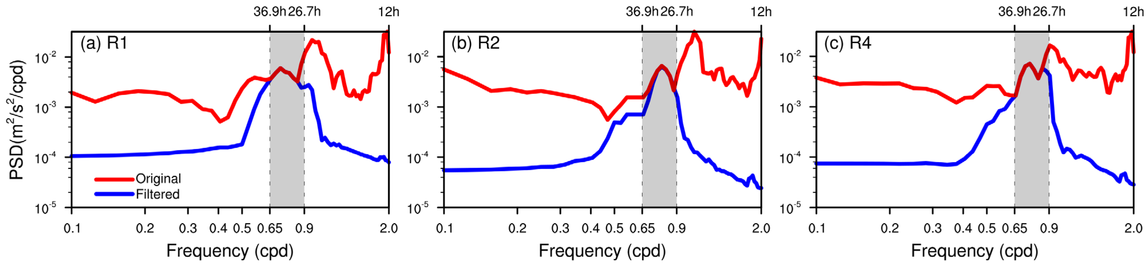
2.5. Filtering and Frequency Band Selection

This study primarily focuses on near-inertial oscillations within the PRE region. In this region, the frequency of diurnal tide closely approximates that of near-inertial, which are defined within the range of {0.9, 1.1}$f$ times the inertial frequency (where $f=2\mathsf{\Omega }\sin \phi$, with $\mathsf{\Omega }$ representing Earth’s angular velocity and $\phi$ denoting the latitude). Given the geographical context of our study in the PRE, the defined range for near-inertial frequency in this region falls within 0.65–0.9 cpd.

To further investigate the current in the near-inertial frequency, we processed the surface current time series using a two-step digital filtering procedure with MATLAB numerical routines. A two-step filtering approach was employed due to the relatively narrow frequency bands of interest, specifically the near-inertial range (0.65–0.9 cpd), which constituted only a fraction of the total bandwidth. In the first step, the entire dataset was filtered to isolate tidal components using the known diurnal tide frequency as a reference. Subsequently, the extracted data from this initial filtering underwent bandpass filtering within the near-inertial frequency band, facilitated by a fourth-order Butterworth filter in the second step. Figure 3 presents the comparison of filtering results at the three stations (R1, R2 and R4). The figure illustrates that, compared to the original data, the energy is stronger only in the near-inertial frequency range after filtering (blue line), and the processed data meets our analysis requirements for this band.

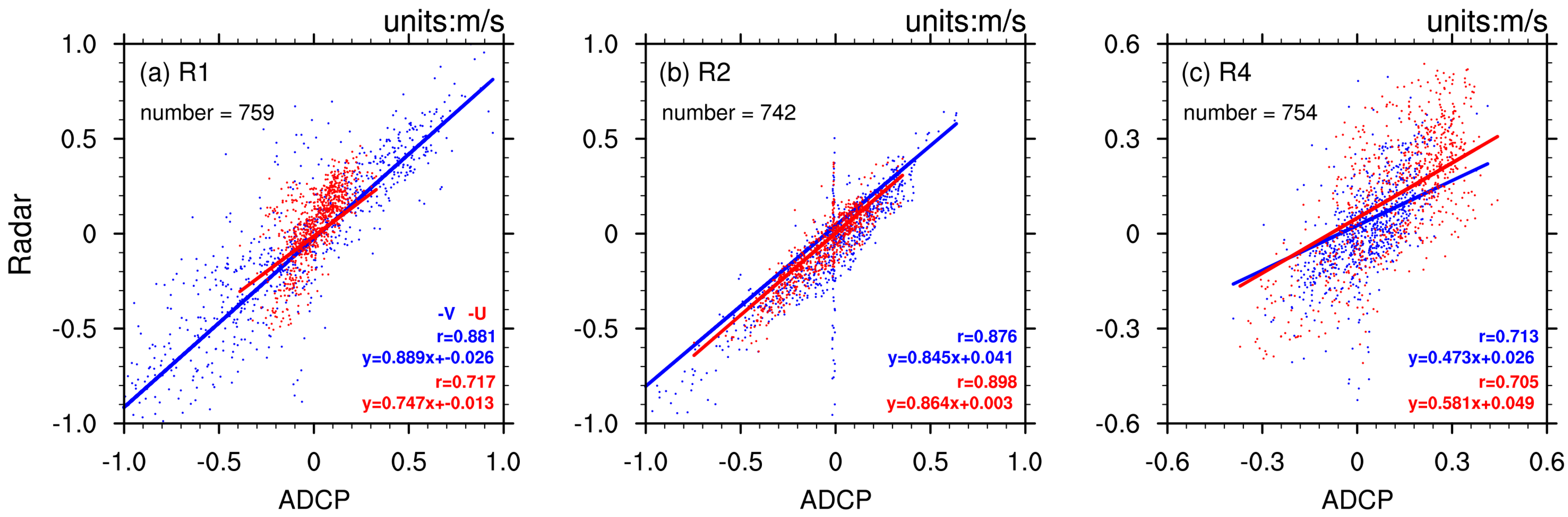
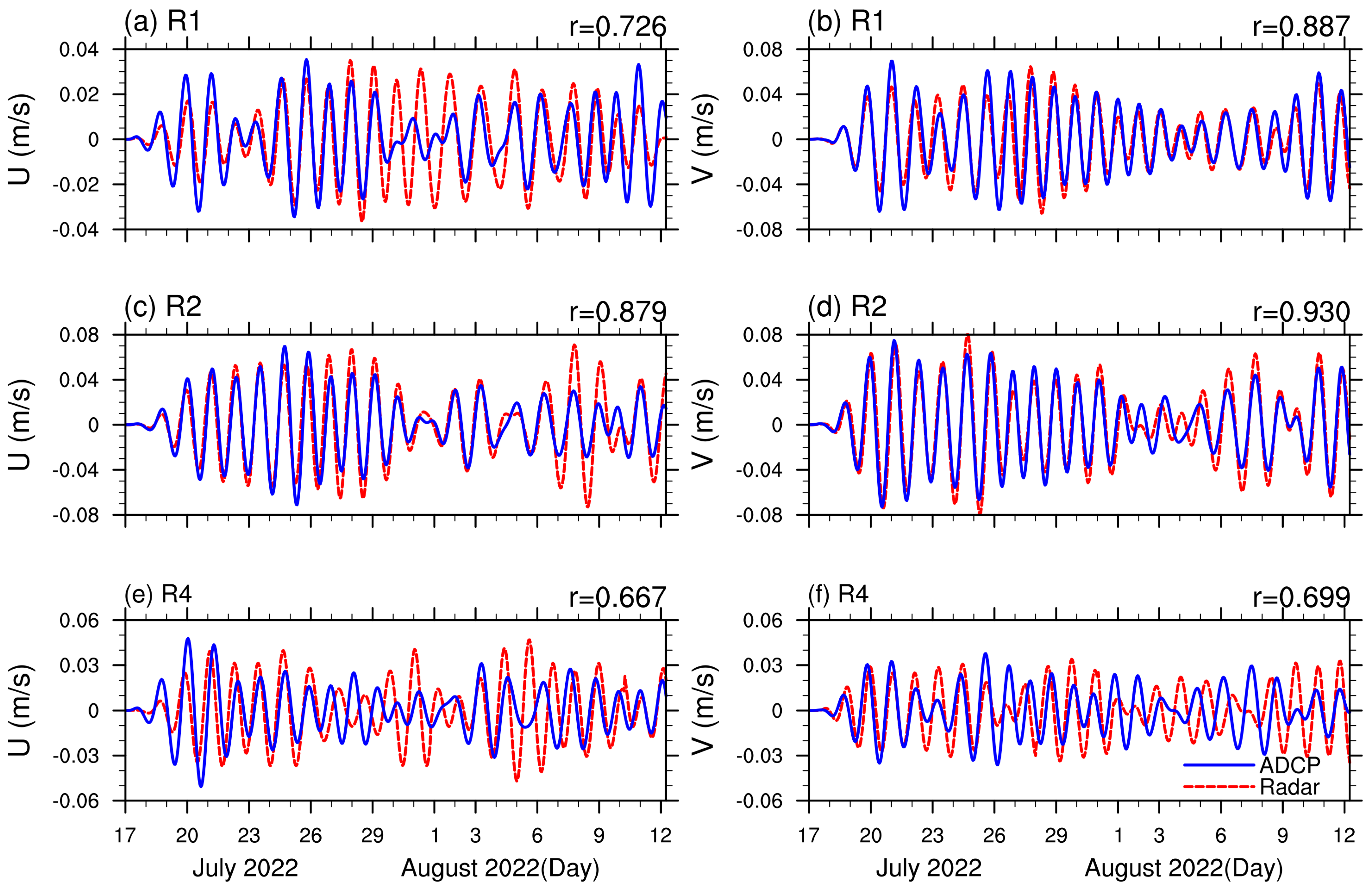
2.6. Evaluation of HF Radar Data

ADCPs have frequently been utilized as dependable instruments to assess the accuracy of HF radar detection [27,56]. To validate the data derived from HF radar, we compared the near-surface HF radar current measurements (approximately 1 m depth) with those obtained by ADCPs. This comparison was executed by aligning the latitude and longitude coordinates of the three ADCPs listed in Table 1 with the closest HF radar pixel points.

Figure 4 and Figure 5 compare the EOF ellipses and HF radar data of the three stations for one month, respectively. Data from the three ADCP stations and the corresponding radar data are used as two-dimensional data sets for EOF ellipse analysis. Figure 4 shows that the EOF ellipse data of the three stations all exhibit significant overlap, indicating that the current characteristics obtained by HF radar and ADCP are highly consistent.

Table 3. Statistics of the ADCP and HF radar EOF ellipses amplitudes (m/sec) and rotation (degrees).

EOF Ellipse		R1	R2	R4
major axis	ADCP	0.378	0.408	0.423
	HF radar	0.442	0.300	0.189
minor axis	ADCP	0.091	0.160	0.259
	HF radar	0.180	0.138	0.147
rotation	ADCP	86.962	53.427	177.822
	HF radar	83.006	65.006	165.611
RMSE		0.110	0.110	0.259

provides the specific values of the EOF ellipse, with RMSE used as a quantitative measure of the difference between HF radar and ADCP ellipses. The RMSE formula is:

$$RMSE=\sqrt{{\left(L{maj}_{radar}-L{maj}_{ADCP}\right)}^2+{\left(L{min}_{radar}-L{min}_{ADCP}\right)}^2}$$

(13)

Upon assessing the RMSE and differences in the major and minor axes, as well as the rotation of the two datasets, it becomes evident that the disparities are minimal, as indicated in Table 3, with the RMSE of the R1 and R2 stations is only 0.11 m/s. Particularly for the R2 site, the difference between the major and minor axes of its EOF ellipse is less than 0.1. Figure 5 further validates this comparison, indicating that the correlation of both data sets and ADCP data is very high. At station R2, the correlation coefficient between the two data sets are close to 0.9 and a slope close to 1 (Figure 5b), and for the other two stations, it is above 0.7. Both the EOF analysis and the data comparison analysis indicate that the data quality at the R4 site has declined (Figure 5c), possibly due to island barriers and the complex terrain and coastline in the area. Overall, the HF radar effectively captured the current variations observed by the ADCPs during this period.

Figure 6 compares the time series of near-inertial currents obtained using the procedure outlined in Section 2.5 at three stations. Although the correlation between the two data sets is lower than that of the ocean current, it remains high, with both exceeding 0.65. Notably, at the R2 station (Figure 6c,d), the correlation coefficient is close to 0.9, consistent with the findings of Figure 5. The performance of the near-inertial current in the u-component and the v-component is essentially the same. Therefore, the HF radar data are reliable for both ocean currents and near-inertial currents and can serve as candidate data for assimilation.

3. Results

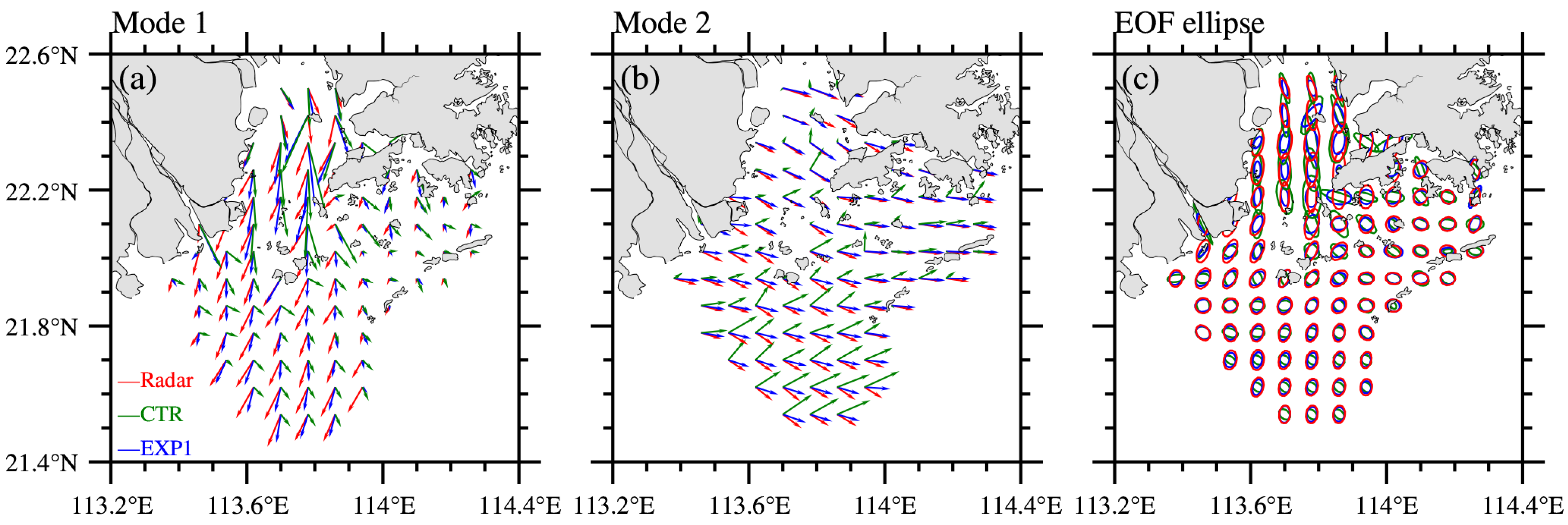
3.1. EOF Analysis of Model and Radar Data

Considering the pivotal role of NIOs in driving circulation within the PRE, the EOF ellipse can effectively capture the overall characteristics of these oscillations. Such analysis facilitates the identification and description of near-surface inertial oscillations, as elucidated by Gough et al. [31]. Our study commenced with an EOF analysis for the designated study area. The model data were obtained following the method described in Section 2.3 and analyzed after being matched with the longitude and latitude of the radar data. The comparison of the EOF ellipses, illustrated in Figure 7c, reveals good agreement between the HF radar (red) and the assimilated model (blue). The shapes of these ellipses indicate that the PRE can be divided into two circulation regions: the offshore region and the alongshore region. Along the coast, substantial variations are observed in the size and orientation of the EOF ellipses, characterized by a distinct south-to-north elongation. The complex coastline and the presence of islands are likely the primary factors contributing to these discrepancies. In contrast to the alongshore EOF ellipse, the offshore EOF ellipse is relatively smaller. This disparity may stem from the suppression or intensification of the u-component oscillation during this period, as opposed to variations in the v-component oscillations.

Within the latitude range of 21.5°N to 22.0°N, the impact of islands and coastlines diminishes markedly, resulting in a close overlap between the radar and model ellipses. It indicates a remarkable level of consistency between the currents obtained from HF radar measurements and those simulated by the model. In Figure 7a, the first mode of the EOF current analysis is displayed, revealing a consistent north–south predominant current within the PRE, regardless of the data source. The first mode accounts for over 50% of the variance. The second mode is also significant and indicates that the second major current in the PRE is characterized by an east–west direction. It is also observed that nudging assimilation can improve model quality, aligning it more closely with radar observations. This finding is consistent with the primary focus of our research in this article.

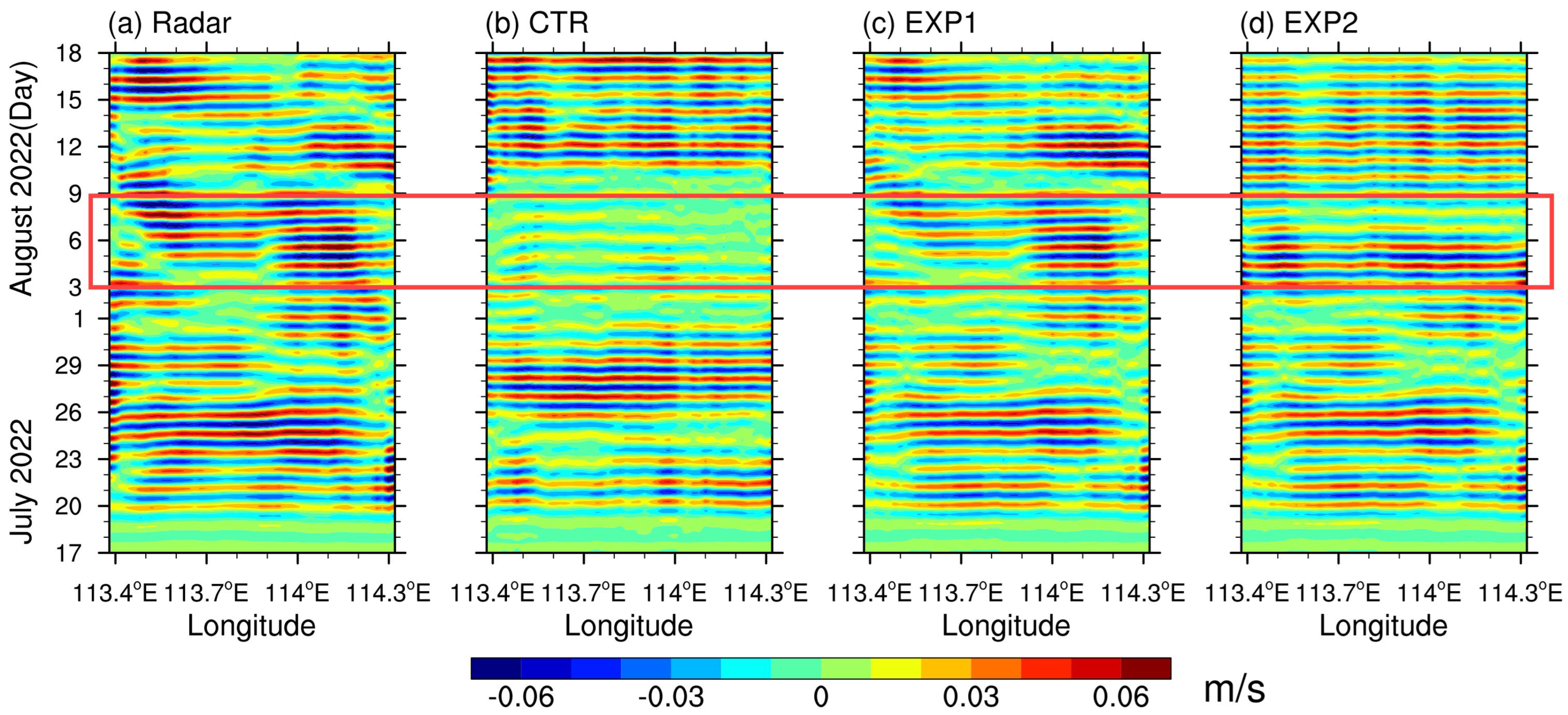
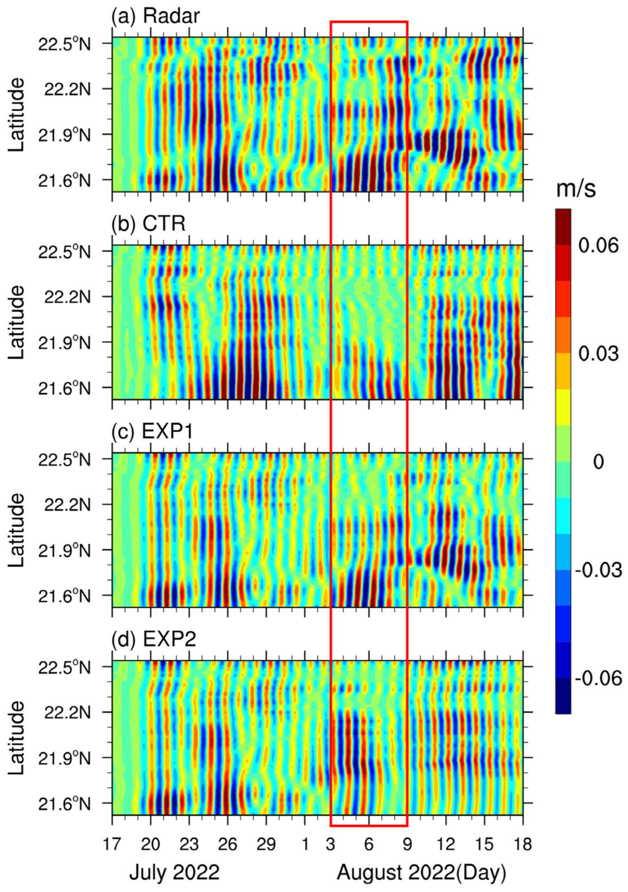
3.2. Sensitivity Experiments for Near-Inertial Oscillations Using FVCOM

Utilizing Hovmöller diagrams enables us to effectively discern oscillatory signal propagation and sudden spatiotemporal transitions, a valuable approach detailed by Gough et al. in 2016 [31]. A key characteristic of NIOs in the PRE is their large amplitude and spatially coherent motion. As discussed in Section 3.1, the EOF analysis shows that the model and HF radar data are similar in the north-south direction but differ significantly in the east-west direction. Therefore, we constructed the mean Hovmöller diagram (Figure 8 and Figure 9) by separating the u-component current at near-inertial frequencies (0.65–0.9 cpd) along the transect of the PRE region using the procedure outlined in Section 2.5. These diagrams, as displayed in Figure 8 and Figure 9, reveal marked spatiotemporal variability in the NIOs. Consequently, our attention is directed towards the most prominent and discernible features of this variability. We find that when comparing the model-simulated NIOs in the PRE region from 3 to 8 August 2022, an important observation emerges: while the model indicates a very small amplitude of NIOs (Figure 8b), radar data distinctly reveal NIOs during this period, with an amplitude of approximately 0.06 m/s (Figure 8a). Additionally, to the north of 21.9°N within the PRE region, the u-component of NIOs also exhibits a small amplitude (Figure 9b) during this period. Overall, the model-simulated mean current is notably smaller than the observed NIOs (Figure 8a,b and Figure 9a,b).

To solve the issues arising from the model, we implemented a nudging assimilation approach comprising two sensitivity analyses labeled EXP1 and EXP2. A consistent approach was used across these experiments to filter near-inertial frequencies (0.65–0.9 cpd) and produce the averaged Hovmöller diagrams (Figure 8 and Figure 9). We noted that the model adeptly reproduced the NIOs following the assimilation of the radar data from 3 to 8 August 2022 (Figure 8c and Figure 9c). This observation highlights the viability of assimilation as a method to enhance model representation of physical processes, especially when dealing with low-precision input data or complex oscillations that pose a challenge for models to capture.

To assess assimilation duration, we conducted EXP2, revealing the persistent presence of NIOs even in the absence of assimilation from 3 to 6 August 2022 (Figure 8d and Figure 9d). This finding suggests that the nudging assimilation can effectively endure for approximately 5–6 days, after which the model returns to its initial state in the absence of continuous assimilation. Figure 10 shows the daily average distribution of the near-inertial amplitude in the u-component and mean current from 1 to 6 August 2022, in EXP2. The ellipse area indicates regions with significant near-inertial velocity. By analyzing the movement of this area, it can be observed that the near-inertial current in the u-component moves with the mean current. According to standard geographic measurements (wherein one degree of longitude roughly equals 103.06 km, and the elliptical region traverses 0.9 degrees over 5 days), the near-inertial velocity in the u-component is approximately 0.238 m/s, while the average current between 1 and 5 August is computed to be 0.263 m/s, which is close to the movement speed of the elliptical region. Consequently, we speculate that the prolonged duration of the 5–6 days lapse nudging assimilation observed in EXP2 may be attributed to the influence of current on NIOs dispersing from this region. The similarity between the computed average current of 0.263 m/s and the estimated speed of the elliptical region supports this inference.

The regional average NIOs in PRE have been studied before. To further verify the impact of assimilation on the NIOs in the model and the credibility of the assimilated data during the specific period, a comparison of the single-point current speed and ADCP was performed for the near-inertial frequency from 3 to 8 August 2022 (R1, R2, and R4 stations) (Figure 11). The three stations show consistent patterns. The radar data and the assimilated data (EXP1) are similar, and the difference between these two data and ADCP is small, both less than 0.01 m/s. Compared with these two data, CTR shows a weaker near-inertial expression and a larger gap with ADCP, with a difference of nearly 0.05 m/s with ADCP at R4 station. It can be seen that assimilation can indeed improve the data quality of the model and make the model data more credible. For the EXP2 data, the duration of assimilation varies from station to station, probably due to their geographical location. At sites R1 and R4, EXP2 was similar to EXP1 before 5 August, and then became more like CTR, which is consistent with our previous speculation that assimilation can last for about 5 days.

After analyzing the expression of regional average NIO and single-point NIO in PRE, we conducted single-point (R1, R2, and R4 stations) power spectrum analyses for the near-inertial frequency from 3 to 8 August 2022, to more clearly illustrate the improvement in data quality through assimilation (Figure 12). From Figure 12, it is evident that the power spectrum of the near-inertial frequency band is significantly enhanced after assimilation, whereas such an enhancement is absent in the CTR data at all three stations (R1, R2, and R4). Additionally, to ensure the credibility of the assimilated data, we performed spectral analyses on the radar and ADCP data. Both sets of data are more similar to Exp1, indicating that the data quality of the model has indeed improved following assimilation.

Both the regional average analysis and the single-point spectrum analysis demonstrate the effectiveness of the assimilation method in improving data quality, enabling the model to accurately represent the NIOs. Therefore, the assimilation method is crucial in enhancing data quality.

3.3. Near Inertial Kinetic Energy (NIKE) Analysis

Based on the near-inertial velocity extracted through bandpass filtering, we estimated the near-inertial kinetic energy (NIKE), $E_f$, using the following Formula (14):

$$E_f={\displaystyle \frac{1}{2}}{\rho }_0\left(u_f^2+v_f^2\right)$$

(14)

$u_f$ and $v_f$ are the near-inertial current in the east–west and north–south directions, respectively, extracted through bandpass filtering. Since the density in the upper layer changes very little, the seawater density is taken as a constant, ${\rho }_0=1024\mathrm{k}\mathrm{g}\bullet {\mathrm{m}}^{-3}$, in this paper.

Due to the mutual conversion between kinetic energy and potential energy, the near-inertial kinetic energy (NIKE) estimated by the Formula (14) exhibits inertial periodic fluctuations. Therefore, we conducted single-point analyses (R1, R2, and R4 sites) (Figure 13) and statistical analyses of correlation coefficients for NIKE (

Table 4. Statistics of the correlation coefficient of the NIKE (J) between radar, CTR, EX1, EX2 data and ADCP at R1, R2, R4.

Correlation Coefficient	R1	R2	R4
HF radar	0.853	0.967	0.955
CTR	−0.416	0.776	0.915
EXP1	0.829	0.969	0.951
EXP2	−0.385	0.121	0.878

). Both the radar data (black) and EXP1 (blue) show significant NIKE expression, which is similar to the near-inertial expression of the ADCP. According to Table 4, the correlation coefficients of these two data sets with the ADCP are both above 0.8, with the R2 and R4 sites exceeding 0.95. This indicates that the assimilated data are very close to the real observation values. The NIKE in CTR (red) is smaller, and its correlation coefficient with the ADCP is also low, especially at the R1 site. Since no assimilation was performed after 1 August, the NIKE in EXP2 (yellow) at the R1 site tends towards the CTR from the 3rd, and gradually decreases at the R2 and R4 sites from 5 August. Considering geographical factors in single-point analyses, these findings are consistent with previous results.

3.4. Vertical Diffusion Items of Near-Inertial Oscillations

To further study the reasons for the small NIOs in the model, it is desirable to quantitatively assess the factors influencing the oscillations of the near-inertial frequency current through an analysis of the momentum equation. The momentum equation is

$${\displaystyle \frac{du}{dt}}=fv-{\displaystyle \frac{1}{\rho }}{\displaystyle \frac{\partial P}{\partial x}}+{\displaystyle \frac{\partial }{\partial z}}\left(K_m{\displaystyle \frac{\partial u}{\partial z}}\right)$$

(15)

Here, $P$ is the pressure, $f$ is the Coriolis parameter, $\rho$ is the reference density, and $K_m$ is the diffusion coefficient. When solely focusing on NIOs, the momentum equation simplifies to the following form:

$${\displaystyle \frac{du}{dt}}=fv$$

(16)

While the two items contribute to the continuous generation of NIOs within the ocean, simulations indicate relatively subdued NIOs in the CTR from 3 to 8 August 2022. This phenomenon manifests in the impact of the last two terms of the momentum Equation (15) when the NIOs undergo alterations. However, in practical scenarios, pressure remains nearly constant. Therefore, we attribute changes in NIOs to the last item, since $K_m$ only acts as a constant in the momentum Equation (15); for ease of computation, we set $K_m=1$. Figure 14 illustrates cross-isobath currents of ${\displaystyle \frac{\partial }{\partial z}}\left(K_m{\displaystyle \frac{\partial u}{\partial z}}\right)$ in the near-inertial frequency at the three sites.

During the period spanning 3 to 8 August 2022, the currents recorded by ADCPs exhibit substantially greater intensity than those predicted by the model, aligning with our previous discussion. The most intense currents predominantly occur near the surface, occasionally extending to depths of 5–10 m below the surface. Moreover, a notable contrast in the vertical structure is evident between assimilation and non-assimilation (Figure 14). During this period, the model registers NIOs of nearly negligible magnitude in the absence of assimilation. Conversely, model present distinct characteristics in their NIO profiles following assimilation. There is a notable enhancement in the vertical properties of near-inertial frequencies, aligning more closely with ADCP observations subsequent to HF radar data assimilation. This underscores the significance of changes in the ${\displaystyle \frac{\partial }{\partial z}}\left(K_m{\displaystyle \frac{\partial u}{\partial z}}\right)$ item as the primary factor influencing the absence of NIOs in the model.

4. Discussions

This study focuses on NIO during normal wind conditions rather than during typhoons. The analysis of NIO during typhoons will be our future work. There are two possible reasons for the model’s failure of simulating NIO from 3 to 8 August 2022.

First, the wind reanalysis data quality may be inaccurate. Consequently, we performed a wind analysis for the period when the model failed to represent NIO. Spectral density serves as a metric for quantifying kinetic energy across diverse frequencies [57]. Utilizing the latitude and longitude coordinates of R1, R2, and R4 from Table 1, we retrieved CFSV2 gridded wind data encompassing these three stations and analyzed their spectra for the specified time period (Figure 15). This figure presents the wind spectra for stations R1, R2, and R4, focusing on the near-inertial frequency range (0.65–0.9 cpd). By comparing the two periods, 3–8 August (red) and 12–17 August (blue), it is evident that the wind spectra from 12–17 August exhibit higher energy levels in the near-inertial frequency range, whereas the energy spectrum produced by wind forcing is lower in the near-inertial frequency range from 3 August to 8 August. Therefore, during the period from 3 August to 8 August, wind forcing failed to produce sufficient kinetic energy in the near-inertial frequency range (0.65–0.9 cpd), which may explain why the model simulation of NIO is insufficient.

Second, the failure of NIO simulation might be due to the model’s deficiencies, and the purpose of the radar data assimilation is to improve the model’s capabilities. Our analysis in Section 4 demonstrates that radar data assimilation can effectively correct the model’s performance.

5. Summary

For a reginal ocean model with an assimilation scheme, the challenge is that the simulation results will be recovered rapidly when the assimilation is turn off, due to the fact that most of the regional model variables are controlled by the prescribed boundary conditions. Therefore, when the boundary conditions are given, it would be difficult to improve the model simulation skills by assimilation schemes. On the other hand, for those physical processes which are not directly controlled by the lateral boundary conditions (i.e., NIOs in this study), assimilation schemes indeed improve the model simulations for a certain time period, even turning off the data assimilation.

Our results demonstrated that the assimilation methods are capable of enhancing the model fidelity and bring it closer to observed values through the analysis of high-frequency radar current field detection and model simulation in the Pearl River Estuary. Additionally, it highlights the practicality of HF radar for monitoring changes in ocean surface circulation. The study initially assesses the suitability of HF radar data in the PRE. Matching and comparing HF radar data with observational data from three ADCP sites (R1, R2, and R4) reveals a strong consistency. These findings confirm the viability of assimilating HF radar data into the analysis.

Near-Inertial Oscillations are predominantly caused by the wind forcing. Given the focus of this study is on NIOs during non-typhoon periods, the model results are filtered within the near-inertial frequency range of 0.65–0.9 cpd. However, analysis of the mean Hovmöller diagrams from the model simulations indicated a significant deficiency in representing NIOs, particularly in the east–west direction, despite including wind fields in the input data, during the week from 3 to 8 August 2022. Since we have previously confirmed the reliability of the radar data, a nudging assimilation method was employed to enhance the model’s representation of NIOs, and two sensitivity experiments were designed. The results of sensitivity experiments indicate that the model exhibits a sufficient capacity to replicate NIOs in the east–west direction after assimilation, with nudging assimilation validity lasting approximately 5–6 days. Upon review, we learned that the duration of effectiveness may be influenced by the current rate. Further single-point analysis of near-inertial velocity, NIKE, and spectral analysis corroborated our previous regionally averaged results.

To further analyze the reasons for the decrease in the magnitude of the NIO during this period, data from the three ADCP stations were compared with model results by applying the momentum equation. The assimilated vertical diffusion term clearly outperforms the unassimilated model in representing NIOs. These findings highlight the importance of the vertical diffusion term for NIOs and underscore the influential role of nudging assimilation in enhancing the vertical characteristics of the FVCOM. In conclusion, assimilation positively impacts the accuracy of model data, suggesting its potential to enhance the model’s representation of physical processes and to reduce discrepancies between model results and observational data in future applications.

References

1. Vagn Walfrid, E. On the influence of the earth’s rotaion on ocean-currents. Ark. Mat. Astron. Fys. 1905, 2, 1–53. [Google Scholar]
2. Webster, F. Observations of inertial-period motions in the deep sea. Rev. Geophys. 1968, 6, 473–490. [Google Scholar] [CrossRef]
3. Munk, W.; Phillips, N. Coherence and band structure of inertial motion in the sea. Rev. Geophys. 1968, 6, 447. [Google Scholar] [CrossRef]
4. Pollard, R.T.; Millard, R.C. Comparison between observed and simulated wind-generated inertial oscillations. Deep Sea Res. Oceanogr. Abstr. 1970, 17, 813–821. [Google Scholar] [CrossRef]
5. D’Asaro, E.A. The Energy Flux from the Wind to Near-Inertial Motions in the Surface Mixed Layer. J. Phys. Oceanogr. 1985, 15, 1043–1059. [Google Scholar] [CrossRef]
6. Rimac, A.; Storch, J.-S.; von Eden, C.; Haak, H. The influence of high-resolution wind stress field on the power input to near-inertial motions in the ocean. Geophys. Res. Lett. 2013, 40, 4882–4886. [Google Scholar] [CrossRef]
7. Löb, J.; Köhler, J.; Walter, M.; Mertens, C.; Rhein, M. Time series of near-inertial gravity wave energy fluxes: The effect of a strong wind event. J. Geophys. Res. Ocean. 2021, 126, e2021JC017472. [Google Scholar] [CrossRef]
8. Salat, J.; Tintore, J.; Font, J.; Wang, D.-P.; Vieira, M. Near-inertial motion on the shelf-slope front off northeast Spain. J. Geophys. Res. 1992, 97, 7277–7281. [Google Scholar] [CrossRef]
9. Anderson, I.; Huyer, A.; Smith, R.L. Near-inertial motions off the Oregon Coast. J. Geophys. Res. 1983, 88, 5960–5972. [Google Scholar] [CrossRef]
10. Yang, B.; Hou, Y.; Hu, P.; Liu, Z.; Liu, Y. Shallow ocean response to tropical cyclones observed on the continental shelf of the northwestern South China Sea. J. Geophys. Res. Ocean. 2015, 120, 3817–3836. [Google Scholar] [CrossRef]
11. Thomson, R.E.; Huggett, W.S. Wind-driven inertial oscillations of large spatial coherence. Atmos. Ocean 1981, 19, 281–306. [Google Scholar] [CrossRef]
12. Mukherjee, A.; Shankar, D.; Aparna, S.G.; Amol, P.; Fernando, V.; Fernandes, R.; Khalap, S.; Narayan, S.; Agarvadekar, Y.; Gaonkar, M.; et al. Near-inertial currents off the east coast of India. Cont. Shelf Res. 2013, 55, 29–39. [Google Scholar] [CrossRef]
13. Xing, J.; Davies, A.M. On the influence of a surface coastal front on near-inertial wind-induced internal wave generation. J. Geophys. Res. 2004, 109, C01023. [Google Scholar] [CrossRef]
14. Pettigrew, N.R. The Dynamics and Kinematics of the Coastal Boundary Layer off Long Island. Ph.D. Thesis, Massachusetts Institute of Technology, Cambridge, MA, USA, 15 July 2024. Available online: http://hdl.handle.net/1721.1/27913 (accessed on 15 July 2024.).
15. Kim, S.Y.; Kurapov, A.L.; Michael Kosro, P. Influence of varying upper ocean stratification on coastal near-inertial currents. J. Geophys. Res. Ocean. 2015, 120, 8504–8527. [Google Scholar] [CrossRef]
16. Ma, Y.; Wang, D.; Shu, Y.; Chen, J.; He, Y.; Xie, Q. Bottom-reached near-inertial waves induced by the tropical cyclones, Conson and Mindulle, in the South China Sea. J. Geophys. Res. Oceans 2022, 127, e2021JC018162. [Google Scholar] [CrossRef]
17. Pan, J.; Gu, Y.; Wang, D. Observations and numerical modeling of the Pearl River plume in summer season. J. Geophys. Res. Ocean. 2014, 119, 2480–2500. [Google Scholar] [CrossRef]
18. Chen, Z.; Pan, J.; Jiang, Y. Role of pulsed winds on detachment of low salinity water from the Pearl River Plume: Upwelling and mixing processes. J. Geophys. Res. Ocean. 2016, 121, 2769–2788. [Google Scholar] [CrossRef]
19. Old, C.P.; Vennell, R. Acoustic Doppler current profiler measurements of the velocity field of an ebb tidal jet. J. Geophys. Res. 2001, 106, 7037–7049. [Google Scholar] [CrossRef]
20. Simpson, J.H.; Mitchelson-Jacob, E.G.; Hill, A.E. Flow structure in a channel from an acoustic Doppler current profiler. Cont. Shelf Res. 1990, 10, 589–603. [Google Scholar] [CrossRef]
21. Vennell, R. Acoustic Doppler Current Profiler measurements of tidal phase and amplitude in Cook Strait, New Zealand. Cont. Shelf Res. 1994, 14, 353–364. [Google Scholar] [CrossRef]
22. Teague, C.; Vesecky, J.; Fernandez, D. HF radar instruments, past to present. Oceanography 1997, 10, 40–44. [Google Scholar] [CrossRef]
23. Paduan, J.D.; Washburn, L. High-Frequency Radar Observations of Ocean Surface Currents. Annu. Rev. Mar. Sci. 2013, 5, 115–136. [Google Scholar] [CrossRef] [PubMed]
24. Crombie, D. Doppler Spectrum of Sea Echo at 13.56 Mc./s. Nature 1955, 175, 681–682. [Google Scholar] [CrossRef]
25. Lipa, B.J.; Barrick, D.E. Least-squares methods for the extraction of surface currents from CODAR crossed-loop data: Application at ARSLOE. IEEE J. Ocean. Eng. 1983, 8, 226–253. [Google Scholar] [CrossRef]
26. Liu, Y.; Weisberg, R.H.; Merz, C.R.; Lichtenwalner, S.; Kirkpatrick, G.J. HF Radar Performance in a Low-Energy Environment: CODAR SeaSonde Experience on the West Florida Shelf. J. Atmos. Ocean. Technol. 2010, 27, 1689–1710. [Google Scholar] [CrossRef]
27. Liu, Y.; Weisberg, R.H.; Merz, C.R. Assessment of CODAR SeaSonde and WERA HF Radars in Mapping Surface Currents on the West Florida Shelf. J. Atmos. Ocean. Technol. 2014, 31, 1363–1382. [Google Scholar] [CrossRef]
28. Liu, Y.; Merz, C.R.; Weisberg, R.H.; O’Loughlin, B.K.; Subramanian, V. Data Return Aspects of CODAR and WERA High-Frequency Radars in Mapping Currents. In Observing the Oceans in Real Time; Springer Oceanography: Cham, Switzerland, 2018; pp. 227–240. [Google Scholar] [CrossRef]
29. Sun, Y.; Chen, C.; Beardsley, R.C.; Ullman, D.; Butman, B.; Lin, H. Surface circulation in Block Island Sound and adjacent coastal and shelf regions: A FVCOM-CODAR comparison. Prog. Oceanogr. 2016, 143, 26–45. [Google Scholar] [CrossRef]
30. Kaplan, D.M.; Largier, J.; Botsford, L.W. HF radar observations of surface circulation off Bodega Bay (northern California, USA). J. Geophys. Res. 2005, 110, C10020. [Google Scholar] [CrossRef]
31. Gough, M.K.; Reniers, A.J.H.M.; MacMahan, J.H.; Howden, S.D. Resonant near-surface inertial oscillations in the northeastern Gulf of Mexico. J. Geophys. Res. Ocean. 2016, 121, 2163–2182. [Google Scholar] [CrossRef]
32. Zhang, F.; Li, M.; Miles, T. Generation of near-inertial currents on the Mid-Atlantic Bight by Hurricane Arthur (2014). J. Geophys. Res. Ocean. 2018, 123, 3100–3116. [Google Scholar] [CrossRef]
33. Shrira, V.I.; Forget, P. On the Nature of Near-Inertial Oscillations in the Uppermost Part of the Ocean and a Possible Route toward HF Radar Probing of Stratification. J. Phys. Oceanogr. 2015, 45, 2660–2678. [Google Scholar] [CrossRef]
34. Chant, R.J. Evolution of Near-Inertial Waves during an Upwelling Event on the New Jersey Inner Shelf. J. Phys. Oceanogr. 2001, 31, 746–764. [Google Scholar] [CrossRef]
35. Rubio, A.; Reverdin, G.; Fontán, A.; González, M.; Mader, J. Mapping near-inertial variability in the SE Bay of Biscay from HF radar data and two offshore moored buoys. Geophys. Res. Lett. 2011, 38, L19607. [Google Scholar] [CrossRef]
36. Hisaki, Y.; Naruke, T. Horizontal variability of near-inertial oscillations associated with the passage of a typhoon. J. Geophys. Res. 2003, 108, 3382. [Google Scholar] [CrossRef]
37. Glenn, S.M.; Boicourt, W.; Parker, B.; Dickey, T.D. Operational observation networks for ports, a large estuary and an open shelf. Oceanography 2000, 13, 12–23. [Google Scholar] [CrossRef]
38. Chen, C.; Liu, H.; Beardsley, R.C. An Unstructured Grid, Finite-Volume, Three-Dimensional, Primitive Equations Ocean Model: Application to Coastal Ocean and Estuaries. J. Atmos. Ocean. Technol. 2003, 20, 159–186. [Google Scholar] [CrossRef]
39. Verron, J. Nudging satellite altimeter data into quasi-geostrophic ocean models. J. Geophys. Res. 1992, 97, 7479–7491. [Google Scholar] [CrossRef]
40. Chen, X.; Liu, C.; O’Driscoll, K.; Mayer, B.; Su, J.; Pohlmann, T. On the nudging terms at open boundaries in regional ocean models. Ocean Model 2013, 66, 14–25. [Google Scholar] [CrossRef]
41. Li, H.; Kanamitsu, M.; Hong, S.-Y. California reanalysis downscaling at 10 km using an ocean-atmosphere coupled regional model system. J. Geophys. Res. 2012, 117, D12118. [Google Scholar] [CrossRef]
42. Ruggiero, G.A.; Ourmières, Y.; Cosme, E.; Blum, J.; Auroux, D.; Verron, J. Data assimilation experiments using diffusive back-and-forth nudging for the NEMO ocean model. Nonlinear Process. Geophys. 2015, 22, 233–248. [Google Scholar] [CrossRef]
43. Shulman, I.; Wu, C.-R.; Lewis, J.; Paduan, J.; Rosenfeld, L.; Kindle, J.; Ramp, S.; Collins, C. High resolution modeling and data assimilation in the Monterey Bay area. Cont. Shelf Res. 2002, 22, 1129–1151. [Google Scholar] [CrossRef]
44. Lewis, J.K.; Shulman, I.; Blumberg, A.F. Assimilation of Doppler radar current data into numerical ocean models. Cont. Shelf Res. 1998, 18, 541–559. [Google Scholar] [CrossRef]
45. Paduan, J.D.; Shulman, I. HF radar data assimilation in the Monterey Bay area. J. Geophys. Res. 2004, 109, C07S09. [Google Scholar] [CrossRef]
46. Vandenbulcke, L.; Beckers, J.M.; Barth, A. Correction of inertial oscillations by assimilation of HF radar data in a model of the Ligurian Sea. Ocean Dyn. 2017, 67, 117–135. [Google Scholar] [CrossRef]
47. Zhu, L.; Lu, T.; Yang, F.; Liu, B.; Wu, L.; Wei, J. Comparisons of Tidal Currents in the Pearl River Estuary between High-Frequency Radar Data and Model Simulations. Appl. Sci. 2022, 12, 6509. [Google Scholar] [CrossRef]
48. Yang, Y.; Wei, C.; Yang, F.; Lu, T.; Zhu, L.; Wei, J. A Machine Learning-Based Correction Method for High-Frequency Surface Wave Radar Current Measurements. Appl. Sci. 2022, 12, 12980. [Google Scholar] [CrossRef]
49. Zhu, L.; Yang, F.; Yang, Y.; Xiong, Z.; Wei, J. Designing Theoretical Shipborne ADCP Survey Trajectories for High-Frequency Radar Based on a Machine Learning Neural Network. Appl. Sci. 2023, 13, 7208. [Google Scholar] [CrossRef]
50. Verron, J. Altimeter data assimilation into an ocean circulation model: Sensitivity to orbital parameters. J. Geophys. Res. 1990, 95, 11443. [Google Scholar] [CrossRef]
51. Preisendorfer, R.W.; Mobley, C.D.; Barnett, T.P. The principal discriminant method of prediction: Theory and evaluation. J. Geophys. Res. 1988, 93, 10815–10830. [Google Scholar] [CrossRef]
52. Qian, S.; Zhang, L.; Yang, B.; Huang, A.; Zhang, Y. Analysis of intraseasonal oscillation characteristics of Arctic summer sea ice. Geophys. Res. Lett. 2020, 47, e2019GL086555. [Google Scholar] [CrossRef]
53. Matthews, A.J. Propagation mechanisms for the Madden–Julian Oscillation. Q. J. R. Meteorol. Soc. 2000, 126, 2637–2651. [Google Scholar] [CrossRef]
54. Lin, X.-H.; Oey, L.-Y.; Wang, D.-P. Altimetry and drifter data assimilations of loop current and eddies. J. Geophys. Res. 2007, 112, C05046. [Google Scholar] [CrossRef]
55. Liu, Z.-J.; Nakamura, H.; Zhu, X.-H.; Nishina, A.; Dong, M. Tidal and residual currents across the northern Ryukyu Island chain observed by ferryboat ADCP. J. Geophys. Res. Ocean. 2017, 122, 7198–7217. [Google Scholar] [CrossRef]
56. Mau, J.-C.; Wang, D.-P.; Ullman, D.S.; Codiga, D.L. Model of the Long Island Sound outflow: Comparison with year-long HF radar and Doppler current observations. Cont. Shelf Res. 2008, 28, 1791–1799. [Google Scholar] [CrossRef]
57. Xu, Z.; Yin, B.; Hou, Y.; Xu, Y. Variability of internal tides and near-inertial waves on the continental slope of the northwestern South China Sea. J. Geophys. Res. Ocean. 2013, 118, 197–211. [Google Scholar] [CrossRef]
Figure 1. Data coverage of the high-frequency radar network system in the Pearl River Estuary. Red stars mark locations with HF radar stations. Blue points mark locations with HF radar data pixel points on the PRE.
Remotesensing 16 03276 g001
Figure 2. The entire model domain (small box) and zoomed-in sub-domain of the main research areas and marked stations. Red stars mark locations with three ADCP stations, R1, R2 and R4.
Remotesensing 16 03276 g002
Figure 3. Spectra for filtered (blue) and original (red) components of HF radar in the near-inertial frequency range (0.65-0.9 cpd) at Stations R1, R2 and R4. The near-inertial frequency range was also noted with grey areas.
Remotesensing 16 03276 g003
Figure 4. Schematic of HF radar (in red) and ADCPs (in blue) current EOF ellipses at three mooring sites that are marked.
Remotesensing 16 03276 g004
Figure 5. Validations of HF radar changes in three mooring sites against in situ measurements at the month scale. In the scatter plots from (ac), filled color indicates the u-component (in red) and v-component (in blue) changes for the HF radar data. Lines in red and blue are linear regression results for the u-component and v-component, respectively. The linear regression equation correlation coefficients are labelled in the figure.
Remotesensing 16 03276 g005
Figure 6. Time series of HF radar (in red) and ADCPs (in blue) near-inertial current at three mooring sites. The correlation coefficient of the two data sets is shown in the upper right corner.
Remotesensing 16 03276 g006
Figure 7. Results of HF radar (in red), CTR (in green) and EXP1 (in blue) of EOF analysis of currents in the Pearl River Estuary. (a) The first mode of the EOF current analysis. (b) The second mode. (c) Schematic current EOF ellipses.
Remotesensing 16 03276 g007
Figure 8. 17 July–17 August 2022, surface current velocity in the near-inertial frequency of longitudinal averaging Hovmöller diagrams for the u-component in (a) HF radar and (b) CTR and (c) EXP1 and (d) EXP2.
Remotesensing 16 03276 g008
Figure 9. As in Figure 8, but for results in latitudinal averaging Hovmöller diagrams.
Remotesensing 16 03276 g009
Figure 10. In EXP2, Distribution of daily average near-inertial velocity amplitude (m/s, shaded) in the u-component and mean current (m/s, vector) from August 1 (a) to 6 (f), 2022. The ellipse indicates regions with significant near-inertial velocity.
Remotesensing 16 03276 g010
Figure 11. Differences in near-inertial current in the u-component against ADCP for HF radar data (black), CTR (red), EXP1 (blue), and EXP2 (yellow) at stations R1, R2, and R4. The grey area represents the period from 3 to 8 August 2022.
Remotesensing 16 03276 g011
Figure 12. Spectra for CTR (red), EXP1 (blue), Radar (black) and ADCP (green) components in the near-inertial frequency range (0.65–0.9 cpd) at Stations R1 (a), R2 (b) and R4 (c). The near-inertial frequency range was noted with grey areas.
Remotesensing 16 03276 g012
Figure 13. NIKE (J) of the Radar (in black), CTR (in red), EXP1 (in blue) and EXP2 (in yellow) components at stations R1, R2, and R4. The grey area is from 3 August to 8 August 2022.
Remotesensing 16 03276 g013
Figure 14. Bandpass filtered currents of near-inertial frequency during a whole month in (ac) R1, (df) R2 and (gi) R4 of the z ( K m u z ) .
Remotesensing 16 03276 g014
Figure 15. Wind spectra in the near-inertial frequency range (0.65–0.9 cpd) for stations R1, R2, and R4 during two time periods. The near-inertial frequency range is marked in gray. The blue color represents 12–17 August 2022, and the red color represents 3–8 August 2022.
Remotesensing 16 03276 g015