Exploring Reinforced Class Separability and Discriminative Representations for SAR Target Open Set Recognition

Abstract

Current synthetic aperture radar (SAR) automatic target recognition (ATR) algorithms primarily operate under the closed-set assumption, implying that all target classes have been previously learned during the training phase. However, in open scenarios, they may encounter target classes absent from the training set, thereby necessitating an open set recognition (OSR) challenge for SAR-ATR. The crux of OSR lies in establishing distinct decision boundaries between known and unknown classes to mitigate confusion among different classes. To address this issue, we introduce a novel framework termed reinforced class separability for SAR target open set recognition (RCS-OSR), which focuses on optimizing prototype distribution and enhancing the discriminability of features. First, to capture discriminative features, a cross-modal causal features enhancement module (CMCFE) is proposed to strengthen the expression of causal regions. Subsequently, regularized intra-class compactness loss (RIC-Loss) and intra-class relationship aware consistency loss (IRC-Loss) are devised to optimize the embedding space. In conjunction with joint supervised training using cross-entropy loss, RCS-OSR can effectively reduce empirical classification risk and open space risk simultaneously. Moreover, a class-aware OSR classifier with adaptive thresholding is designed to leverage the differences between different classes. Consequently, our method can construct distinct decision boundaries between known and unknown classes to simultaneously classify known classes and identify unknown classes in open scenarios. Extensive experiments conducted on the MSTAR dataset demonstrate the effectiveness and superiority of our method in various OSR tasks.

1. Introduction

Synthetic aperture radar (SAR) automatic target recognition (ATR) precisely identifies target types subsequent to target detection, constituting a prominent and challenging research focus in the field of intelligent interpretation of SAR images [1,2,3]. Most current research adheres to the closed-set assumption: all testing classes align with those used for training [4]. Under the closed-set assumption, SAR-ATR algorithms leveraging machine learning or convolutional neural networks (CNNs) have exhibited remarkable proficiency across diverse scenarios [5,6,7,8,9]. However, when extending to open-world scenarios, where it is obviously impractical to construct a complete training set covering all classes, these methods may make overconfident predictions about unfamiliar unknown classes [10,11]. Therefore, real-world recognition poses an open set challenge, rendering an open set recognition (OSR) approach more desirable to ensure the robust deployment of SAR-ATR models [12,13]. The problem of OSR lies in constructing distinct decision boundaries among different classes to simultaneously classify the known and identify the unknown. It is more congruent with practical scenarios, exhibiting a human-like ability to classify the familiar and identify the unfamiliar.

OSR transcends the limitations of conventional closed-set assumptions in SAR-ATR. It does not require any prior information or labeled samples after deployment, thereby better aligning with the demands of open scenarios where unknown classes may emerge [14,15]. Figure 1 provides an intuitive visualization of closed set recognition (CSR) and OSR models, where $KC\_x$ denotes known classes, while $UKC\_x$ represents unknown classes. The dotted lines represent the decision boundaries for each class. In Figure 1a, the decision boundaries of CSR extend infinitely, leading to overlap between known and unknown classes, which can result in missed alarms and an inability to address open space risk [16]. Conversely, in Figure 1b, the decision boundaries of OSR are confined, thereby reserving space for unknown classes and effectively reducing open space risk.

To effectively identify unknown targets and correctly classify known targets, the OSR model confronts both empirical classification risk ${\Re }_{\epsilon }\left(f\right)$ and open space risk ${\Re }_{{ }_O}\left(f\right)$ [12]. The goal of the OSR task is to find a measurable recognition function $f\in \aleph$ by minimizing the combination of ${\Re }_{\epsilon }\left(f\right)$ on labeled known data and ${\Re }_{{ }_O}\left(f\right)$ on potential unknown data simultaneously. Figure 2 illustrates ${\Re }_{\epsilon }\left(f\right)$ and ${\Re }_{{ }_O}\left(f\right)$ in the embedding space, with dashed circles indicating decision boundaries. As the radius of concentric circles decreases, more known targets are misidentified as unknown classes, leading to an increase in ${\Re }_{\epsilon }\left(f\right)$. Conversely, as the radius increases, more unknown targets are erroneously classified as known classes, thereby increasing ${\Re }_{{ }_O}\left(f\right)$. This implies a negative correlation between ${\Re }_{\epsilon }\left(f\right)$ and ${\Re }_{{ }_O}\left(f\right)$. To strike a balance between these risks, Yang et al. [17,18] proposed prototype representation as an alternative to the SoftMax layer, presenting generalized convolutional prototype learning (GCPL) and convolutional prototype network (CPN) for constructing a compact embedding space. To explicitly model open space risk, Chen et al. [19,20] forged a novel path, successively proposing reciprocal points learning (RPL) and adversarial reciprocal point learning (ARPL).

The aforementioned studies have yielded promising results, offering valuable references for future research. Nevertheless, there remain unsolved issues that require further exploration. Many existing methods rely on assumptions, such as larger reconstruction errors for unknown classes and adherence to the Gaussian distribution of data representation. However, these assumptions are typically empirical or heuristic, yielding poorer robustness. Moreover, the prevailing discriminative-based models ignore the phenomenon of excessive occupation of the embedding space by known classes, which leads to the misclassification of unknown classes. In response to the aforementioned dilemma and analysis, we propose RCS-OSR, a novel framework for SAR target open set recognition, aimed at reinforcing class separability and enhancing the discriminability of features. The main contributions and innovations are briefly enumerated as follows:

(1)

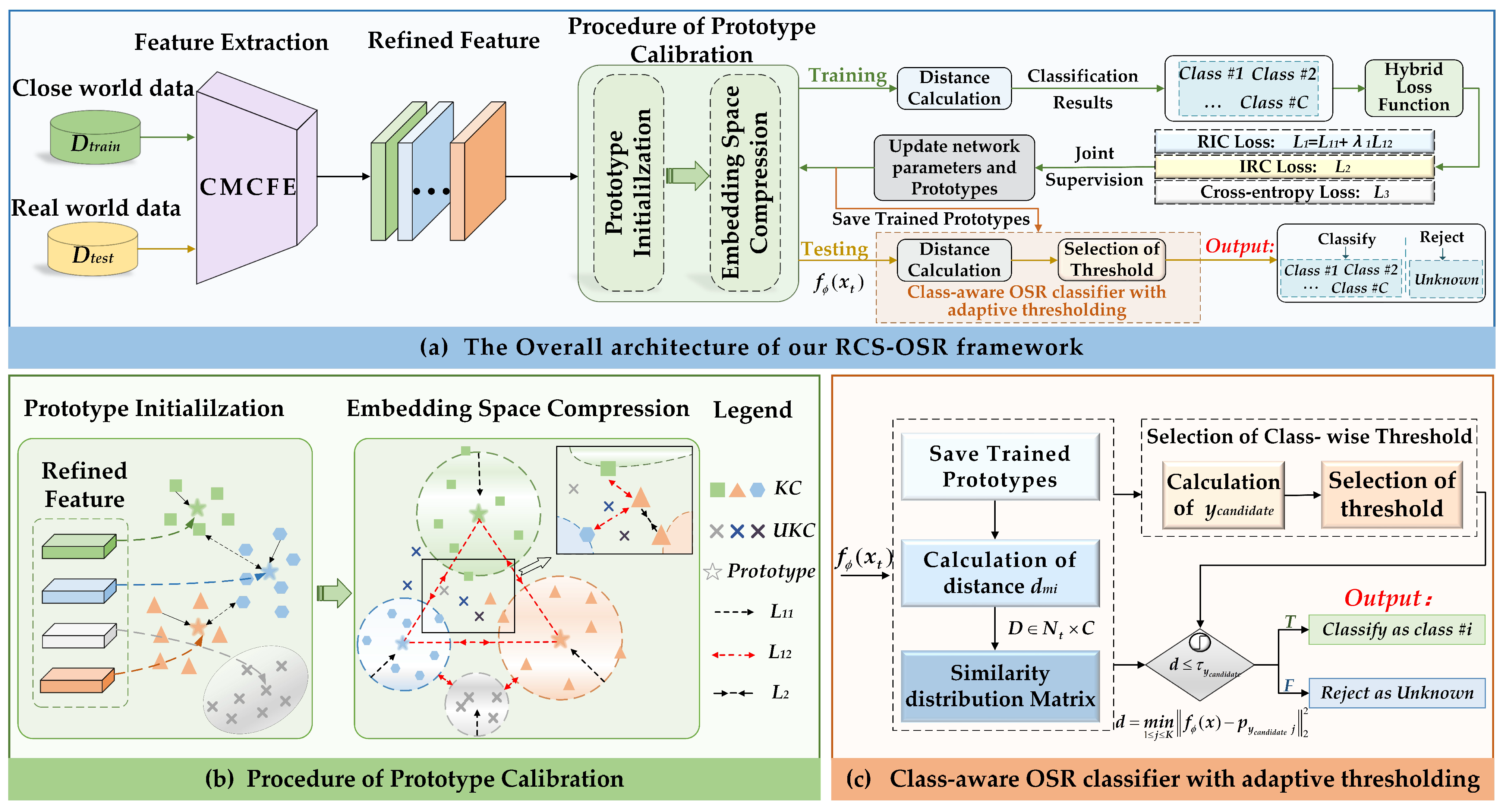
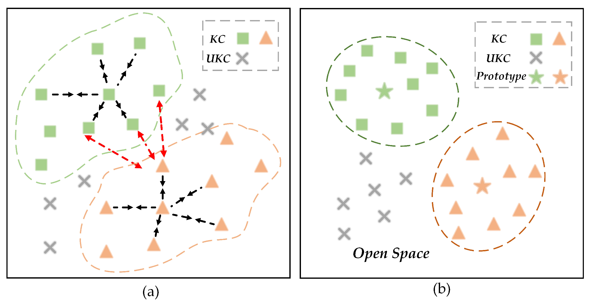
A novel RCS-OSR framework is proposed for classifying known classes and identifying unknown classes in open scenarios. By emphasizing reinforced class separability, this framework can effectively distinguish between known and unknown classes that are prone to confusion in open scenarios. By designing regularized intra-class compactness loss (RIC-Loss) and intra-class relationship aware consistency loss (IRC-Loss), along with joint supervised training that utilizes cross-entropy loss, it enhances the discriminability of the extracted features, balancing open space risk and empirical classification risk.

(2)

A CMCFE module with causal region-aware capability is proposed, which can enhance feature discriminability by strengthening the representation of causal regions through attention mechanisms. Furthermore, a multi-scale abstract features aggregation branch and an auxiliary handcrafted feature injection branch are employed to enhance the model’s capability in extracting information from local regions of diverse scales.

(3)

A class-aware OSR classifier with adaptive thresholding is proposed, which effectively leverages the differences between different classes. By calculating the distances between correctly classified samples and their corresponding prototypes during training, the similarity distribution matrix can be generated, with the queried maximum value serving as the adaptive threshold for this class of targets.

2. Related Works

2.1. Open Set Recognition

According to Geng et al., the OSR methods can be categorized into traditional machine learning-based (ML-based) and deep learning-based methods (DL-based) [12].

ML-based Models: While traditional ML-based methods have thrived in closed-set scenarios, their performance significantly diminishes in open scenarios. To accommodate the dynamic nature of open scenarios, Scheirer et al. [21] formulated mathematical definitions for open space risk and introduced the one-versus-set machine (1-VS-SET) to tackle the OSR problem. For better probabilistic modeling, Scheirer et al. [22] proposed the compact abating probability (CAP) theory, which suggests that the probability of a sample belonging to known classes decreases as it ventures into the open space. Drawing from CAP, Scheirer et al. [22] successively proposed the Weibull-calibrated support vector machine (W-SVM) model, leveraging insights from extreme value theory (EVT) and employing the Weibull distribution to model known classes. Additionally, Scherreik et al. introduced the probabilistic open set SVM (POS-SVM) [23] and the probabilistic open set SVM model via cross-validation (POS-SVM-CV) [24] for OSR. Rudd et al. [25] incorporated EVT into the classifier to achieve a more compact statistical model. Zhang et al. [26] introduced the sparse representation-based OSR model, which combines EVT with generalized sparse representation to model the tail distribution of reconstruction errors. Given that traditional ML-based algorithms require manual feature engineering, which is highly dependent on domain knowledge and expertise and is susceptible to noise and outliers, this paper focuses on DL-based models.

DL-based Models: Deep neural networks (DNNs) have been extensively utilized in computer vision tasks, yielding advanced results. However, these deep models often utilize SoftMax to normalize the classification logits, which results in an inherent closed-set property. Following [12], there are two lines of research in DL-based OSR models: discriminative-based and generative-based models.

The discriminative-based models focus on constraining the decision boundaries of known classes and identifying unknown classes through a threshold [12]. Bendale et al. [27] pioneered the adaptation of DNNs for OSR by substituting the SoftMax layer with the OpenMax layer. They calibrated the activation vector of a test sample using the Weibull distribution of known classes, thereby effectively transforming the OSR problem into a CSR problem with $K+1$ classes. Yoshihashi et al. [28] proposed a classification reconstruction learning approach for open set recognition, termed CROSR, which integrates supervised classification with unsupervised reconstruction. CROSR leverages latent representations to complement crucial features absent in the classification branch. Similarly, Poojan et al. [29] introduced a class conditioned autoencoder (C2AE) for open set recognition, employing both cross-entropy and conditional autoencoder loss functions. Sun et al. [30] proposed conditional Gaussian distribution learning (CGDL), which can learn distinct Gaussian distributions from diverse feature representations. Dang et al. [31] and Ma et al. [4] proposed SAR target OSR models with incremental learning ability, which refined decision boundaries and constructed probabilistic models using both positive and negative samples. Wang et al. [32] devised an entropy-aware meta-learning method for SAR target OSR, yielding a highly separable feature space. To explicitly optimize the embedding space, various approaches with distance-based loss were proposed to enhance the discriminability of feature representations. Miller et al. [33] introduced a novel loss term for OSR, named class anchor clustering loss, which encouraged known classes to cluster tightly around class-specific centers within the logit space.

The generative-based models aim to synthesize unknown classes using generative adversarial networks (GANs) and variational autoencoders (VAEs) [12]. Ge et al. [34] extended OpenMax by incorporating GANs to generate unknown classes for learning discriminative decision boundaries. Neal et al. [35] proposed a counterfactual image generation method (OSRCI) for the OSR problem. By training an encoder-decoder structure with adversarial loss, OSRCI can acquire an embedding space with manageable open space risk. Geng et al. [36] devised two approaches for generating SAR targets of unknown classes: spatial clipping generation (SCG) and weighted generation (WG). However, optimizing the embedding space solely through generative means may be constrained by the data distribution, limiting the variability of generated samples and diminishing the model’s classification performance. Recently, some hybrid models have emerged, yet they are heuristic and lack rigorous theoretical foundations [37].

2.2. Prototype Learning

The prototype serves as an average or optimal exemplar of a class, thereby offering a succinct representation for the entire class [17,18]. The most well-known prototype learning method is k-nearest neighbors (KNN) [38]. Based on KNN, Kohonen introduced learning vector quantization (LVQ) [39] to enhance computational efficiency. However, most of these previous works relied on manual feature engineering. Recently, there has been a trend towards integrating prototype learning with deep neural networks. Notable examples include GCPL, CPN, and RPL, as introduced in Section 1.

Prototype learning offers a powerful representation approach for classification [17]. Generally, it primarily focuses on minimizing the intra-class distance for known features, which aids in establishing a closed decision boundary but often ignores the potential risk of open space posed by unknown data. To bolster the model’s robustness against unknown data, we focus on enhancing the representation capability and optimizing the embedding space. Correspondingly, the CMCFE module is designed to integrate information from different modalities. Additionally, our hybrid loss function takes into account both the distance relationship between samples in local regions and the global spatial relationship during the prototype optimization process.

3. Methodology

To better address OSR problems, we first formalize its definition. Assuming a training set $D_{train}=\left\{(x_i,y_i)\right\}\subseteq X_{tr}\times K$ with K known classes, $y_i\in K=\{k_1,k_{2,}\cdots ,k_n\}$ is the label of $x_i$. The testing set $D_{test}=\left\{\left(\begin{array}{c}{x}_i,y_i\end{array}\right)\right\}\subseteq X_{te}\times \mathsf{\Omega }$ includes both K known classes and the potential unknown classes U, whose labels belong to $N+1$. The goal of OSR is to derive a model $f_{osr}$ based on $D_{train}$, which can accurately classify known data $\{x_i\in X_{te},y_i\in K\}$, and effectively identify unknown data $\{x_i\in X_{te},y_i\in U\}$ [40].

3.1. Overview of RCS-OSR

The overall architecture of our proposed RCS-OSR is illustrated in Figure 3a. In the training process, known classes from $D_{train}$ are first fed into the CMCFE module, from which refined features with enhanced discriminability can be extracted. The CMCFE module consists of a multi-scale abstract features aggregation branch and an auxiliary features injection branch, which will be introduced in detail in Section 3.2. Upon initializing the prototypes, we formulate a hybrid loss function to jointly supervise model training and calibrate the prototypes by optimizing the embedding space. This hybrid loss function comprises three components: RIC loss, IRC loss, and cross-entropy loss, with the RIC loss being a combination of $L_{11}$ and $L_{12}$. Figure 3b elucidates the principles of RIC loss and IRC loss in the prototype calibration procedure. By attracting samples to their corresponding prototypes and penalizing the distances between prototypes of different classes, the RCS-OSR method achieves reinforced class separability, thereby enhancing classification performance. Upon completion of the training, the prototypes associated with each category are saved.

In the testing phase, $D_{test}$ are utilized as input, which includes known and unknown classes. After calculating the distances between the test sample $f_{\varphi }\left(t\right)$ and the saved prototypes, a class-aware OSR classifier is introduced to assign adaptive thresholds for each class, as shown in Figure 3c. If the distance between the test sample and the nearest prototype is below the threshold, it is classified as a known class; otherwise, it is rejected as unknown. Next, we will provide a detailed description of the proposed methods and the implementation process in the following subsections.

3.2. Cross-Modal Causal Features Enhancement Module

For SAR-ATR, the discriminative information in the target and shadow regions is the basis for classification. Hence, these areas are termed causal regions, with their features referred to as causal features. Conversely, the background region is termed the non-causal region, with its features denoted as non-causal features [3,41]. Existing SAR-ATR experiments assume that datasets are sufficiently large, diverse in classes, and contain samples of each class in various background clutters [42]. However, the reality is that most publicly available datasets are confined to a single imaging environment and are of a small scale. In such cases, situations may arise where the background clutter region contains pseudo-discriminative information useful for inference, despite lacking information pertaining to the target’s geometric structures and electromagnetic scattering patterns. In this paper, we refer to the model’s acquisition of non-causal features as overfitting, which can have stochastic effects, either positive or negative.

Given the dynamic and open nature of real battlefield environments, it is imperative for the model to prioritize information directly pertaining to the target’s response while minimizing the influence of background clutters. Therefore, we introduce the CMCFE module to enable the extraction of robust and discriminative causal features. Moreover, the hybrid attention mechanism facilitates the dynamic adjustment of attention across image regions, allowing for adaptation to emerging novel features.

Figure 4 illustrates the detailed structure of the CMCFE module, comprising a multi-scale abstract features aggregation branch (as depicted in Figure 4a) and an auxiliary features injection branch (as depicted in Figure 4b). The CMCFE module mines rich information from SAR images by incorporating attention mechanisms to direct the model’s focus towards causal regions and by injecting handcrafted features as prior knowledge to enhance the feature representation ability. Figure 4c shows the process of fusing abstract features $F_A$ and handcrafted features $F_H$. Figure 4d provides the detailed implementation of three MSFE blocks shown in Figure 4a. Further elaboration on the CMCFE module will be provided subsequently.

3.2.1. Multi-Scale Abstract Features Aggregation Branch

For SAR OSR tasks, the models need to classify known classes and identify unknown ones, demanding more sophisticated feature extraction strategies. To fully exploit the rich information in SAR images, we introduce a multi-scale feature extraction block (MSFE) to extract both high-level semantic features and shallow structural features, thereby enhancing the model’s feature representation capability. Specifically, as shown in Figure 4a, the multi-scale abstract features aggregation branch contains three MSFE paths with different kernel sizes to extract features at different scales. The internal structure of the MSFE block is depicted in Figure 4d.

The MSFE block, following the convolution module, is composed of convolution, max pooling, dropout, and flattening layers, along with the parallel convolutional block attention (PCBAM) module to filter out the background information. As depicted in Figure 5, the PCBAM is used to compute channel attention and spatial attention [43], enabling the model to focus on causal areas. Following the mechanism of human visual information processing, the MSFE model begins with a sequence of three convolutional layers, each featuring varying kernel sizes to capture features at different scales. The detailed process unfolds as follows.

Given the input feature map $F_{in}\in {\mathbb{R}}^{C\times H\times W}$, where C, H, and W represent the number of channels, height, and width, respectively, three parallel branches employ convolutional kernels of different sizes to process $F_{in}$, yielding $F_{out1}\in {\mathbb{R}}^{C\times H\times W}$, $F_{out2}\in {\mathbb{R}}^{C\times H\times W}$, and $F_{out3}\in {\mathbb{R}}^{C\times H\times W}$, respectively. The kernel sizes for the three paths are set to $3\times 3$, $5\times 5$, and $7\times 7$, respectively. Subsequently, the features extracted from the three branches are aggregated to obtain the multi-scale feature $F_{outa}\in {\mathbb{R}}^{C\times H\times W}$. For each branch, MSFE applies convolution, max pooling, and dropout operations sequentially to process $F_{in}$ and obtain $F_{in}^{\prime }\in {\mathbb{R}}^{C\times H\times W}$, as depicted in Figure 4d. Next, $F_{in}^{\prime }$ serves as the input for PCBAM to compute channel and spatial attention maps, and obtain $F_{out}^{\prime }\in {\mathbb{R}}^{C\times H\times W}$. After the global average pooling (GAP) operation, the CNN abstract features $F_A\in {\mathbb{R}}^{C\times H\times W}$ are obtained, as shown in Figure 4a.

As illustrated in Figure 4d, the PCBAM block is embedded into the backbone network to optimize channel and spatial information. The detailed operation process of the PCBAM block, as depicted in Figure 5, comprises a channel attention module (CAM) and a spatial attention module (SAM) [43]. Specifically, CAM combines spatial information using both average pooling and max pooling operations. The extracted features are then passed through a shared network to generate the channel attention map $W_C\left(F_l\right)\in {\mathbb{R}}^{C\times 1\times 1}$.

$$W_C\left(F_l\right)=\sigma \left(MLP(A\nu gPool\left(F_l\right)+MaxPool\left(F_l\right))\right)$$

(1)

where $F_l\in {\mathbb{R}}^{C\times H\times W}$ denotes the input feature map. $\sigma$ is the sigmoid function, and $MLP$ denotes a shared multi-layer perceptron with one hidden layer. $AvgPool$ and $MaxPool$ represent average pooling and max pooling operations on the feature map, respectively.

SAM pays more attention to the target’s location information in the image, allowing the model to focus on crucial areas. SAM combines max pooling and average pooling to extract spatial features, then uses a $7\times 7$ convolutional layer to fuse the feature maps, generating the final spatial attention map $W_S\left(F_l\right)\in {\mathbb{R}}^{1\times H\times W}$ after activation.

$$W_S\left(F_l\right)=\sigma \left(f^{7\times 7}[A\nu gPool\left(F_l\right);MaxPool\left(F_l\right)]\right)$$

(2)

where $f^{7\times 7}$ denotes the convolutional operation with a $7\times 7$ kernel size. After acquiring both CAM and SAM branches, the output feature map $F_p\in {\mathbb{R}}^{C\times H\times W}$ is obtained through a parallel connection.

$$F_p=F_l\otimes W_S\left(F_l\right)+F_l\otimes W_C\left(F_l\right)$$

(3)

where ⊗ denotes the multiplication operation.

The parallel structure of PCBAM can flexibly integrate channel information and spatial information without the influence of sequential transmission, allowing each module to focus on different types of information. The integration of the attention mechanism enables the model to prioritize discriminative causal features crucial for the SAR OSR tasks [44]. Moreover, when encountering unknown classes, the model can focus on target areas, thereby minimizing the interference of irrelevant information and bolstering robustness in complex scenes.

3.2.2. Auxiliary Features Injection Branch

CNN eliminates the need for manual feature engineering but suffers from poor interpretability, which can be mitigated by injecting traditional handcrafted features [45]. Traditional handcrafted feature extraction methods for SAR images leverage expertise in target properties and electromagnetic scattering characteristics to enhance the discriminability and interpretability of features. Generally, handcrafted features can be divided into global and local features. Global features describe the overall distribution but may neglect local structures and details. Examples of such features include local binary pattern (LBP) [46] and histogram of oriented gradients (HOG) [47], etc. In contrast, local features capture key points for detailed texture and structure information, yet they are prone to interference from outliers, as seen in methods like scale invariant feature transform (SIFT) and speed up robust features (SURF), etc. [48]. To leverage the robustness of global features and the sensitivity of local features effectively, our method integrates both to achieve better discriminability.

As shown in Figure 4b, following the extraction of $F_{HOG}$ as the global feature and $F_{SIFT}$ as the local feature, we concatenate them to form a longer feature vector $F_H$.

$$F_H=Concat(N\left(F_{HOG}\right),N\left(F_{SIFT}\right))$$

(4)

where $Concat(·)$ denotes the concatenation operation, and  $N(·)$ represents normalization.

3.2.3. Cross-Modal Hybrid Feature Fusion Block

Given the substantial disparities in dimensions and semantics between traditional handcrafted features $F_H\in {\mathbb{R}}^{C\times H\times W}$ and deep abstract features $F_A\in {\mathbb{R}}^{C\times H\times W}$, employing linear concatenation to fuse features from different modalities may compromise the quality of the output features, thereby limiting the model’s performance [45]. To leverage the differences and correlations between the two modal features and alleviate information dilution during feature fusion, this paper introduces a cross-modal hybrid feature fusion block ($CMH{F}^2$), as illustrated in Figure 4c. It aims to optimally exploit the inherent complementary relationship between handcrafted features and abstract features for their mutual enhancement.

In $CMH{F}^2$, we initially adopt a $1\times 1$ convolutional layer to compress the channels. Then, the cross-multiplication operation is utilized to enhance the correlation between the two cross-modal features and effectively suppress irrelevant ones. The detailed process is outlined as follows:

$$F_A^{\prime }=Con{\nu }_{1\times 1}\left(F_A\right)\otimes Con{\nu }_{1\times 1}\left(F_H\right),F_H^{\prime }=Con{\nu }_{1\times 1}\left(F_H\right)\otimes Con{\nu }_{1\times 1}\left(F_A\right)$$

(5)

where $Conv{\nu }_{1\times 1}(.)$ denotes the $1\times 1$ convolutional layer, and ⊗ represents the multiplication operation.

Next, we employ the PCBAM block to enhance the representation of cross-modal features in both the spatial and channel dimensions, thereby improving the response of causal features. Additionally, skip connections are adopted to mitigate the dilution of information.

$$F_A^{″}=PCBAM\left(F_A^{\prime }\right)\oplus F_A,F_H^{″}=PCBAM\left(F_H^{\prime }\right)\oplus F_H$$

(6)

where $PCBAM(·)$ and ⊕ represent PCBAM block and addition operation, respectively.

To fully mine the heterogeneity of cross-modal features, we concatenate the self-enhanced features and feed them into a $3\times 3$ convolutional layer for feature refinement.

$$F_{CM}=Con{\nu }_{3\times 3}\left(Concat(F_A^{″},F_H^{″})\right)$$

(7)

where $F_{CM}$ denotes the output feature, and $Conv{\nu }_{3\times 3}(.)$ denotes the $3\times 3$ convolutional layer, and $Concat(·)$ represents the concatenation operation.

Finally, we introduce skip connections to capture residual information, thereby better retaining and utilizing the differences between original features.

$$F_{out}=Con{\nu }_{3\times 3}\left(Concat(F_{CM},F_A,F_H)\right)$$

(8)

where $F_{out}\in {\mathbb{R}}^{C\times H\times W}$ represents the output feature refined by the $CMH{F}^2$ block. $F_{out}$ can also be expressed as $f_{\varphi }\left(x\right)$. Specifically, x denotes the input image, and  $f_{\varphi }(·)$ represents the function representation of the CMCFE module, where $\varphi$ is the set of parameters for the CMCFE module.

3.3. Hybrid Loss for Discriminative Prototype Learning

The positional relationship between different classes can be characterized by intra-class compactness and inter-class separation. In Figure 6a, the black double dashed arrows represent intra-class compactness, showing how closely instances of the same class are clustered. The closer the instances with the same label are, the more compact the clusters become, indicating higher intra-class compactness. Similarly, inter-class separation is depicted by red double dashed arrows, illustrating the distance between samples with different labels in the embedding space. The farther apart samples of different classes are, the stronger the model’s classification ability.

As mentioned above, constructing an embedding space with reinforced class separability is crucial for improving the performance of OSR. As shown in Equation (9), the center loss [49] can increase intra-class compactness by minimizing the distance between a sample and its corresponding prototype. As illustrated in Figure 6b, prototype learning promotes a more compact embedding space under the constraint of center loss.

$$L_{center}={\displaystyle \frac{1}{2}}\sum _{1\le l\le M}{∥f_{\varphi }\left(x_l\right)-p_{ij}∥}_2^2$$

(9)

where $f_{\varphi }\left(x_l\right)$ represents the feature vector of the test sample $x_l$ and $\left\{P_{ij}|j\in \{1,2,\cdots K\}\right\}$ denotes the prototypes corresponding to class $i\in \{1,2,\cdots C\}$, with  K denoting the number of prototypes in each class and C being the number of known classes.

It can be found that $L_{center}$ only focuses on making the samples of the same class closer in the embedding space, but it does not directly affect the distances between samples of different classes, since there are no prototypes involved in their loss calculation. Furthermore, we have observed that $L_{center}$ only considers the distance between a sample and its corresponding prototype. It treats samples with the same distance to the prototype equally, disregarding their distribution around the prototypes. This may result in samples with equal distances to the prototype being uniformly distributed in concentric circles, which induces cluster overlapping.

Motivated by this, we thoroughly explore a feature constraint method based on regularization techniques to boost both intra-class compactness and inter-class separation, as shown in Figure 3b. Our proposed RIC-Loss, as shown in Equation (10), extends the original center loss by incorporating two additional regularization constraint terms. Specifically, $L_{11}$ constrains the distance between samples and their corresponding prototypes, while $L_{12}$ penalizes the distances between prototypes of different classes.

$$L_1=L_{11}+{\lambda }_1{L}_{12}$$

(10)

$$L_{11}={\displaystyle \frac{1}{2}}\sum _{1\le l\le M}\delta ({∥f_{\varphi }\left(x_l\right)-p_{ij}∥}_2^2>{\gamma }_1)·{∥f_{\varphi }\left(x_l\right)-p_{ij}∥}_2^2$$

(11)

$$L_{12}={\displaystyle \frac{1}{{\sum }_{1\le i,k<C,i\ne k}\delta \left({∥p_{ij}-p_{kj}∥}_2^2>{\gamma }_2\right)·{∥p_{ij}-p_{kj}∥}_2^2+\epsilon }}$$

(12)

In Equation (10), ${\lambda }_1$ is a hyperparameter used to balance the effects of $L_{11}$ and $L_{12}$. In our experiments, ${\lambda }_1$ is set to 1. Specifically, the first term in Equation (10) is shown in Equation (11), where $\delta \left(condition\right)=1$ if the $condition$ is satisfied, and $\delta \left(condition\right)=0$ if not. ${\gamma }_1$ is a regularization term employed to constrain the intra-class distance.

The second term of Equation (10) is shown in Equation (12). $L_{12}$ serves as a penalty term for the distance between prototypes of different classes. During training, prototypes of different classes tend to move away from each other, as shown in Figure 3b. In Equation (12), $p_{ij}$ and $p_{kj}$ represent the prototypes corresponding to class i and k, respectively, with $i\ne k$. Additionally, ${\gamma }_2$ is a regularization term designed to constrain the distances between different prototypes, where $\epsilon$ is a constant term greater than 0. When the distance between prototypes of different classes falls below ${\gamma }_2$, $\epsilon$ can slow down the update speed of the model parameters, thereby enhancing the model’s robustness. To simplify hyperparameter configurations, we set ${\gamma }_1$ and ${\gamma }_2$ as learnable parameters and update them in a data-driven manner.

To further optimize the embedding space, the IRC-Loss, as illustrated in Equation (13), is proposed to constrain the label consistency among nearest-neighbor samples, thereby promoting intra-class compactness. In Equation (13), $d(f_{\varphi }\left(x_i\right),f_{\varphi }\left(x_j\right))$ denotes the distance between two feature vectors, $m_c$ represents the sample set belonging to class ‘c’ in the current mini-batch, and T is the temperature factor. Specifically, T is set to the variance of all sample feature vectors within the current mini-batch, denoted as $T={\sigma }^2$.

$$L_2=-{\displaystyle \frac{1}{M}}\sum _{i\in 1\dots M}log\left({\displaystyle \frac{{\sum }_{i,j\in 1\dots m_c,j\ne i}{e}^{-d(f_{\varphi }\left(x_i\right),f_{\varphi }\left(x_j\right))/T}}{{\sum }_{k\in 1\dots M,k\ne i}{e}^{-d(f_{\varphi }\left(x_i\right),f_{\varphi }\left(x_k\right))/T}}}\right)$$

(13)

The previously designed loss functions $L_1$ and $L_2$ optimize the prototype distribution by incorporating regularization terms. However, they neglect the separability of different classes. Inspired by Wen et al. [49], we incorporated the cross-entropy loss function $L_3$ to emphasize the overall distribution and the model’s classification performance. $L_3$ is placed behind the classification layer and computes the penalty term by assessing the difference between the predicted label and the ground-truth label, thereby enhancing the model’s classification capabilities. $L_3$ is expressed as:

$$L_3=-{\displaystyle \frac{1}{M}}\sum _{1\le l\le M}logp(y_l=k|x_l)$$

(14)

For obtaining prototype representations with reinforced class separability, three distinct loss functions are integrated collaboratively to supervise the training.

$$L_h={\omega }_1{L}_1+{\omega }_2{L}_2+L_3$$

(15)

where ${\omega }_1$ and ${\omega }_2$ are hyperparameters used to balance the contribution of the first and second terms. Specifically, we set ${\omega }_1=0.7$ and ${\omega }_2=0.5$.

Algorithm 1 delineates the comprehensive procedures for implementing the proposed RCS-OSR. During training, only $D_{train}$ with known classes is utilized and the hybrid loss is employed for supervision.

Algorithm 1 Pseudo-code of the Proposed RCS-OSR Algorithm

Input: Known class targets $D_{train}$ for training, hyperparameters: ${\gamma }_1$, ${\gamma }_2$, ${\lambda }_1$, ${\omega }_1$, ${\omega }_2$, initialized learning rate $l=0.001$, and the number of training iterations $t=0$. Output: The set of parameters for the CMCFE module $\varphi$, and all saved prototypes $p_{ij}$.   1: Initialize CMCFE module and all prototypes.   2: while training not converge do   3:    $t=t+1$   4:    Select a mini-batch M samples from $D_{train}$ and feed them into our model   5:    Calculate the representation loss $L_1$, $L_2$ and classification loss $L_3$, respectively.   6:    Calculate the hybrid loss $L_h={\omega }_1{L}_1+{\omega }_2{L}_2+L_3$   7:    Compute the backpropagation gradients $\partial L_h/\partial \varphi$ and $\partial L_h/\partial p_{ij}$   8:    Update the CMCFE module parameters ${\varphi }^{t+1}$ by ${\varphi }^{t+1}={\varphi }^t-l^t·(\partial L_h^t/\partial {\varphi }^t)$   9:    Calibrate the prototypes $p_{ij}^{t+1}$ by $p_{ij}^{t+1}=p_{ij}^t-l^t·(\partial L_h^t/\partial p_{ij}^t)$ 10: end while

3.4. Class-Aware OSR Classifier with Adaptive Thresholding

Facing unknown inputs from novel classes, an intuitive approach for classification is to impose a threshold over the output distance [18]. It assumes that unknown classes typically reside far from the prototypes of known classes. However, DL-based methods are prone to overfitting the training data, resulting in excessively confident predictions. Therefore, they assign high probabilities even to unknown classes, making the threshold difficult to tune. Additionally, due to the unique semantic information of known classes in different tasks, it is challenging to determine a universal threshold suitable for all OSR tasks.

To exploit the differences among classes, we dynamically assign a class-aware threshold for each class according to the distance distribution, as shown in Figure 3c. Particularly, after training, we can obtain the feature vector $f_{\varphi }\left(x_m\right)$ of the correctly predicted sample $x_m$, and the prototypes $p_{ij}$ of each class. Then, we can generate the similarity distribution matrix $D\in N_t\times C$ for each class by calculating the Euclidean distance between them.

$$D=\left\{d_{mi}={∥f_{\varphi }\left(x_m\right)-p_{ij}∥}_2^2\right\}$$

(16)

where $i\in \{1,2,\cdots C\}$, $m=1,2,\dots ,N_{{ }_t}$, $N_t$ denotes the number of samples per class. The element $d_{mi}$ in row m, column i of the similarity distribution matrix signifies the Euclidean distance between sample $x_m$ and its corresponding prototype $p_{ij}$.

For each test sample $x_t$, the label corresponding to the nearest prototype is selected as its candidate label, denoted as $y_{candidate}$. Subsequently, the distance distribution of the class $y_{candidate}$ in the similarity distribution matrix D can be obtained by using $y_{candidate}$ as the column index value. The maximum distance element value $d_{y_{candidate}}={max}_{1\le m\le N_t}{d}_{m{y}_{candidate}}$ is then designated as the adaptive threshold ${\tau }_{y_{candidate}}$ for the class $y_{candidate}$. Finally, the classification rules are presented in Equation (17), if the distance between a test sample $x_t$ and its nearest prototype is less than the corresponding threshold ${\tau }_{y_{candidate}}$ of that prototype, it is classified into that class; otherwise, it is identified as the unknown class.

$$y_{pred}=\left\{\begin{array}{cc}{y}_{candidate},\hfill & \underset{1\le j\le K}{min}{∥f_{\varphi }\left(x_t\right)-p_{y_{candidate}j}∥}_2^2\le {\tau }_{y_{candidate}}\hfill \\ \\ unknown,\hfill & \underset{1\le j\le K}{min}{∥f_{\varphi }\left(x_t\right)-p_{y_{candidate}j}∥}_2^2>{\tau }_{y_{candidate}}\hfill \end{array}\right.$$

(17)

4. Experiments and Results

4.1. Experimental Setup

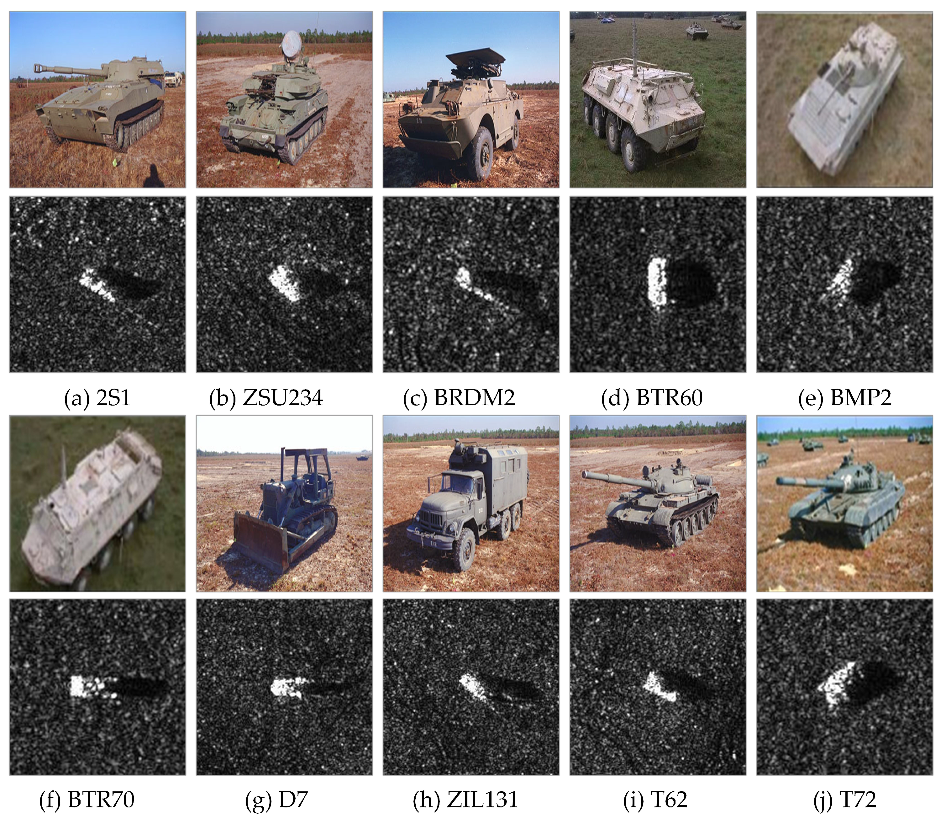
4.1.1. Dataset Description and Implementation Details

The MSTAR dataset, provided by Sandia National Laboratory in the U.S., operates in the X-band frequency and HH polarization mode, with a resolution of 0.3 m × 0.3 m. Figure 7 shows the SAR images and their corresponding optical images. It includes ten vehicle classes with different depression and azimuth angles, as detailed in

Table 1. Detailed information of the MSTAR dataset under SOC.

Type	Train	Number	Test	Number
1-2S1	17${ }^{\circ }$	299	15${ }^{\circ }$	274
2-ZSU234	17${ }^{\circ }$	299	15${ }^{\circ }$	274
3-BRDM2	17${ }^{\circ }$	298	15${ }^{\circ }$	274
4-BTR60	17${ }^{\circ }$	256	15${ }^{\circ }$	195
5-BMP2	17${ }^{\circ }$	233	15${ }^{\circ }$	195
6-BTR70	17${ }^{\circ }$	233	15${ }^{\circ }$	196
7-D7	17${ }^{\circ }$	299	15${ }^{\circ }$	274
8-ZIL131	17${ }^{\circ }$	299	15${ }^{\circ }$	274
9-T62	17${ }^{\circ }$	299	15${ }^{\circ }$	273
10-T72	17${ }^{\circ }$	232	15${ }^{\circ }$	196
Total		2747		2425

. The training and testing sets are based on depression angles of ${17}^{\circ }$ and ${15}^{\circ }$, respectively.

In this paper, the model was trained using the Adam optimizer for 120 epochs with a batch size of 128. We implemented a learning rate decay strategy, starting from 0.001. Throughout all experiments, each class was assigned a corresponding prototype. Additionally, the SAR images were uniformly cropped to a size of $64\times 64$.

4.1.2. Evaluation Protocols

We randomly select several classes from the MSTAR dataset as known classes for training and assign the remainder as unknown ones. During testing, we employ all ten target classes. Following [12], we use Openness to denote the ratio of known classes to unknown classes, which represents the complexity of the OSR task.

$$Openness=1-\sqrt{{\displaystyle \frac{2·N_{train}}{N_{target}+N_{test}}}}$$

(18)

where $N_{train}$ and $N_{target}$ represent the number of known classes during training and testing, respectively, $N_{test}$ represents the total number of classes during testing, and $N_{train}=N_{target}$.

For comprehensive evaluation, we select several metrics, including $precision$, $recall$, $F{1}_{macro}$ and $accuracy$. Specifically, $accuracy$ reflects the model’s overall accuracy across all samples. $F{1}_{macro}$ calculates the mean $F1$ scores across all classes, where $F1$ is the harmonic mean of $precision$ and $recall$. The definitions of these metrics are as follows:

$$accuracy={\displaystyle \frac{{\sum }_{i=1}^{M}T{P}_{ii}}{N_{total}}}$$

(19)

$$precision={\displaystyle \frac{{\sum }_{i=1}^M{p}_i}{M}},p_i={\displaystyle \frac{T{P}_i}{T{P}_i+F{P}_i}}$$

(20)

$$recall={\displaystyle \frac{{\sum }_{i=1}^M{r}_i}{M}},r_i={\displaystyle \frac{T{P}_i}{T{P}_i+F{N}_i}}$$

(21)

$$F{1}_{macro}={\displaystyle \frac{{\sum }_{i=1}^{M}F{1}_i}{M}},F{1}_i=2\times {\displaystyle \frac{precisio{n}_i\times recal{l}_i}{precisio{n}_i+recal{l}_i}}$$

(22)

where M denotes the number of target classes and $N_{total}$ represents the total test instances.

4.2. Comparison with Other OSR Methods

To verify the effectiveness of our proposed method, several DL-based OSR algorithms are selected for comparison. The detailed introductions are as follows:

(1)

SoftMax compares the highest probability with a threshold for open set recognition.

(2)

OpenMax substitutes the SoftMax layer with the OpenMax layer to generate probabilities for unknown classes and converts the OSR task into a CSR task with $K+1$ classes [27].

(3)

GCPL calculates the distances among prototypes for classification. Additionally, GCPL combines discriminative and generative losses to reduce open space risk [17].

(4)

CGDL proposes a novel method, conditional Gaussian distribution learning, based on the variational auto-encoder, which can classify known classes by forcing different latent features to approximate different Gaussian models [30].

(5)

CAC allocates anchored class centers to known classes to increase intra-class compactness, which can reserve extra space for the emergence of unknown classes [33].

(6)

ARPL introduces an adversarial margin constraint to confine the open space based on RPL. Additionally, it devised an instantiated adversarial enhancement method to generate diverse unknown classes [20].

4.2.1. Performance Comparison on the MSTAR Dataset

For a fair comparison, we adopt the experimental setups from Ma et al. [50] and Geng et al. [36]. Specifically, BMP2, BTR70, and T72 are chosen to constitute the training set, while the test set encompasses all 10 classes. During the evaluation phase, $precision$, $recall$, $F{1}_{macro}$, and $accuracy$ are employed.

Table 2. OSR performance of different methods on the MSTAR dataset (Bold and underline indicate the highest and second maximum values in the respective column).

Methods	OSR Performance (%)
	Recall	Precision	$\mathit{F}{\mathbf{1}}_{\mathit{macro}}$	Accuracy
SoftMax	65.7	65.4	64.2	-
OpenMax	76.0	67.8	67.5	78.2
OSmIL	93.4	87.0	89.9	93.7
CGDL	90.7	85.1	87.6	92.5
CAC	84.8	88.4	86.2	92.4
EVM	90.5	81.0	85.0	91.8
GCPL	86.3	73.1	78.3	85.6
ARPL	68.8	55.6	59.4	71.9
GvRSC	73.2	67.8	69.2	-
Ours	94.1	87.8	90.7	94.2

shows the performance comparison of different methods. Our proposed algorithm outperforms the others in three OSR metrics. The $recall$ and $precision$ of other methods have exhibited varying degrees of decline, which may be attributed to overfitting the training data, leading to decreased performance. In particular, SoftMax captures only rudimentary discriminative features of known classes but struggles to provide a comprehensive representation, resulting in poor performance in identifying unknown classes with an $F{1}_{macro}$ of 64.2%. While OpenMax slightly boosts OSR performance, the inherent similarity between known and unknown classes curtails its efficacy. Compared with SoftMax, it only increases by 3.3%.

Autoencoder (AE)-based methods, such as CGDL, are adept at acquiring diverse low-dimensional feature representations through data reconstruction. However, they exhibit two notable limitations: the pixel-level reconstruction often retains background information extraneous to the targets, thereby impeding the model’s ability to capture discriminative features. Additionally, such irrelevant information can interfere with the classification of known classes, leading to a reduction in the accuracy of CSR. In contrast to AE-based methods, RCS-OSR can maintain high accuracy for the CSR task while also improving several OSR metrics by 3.4%, 2.7%, 3.1% and 1.7%, respectively. This is because it can enhance the discriminability of target features by guiding the model to focus on causal areas and employing a hybrid loss for supervised learning. Similarly, when compared with other discriminative models, such as CAC and OSmIL, RCS-OSR also demonstrates its superiority by optimizing the embedding space and incorporating a class-aware classifier to reinforce class separability.

Compared to generative models like ARPL and GvRSC, RCS-OSR shows superior improvements of 25.3%, 32.2%, 31.3% and 22.3%, respectively. This is because generative models may struggle with data generation due to constraints of the training data and may not generalize well to unseen classes. In contrast, RCS-OSR employs a more flexible discriminative model to effectively adapt to diverse distributions. In conclusion, RCS-OSR ensures both accurate classification of known classes and precise identification of unknown classes simultaneously, thereby effectively addressing the challenges in open scenarios.

Figure 8 illustrates the confusion matrix for various methods. It reveals that other methods experience significant confusion between certain classes in open scenarios. Specifically, despite ARPL’s superior performance on natural images, its efficacy on SAR datasets is suboptimal. Most unknown classes are erroneously classified as known ones, leading to significant confusion among different classes. Furthermore, the classification capability for known classes is significantly diminished. This shortfall can be attributed to the generative strategy employed by ARPL, which struggles to capture the discriminative features inherent in SAR images. The EVM enhances the model’s capacity for recognizing unknown classes by incorporating extreme value theory to align with the tail distribution. However, it fails to sustain the model’s high-precision performance in closed-set classification tasks. While discriminative models such as CAC, CGDL, and GCPL have improved the open set recognition performance of the model, they remain susceptible to missed and false alarms when encountering targets of unknown classes.

In contrast, our proposed algorithm exhibits accurate identification of unknown classes, while maintaining high classification accuracy for known classes, effectively alleviating confusion. Additionally, the true positive rate ($TPR$) and false positive rate ($FPR$) are derived from the confusion matrix, as shown in

Table 3. Comparisons of different methods for receiving known classes and identifying unknown ones (%) (Bold and underline indicate the highest and second maximum values in the respective column).

Methods	Classifying Known: TPR	Identifying Unknown: 1-FPR
OSmIL	93.4	93.1
EVM	91.8	92.3
OpenMax	74.9	79.3
CAC	81.09	96.34
CGDL	90.09	93.36
GCPL	86.69	85.36
ARPL	68.21	73.31
Ours	94.38	94.23

. The proposed algorithm can classify known classes with a $TPR$ of 94.38%, which is 0.98% higher than that of OSmIL. Although CAC has slightly better identification ability for unknown classes, it significantly compromises the classification accuracy for known classes. In conclusion, the proposed algorithm offers precise and dependable classification results.

Figure 9 provides an intuitive comparison of the OSR performance across various methods. It is obvious that the proposed RCS-OSR is situated at the upper left corner, indicating high $TPR$ and low $FPR$, which demonstrates its superiority. Specifically, the $TPR$ for our proposed algorithm is 94.38%, demonstrating a robust classification capability for known classes. Although its $FPR$ is marginally worse than that of the CAC, the $TPR$ significantly surpasses that of CAC. This disparity arises because CAC employs anchored class centers for diverse targets, requiring careful selection of the anchor magnitude to achieve optimal performance. Consequently, there is a propensity for known classes to be misidentified as unknown ones. Furthermore, the immobility of the class center hinders its ability to fully leverage the global spatial distribution information, potentially leading to open space risk.

In contrast, our proposed RCS-OSR sets the class center as a learnable parameter, assigns one or more prototypes to each class, associates them with their corresponding embedding features via a hybrid loss, and continuously optimizes these during training. Therefore, RCS-OSR can capture potential spatial distribution information more flexibly and comprehensively. In conclusion, our proposed RCS-OSR can precisely classify known classes and simultaneously identify unknown ones.

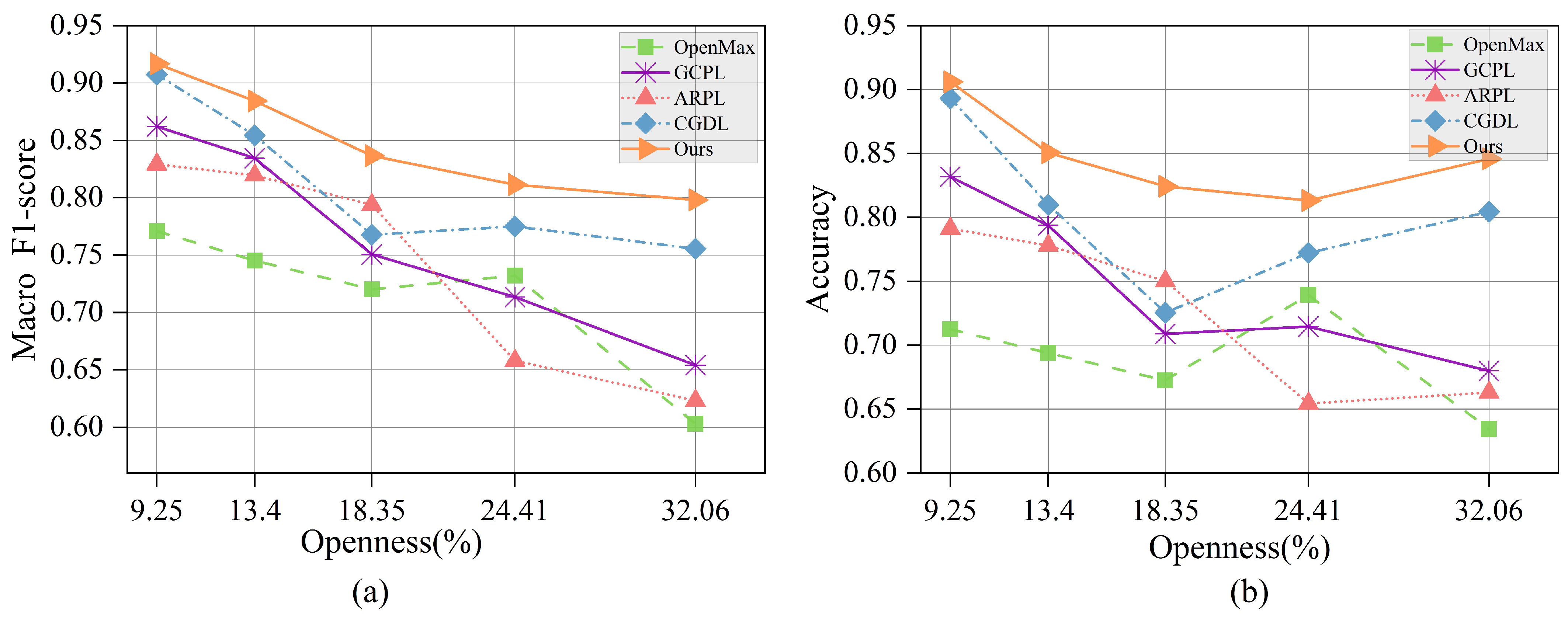
4.2.2. Performance Comparison Against Various Openness and Epochs

To assess the model’s performance under various levels of $Openness$, we randomly selected classes [7, 6, 5, 4, 3] as known data, while the remaining classes [3, 4, 5, 6, 7] were considered unknown data, resulting in an $Openness$ range from 9.25% to 32.06%.

As illustrated in Figure 10, the open space risk escalates with the increase in $Openness$, leading to serious confusion between different classes and a decline in OSR performance across all methods. There is a clear performance stratification among different methods. RCS-OSR notably outperforms OpenMax and GCPL, particularly in scenarios with high $Openness$. This proves that optimizing the prototype distribution can construct more distinct decision boundaries, thereby improving resilience against open space risk. Moreover, it is evident that the performance fluctuation of RCS-OSR across various levels of $Openness$ is merely 11.87%, surpassing the second-ranking method, CGDL, by 3.32%. This underscores its robustness and superior resilience against the open space risk across diverse scenarios.

Figure 11a presents the confusion matrix under an $Openness$ condition of 0, corresponding to a closed-set scenario. The results indicate that the proposed RCS-OSR exhibits minimal misclassifications and achieves high recognition accuracy. As $Openness$ increases, both the number of unknown classes and the risk associated with open space rise. Nevertheless, the algorithm maintains robust classification capabilities. Notably, in environments with low levels of $Openness$, the algorithm demonstrates strong recognition of unknown classes, suggesting that it can establish a more distinct decision boundary. In contrast, even when faced with high $Openness$ and some misclassifications of unknown classes as known ones, the algorithm retains high accuracy in both known class classification and unknown class recognition, demonstrating its robust classification performance.

5. Discussion

5.1. Ablation Studies

The proposed RCS-OSR reinforces class separability by optimizing both the prototype representation and its distribution. To verify the performance gains of each component, we conducted ablation studies on the MSTAR dataset with four randomly selected known classes and six unknown classes.

As shown in

Table 4. Progressive ablation experiments on the MSTAR dataset (%) (Bold and underline indicate the highest and second maximum values in the respective column).

MSFE	Auxiliary Features	CMHF2	Hybrid Loss	OSR Performance
				$\mathit{F}{\mathbf{1}}_{\mathit{macro}}$	Accuracy
-	-	-	-	74.26	73.03
✓	-	-	-	77.10	75.75
✓	✓	-	-	77.66	76.37
✓	✓	✓	-	78.63	77.44
✓	✓	✓	✓	81.50	81.60

, “Baseline” denotes the baseline model. Meanwhile, “MSFE”, “Auxiliary features branch”, “CMHF2”, and “Hybrid Loss” represent four strategies designed to enhance the network structures and optimize the embedding space. The $accuracy$ and $F{1}_{macro}$ of these four strategies outperform those of the baseline model. The first three strategies effectively enhance the model’s feature representation capability by aggregating multi-scale features and injecting handcrafted features, thus obtaining more discriminative prototype representations. Compared to others, the hybrid loss yields the most significant performance improvement, with $F{1}_{macro}$ increasing by 2.87% and $accuracy$ by 4.16%. This improvement is attributed to the model’s ability to simultaneously enhance intra-class compactness and inter-class separation under the supervision of hybrid loss, leading to a prototype distribution with reinforced class separability. When the aforementioned four strategies are combined, the performance is further improved.

5.2. Performance Comparison with Different Loss Functions

The distance-based loss functions attract positive samples while repelling negative samples, thus aiding in the learning of more discriminative features. Building on this, our proposed hybrid loss can further refine the prototype representation by incorporating regularization constraints. To validate its effectiveness, we have chosen center loss [49] for comparison.

As shown in

Table 5. OSR performance comparison of our hybrid loss and other distance-based losses (%) (Bold and underline indicate the highest and second maximum values in the respective column).

Loss Function	$\mathit{F}{1}_{\mathit{macro}}$	Accuracy
Cross Entropy	67.25	66.27
Center Loss	74.52	74.02
Center Loss + $L_1$	78.11	77.67
Center Loss + $L_1$ + $L_2$	79.24	79.51
Ours	81.50	81.60

, our hybrid loss achieves the best performance on all metrics. Specifically, center loss shows an improvement of 7.27% and 7.75% compared to the cross-entropy loss. This improvement is attributed to center loss’s capability to minimize intra-class differences by optimizing the distance between samples and their corresponding centers, thereby yielding more compact feature representations. Upon incorporating the $L_1$ constraint based on center loss, there is a respective increase of 3.59% and 3.65%. This indicates that $L_1$ can further optimize the prototype distribution. Upon adding the $L_2$ constraint, the performance is further improved, demonstrating that the $L_2$ effectively constrains label consistency, thereby obtaining feature representations with reinforced class separability. Furthermore, after integrating cross-entropy loss, the model can effectively utilize inter-class supervision information to enhance its classification capability.

5.3. Effectiveness Evaluation of CMCFE

The RCS-OSR enhances the model’s feature representation ability by incorporating handcrafted features and cross-modal feature fusion techniques. In this section, we conducted experiments to validate its effectiveness, as detailed in

Table 6. Effectiveness evaluation of the CMCFE module (%) (Bold and underline indicate the highest and second maximum values in the respective column).

Fusion Strategy	$\mathit{F}{1}_{\mathit{macro}}$	Accuracy
Baseline	78.33	77.39
Method 1	78.36	77.32
Method 2	79.52	78.36
Ours	80.93	81.14

.

“Baseline” represents the use of only CNN abstract features without any injection of handcrafted features. Conversely, “Method 1” and “Method 2” denote the application of direct concatenation and weighted concatenation strategies, respectively, to fuse the cross-modal features [45]. With the injection of handcrafted features, both “Method 1” and “Method 2” outperform the “Baseline”. This is because the handcrafted features leverage expertise and encompass information about the target’s structures, texture, and other characteristics. To some extent, these features can compensate for potential deficiencies or missing information in abstract features, and richer information can improve the model’s classification performance.

It is noteworthy that despite a slight improvement in the $F{1}_{macro}$ of “Method 1”, there is a decline in $accuracy$, suggesting that the direct concatenation strategy may induce learning ambiguity and yield adverse outcomes. Compared to “Method 1” and “Method 2”, the proposed RCS-OSR shows improvements of 2.6% and 3.75% over them, respectively. This is because the CMCFE module can guide the model to concentrate on causal areas, thereby extracting more discriminative features. Moreover, the designed cross-modal feature fusion strategy can effectively integrate information, leading to better performance gains.

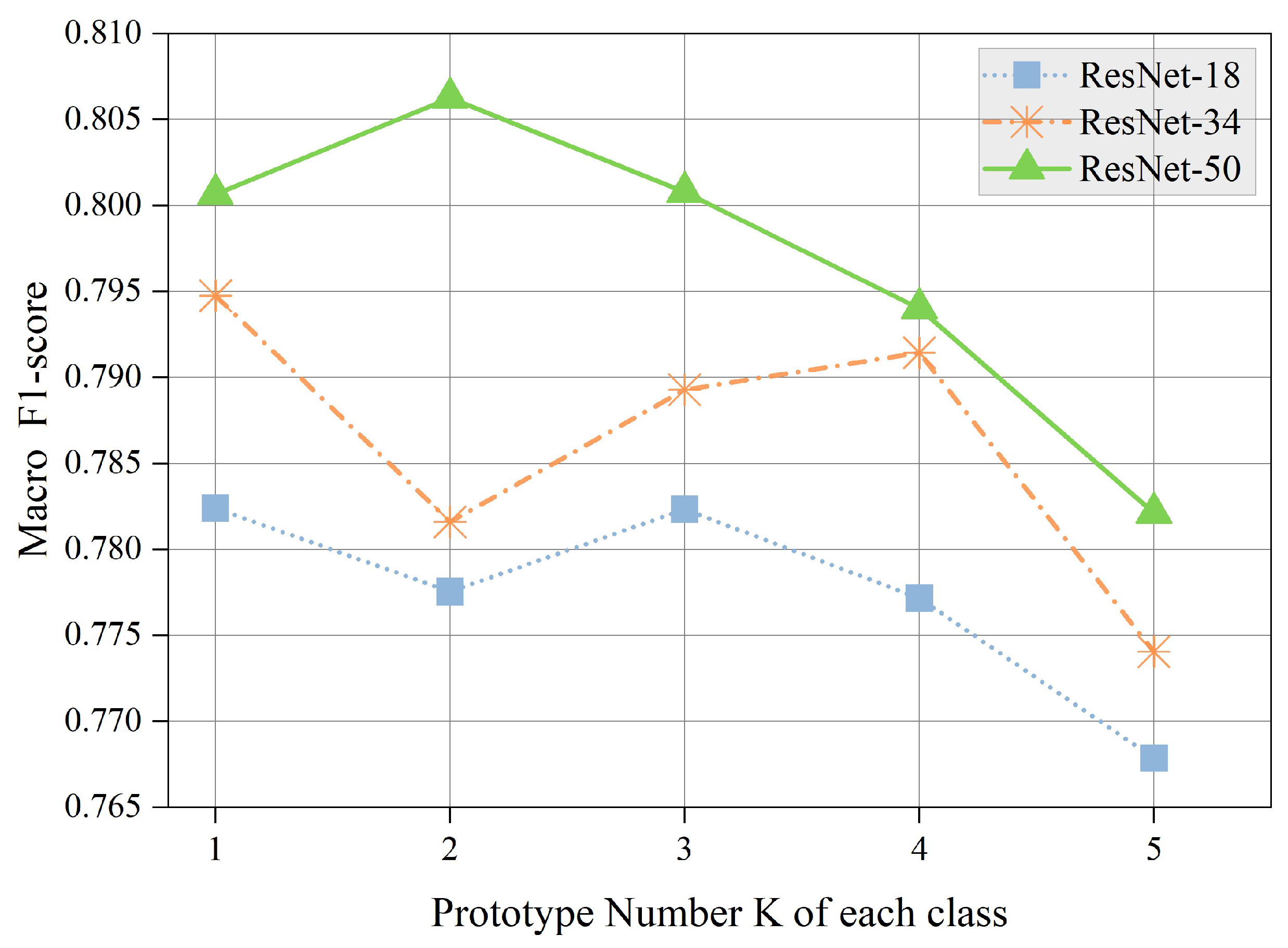
5.4. Influence of Prototype Number K

In prior experiments, each class was assigned only one prototype. To investigate the impact of varying the number of prototypes, we conducted trials across three distinct network architectures: ResNet-18, ResNet-34, and ResNet-50 [51]. As shown in Figure 12, setting more prototypes can better represent the internal differences between classes, thereby facilitating recognition performance. Nevertheless, it is observed that a surge in the number of prototypes does not significantly boost performance and may even lead to a decline.

This phenomenon can be attributed to two primary factors. Firstly, on a small-scale dataset such as MSTAR, an increase in the number of prototypes may induce overfitting on certain classes, thereby impeding generalization to unknown classes. Secondly, an increase in the number of prototypes could potentially obscure the decision boundaries, which in turn could degrade the model’s performance. Moreover, it could significantly escalate the computational costs for both training and inference, which is unacceptable in resource-constrained scenarios. Given the RCS-OSR’s proficiency in feature extraction, we set $K=1$, i.e., employing a single prototype for each class.

5.5. Hyperparameters Analysis of the Hybrid Loss Function

As depicted in Equation (10) and (15), the model involves three hyperparameters: ${\omega }_1$, ${\omega }_2$, and ${\lambda }_1$, where ${\lambda }_1$ balances the intra-class compactness and inter-class separation, while ${\omega }_1$ and ${\omega }_2$ are used to equilibrate $L_3$ with $L_1$ and $L_2$, respectively. For sensitivity analysis, we conducted experiments on the MSTAR dataset with four known classes and six unknown classes, as described in Section 5.1.

Initially, we fixed ${\lambda }_1=1$ to analyze the influence of ${\omega }_1$ and ${\omega }_2$. As shown in Figure 13, when both ${\omega }_1$ and ${\omega }_2$ are set to zero, the $F{1}_{macro}$ metric is only 65.72%. The reason is that when the model is solely supervised by the cross-entropy loss, it tends to separate prototypes of different classes to minimize classification errors. In this case, the model’s performance may be influenced by intra-class variations. However, with the addition of $L_1$ and $L_2$ regularization, the model not only optimizes its classification ability but also its prototype distribution, resulting in an improvement of approximately 13.74%, demonstrating their effectiveness. Furthermore, as the weights of $L_1$ and $L_2$ increase, the curve exhibits an initial rise followed by a decline. This is because when the weights are excessively high, the model prioritizes prototype distribution optimization at the expense of its classification capability. To simultaneously ensure the optimization of feature learning and classification ability, we set ${\omega }_1=0.7$ and ${\omega }_2=0.5$.

Next, we fixed the values of ${\omega }_1$ and ${\omega }_2$. As illustrated in Figure 14, with the increase in $Openness$, the model’s performance gradually declines. When the $Openness$ is low, the performance of ${\lambda }_1=0.1$ outperforms others. This is attributed to the $L_{11}$, which can effectively enhance intra-class compactness and promote tighter clusters. With higher openness, where unknown classes predominate, increasing ${\lambda }_1$ can guide the model to emphasize inter-class separation, thereby improving performance. However, it is noteworthy that the model’s efficacy diminishes with excessively large values. Consequently, an intermediate value is typically more appropriate for most scenarios.

6. Conclusions

In open-world scenarios, instances of unknown classes may be misclassified as known classes by CSR classifiers. OSR aims to classify known classes and simultaneously identify unknown ones. However, there are two main challenges in OSR tasks: addressing the serious confusion between different classes and balancing empirical classification risk with open space risk.

In this paper, we propose a SAR target open set recognition framework, RCS-OSR, which thoroughly explores reinforced class separability and discriminative representations. To improve its ability to classify known classes and identify unknown classes in open scenarios, RCS-OSR focuses on optimizing prototype representation and the embedding space. It incorporates a cross-modal causal features enhancement module to integrate information from diverse sources, thereby enhancing target characterization. Furthermore, the hybrid loss is designed to optimize the prototype distribution within the embedding space, aiming to increase intra-class compactness and inter-class separation for reinforced class separability. Experimental results demonstrate the superiority of our proposed method compared to other state-of-the-art (SOTA) methods across varying levels of $Openness$.

References

1. El-Darymli, K.; Gill, E.W.; Mcguire, P.; Power, D.; Moloney, C. Automatic Target Recognition in Synthetic Aperture Radar Imagery: A State-of-the-Art Review. IEEE Access 2016, 4, 6014–6058. [Google Scholar] [CrossRef]
2. Gao, F.; Kong, L.; Lang, R.; Sun, J.; Wang, J.; Hussain, A.; Zhou, H. Sar Target Incremental Recognition Based on Features with Strong Separability. IEEE Trans. Geosci. Remote Sens. 2024, 62, 5202813. [Google Scholar] [CrossRef]
3. Wang, C.; Luo, S.; Pei, J.; Huang, Y.; Zhang, Y.; Yang, J. Crucial Feature Capture and Discrimination for Limited Training Data SAR ATR. ISPRS J. Photogramm. Remote Sens. 2023, 204, 291–305. [Google Scholar] [CrossRef]
4. Ma, X.; Ji, K.; Feng, S.; Zhang, L.; Xiong, B.; Kuang, G. Open Set Recognition With Incremental Learning for SAR Target Classification. IEEE Trans. Geosci. Remote Sens. 2023, 61, 1–14. [Google Scholar] [CrossRef]
5. Yue, Z.; Gao, F.; Xiong, Q.; Wang, J.; Huang, T.; Yang, E.; Zhou, H. A Novel Semi-Supervised Convolutional Neural Network Method for Synthetic Aperture Radar Image Recognition. Cogn. Comput. 2021, 13, 795–806. [Google Scholar] [CrossRef]
6. Zhou, Y.; Liu, H.; Ma, F.; Pan, Z.; Zhang, F. A Sidelobe-Aware Small Ship Detection Network for Synthetic Aperture Radar Imagery. IEEE Trans. Geosci. Remote Sens. 2023, 61, 1–16. [Google Scholar] [CrossRef]
7. Zeng, Z.; Sun, J.; Wang, Y.; Gu, D.; Han, Z.; Hong, W. Few-Shot SAR Target Recognition through Meta Adaptive Hyper-parameters Learning for Fast Adaptation. IEEE Trans. Geosci. Remote Sens. 2023, 61, 5219517. [Google Scholar] [CrossRef]
8. Huang, H.; Gao, F.; Sun, J.; Wang, J.; Hussain, A.; Zhou, H. Novel Category Discovery without Forgetting for Automatic Target Recognition. IEEE J. Selected Topics App. Earth Observ. Remote Sens. 2024, 17, 4408–4420. [Google Scholar] [CrossRef]
9. Zhang, F.; Sun, X.; Ma, F.; Yin, Q. Superpixelwise Likelihood Ratio Test Statistic for PolSAR Data and Its Application to Built-up Area Extraction. ISPRS J. Photogramm. Remote Sens. 2024, 209, 233–248. [Google Scholar] [CrossRef]
10. Zeng, Z.; Sun, J.; Xu, C.; Wang, H. Unknown SAR target identification method based on feature extraction network and KLD–RPA joint discrimination. Remote Sens. 2021, 13, 2901. [Google Scholar] [CrossRef]
11. Liao, N.; Datcu, M.; Zhang, Z.; Guo, W.; Zhao, J.; Yu, W. Analyzing the separability of SAR classification dataset in open set conditions. IEEE J. Sel. Top. Appl. Earth Obs. Remote Sens. 2021, 14, 7895–7910. [Google Scholar] [CrossRef]
12. Geng, C.; Huang, S.j.; Chen, S. Recent Advances in Open Set Recognition: A Survey. IEEE Trans. Pattern Anal. Mach. Intell. 2020, 43, 3614–3631. [Google Scholar] [CrossRef]
13. Li, Y.; Ren, H.; Yu, X.; Zhang, C.; Zou, L.; Zhou, Y. Threshold-free Open-set Learning Network for SAR Automatic Target Recognition. IEEE Sens. J. 2024, 24, 6700–6708. [Google Scholar] [CrossRef]
14. Fang, L.; Yang, Z.; Ma, T.; Yue, J.; Xie, W.; Ghamisi, P.; Li, J. Open-World Recognition in Remote Sensing: Concepts, challenges, and opportunities. IEEE Geosci. Remote Sens. Mag. 2024, 12, 8–31. [Google Scholar] [CrossRef]
15. Zhang, X.Y.; Xie, G.S.; Li, X.; Mei, T.; Liu, C.L. A survey on learning to reject. Proc. IEEE 2023, 111, 185–215. [Google Scholar] [CrossRef]
16. Xia, Z.; Wang, P.; Dong, G.; Liu, H. Spatial Location Constraint Prototype Loss for Open Set Recognition. Comput. Vis. Image Underst. 2023, 229, 103651. [Google Scholar] [CrossRef]
17. Yang, H.M.; Zhang, X.Y.; Yin, F.; Liu, C.L. Robust Classification with Convolutional Prototype Learning. In Proceedings of the IEEE Conference on Computer Vision and Pattern Recognition, Salt Lake City, UT, USA, 18–23 June 2018; pp. 3474–3482. [Google Scholar]
18. Yang, H.M.; Zhang, X.Y.; Yin, F.; Yang, Q.; Liu, C.L. Convolutional Prototype Network for Open Set Recognition. IEEE Trans. Pattern Anal. Mach. Intell. 2020, 44, 2358–2370. [Google Scholar] [CrossRef] [PubMed]
19. Chen, G.; Qiao, L.; Shi, Y.; Peng, P.; Li, J.; Huang, T.; Pu, S.; Tian, Y. Learning Open Set Network with Discriminative Reciprocal Points. In Proceedings of the Computer Vision–ECCV 2020: 16th European Conference, Glasgow, UK, 23–28 August 2020; pp. 507–522. [Google Scholar]
20. Chen, G.; Peng, P.; Wang, X.; Tian, Y. Adversarial Reciprocal Points Learning for Open Set Recognition. IEEE Trans. Pattern Anal. Mach. Intell. 2021, 44, 8065–8081. [Google Scholar] [CrossRef]
21. Scheirer, W.J.; de Rezende Rocha, A.; Sapkota, A.; Boult, T.E. Toward Open Set Recognition. IEEE Trans. Pattern Anal. Mach. Intell. 2012, 35, 1757–1772. [Google Scholar] [CrossRef]
22. Scheirer, W.J.; Jain, L.P.; Boult, T.E. Probability Models for Open Set Recognition. IEEE Trans. Pattern Anal. Mach. Intell. 2014, 36, 2317–2324. [Google Scholar] [CrossRef]
23. Scherreik, M.D.; Rigling, B.D. Open Set Recognition for Automatic Target Classification with Rejection. IEEE Trans. Aerosp. Electron. Syst. 2016, 52, 632–642. [Google Scholar] [CrossRef]
24. Scherreik, M.; Rigling, B. Multi-Class Open Set Recognition for SAR Imagery. In Proceedings of the Automatic Target Recognition XXVI; SPIE: Bellingham, WA, USA, 2016; Volume 9844, pp. 150–158. [Google Scholar]
25. Rudd, E.M.; Jain, L.P.; Scheirer, W.J.; Boult, T.E. The extreme value machine. IEEE Trans. Pattern Anal. Mach. Intell. 2017, 40, 762–768. [Google Scholar] [CrossRef] [PubMed]
26. Zhang, H.; Patel, V.M. Sparse representation-based open set recognition. IEEE Trans. Pattern Anal. Mach. Intell. 2016, 39, 1690–1696. [Google Scholar] [CrossRef] [PubMed]
27. Bendale, A.; Boult, T.E. Towards Open Set Deep Networks. In Proceedings of the IEEE Conference on Computer Vision and Pattern Recognition, Las Vegas, NV, USA, 27–30 June 2016; pp. 1563–1572. [Google Scholar]
28. Yoshihashi, R.; Shao, W.; Kawakami, R.; You, S.; Iida, M.; Naemura, T. Classification-reconstruction learning for open-set recognition. In Proceedings of the IEEE/CVF Conference on Computer Vision and Pattern Recognition, Long Beach, CA, USA, 16–17 June 2019; pp. 4016–4025. [Google Scholar]
29. Oza, P.; Patel, V.M. C2ae: Class Conditioned Auto-Encoder for Open-Set Recognition. In Proceedings of the IEEE/CVF Conference on Computer Vision and Pattern Recognition, Long Beach, CA, USA, 15–20 June 2019; pp. 2307–2316. [Google Scholar]
30. Sun, X.; Yang, Z.; Zhang, C.; Ling, K.V.; Peng, G. Conditional Gaussian Distribution Learning for Open Set Recognition. In Proceedings of the IEEE/CVF Conference on Computer Vision and Pattern Recognition, Seattle, WA, USA, 14–19 June 2020; pp. 13480–13489. [Google Scholar]
31. Dang, S.; Cao, Z.; Cui, Z.; Pi, Y.; Liu, N. Open Set Incremental Learning for Automatic Target Recognition. IEEE Trans. Geosci. Remote Sens. 2019, 57, 4445–4456. [Google Scholar] [CrossRef]
32. Wang, C.; Luo, S.; Pei, J.; Liu, X.; Huang, Y.; Zhang, Y.; Yang, J. An Entropy-Awareness Meta-Learning Method for SAR Open-Set ATR. IEEE Geosci. Remote Sens. Lett. 2023, 20, 1–5. [Google Scholar]
33. Miller, D.; Sunderhauf, N.; Milford, M.; Dayoub, F. Class Anchor Clustering: A Loss for Distance-Based Open Set Recognition. In Proceedings of the IEEE/CVF Winter Conference on Applications of Computer Vision, Virtual, 5–9 January 2021; pp. 3570–3578. [Google Scholar]
34. Ge, Z.; Demyanov, S.; Chen, Z.; Garnavi, R. Generative Openmax for Multi-Class Open Set Classification. arXiv 2017, arXiv:1707.07418. [Google Scholar]
35. Neal, L.; Olson, M.; Fern, X.; Wong, W.K.; Li, F. Open Set Learning with Counterfactual Images. In Proceedings of the European Conference on Computer Vision (ECCV), Munich, Germany, 8–14 September 2018; pp. 613–628. [Google Scholar]
36. Geng, X.; Dong, G.; Xia, Z.; Liu, H. SAR Target Recognition via Random Sampling Combination in Open-World Environments. IEEE J. Sel. Top. Appl. Earth Obs. Remote Sens. 2022, 16, 331–343. [Google Scholar] [CrossRef]
37. Zhang, H.; Li, A.; Guo, J.; Guo, Y. Hybrid Models for Open Set Recognition. In Proceedings of the Computer Vision–ECCV 2020: 16th European Conference, Glasgow, UK, 23–28 August 2020; pp. 102–117. [Google Scholar]
38. Kuncheva, L.I.; Bezdek, J.C. Nearest Prototype Classification: Clustering, Genetic Algorithms, or Random Search? IEEE Trans. Syst. Man Cybern. Part C Appl. Rev. 1998, 28, 160–164. [Google Scholar] [CrossRef]
39. Kohonen, T. Improved Versions of Learning Vector Quantization. In Proceedings of the 1990 Ijcnn International Joint Conference on Neural Networks, San Diego, CA, USA, 17–21 June 1990; pp. 545–550. [Google Scholar]
40. Bendale, A.; Boult, T. Towards Open World Recognition. In Proceedings of the IEEE Conference on Computer Vision and Pattern Recognition, Boston, MA, USA, 7–12 June 2015; pp. 1893–1902. [Google Scholar]
41. Yang, Z.; Yue, J.; Ghamisi, P.; Zhang, S.; Ma, J.; Fang, L. Open Set Recognition in Real World. Int. J. Comput. Vis. 2024, 132, 3208–3231. [Google Scholar] [CrossRef]
42. Li, W.; Yang, W.; Liu, L.; Zhang, W.; Liu, Y. Discovering and explaining the noncausality of deep learning in SAR ATR. IEEE Geosci. Remote Sens. Lett. 2023, 20, 1–5. [Google Scholar] [CrossRef]
43. Woo, S.; Park, J.; Lee, J.Y.; Kweon, I.S. CBAM: Convolutional Block Attention Module. In Proceedings of the Proceedings of the European Conference on Computer Vision (ECCV), Munich, Germany, 8–14 September 2018; pp. 3–19.
44. Ma, F.; Sun, X.; Zhang, F.; Zhou, Y.; Li, H.C. What Catch Your Attention in SAR Images: Saliency Detection Based on Soft-Superpixel Lacunarity Cue. IEEE Trans. Geosci. Remote Sens. 2022, 61, 1–17. [Google Scholar] [CrossRef]
45. Zhang, T.; Zhang, X. Injection of Traditional Hand-Crafted Features into Modern CNN-based Models for SAR Ship Classification: What, Why, Where, and How. Remote Sens. 2021, 13, 2091. [Google Scholar] [CrossRef]
46. Ghannadi, M.A.; Saadaseresht, M. A modified local binary pattern descriptor for SAR image matching. IEEE Geosci. Remote Sens. Lett. 2018, 16, 568–572. [Google Scholar] [CrossRef]
47. Nehary, E.A.; Dey, A.; Rajan, S.; Balaji, B.; Damini, A.; Chanchlani, R. Synthetic Aperture Radar-Based Ship Classification Using CNN and Traditional Handcrafted Features. In Proceedings of the 2023 IEEE Sensors Applications Symposium (SAS), Ottawa, ON, Canada, 18–20 July 2023; pp. 01–06. [Google Scholar]
48. Ma, J.; Jiang, X.; Fan, A.; Jiang, J.; Yan, J. Image Matching from Handcrafted to Deep Features: A Survey. Int. J. Comput. Vis. 2021, 129, 23–79. [Google Scholar] [CrossRef]
49. Wen, Y.; Zhang, K.; Li, Z.; Qiao, Y. A Discriminative Feature Learning Approach for Deep Face Recognition. In Proceedings of the Computer Vision–ECCV 2016: 14th European Conference, Amsterdam, The Netherlands, 11–14 October 2016; pp. 499–515. [Google Scholar]
50. Ma, X.; Ji, K.; Zhang, L.; Feng, S.; Xiong, B.; Kuang, G. SAR Target Open-Set Recognition Based on Joint Training of Class-Specific Sub-Dictionary Learning. IEEE Geosci. Remote Sens. Lett. 2024, 21, 3342904. [Google Scholar] [CrossRef]
51. He, K.; Zhang, X.; Ren, S.; Sun, J. Deep Residual Learning for Image Recognition. In Proceedings of the IEEE Conference on Computer Vision and Pattern Recognition, Las Vegas, NV, USA, 27–30 June 2016; pp. 770–778. [Google Scholar]
Figure 1. The illustration of the closed/open set recognition models. (a) depicts a closed-set classifier, which solely learns decision boundaries for classifying known classes, thus leading to the misidentification of unknown classes. Conversely, (b) illustrates the OSR model, which features confined decision boundaries that compress the space occupied by known classes, thereby reserving extra space for unknown classes. The colored dashed lines represent decision boundaries for different classes.
Remotesensing 16 03277 g001
Figure 2. Diagram of open space risk and empirical classification risk.
Remotesensing 16 03277 g002
Figure 3. Illustration of our proposed RCS-OSR framework. (a) illustrates the overall architecture. For training, the close world data is utilized, which consists only of known classes. First, the CMCFE module (the detailed structure of CMCFE is shown in Figure 4) is used for feature extraction, and then the procedure of prototype calibration is conducted to optimize the embedding space. Specifically, we designed a hybrid loss function for joint supervision, which consists of three terms, i.e., L 1 , L 2 , and L 3 . (b) vividly illustrates the principle of the designed hybrid loss function in enhancing class separability during prototype calibration. For testing, the real world data, which consists of both known and unknown classes, is first fed into the CMCFE for feature extraction to obtain f ϕ ( t ) . Afterwards, the distance between f ϕ ( t ) and the saved prototypes from the training process is calculated for classification. Finally, the class-aware OSR classifier is devised to classify known classes and identify unknown classes, as illustrated in (c).
Remotesensing 16 03277 g003
Figure 4. The detailed architecture of the CMCFE module. Specifically, the CMCFE consists of two branches: (a) a multi-scale abstract features aggregation branch for extracting multi-scale abstract features, which will be introduced in Section 3.2.1 and (b) an auxiliary features injection branch for obtaining handcrafted features, which will be described in Section 3.2.2. Afterwards, we devised (c) the C M H F 2 block to fuse F A and F H from the two branches, which will be presented in Section 3.2.3. Additionally, (d) illustrates the detailed structure of the M S F E block. In this figure, c o n v , G A P , and P C B A M denote convolution, global average pooling and P C B A M operations, respectively. The internal structure of P C B A M is shown in Figure 5.
Remotesensing 16 03277 g004
Figure 5. The structure diagram of PCBAM. The two parallel branches, CAM and SAM, compute the channel attention map W C ( F l ) and the spatial attention map W S ( F l ) , respectively. Subsequently, the output feature map F p is derived through a parallel connection.
Remotesensing 16 03277 g005
Figure 6. (a) Explanation of intra-class compactness and inter-class separation; (b) illustration of the benefits of a compact embedding space. Prototype learning constructs a compact embedding space with closed decision boundaries to minimize open space risk.
Remotesensing 16 03277 g006
Figure 7. Optical and SAR images of ten classes in the MSTAR dataset.
Remotesensing 16 03277 g007
Figure 8. Confusion matrix for different methods using BMP2, BTR70, and T72 as known classes. Each row of the matrix represents the true label, while each column represents the predicted label, with “0”–“2” denoting the known classes and “U” indicating the unknown class.
Remotesensing 16 03277 g008
Figure 9. Visual comparison of OSR performance for different methods.
Remotesensing 16 03277 g009
Figure 10. Performance comparison of different methods. (a) F 1 m a c r o score against various levels of O p e n n e s s . (b) A c c u r a c y against various levels of O p e n n e s s .
Remotesensing 16 03277 g010
Figure 11. OSR performance of our proposed RCS-OSR against varying O p e n n e s s .
Remotesensing 16 03277 g011
Figure 12. Influence of the number of prototypes K.
Remotesensing 16 03277 g012
Figure 13. Different settings of ω 1 and ω 2 .
Remotesensing 16 03277 g013
Figure 14. Performance of varying λ 1 with increasing O p e n n e s s .
Remotesensing 16 03277 g014