SFA-Net: Semantic Feature Adjustment Network for Remote Sensing Image Segmentation

Abstract

Advances in deep learning and computer vision techniques have made impacts in the field of remote sensing, enabling efficient data analysis for applications such as land cover classification and change detection. Convolutional neural networks (CNNs) and transformer architectures have been utilized in visual perception algorithms due to their effectiveness in analyzing local features and global context. In this paper, we propose a hybrid transformer architecture that consists of a CNN-based encoder and transformer-based decoder. We propose a feature adjustment module that refines the multiscale feature maps extracted from an EfficientNet backbone network. The adjusted feature maps are integrated into the transformer-based decoder to perform the semantic segmentation of the remote sensing images. This paper refers to the proposed encoder–decoder architecture as a semantic feature adjustment network (SFA-Net). To demonstrate the effectiveness of the SFA-Net, experiments were thoroughly conducted with four public benchmark datasets, including the UAVid, ISPRS Potsdam, ISPRS Vaihingen, and LoveDA datasets. The proposed model achieved state-of-the-art accuracy on the UAVid, ISPRS Vaihingen, and LoveDA datasets for the segmentation of the remote sensing images. On the ISPRS Potsdam dataset, our method achieved comparable accuracy to the latest model while reducing the number of trainable parameters from 113.8 M to 10.7 M.

1. Introduction

Advances in aerospace technology and remote sensing techniques have made it possible to observe the geographic information of Earth by using high-resolution image data. Remote sensing images can be classified into aerial and satellite images, which can be obtained from unmanned aerial vehicles (UAVs) and satellites, respectively. Specifically, satellite images consist of synthetic aperture radar (SAR) images, hyperspectral images, and optical images. SAR images are generated by measuring the time difference between transmitted and received radar waves, and hyperspectral images can be obtained from a wide range of spectral bands, enabling the analysis of invisible areas. Although these methods are robust in various weather and time conditions, complex image processing techniques are required to analyze a wide range of spectral bands. On the other hand, optical images can capture wide areas, providing high-resolution visual information.

Remote sensing images can be utilized to track the temporal changes in natural and artificial variations and to monitor abnormal situations. Moreover, remote sensing techniques have been applied in various fields, including land management, disaster prevention, and military operations. Recently, several benchmark datasets have been proposed for road extraction [1,2], cloud detection [3], aircraft detection [4], and building footprint segmentation [5,6]. These public datasets have been utilized for the development and evaluation of data-driven methods that extract geographic features and recognize human activities. For example, ship detection algorithms [7] can contribute to marine conservation and national security by detecting illegal fishing activities and by identifying vessels in restricted regions. In addition, land cover mapping [8] can be utilized for urban development and environmental conservation through the analysis of infrastructure.

The development of deep neural networks has elevated the performance of the existing remote sensing methods that were analyzed using classical machine learning algorithms. Convolutional neural networks (CNNs) have demonstrated effectiveness in terms of analyzing optical satellite images, extracting the visual features from local receptive fields. Moreover, transformer architectures have shown the benefit of analyzing the long-term dependencies in high-resolution images based on multi-head self-attention modules. Recently, Ma et al. [9] proposed RS³Mamba, which is based on visual state blocks for capturing global contexts with linear complexity. Kang et al. [10] proposed a hierarchical class graph and decision fusion method to train and analyze the relationships among various ground objects. These deep learning models have been utilized in the analysis of remote sensing images for object detection, change detection, semantic segmentation, and super resolution. In this paper, we focus on the semantic segmentation of optical remote sensing images to analyze pixel-level geographic information.

The segmentation of remote sensing images poses many challenges due to unexpected weather conditions, topographic changes, and the various shapes of artificial facilities. For the accurate segmentation of remote sensing images, it is important to analyze the visual features of objects and their surrounding environments. The local context contains visual information within small regions, and the global context represents the overall characteristics of high-resolution images and the relationships between objects and their surrounding environments. Because the analysis of remote sensing images requires the understanding of both the local and global contexts, it is important to design an adequate deep learning architecture for achieving robust performance. Even though many deep learning models have been proposed based on CNN and transformer architectures, there remain difficulties in terms of improving the accuracy of segmentation algorithms. To overcome these limitations, we propose a hybrid segmentation model that consists of a CNN-based encoder and a transformer-based decoder to analyze both the local and global information from multiscale visual features.

The main drawback of the previous hybrid and hierarchical architectures is the computational cost due to their huge amount of trainable parameters [11,12,13]. Computational cost is an important factor in some applications, such as military equipment and disaster monitoring systems. However, most deep learning models for analyzing remote sensing images were developed without considering their computational efficiency. Moreover, remote sensing platforms such as small-sized satellites have limited computational resources to process deep learning algorithms. Therefore, it is important to develop lightweight and efficient hybrid models for analyzing remote sensing images even in resource-limited satellite platforms.

In this paper, we propose a lightweight deep learning model for the semantic segmentation of remote sensing images. The proposed model consists of a CNN-based encoder and a transformer-based decoder to capture both the local and global contexts to complement the semantic information. By introducing feature adjustment modules (FAMs), multiscale feature maps extracted from the CNN encoder are effectively integrated into the transformer-based decoder. Our proposed deep learning model is referred to as SFA-Net, and the main contributions can be summarized as follows:

• We propose FAMs to refine the multiscale feature maps extracted from the CNN encoder.
• We present the SFA-Net, which consists of a CNN encoder, a transformer decoder, and two FAMs.
• We demonstrate the effectiveness of the proposed model on four benchmark datasets, including UAVid, ISRPS Potsdam, ISPRS Vaihingen, and LoveDA.

The remainder of this paper is organized as follows. Section 2 presents related work regarding the segmentation of remote sensing images. Section 3 explains the proposed method. Section 4 and Section 5 present the experimental results and conclusion, respectively.

2. Related Work

CNN architectures have been widely utilized in semantic segmentation tasks. CNNs consist of convolution layers that can effectively extract the visual features from local receptive fields based on the principles of parameter sharing and local connectivity. Long et al. proposed the fully convolutional network (FCN) [14], and they employed learnable upsampling layers to restore the spatial resolution of intermediate feature maps. After the success of the FCN on the segmentation task, learnable upsampling layers have been utilized in many CNN-based architectures, including U-Net [15], SegNet [16], PSPNet [17], DANet [18], and HRNet [19]. However, these architectures suffer from losing context information during the process of downsampling and upsampling of feature maps [20]. In particular, the visual features from distant areas are very weakly correlated [21], resulting in reducing the accuracy of the segmentation algorithms. Moreover, the existing CNN-based modules have limitations to accurately distinguish between object boundaries and identify small objects.

Recently, self-attention mechanisms [22] have been widely utilized in visual tasks due to their benefits in terms of analyzing the global context. The advantages of transformers have led to the development of transformer encoder and transformer decoder structures, such as SegFormer [23], Segmenter [24], and SwinSUNet [25]. These transformer-based encoders and decoders have been widely utilized in remote sensing research. To address the limitations of pure CNN architectures, there have been hybrid architectures proposed consisting of both CNN and transformer moduels. Transformer encoder and CNN decoder structures were employed in DC-Swin [13] and AerialFormer [11]. However, transformer-based encoders incur high computational costs compared to CNN-based encoders, significantly increasing the training and inference time. As a result, deep learning models have been proposed that are composed of CNN encoders and transformer decoders, such as MSCANet [26]. In this paper, we present a novel deep learning architecture consisting of a CNN-based encoder and transformer-based decoder for improving the performance of remote sensing image segmentation.

In semantic segmentation tasks, refinement modules have been employed to enhance the pixel-level analysis and to perform fine-grained classification. CascadePSP [27] employed a refinement module to precisely refine the object boundaries in high-resolution images by utilizing a neural network pre-trained on low-resolution images. Qin et al. [28] proposed BASNet, which leveraged an encoder–decoder architecture and a residual refinement module for improving the analysis of object boundaries. BRPS [29] is a lightweight refinement module that learns a direction field to complement feature rectification and obtain fine boundaries. Inspired by the aforementioned research, we designed feature adjustment modules that refine the insufficient feature maps from the efficient encoder block.

3. Proposed Method

This section presents the detailed architecture and loss functions of the proposed method, and Figure 1 shows the overall architecture of the SFA-Net. The proposed deep learning model is designed for efficient semantic segmentation of remote sensing images. SFA-Net consists of four encoder blocks, three decoder blocks, a feature refinement head (FRH), and two feature adjustment modules (FAMs). Section 3.1 introduces the efficient encoder architecture that extracts multiscale feature maps, and Section 3.2 presents the FAMs, which refine the encoded feature maps. Section 3.3 and Section 3.4 present the transformer-based decoder and FRH, respectively. In Section 3.5, we define the loss function to optimize the proposed SFA-Net.

3.1. Efficient CNN-Based Encoder

The CNN-based encoder extracts multiscale local features, which are extracted hierarchically from low-level to high-level encoder blocks to analyze deep features. Although CNNs have been developed to enhance accuracy by increasing model complexity and size, this approach is inappropriate in terms of model efficiency. However, Tan et al. proposed EfficientNet [30], which has balanced complexity factors to achieve both fast inference time and high accuracy. They defined the factors of model complexity as layer depth, the number of feature maps, and input image resolution, and searched for an efficient model architecture using compound scaling. Compound scaling aims to search for combinations of the factors that maximize model accuracy under constrained target memory and floating point operations per second (FLOPs). In SFA-Net, we designed the encoder part with four levels of EfficientNet blocks that provide feature maps from various receptive fields. Each block downsamples the feature map by a factor of two to capture semantic features and feeds them into the FAMs.

3.2. Feature Adjustment Module

Semantic features extracted by the encoder are fed into the FAMs, which operate channel-wise refinement through skip connections. FAMs do not significantly increase the parameters of the model while contributing to the enhancement of segmentation quality. We designed two types of skip connection modules, referred to as FAM1 and FAM2, to process low-level and high-level features, respectively. Specifically, FAM1 fuses multiscale features from $E_1$ and $E_2$ to produce the low-level features, while FAM2 fuses features from $E_2$ and $E_3$ to produce the high-level features. FAM1 adjusts low-level features from $E_1$ and $E_2$ using convolution-based channel attention and conveys the high-resolution spatial information to $D_2$. On the other hand, FAM2 adjusts the high-level features from $E_2$ and $E_3$ using a fully connected (FC) layer-based channel attention for more detailed refinement results than FAM1. Due to the small receptive fields of $E_1$, $E_2$, and FAM1, the refined features may not be fine-grained. For the skip connection to $D_2$, we integrate FAM1 and FAM2 features through element-wise summation. FAMs spatially downscale the input and output feature maps by point-wise convolution with a stride of 2 and set the channel reduction ratio r for the attention modules.

3.3. Transformer-Based Decoder

Segmentation of remote sensing images requires a comprehensive understanding of global contexts due to the complex backgrounds of urban environments. We designed a transformer-based decoder, as introduced in UNetFormer [31], to preserve spatial detail and capture patterns in overall observations. The decoder block is composed of parallel global and local branches, and its architecture is illustrated in Figure 2a. The global branch is based on multi-head self-attention and uses overlapping local windows for interaction between windows and preserving spatial consistency. We used the cross-shaped window context interaction to establish a global relationship between horizontally and vertically pooled feature maps. In addition, the local branch uses parallel convolution layers with the kernel sizes of 3 and 1 to emphasize the localized features. The contexts captured in parallel branches are integrated through depth-wise convolution and batch normalization.

We designed a weighted function (WF) for the adaptive integration of adjusted encoder and decoder features. The pipeline of WF is illustrated in Figure 2b. The decoder feature is interpolated by a scale of two to upsample the spatial size, which finally classifies the semantic areas at the pixel level. The two learnable parameters are defined to provide higher weight to the features that have better information for segmentation without an auxiliary loss function. ReLU prevents the weights from becoming negative, and ratios of the two learned weights are multiplied for each feature. For feature integration, element-wise summation and a convolution block are applied to encoder and decoder features.

3.4. Feature Refinement Head

The feature refinement head (FRH) integrates the global and local features from decoder to produce accurate segmentation results, and the architecture is shown in Figure 2c. Due to the incomplete features obtained from the first encoder block, FRH reinforces semantic information to enhance segmentation performance. FRH interpolates the last decoder feature and conducts grouped channel shuffling, which improves model robustness. The encoder feature is directly integrated with the decoder feature by WF for high-resolution information; however, coarse-grained features may degrade the segmentation performance. To address this problem, simple attention blocks are applied to both the channel and spatial axes. By utilizing the FRH after the last decoder block, it becomes possible to regulate the semantic information on a per-pixel and per-channel basis.

3.5. Loss Function

The overall loss function consists of cross-entropy loss for pixel-level classification and dice loss for guidance focused on intersection areas. The objective of cross-entropy loss is to minimize the difference between the one-hot-encoded class labels and the negative log-likelihood of the predicted probabilities. Cross-entropy loss for classification can be defined as follows:

$$L_{ce}=-{\displaystyle \frac{1}{N}}\sum _{n=1}^N\sum _{k=1}^K{y}_k^{n}log{\widehat{y}}_k^n,$$

(1)

where N and K denote the number of samples and the number of categories, respectively. $y_k^n$ and ${\widehat{y}}_k^n$ denote k-th confidence of label and model’s prediction for the n-th data sample, respectively. Dice loss is utilized to guide the predicted semantic area ${\widehat{y}}_k^n$ to be as similar as possible to the label $y_k^n$, providing higher dice scores to areas of intersection. Dice loss is defined as following equation:

$$L_{dice}=1-{\displaystyle \frac{2}{N}}\sum _{n=1}^N\sum _{k=1}^K{\displaystyle \frac{{\widehat{y}}_k^n{y}_k^n}{{\widehat{y}}_k^n+y_k^n}}.$$

(2)

In addition, we designed the cross-entropy-based auxiliary loss to gradually learn semantic features from the auxiliary head. The auxiliary head conducts bilinear interpolation and element-wise summation after taking features from each decoder block. Auxiliary loss can be defined as follows:

$$L_{aux}=-{\displaystyle \frac{1}{N}}\sum _{n=1}^N\sum _{k=1}^K{y}_k^{n}log{d}_k^n,$$

(3)

where $d_k^n$ denotes the integrated features from intermediate decoder blocks. The total loss is a weighted summation of introduced losses and can be defined as follows:

$$L_{total}=L_{ce}+L_{dice}+\alpha L_{aux},$$

(4)

where $\alpha$ is the weight for the auxiliary loss, and we set this value to 0.4.

4. Experimental Results

4.1. Datasets

The experiments were conducted on four public benchmark datasets, including UAVid, ISPRS Potsdam, ISPRS Vaihingen, and LoveDA.

Table 1. The composition of classes and the train, validation, and test splits of each dataset.

Datasets	Split			Category
	Train	Validation	Test
UAVid	1, 2, 3, 4, 5, 6, 7, 8, 9, 10, 11, 12, 13, 14, 15, 31, 32, 33, 34, 35 (20)	16, 17, 18, 19, 20, 36, 37 (7)	21, 22, 23, 24, 25, 26, 27, 28, 29, 30, 38, 39, 40, 41, 42 (15)	building, road, tree, low vegetation, static car, moving car, human, clutter (8)
ISPRS Potsdam	2_11, 2_12, 3_10, 3_11, 3_12, 4_10, 4_11, 4_12, 5_10, 5_11, 5_12, 6_7, 6_8, 6_9, 6_10, 6_11, 6_12, 7_7, 7_8, 7_9, 7_11, 7_12 (22)	2_10 (1)	2_13, 2_14, 3_13, 3_14, 4_13, 4_14, 4_15, 5_13, 5_14, 5_15, 6_13, 6_14, 6_15, 7_13 (14)	Imp. Surf., building, low vegetation, tree, car, background (6)
ISPRS Vaihingen	1, 3, 5, 7, 11, 13, 15, 17, 21, 23, 26, 28, 32, 34, 37 (15)	30 (1)	2, 4, 6, 8, 10, 12, 14, 16, 20, 22, 24, 27, 29, 31, 33, 35, 38 (17)	Imp. Surf., building, low vegetation, tree, car, background (6)
LoveDA	0∼2521 (2522)	2522∼4190 (1669)	4191∼5986 (1796)	background, building, road, water, barren, forest, agriculture (7)

presents the information of each dataset, including the sequence numbers of the training, validation, test splits, and target categories.

4.1.1. UAVid

UAVid [32] is a high-resolution dataset designed for semantic segmentation research, focusing on urban environments, and captured by UAVs. This dataset provides 42 video sequences composed of 420 images in two spatial resolutions, 3840 × 2160 and 4096 × 2160 pixels. The image sequences were captured at diverse locations, including categories such as buildings, roads, trees, vegetation, cars, humans, and clutter. UAVid provides both top and side views of urban scenes, offering comprehensive information for object recognition tasks. In the experiments, each image was divided into 1024 × 1024 size of patches.

4.1.2. ISPRS Potsdam

ISPRS Potsdam [33] consists of 38 high-resolution images acquired from the city of Potsdam, Germany. This dataset is designed for semantic segmentation tasks, classified into six categories: impervious surfaces, buildings, low vegetation, trees, cars, and clutter. The dataset includes a true orthophoto (TOP) with various channel compositions (IR-R-G, R-G-B, and R-G-B-IR) and a digital surface model (DSM) with one band. The ground sampling distance (GSD) between the TOP and DSM is 5 cm. The TOP was extracted from a larger TOP mosaic, and the DSM was used to generate the TOP mosaic. For the experiments, we used only the TOP images and labels without boundaries. The raw images were sized at 6000 × 6000 pixels, and we divided each image into patches of size 1024 × 1024.

4.1.3. ISPRS Vaihingen

The ISPRS Vaihingen dataset [33], published by ISPRS, consists of 33 high-resolution images with a pixel resolution of 0.5 m, classified into six categories: impervious surfaces, buildings, low vegetation, trees, cars, and clutter. Each image varies in size, averaging 2494 × 2064 pixels, and the GSD of this dataset is 9 cm. The dataset consists of a TOP covering three bands (near infrared, red, and green) and a DSM corresponding to one band. The TOP and DSM are aligned on the same grid. For the experiments, the images are divided into patches of size 1024 × 1024, and the TOPs are utilized only.

4.1.4. LoveDA

LoveDA [34] is a fine-resolution dataset with a spatial resolution of 0.3 m. The dataset consists of a total of 5987 images, each with a size of 1024 × 1024 pixels, captured in the cities of Nanjing, Changzhou, and Wuhan, China. The dataset is divided into urban and rural, focusing on different geographical environments. Urban contains a dense infrastructure and complex geometries, while rural is characterized by natural landscapes and sparse settlement. Including various datasets enhances a model’s adaptability and generality across diverse environments, expanding its applicability to a wide array of applications.

4.2. Experimental Setting and Evaluation Measure

All the experiments were implemented using the Pytorch framework on a single NVDIA RTX 3090 GPU. We deployed the AdamW optimizer with CosineAnnelaingLR scheduler. The learning rates of the backbone network and the rest of the model were set to $1\times {10}^{-3}$ and $9\times {10}^{-3}$, respectively, with a weight decay of 0.01. We applied data augmentation techniques during the training process, including random rotation, vertical and horizontal flips, random brightness and contrast, cropping and resizing, and sharpening, following the previous methods [11,31]. In the UAVid dataset, we used the 1024 × 1024 image as the input and trained the model up to epoch 45 with a batch size of 4. For the ISPRS Potsdam and Vaihingen datasets, we used inputs randomly cropped to the 512 × 512 and trained the model up to epoch 45 and 105, respectively, with a batch size of 4. In the LoveDA dataset, we also used inputs randomly cropped to the 512 × 512 and trained the model up to epoch 45 with a batch size of 8. We evaluated the model using evaluation metrics in terms of efficiency and accuracy. To evaluate the model performance in terms of efficiency, we compared the number of parameters across the different methods. For the accuracy evaluation, we utilized the mean F1 score (mF1) and mean intersection over union (mIoU) for the ISPRS datasets and UAVid and LoveDa datasets, respectively. The mF1 and mIoU values can be defined by the following equations:

$$mF1={\displaystyle \frac{2TP}{2TP+FN+FP}},$$

(5)

$$mIoU={\displaystyle \frac{1}{2}}({\displaystyle \frac{TP}{TF+FN+FP}}+{\displaystyle \frac{TN}{TN+FN+FP}}).$$

(6)

4.3. Experimental Results on the UAVid Dataset

UAVid is a high-resolution urban street scene dataset captured by UAVs in different cities from an oblique view. The dataset poses challenges due to the various sizes of objects, such as buildings, cars, and humans. We compare the experimental results with the previous methods on the UAVid dataset. As presented in

Table 2. Comparison of semantic segmentation performance on the UAVid dataset between SFA-Net and other segmentation models.

Method	Backbone	Parameters (M)	Clutter	Building	Road	Tree	Vegetation	Moving Car	Static Car	Human	mIoU
DANet [18]	ResNet18	12.6	64.9	58.9	77.9	68.3	61.5	59.6	47.4	9.1	60.6
ABCNet [35]	ResNet18	14.0	67.4	86.4	81.2	79.9	63.1	69.8	48.4	13.9	63.8
BANet [36]	ResT-Lite	12.7	66.7	85.4	80.7	78.9	62.1	69.3	52.8	21.0	64.6
SegFormer [23]	MiT-B1	13.7	66.6	86.3	80.1	79.6	62.3	72.5	52.5	28.5	66.0
UNetFormer [31]	ResNet18	11.7	68.4	87.4	81.5	80.2	63.5	73.6	56.4	31.0	67.8
SFA-Net (ours)	EfficientNet-B3	10.7	70.2	89.0	82.7	80.8	64.6	77.5	67.5	30.7	70.4

, our method achieves a state-of-the-art mIoU of 70.4%, outperforming SegFormer and BANet by 4.4% and 6.0%, respectively. UNetFormer employs a similar hybrid architecture, combining a CNN-based encoder and a transformer-based decoder, and achieved the second-highest mIoU. However, our proposed SFA-Net surpasses UNetFormer by 2.6% while reducing the parameters by 1 M, utilizing an efficient CNN-based encoder. Specifically, the segmentation of the ‘Moving Car’ and ‘Static Car’ classes presents a challenge due to their small size and similar shape, leading to easy confusion. Our method demonstrates better performance compared to UNetFormer, achieving improvements of 3.9% and 11.1% in the two classes, respectively. The experimental findings on the UAVid dataset demonstrate that the SFA-Net provides a parameter-efficient approach while maintaining a notable performance.

Figure 3 shows the qualitative results of the SFA-Net and UNetFormer tested on the UAVid dataset. The SFA-Net shows better segmentation quality in small objects such as cars, which is consistent with the quantitative results. The highlighted areas in (b) to (c) commonly contain ‘Moving Car’ and ‘Static Car’ classes. The SFA-Net accurately predicted their locations and classes, while UNetFormer confused the two car classes or misclassified trucks as ‘Building’. Additionally, in the highlighted areas in (a), (c), and the sidewalks in the lower left of (d), UNetFormer could not accurately classify the ‘Clutter’ area in contrast to our method. The visualized results show a notable achievement in the segmentation accuracy of the SFA-Net, especially for classes that are challenging to distinguish.

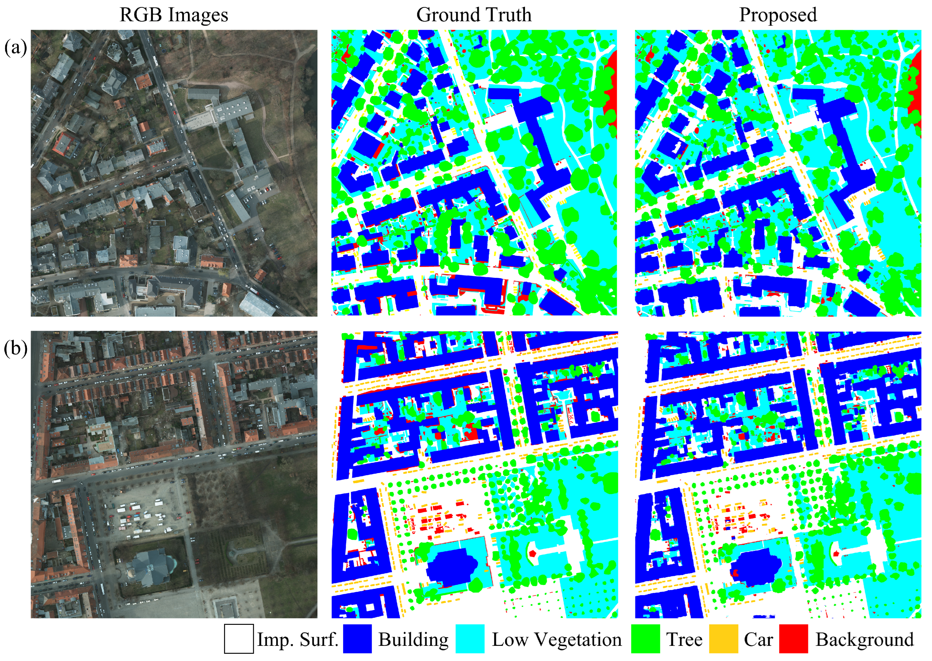
4.4. Experimental Results on the ISPRS Potsdam Dataset

The experimental results of the ISPRS Potsdam dataset are presented in

Table 3. Comparison of semantic segmentation performance on the ISPRS Potsdam dataset between SFA-Net and other segmentation models.

Method	Backbone	Parameters (M)	Imp.surf.	Building	LowVeg	Tree	Car	mF1
DANet [18]	ResNet18	12.6	91.0	95.6	86.1	87.6	84.3	88.9
ABCNet [35]	ResNet18	14.0	93.5	96.9	87.9	89.1	95.8	92.7
Segmenter [24]	Vit-Tiny	6.7	91.5	95.3	85.4	85.0	88.5	89.2
BANet [36]	ResT-Lite	12.7	93.3	96.7	87.4	89.1	96.0	92.5
SwinUperNet [12]	Swin-Tiny	60	93.2	96.4	87.6	88.6	95.4	92.2
DC-Swin [13]	Swin-Small	66.9	94.2	97.6	88.6	89.6	96.3	93.3
UNetFormer [31]	ResNet18	11.7	93.6	97.2	87.7	88.9	96.5	92.8
AerialFormer-B [11]	Swin-Base	113.8	95.5	98.1	89.8	89.8	97.5	94.1
SFA-Net (ours)	EfficientNet-B3	10.7	95.0	97.5	88.3	89.6	97.1	93.5

, and our SFA-Net achieved the second-highest mF1 score with significantly fewer parameters. Specifically, the SFA-Net achieved a 0.6% lower mF1 score compared to the state-of-the-art method AerialFormer-B while reducing 90.59% of the parameters. Among the methods with parameters under 15M, including UNetFormer, BANet, and DANet, the SFA-Net achieved the highest mF1 score of 93.5%. Hybrid models such as SwinUperNet and DC-Swin adopt transformer–CNN architectures for the encoder–decoder and present similar mF1 scores to the SFA-Net. However, they have a significant number of parameters due to the transformer-based backbone, indicating that the CNN–transformer hybrid model is more suitable for efficiency.

Figure 4 shows the entire ID of the test image, ground truth, and prediction data from the ISPRS Potsdam dataset. The ISPRS Potsdam dataset poses a challenge in achieving high segmentation accuracy due to the ‘Background’ and ‘Car’ classes interspersed within the wide region. In the case of the ‘Car’ class, the SFA-Net detects almost every location with an mF1 score of 97.1% despite the small size of the objects. Although the ‘Background’ class is mostly distributed in the small area located between the buildings and other classes, the SFA-Net shows approximate segmentation performance.

We illustrate the qualitative comparison results of the SFA-Net and UNetFormer with ground truth data in Figure 5. As mentioned, the ISPRS Potsdam dataset is challenging due to the ‘Background’ class, so we focused on the performance degradation caused by it. The predictions of UNetFormer, such as (a), (c), and (d), show the incursion of the ‘Background’ class into single-class areas. In contrast, our proposed method significantly minimizes the interference from the ‘Background’ class and predicts more similarly to the ground truth data. In (b), the SFA-Net preserves not only the building edge but also the internal region, leading to accurate building segmentation. These results demonstrate that the SFA-Net has learned semantic information by considering both local and global contexts.

4.5. Experimental Results on the ISPRS Vanihingen Dataset

The experimental results on the ISPRS Vaihingen dataset are presented in

Table 4. Comparison of semantic segmentation performance on the ISPRS Vaihingen dataset between SFA-Net and other segmentation models.

Method	Backbone	Parameters (M)	Imp.surf.	Building	LowVeg	Tree	Car	mF1
DANet [18]	ResNet18	12.6	90.0	93.9	82.2	87.3	44.5	79.6
ABCNet [35]	ResNet18	14.0	92.7	95.2	84.5	89.7	85.3	89.5
BANet [36]	ResT-Lite	12.7	92.2	95.2	83.8	89.9	86.8	89.6
Segmenter [24]	Vit-Tiny	6.7	89.8	93.0	81.2	88.9	67.6	84.1
SwinUperNet [12]	Swin-Tiny	60	92.8	95.6	85.1	90.6	85.1	89.8
DC-Swin [13]	Swin-Small	66.9	93.6	96.2	85.8	90.4	87.6	90.7
UNetFormer [31]	ResNet18	11.7	92.7	95.3	84.9	90.6	88.5	90.4
SFA-Net (ours)	EfficientNet-B3	10.7	93.5	96.3	85.4	90.2	90.7	91.2

, and the SFA-Net achieved the highest performance while maintaining a high level of efficiency. Similar to the results on the ISPRS Potsdam dataset, the SFA-Net shows specialized performance in the ‘Building’ and ‘Car’ classes, with mF1 scores of 96.3% and 90.7%, respectively. Even though SwinUperNet presents the second-highest performance with a well-trained transformer-based encoder, its complexity poses a drawback in terms of efficiency. A segmenter designed with the lowest number of parameters using the Vit-Tiny backbone shows a 7.7% drop in the mF1 score compared to the SFA-Net. In most cases, segmentation accuracy and model efficiency are in a trade-off correlation, and it is important to find the proper balance. We designed the SFA-Net based on this consideration, and the results indicate that our method has achieved a well-balanced performance.

Figure 6 shows the entire ID of the test image, ground truth, and prediction data from the ISPRS Vaihingen dataset. The classes ‘Building’ and ‘Car’ have characteristics of polygon shapes and small sizes over a wide area of observation, respectively. The predicted edges of the ‘Building’ were represented in high quality, with the mF1 score of 96.3%. Consistent with the results from the ISPRS Potsdam dataset, the SFA-Net shows robust detection performance on the ‘Car’ class despite the sparsity of its locations. These results demonstrate that the low-level local features from an efficient CNN-based encoder are enhanced by feature adjustment modules (FAMs).

Figure 7 presents the qualitative results of the SFA-Net and UNetFormer with significant examples. We highlighted the detailed areas in the example data that are complex and easy to confuse. UNetFormer has limitations in terms of accurately classifying the impervious surface (Imp. Surf) area in (a), (b), and (c). In contrast, the SFA-Net shows robust segmentation performance in these local areas while maintaining the natural flow of the semantic features. The SFA-Net utilizes the efficient CNN encoder to enhance the overall efficiency; this may cause the degradation of the local context quality. However, this problem can be solved by adapting a simple refinement module such as FAM, which adjusts the coarse features before analyzing the observation globally.

4.6. Experimental Results on the LoveDA Dataset

Our experimental results on the LoveDA dataset are presented in

Table 5. Comparison of semantic segmentation performance on the LoveDA dataset between SFA-Net and other segmentation models.

Method	Backbone	Parameters (M)	Background	Building	Road	Water	Barren	Forest	Agriculture	mIoU
TransUNet [37]	ResNet50	90.7	43.0	56.1	53.7	78.0	9.3	44.9	56.9	48.9
DC-Swin [13]	Swin-Tiny	66.9	41.3	54.5	56.2	78.1	14.5	47.2	62.4	50.6
UNetFormer [31]	ResNet18	11.7	44.7	58.8	54.9	79.6	20.1	46.0	62.5	52.4
Hi-Resnet [38]	Hi-ResNet	54.3	46.7	58.3	55.9	80.1	17.0	46.7	62.7	52.5
AerialFormer-B [11]	Swin-Base	113.8	47.8	60.7	59.3	81.5	17.9	47.9	64.0	54.1
SFA-Net (ours)	EfficientNet-B3	10.7	48.4	60.3	59.1	81.9	24.1	46.2	64.0	54.9

. The LoveDA dataset poses significant challenges for segmentation due to its complex backgrounds, varying scales of objects, and unbalanced class distribution. The LoveDA dataset does not provide ground truth data for the test set, so we submitted prediction images to the online benchmark platform for the review process. As a result, our proposed method achieved a state-of-the-art mIoU of 54.9%, outperforming AerialFormer-B by 2.5%, while using only 9.41% of its parameters. The SFA-Net outperforms our baseline model UNetFormer in terms of accuracy and efficiency, improving mIoU by 4.55% and reducing the parameters by 8.54%.

Figure 8 presents the qualitative results of UNetFormer and the SFA-Net for the same test set ID, with the key areas highlighted in light gray. Compared to UNetFormer, our method significantly reduces pixel misclassification and predicts the segmentation results close to the actual scene. The SFA-Net distinguishes the ‘Agriculture’ and ‘Water’ classes in (a), including the ground area scene at the center of the lake. Additionally, the SFA-Net accurately predicts the agricultural area in the lower left of (a), whereas UNetFormer predicted it as ‘Barren’. In the highlighted area of (b), UNetFormer confuses between the ‘Building’ and ‘Road’ classes, while our proposed model predicts them correctly. In (c), the SFA-Net shows much clearer segmentation results of the individual buildings compared to UNetFormer, indicating that the SFA-Net has a better understanding of the observations.

4.7. Ablation Study

We conducted an ablation study on feature adjustment modules (FAMs) to demonstrate their effectiveness, and the results are depicted in

Table 6. Ablation study on FAMs. mIoU was measured for the UAVid and LoveDA datasets, and mF1 was measured for the ISPRS Potsdam and ISPRS Vaihingen datasets.

		Dataset
FAM1	FAM2	UAVid	ISPRS Potsdam	ISPRS Vaihingen	LoveDA
		67.8	92.8	90.4	52.4
✓		69.4	93.4	90.5	52.4
	✓	69.7	93.3	90.7	53.1
✓	✓	70.4	93.5	91.2	54.9

. In all the experimented datasets, the segmentation performance gradually elevated with the use of FAMs. In the case of using FAMs individually, FAM2 shows higher performance than FAM1 in almost every dataset except the ISPRS Potsdam dataset. This is an understandable result as we designed FAM1 and FAM2 based on point-wise convolution and fully connected layers, respectively. Since FAM2 refines the high-level features, we adopted a more complex layer than FAM1 to extract a better attention vector. However, FAMs do not significantly increase the overall architecture complexity. Therefore, adopting both FAMs is the best option to obtain high-quality segmentation results.

Table 7. Ablation study on the weight $\alpha$. mIoU was measured for the UAVid and LoveDA datasets, and mF1 was measured for the ISPRS Potsdam and ISPRS Vaihingen datasets.

Dataset	$\mathit{\alpha }$
	0.0	0.2	0.4	0.7	1.0
UAVid	68.4	69.4	70.4	69.9	70.3
ISPRS Potsdam	93.4	93.4	93.5	93.5	93.4
ISPRS Vaihingen	90.7	90.9	91.2	90.9	90.9
LoveDA	52.4	53.4	54.9	53.8	53.4

presents the test results obtained by training with various values of $\alpha$, which weight the auxiliary loss. We designed the auxiliary head in the training process to encourage the intermediate decoder blocks to learn the semantic features. The objective of the auxiliary loss is to minimize the cross-entropy loss between the integrated feature and the ground truth data. As shown in Table 7, our experiment found that 0.4 is the optimal value for $\alpha$ across all datasets.

4.8. Efficiency

We experimented with various CNN-based encoders, including EfficientNet-B0, EfficientNet-B3, ResNet18, and ResNet101, for the encoder of the SFA-Net. In

Table 8. Parameters, FLOPs, and mF1 of each encoder-based segmentation model on the ISPRS Vaihingen dataset.

Dataset	Backbone	Parameters (M)	FLOPs (G)	mF1
ISPRS Vaihingen	EfficientNet-B0	4.2	17.8	87.9
	EfficientNet-B3	10.7	42.8	91.2
	ResNet18	11.9	47.8	90.1
	ResNet101	46.7	186.8	88.5

, we present the number of parameters, FLOPs, and mF1 scores for the encoder-varied SFA-Net on the ISPRS Vaihingen dataset. The EfficientNet-based models show great performance relative to the model complexity compared to the ResNet-based models. Even though the ResNet101-based model has significant model complexity, its segmentation performance drops compared to the ResNet18-based model. Generally, segmentation datasets are small due to the high cost of labeling, which can lead to overfitting in large models.

Table 9. Comparison of parameters and FLOPs between proposed and previous models.

Method	Backbone	Parameters (M)	FLOPs (G)
TransUNet  [37]	ResNet50	90.7	233.7
ABCNet  [35]	ResNet18	14.0	62.9
DC-Swin  [13]	Swin-Tiny	267.8	66.9
UNetFormer  [31]	ResNet18	11.7	46.9
FT-UNetFormer  [31]	Swin-Base	383.9	96.0
AerialFormer-B  [11]	Swin-Base	126.8	-
SFA-Net (ours)	EfficientNet-B3	10.7	42.8

presents a comparison of the number of parameters and FLOPs for the previous and proposed methods. Additionally, we visualized a complexity vs. performance graph of each dataset in Figure 9. The proposed SFA-Net is designed with the lowest complexity by utilizing a hybrid architecture composed of an efficient CNN-based encoder and skip connection modules. Moreover, the SFA-Net is located in the upper left region of all the visualized graphs, indicating that our method achieves high segmentation performance while maintaining lower complexity.

5. Conclusions

In this paper, we propose an efficient hybrid model, the SFA-Net, for the semantic segmentation of remote sensing images. Our method provides high-quality segmentation results by utilizing an efficient CNN-based encoder, a transformer-based decoder, and feature adjustment modules as skip connections. The experimental results demonstrate the high accuracy and efficiency of the SFA-Net in processing complex high-resolution images. In terms of accuracy, we achieved state-of-the-art performance on benchmark datasets, including UAVid, ISPRS Vaihingen, and LoveDA. By comparing the model complexity to the previous methods, we demonstrate the small size and low computational cost of the SFA-Net. We expect the SFA-Net to be applied in a broad range of remote sensing applications that require high-quality segmentation results in real time.

References

1. Mnih, V.; Hinton, G.E. Learning to Detect Roads in High-Resolution Aerial Images. In Computer Vision–ECCV 2010, Proceedings of the 11th European Conference on Computer Vision, Heraklion, Crete, Greece, 5–11 September 2010; Daniilidis, K., Maragos, P., Paragios, N., Eds.; Springer: Berlin/Heidelberg, Germany, 2010; pp. 210–223. [Google Scholar]
2. Demir, I.; Koperski, K.; Lindenbaum, D.; Pang, G.; Huang, J.; Basu, S.; Hughes, F.; Tuia, D.; Raskar, R. DeepGlobe 2018: A Challenge to Parse the Earth Through Satellite Images. In Proceedings of the IEEE Conference on Computer Vision and Pattern Recognition (CVPR) Workshops, Salt Lake City, UT, USA, 18–23 June 2018. [Google Scholar]
3. Mohajerani, S.; Saeedi, P. Cloud-Net: An End-to-End Cloud Detection Algorithm for Landsat 8 Imagery. In Proceedings of the IGARSS 2019—2019 IEEE International Geoscience and Remote Sensing Symposium, Yokohama, Japan, 28 July–2 August 2019; pp. 1029–1032. [Google Scholar] [CrossRef]
4. Maji, S.; Rahtu, E.; Kannala, J.; Blaschko, M.; Vedaldi, A. Fine-Grained Visual Classification of Aircraft. arXiv 2013, arXiv:1306.5151. [Google Scholar]
5. Chen, H.; Shi, Z. A Spatial-Temporal Attention-Based Method and a New Dataset for Remote Sensing Image Change Detection. Remote Sens. 2020, 12, 1662. [Google Scholar] [CrossRef]
6. Zhang, C.; Yue, P.; Tapete, D.; Jiang, L.; Shangguan, B.; Huang, L.; Liu, G. A deeply supervised image fusion network for change detection in high resolution bi-temporal remote sensing images. ISPRS J. Photogramm. Remote Sens. 2020, 166, 183–200. [Google Scholar] [CrossRef]
7. Zhang, Z.; Guo, W.; Zhu, S.; Yu, W. Toward Arbitrary-Oriented Ship Detection With Rotated Region Proposal and Discrimination Networks. IEEE Geosci. Remote Sens. Lett. 2018, 15, 1745–1749. [Google Scholar] [CrossRef]
8. Karra, K.; Kontgis, C.; Statman-Weil, Z.; Mazzariello, J.C.; Mathis, M.; Brumby, S.P. Global land use/land cover with Sentinel 2 and deep learning. In Proceedings of the 2021 IEEE International Geoscience and Remote Sensing Symposium IGARSS, Brussels, Belgium, 11–16 July 2021; pp. 4704–4707. [Google Scholar] [CrossRef]
9. Ma, X.; Zhang, X.; Pun, M.O. RS3Mamba: Visual State Space Model for Remote Sensing Image Semantic Segmentation. IEEE Geosci. Remote Sens. Lett. 2024, 21. [Google Scholar] [CrossRef]
10. Kang, X.; Hong, Y.; Duan, P.; Li, S. Fusion of hierarchical class graphs for remote sensing semantic segmentation. Inf. Fusion 2024, 109, 102409. [Google Scholar] [CrossRef]
11. Yamazaki, K.; Hanyu, T.; Tran, M.; Garcia, A.; Tran, A.; McCann, R.; Liao, H.; Rainwater, C.; Adkins, M.; Molthan, A.; et al. AerialFormer: Multi-resolution Transformer for Aerial Image Segmentation. arXiv 2023, arXiv:2306.06842. [Google Scholar]
12. Liu, Z.; Lin, Y.; Cao, Y.; Hu, H.; Wei, Y.; Zhang, Z.; Lin, S.; Guo, B. Swin transformer: Hierarchical vision transformer using shifted windows. In Proceedings of the IEEE/CVF International Conference on Computer Vision, Montreal, QC, Canada, 10–17 October 2021; pp. 10012–10022. [Google Scholar]
13. Wang, L.; Li, R.; Duan, C.; Zhang, C.; Meng, X.; Fang, S. A Novel Transformer Based Semantic Segmentation Scheme for Fine-Resolution Remote Sensing Images. IEEE Geosci. Remote Sens. Lett. 2022, 19, 1–5. [Google Scholar] [CrossRef]
14. Long, J.; Shelhamer, E.; Darrell, T. Fully convolutional networks for semantic segmentation. In Proceedings of the IEEE Conference on Computer Vision and Pattern Recognition, Boston, MA, USA, 7–12 June 2015; pp. 3431–3440. [Google Scholar]
15. Ronneberger, O.; Fischer, P.; Brox, T. U-Net: Convolutional Networks for Biomedical Image Segmentation. arXiv 2015, arXiv:1505.04597. [Google Scholar]
16. Badrinarayanan, V.; Kendall, A.; Cipolla, R. SegNet: A Deep Convolutional Encoder-Decoder Architecture for Image Segmentation. arXiv 2016, arXiv:1511.00561. [Google Scholar] [CrossRef]
17. Zhao, H.; Shi, J.; Qi, X.; Wang, X.; Jia, J. Pyramid Scene Parsing Network. arXiv 2017, arXiv:1612.01105. [Google Scholar]
18. Fu, J.; Liu, J.; Tian, H.; Li, Y.; Bao, Y.; Fang, Z.; Lu, H. Dual Attention Network for Scene Segmentation. arXiv 2019, arXiv:1809.02983. [Google Scholar]
19. Sun, K.; Zhao, Y.; Jiang, B.; Cheng, T.; Xiao, B.; Liu, D.; Mu, Y.; Wang, X.; Liu, W.; Wang, J. High-Resolution Representations for Labeling Pixels and Regions. arXiv 2019, arXiv:1904.04514. [Google Scholar]
20. Islam, M.A.; Kowal, M.; Jia, S.; Derpanis, K.G.; Bruce, N.D.B. Global Pooling, More than Meets the Eye: Position Information is Encoded Channel-Wise in CNNs. arXiv 2021, arXiv:2108.07884. [Google Scholar]
21. Gu, X.; Li, S.; Ren, S.; Zheng, H.; Fan, C.; Xu, H. Adaptive enhanced swin transformer with U-net for remote sensing image segmentation. Comput. Electr. Eng. 2022, 102, 108223. [Google Scholar] [CrossRef]
22. Vaswani, A.; Shazeer, N.; Parmar, N.; Uszkoreit, J.; Jones, L.; Gomez, A.N.; Kaiser, L.U.; Polosukhin, I. Attention is All you Need. In Advances in Neural Information Processing Systems; Guyon, I., Luxburg, U.V., Bengio, S., Wallach, H., Fergus, R., Vishwanathan, S., Garnett, R., Eds.; Curran Associates, Inc.: Long Beach, CA, USA, 2017; Volume 30. [Google Scholar]
23. Xie, E.; Wang, W.; Yu, Z.; Anandkumar, A.; Alvarez, J.M.; Luo, P. SegFormer: Simple and Efficient Design for Semantic Segmentation with Transformers. In Advances in Neural Information Processing Systems; Ranzato, M., Beygelzimer, A., Dauphin, Y., Liang, P., Vaughan, J.W., Eds.; Curran Associates, Inc.: San Diego, CA, USA, 2021; Volume 34, pp. 12077–12090. [Google Scholar]
24. Strudel, R.; Garcia, R.; Laptev, I.; Schmid, C. Segmenter: Transformer for Semantic Segmentation. In Proceedings of the IEEE/CVF International Conference on Computer Vision (ICCV), Montreal, QC, Canada, 10–17 October 2021; pp. 7262–7272. [Google Scholar]
25. Zhang, C.; Wang, L.; Cheng, S.; Li, Y. SwinSUNet: Pure Transformer Network for Remote Sensing Image Change Detection. IEEE Trans. Geosci. Remote Sens. 2022, 60, 1–13. [Google Scholar] [CrossRef]
26. Liu, M.; Chai, Z.; Deng, H.; Liu, R. A CNN-Transformer Network With Multiscale Context Aggregation for Fine-Grained Cropland Change Detection. IEEE J. Sel. Top. Appl. Earth Obs. Remote Sens. 2022, 15, 4297–4306. [Google Scholar] [CrossRef]
27. Cheng, H.K.; Chung, J.; Tai, Y.W.; Tang, C.K. CascadePSP: Toward Class-Agnostic and Very High-Resolution Segmentation via Global and Local Refinement. arXiv 2020, arXiv:2005.02551. [Google Scholar]
28. Qin, X.; Fan, D.P.; Huang, C.; Diagne, C.; Zhang, Z.; Sant’Anna, A.C.; Suàrez, A.; Jagersand, M.; Shao, L. Boundary-Aware Segmentation Network for Mobile and Web Applications. arXiv 2021, arXiv:2101.04704. [Google Scholar]
29. Dong, Z.; Li, J.; Fang, T.; Shao, X. Lightweight boundary refinement module based on point supervision for semantic segmentation. Image Vis. Comput. 2021, 110, 104169. [Google Scholar] [CrossRef]
30. Tan, M.; Le, Q.V. EfficientNet: Rethinking Model Scaling for Convolutional Neural Networks. arXiv 2020, arXiv:1905.11946. [Google Scholar]
31. Wang, L.; Li, R.; Zhang, C.; Fang, S.; Duan, C.; Meng, X.; Atkinson, P.M. UNetFormer: A UNet-like transformer for efficient semantic segmentation of remote sensing urban scene imagery. ISPRS J. Photogramm. Remote Sens. 2022, 190, 196–214. [Google Scholar] [CrossRef]
32. Lyu, Y.; Vosselman, G.; Xia, G.S.; Yilmaz, A.; Yang, M.Y. UAVid: A semantic segmentation dataset for UAV imagery. ISPRS J. Photogramm. Remote Sens. 2020, 165, 108–119. [Google Scholar] [CrossRef]
33. Potsdam and Vaihingen Datasets. International Society for Photogrammetry and Remote Sensing. Available online: https://www.isprs.org/education/benchmarks/UrbanSemLab (accessed on 20 June 2024).
34. Wang, J.; Zheng, Z.; Ma, A.; Lu, X.; Zhong, Y. LoveDA: A Remote Sensing Land-Cover Dataset for Domain Adaptive Semantic Segmentation. In Neural Information Processing Systems Track on Datasets and Benchmarks; Vanschoren, J., Yeung, S., Eds.; Curran: San Diego, CA, USA, 2021; Volume 1. [Google Scholar]
35. Li, R.; Zheng, S.; Zhang, C.; Duan, C.; Wang, L.; Atkinson, P.M. ABCNet: Attentive bilateral contextual network for efficient semantic segmentation of Fine-Resolution remotely sensed imagery. ISPRS J. Photogramm. Remote Sens. 2021, 181, 84–98. [Google Scholar] [CrossRef]
36. Wang, L.; Li, R.; Wang, D.; Duan, C.; Wang, T.; Meng, X. Transformer meets convolution: A bilateral awareness network for semantic segmentation of very fine resolution urban scene images. Remote Sens. 2021, 13, 3065. [Google Scholar] [CrossRef]
37. Chen, J.; Lu, Y.; Yu, Q.; Luo, X.; Adeli, E.; Wang, Y.; Lu, L.; Yuille, A.L.; Zhou, Y. Transunet: Transformers make strong encoders for medical image segmentation. arXiv 2021, arXiv:2102.04306. [Google Scholar]
38. Chen, Y.; Fang, P.; Yu, J.; Zhong, X.; Zhang, X.; Li, T. Hi-ResNet: A High-Resolution Remote Sensing Network for Semantic Segmentation. arXiv 2023, arXiv:2305.12691. [Google Scholar]
Figure 1. The overall architecture of the SFA-Net.
Remotesensing 16 03278 g001
Figure 2. Transformer-based decoder. (ac) present the decoder block, weighted function, and feature refinement head, respectively.
Remotesensing 16 03278 g002
Figure 3. Visualization of the segmentation results on the UAVid datasets. (a) is ID 000300 in sequence 23, (b) is ID 000500 in sequence 28, (c) is ID 000000 id in sequence 30, and (d) is ID 000500 id in sequence 39.
Remotesensing 16 03278 g003
Figure 4. Visualization of the entire set of IDs and their segmentation results on the ISPRS Potsdam dataset. (a) is ID 3_14 and (b) is ID 5_13.
Remotesensing 16 03278 g004
Figure 5. Visualization of the segmentation results on the ISPRS Potsdam dataset. (a) is the 10th split of ID 3_14, (b) is the 12th split of ID 5_13, (c) is the 10th split of ID 6_14, and (d) is the 22nd split of ID 7_13.
Remotesensing 16 03278 g005
Figure 6. Visualization of the entire set of IDs and their segmentation results on the ISPRS Vaihingen test datasets. (a) is area 6 and (b) is area 27.
Remotesensing 16 03278 g006
Figure 7. Visualization of the segmentation results on the ISPRS Vaihingen dataset. (a) is the 4th split of ID area 31, and (b) is the 5th split from 2nd of area 33. (c) is the 4th split of area 38, and (d) is the 11th split of area 38.
Remotesensing 16 03278 g007
Figure 8. Visualization of the segmentation results on the LoveDA dataset. (a) is 4430, (b) is 4378, and (c) is 5458.
Remotesensing 16 03278 g008
Figure 9. Visualized complexity vs. performance graph of each dataset. The horizontal and vertical axes denote FLOPs and evaluation metrics, respectively, and the bubble diameter denotes the number of parameters.
Remotesensing 16 03278 g009