
Combination of Multiple Variables and Machine Learning for Regional Cropland Water and Carbon Fluxes Estimation: A Case Study in the Haihe River Basin


Abstract
:1. Introduction
2. Study Area and Data Collection
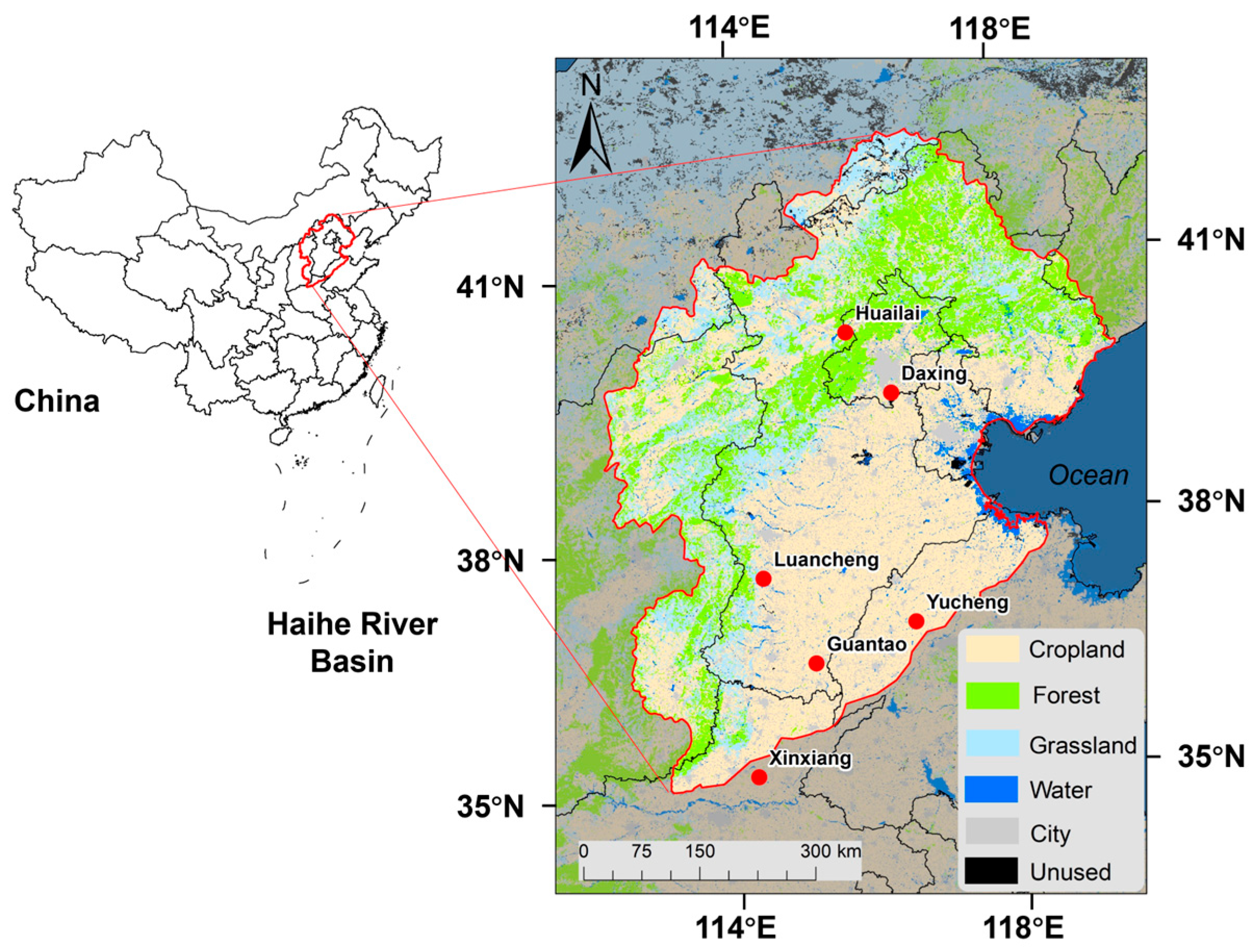
2.1. Study Area
2.2. Satellite Data
2.3. Flux Data
3. Methodology
3.1. Machine Learning Methods
- (1)
- Random forest regression (RFR)
- Random Sampling—Using the bootstrap sampling method to randomly extract multiple sample sets from the original training data set, with each sample set having the same size as the original data set;
- Decision Tree Construction—For each sample set, construct a decision tree. During the tree construction process, introduce randomness to increase the diversity of the trees, such as randomly selecting features for splitting;
- Each decision tree independently predicts new data;
- Ensemble Prediction—Averaging the prediction results of all decision trees to obtain the final prediction result.
- (2)
- Backpropagation Neural Network (BPNN)
- Network Initialization—Randomly set the weights and biases between neurons in each layer;
- Forward Propagation of Input Signals—Propagate the input signals forward through the network and calculate the output of neurons in each layer;
- Error Calculation—Calculate the error based on the network’s output and the desired output;
- Error Backpropagation—Propagate the error signal backward and adjust the weights and biases of neurons in each layer according to the gradient descent method or other optimization algorithms;
- Iterative Training—Repeat steps b to d until the maximum number of iterations.
3.2. Input Variables
- (1)
- Vegetation growth
- (2)
- Surface moisture
- (3)
- Radiation energy
- (4)
- Others
3.3. Modeling and Validation
3.3.1. Modeling Methods
3.3.2. Validation Methods
4. Results
4.1. Modeling and Validation of ET and NEE Estimation
4.1.1. Contributions of Different Input Variables
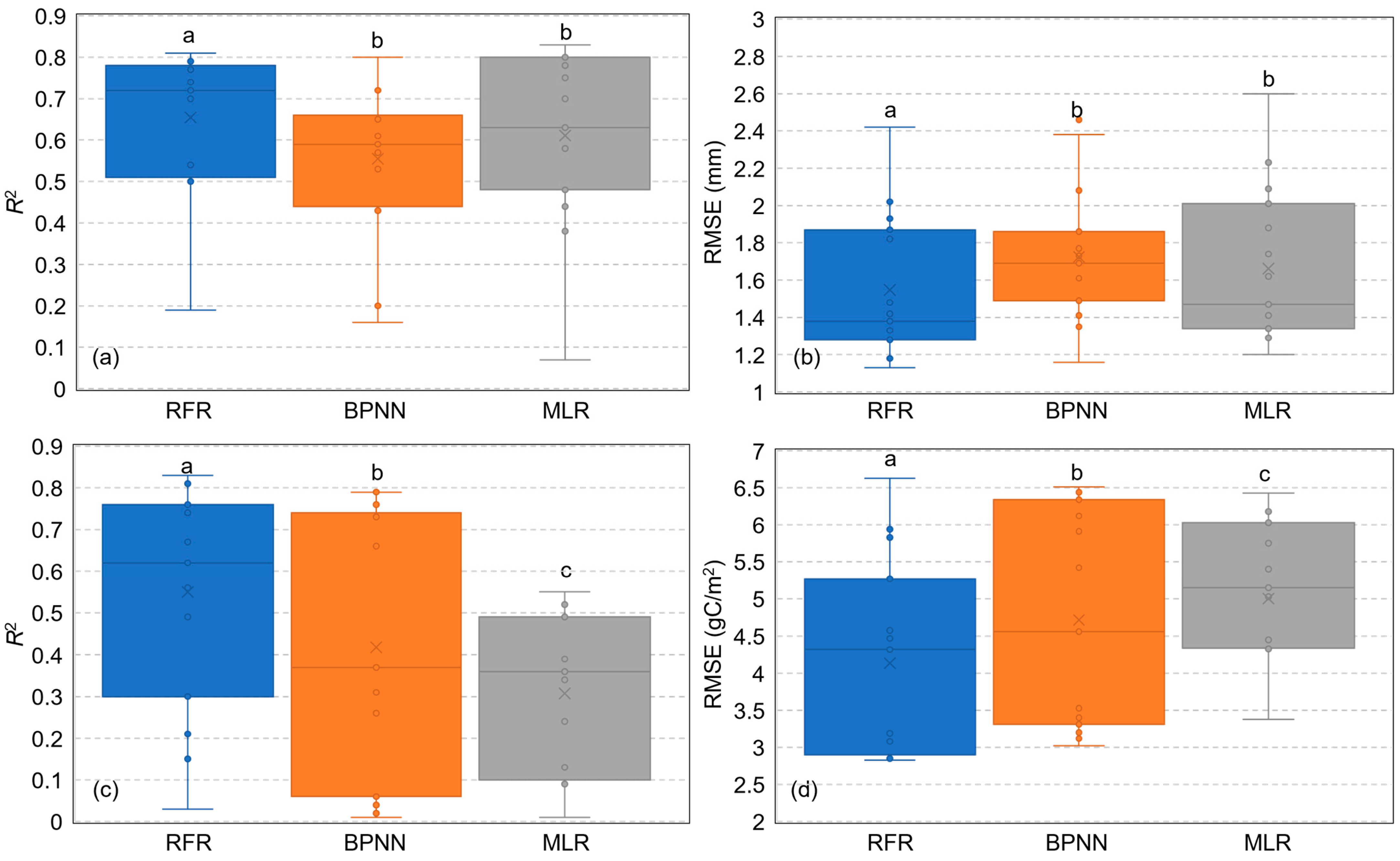
4.1.2. The Performance of Different Regression Methods
4.1.3. The Stability of the Model in Different Sites
4.2. Spatial Distribution
5. Discussion
6. Conclusions
- (1)
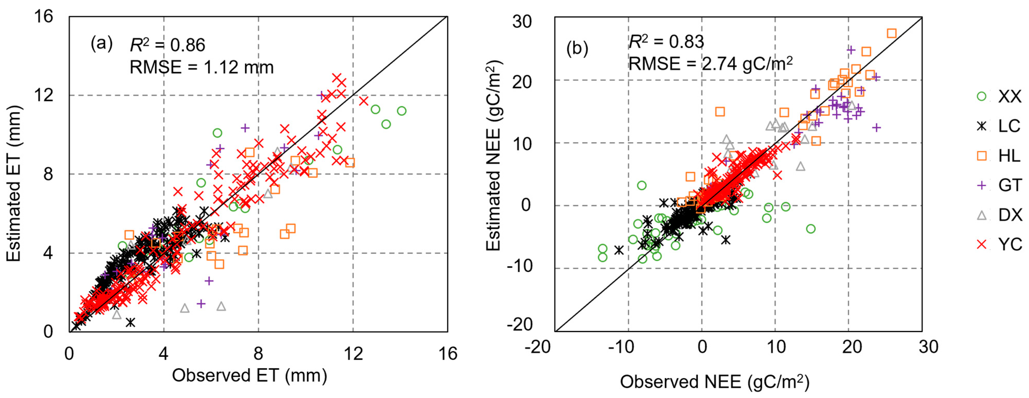
- Increasing the number of input variables typically improved the accuracy of ET and NEE estimations. Here, four types of variables used together (RFR) resulted in the best accuracy for ET (R2 of 0.81 and an RMSE of 1.13 mm) and NEE (R2 of 0.83 and an RMSE of 2.83 gC/m2) estimations. Moreover, vegetation growth variables (i.e., VIs) are the most important inputs for ET and NEE estimation;
- (2)
- Among the three regression algorithms tested, each demonstrated different levels of accuracy in estimating ET and NEE. Overall, RFR proved to be the most accurate for both ET and NEE estimations;
- (3)
- The proposed ET and NEE estimation models exhibited some variation in accuracy across different validation sites. Specifically, the R2 for ET estimation ranged from 0.51 to 0.87, and the RMSE fluctuated between 0.94 and 2.28 mm across the six sites. Similarly, for NEE estimation, the R2 spanned from 0.35 to 0.80, with the RMSE varying from 1.42 to 5.48 gC/m2. Despite these variations, the accuracy levels across all six validation sites remained relatively high.
Author Contributions
Funding
Data Availability Statement
Conflicts of Interest
References
- Wang, S.; Garcia, M.; Bauer-Gottwein, P.; Jakobsen, J.; Zarco-Tejada, P.J.; Bandini, F.; Paz, V.S.; Ibrom, A. High spatial resolution monitoring land surface energy, water and CO2 fluxes from an Unmanned Aerial System. Remote Sens. Environ. 2019, 229, 14–31. [Google Scholar] [CrossRef]
- Cheng, M.; Jiao, X.; Jin, X.; Li, B.; Liu, K.; Shi, L. Satellite time series data reveal interannual and seasonal spatiotemporal evapotranspiration patterns in China in response to effect factors. Agric. Water Manag. 2021, 255, 107046. [Google Scholar] [CrossRef]
- Heimann, M.; Reichstein, M. Terrestrial ecosystem carbon dynamics and climate feedbacks. Nature 2008, 451, 289–292. [Google Scholar] [CrossRef] [PubMed]
- Cheng, M.; Jiao, X.; Liu, Y.; Shao, M.; Yu, X.; Bai, Y.; Wang, Z.; Wang, S.; Tuohuti, N.; Liu, S. Estimation of soil moisture content under high maize canopy coverage from UAV multimodal data and machine learning. Agric. Water Manag. 2022, 264, 107530. [Google Scholar] [CrossRef]
- Ezzahar, J.; Chehbouni, A.; Hoedjes, J.C.; Er-Raki, S.; Chehbouni, A.; Boulet, G.; Bonnefond, J.-M.; De Bruin, H. The use of the scintillation technique for monitoring seasonal water consumption of olive orchards in a semi-arid region. Agric. Water Manag. 2007, 89, 173–184. [Google Scholar] [CrossRef]
- Bastiaanssen, W.G.; Menenti, M.; Feddes, R.; Holtslag, A. A remote sensing surface energy balance algorithm for land (SEBAL).: Part 1. Formulation. J. Hydrol. 1998, 212, 198–212. [Google Scholar] [CrossRef]
- Bastiaanssen, W.G.; Pelgrum, H.; Wang, J.; Ma, Y.; Moreno, J.; Roerink, G.; Van der Wal, T. A remote sensing surface energy balance algorithm for land (SEBAL).: Part 2: Validation. J. Hydrol. 1998, 212, 213–229. [Google Scholar] [CrossRef]
- Anderson, M.; Norman, J.; Diak, G.; Kustas, W.; Mecikalski, J. A two-source time-integrated model for estimating surface fluxes using thermal infrared remote sensing. Remote Sens. Environ. 1997, 60, 195–216. [Google Scholar] [CrossRef]
- Su, Z. The Surface Energy Balance System (SEBS) for estimation of turbulent heat fluxes. Hydrol. Earth Syst. Sci. 2002, 6, 85–99. [Google Scholar] [CrossRef]
- Awada, H.; Di Prima, S.; Sirca, C.; Giadrossich, F.; Marras, S.; Spano, D.; Pirastru, M. A remote sensing and modeling integrated approach for constructing continuous time series of daily actual evapotranspiration. Agric. Water Manag. 2022, 260, 107320. [Google Scholar] [CrossRef]
- Laipelt, L.; Bloedow Kayser, R.H.; Fleischmann, A.S.; Ruhoff, A.; Bastiaanssen, W.; Erickson, T.A.; Melton, F. Long-term monitoring of evapotranspiration using the SEBAL algorithm and Google Earth Engine cloud computing. ISPRS J. Photogramm. Remote Sens. 2021, 178, 81–96. [Google Scholar] [CrossRef]
- Peddinti, S.R.; Kisekka, I. Estimation of turbulent fluxes over almond orchards using high-resolution aerial imagery with one and two-source energy balance models. Agric. Water Manag. 2022, 269, 107671. [Google Scholar] [CrossRef]
- Wolff, W.; Francisco, J.P.; Flumignan, D.L.; Marin, F.R.; Folegatti, M.V. Optimized algorithm for evapotranspiration retrieval via remote sensing. Agric. Water Manag. 2022, 262, 107390. [Google Scholar] [CrossRef]
- Xue, J.; Fulton, A.; Kisekka, I. Evaluating the role of remote sensing-based energy balance models in improving site-specific irrigation management for young walnut orchards. Agric. Water Manag. 2021, 256, 107132. [Google Scholar] [CrossRef]
- Dong, J.; Li, L.; Li, Y.; Yu, Q. Inter-comparisons of mean, trend and interannual variability of global terrestrial gross primary production retrieved from remote sensing approach. Sci. Total Environ. 2022, 822, 153343. [Google Scholar] [CrossRef]
- Guo, H.; Li, S.; Kang, S.; Du, T.; Liu, W.; Tong, L.; Hao, X.; Ding, R. Comparison of several models for estimating gross primary production of drip-irrigated maize in arid regions. Ecol. Model. 2022, 468, 109928. [Google Scholar] [CrossRef]
- Shu, Y.; Liu, S.; Wang, Z.; Xiao, J.; Shi, Y.; Peng, X.; Gao, H.; Wang, Y.; Yuan, W.; Yan, W.; et al. Effects of Aerosols on Gross Primary Production from Ecosystems to the Globe. Remote Sens. 2022, 14, 2759. [Google Scholar] [CrossRef]
- Xiao, F.; Liu, Q.; Xu, Y. Estimation of Terrestrial Net Primary Productivity in the Yellow River Basin of China Using Light Use Efficiency Model. Sustainability 2022, 14, 7399. [Google Scholar] [CrossRef]
- Zhang, Z.; Li, X.; Ju, W.; Zhou, Y.; Cheng, X. Improved estimation of global gross primary productivity during 1981–2020 using the optimized P model. Sci. Total Environ. 2022, 838, 156172. [Google Scholar] [CrossRef]
- Pei, Y.; Dong, J.; Zhang, Y.; Yuan, W.; Doughty, R.; Yang, J.; Zhou, D.; Zhang, L.; Xiao, X. Evolution of light use efficiency models: Improvement, uncertainties, and implications. Agric. For. Meteorol. 2022, 317, 108905. [Google Scholar] [CrossRef]
- Cheng, M.; Jiao, X.; Li, B.; Yu, X.; Shao, M.; Jin, X. Long time series of daily evapotranspiration in China based on the SEBAL model and multisource images and validation. Earth Syst. Sci. Data 2021, 13, 3995–4017. [Google Scholar] [CrossRef]
- Dechant, B.; Ryu, Y.; Badgley, G.; Kohler, P.; Rascher, U.; Migliavacca, M.; Zhang, Y.; Tagliabue, G.; Guan, K.; Rossini, M.; et al. NIRvP: A robust structural proxy for sun-induced chlorophyll fluorescence and photosynthesis across scales. Remote Sens. Environ. 2022, 268, 112763. [Google Scholar] [CrossRef]
- Camps-Valls, G.; Campos-Taberner, M.; Moreno-Martinez, A.; Walther, S.; Duveiller, G.; Cescatti, A.; Mahecha, M.D.; Munoz-Mari, J.; Javier Garcia-Haro, F.; Guanter, L.; et al. A unified vegetation index for quantifying the terrestrial biosphere. Sci. Adv. 2021, 7, eabc7447. [Google Scholar] [CrossRef]
- Dou, X.; Yang, Y. Evapotranspiration estimation using four different machine learning approaches in different terrestrial ecosystems. Comput. Electron. Agric. 2018, 148, 95–106. [Google Scholar] [CrossRef]
- Carter, C.; Liang, S. Evaluation of ten machine learning methods for estimating terrestrial evapotranspiration from remote sensing. Int. J. Appl. Earth Obs. Geoinf. 2019, 78, 86–92. [Google Scholar] [CrossRef]
- Lees, K.J.; Quaife, T.; Artz, R.R.E.; Khomik, M.; Clark, J.M. Potential for using remote sensing to estimate carbon fluxes across northern peatlands—A review. Sci. Total Environ. 2018, 615, 857–874. [Google Scholar] [CrossRef] [PubMed]
- Cheng, M.; Li, B.; Jiao, X.; Huang, X.; Fan, H.; Lin, R.; Liu, K. Using multimodal remote sensing data to estimate regional-scale soil moisture content: A case study of Beijing, China. Agric. Water Manag. 2022, 260, 107298. [Google Scholar] [CrossRef]
- Mu, Q.; Heinsch, F.A.; Zhao, M.; Running, S.W. Development of a global evapotranspiration algorithm based on MODIS and global meteorology data. Remote Sens. Environ. 2007, 111, 519–536. [Google Scholar] [CrossRef]
- Mu, Q.; Zhao, M.; Running, S.W. Improvements to a MODIS global terrestrial evapotranspiration algorithm. Remote Sens. Environ. 2011, 115, 1781–1800. [Google Scholar] [CrossRef]
- Miralles, D.G.; Holmes, T.; De Jeu, R.; Gash, J.; Meesters, A.; Dolman, A. Global land-surface evaporation estimated from satellite-based observations. Hydrol. Earth Syst. Sci. 2011, 15, 453–469. [Google Scholar] [CrossRef]
- Sun, P.; Wu, Y.; Xiao, J.; Hui, J.; Hu, J.; Zhao, F.; Qiu, L.; Liu, S. Remote sensing and modeling fusion for investigating the ecosystem water-carbon coupling processes. Sci. Total Environ. 2019, 697, 134064. [Google Scholar] [CrossRef] [PubMed]
- Gago, J.; Daloso, D.d.M.; Figueroa, C.M.; Flexas, J.; Fernie, A.R.; Nikoloski, Z. Relationships of Leaf Net Photosynthesis, Stomatal Conductance, and Mesophyll Conductance to Primary Metabolism: A Multispecies Meta-Analysis Approach. Plant Physiol. 2016, 171, 265–279. [Google Scholar] [CrossRef] [PubMed]
- Orchard, V.A.; Cook, F. Relationship between soil respiration and soil moisture. Soil Biol. Biochem. 1983, 15, 447–453. [Google Scholar] [CrossRef]
- Kuzyakov, Y.; Domanski, G. Carbon input by plants into the soil. Review. J. Plant Nutr. Soil Sci. 2000, 163, 421–431. [Google Scholar] [CrossRef]
- Murray, S.J.; Foster, P.N.; Prentice, I.C. Evaluation of global continental hydrology as simulated by the Land-surface Processes and eXchanges Dynamic Global Vegetation Model. Hydrol. Earth Syst. Sci. 2011, 15, 91–105. [Google Scholar] [CrossRef]
- Gorelick, N.; Hancher, M.; Dixon, M.; Ilyushchenko, S.; Thau, D.; Moore, R. Google Earth Engine: Planetary-scale geospatial analysis for everyone. Remote Sens. Environ. 2017, 202, 18–27. [Google Scholar] [CrossRef]
- Hansen, M.C.; Potapov, P.V.; Moore, R.; Hancher, M.; Turubanova, S.A.; Tyukavina, A.; Thau, D.; Stehman, S.V.; Goetz, S.J.; Loveland, T.R. High-resolution global maps of 21st-century forest cover change. Science 2013, 342, 850–853. [Google Scholar] [CrossRef]
- Pekel, J.-F.; Cottam, A.; Gorelick, N.; Belward, A.S.J.N. High-resolution mapping of global surface water and its long-term changes. Nature 2016, 540, 418–422. [Google Scholar] [CrossRef]
- Zhang, Y.; Du, J.; Guo, L.; Fang, S.; Zhang, J.; Sun, B.; Mao, J.; Sheng, Z.; Li, L. Long-term detection and spatiotemporal variation analysis of open-surface water bodies in the Yellow River Basin from 1986 to 2020. Sci. Total Environ. 2022, 845, 157152. [Google Scholar] [CrossRef]
- Gumma, M.K.; Thenkabail, P.S.; Panjala, P.; Teluguntla, P.; Yamano, T.; Mohammed, I. Multiple agricultural cropland products of South Asia developed using Landsat-8 30 m and MODIS 250 m data using machine learning on the Google Earth Engine (GEE) cloud and spectral matching techniques (SMTs) in support of food and water security. Giscience Remote Sens. 2022, 59, 1048–1077. [Google Scholar] [CrossRef]
- Cao, J.; Zhang, Z.; Tao, F.; Zhang, L.; Luo, Y.; Zhang, J.; Han, J.; Xie, J. Integrating Multi-Source Data for Rice Yield Prediction across China using Machine Learning and Deep Learning Approaches. Agric. For. Meteorol. 2021, 297, 108275. [Google Scholar] [CrossRef]
- Cao, J.; Zhang, Z.; Luo, Y.; Zhang, L.; Zhang, J.; Li, Z.; Tao, F. Wheat yield predictions at a county and field scale with deep learning, machine learning, and google earth engine. Eur. J. Agron. 2021, 123, 126204. [Google Scholar] [CrossRef]
- Chen, Y.; Xia, J.; Liang, S.; Feng, J.; Fisher, J.B.; Li, X.; Li, X.; Liu, S.; Ma, Z.; Miyata, A.; et al. Comparison of satellite-based evapotranspiration models over terrestrial ecosystems in China. Remote Sens. Environ. 2014, 140, 279–293. [Google Scholar] [CrossRef]
- Jin, X.; Li, Z.; Feng, H.; Ren, Z.; Li, S. Deep neural network algorithm for estimating maize biomass based on simulated Sentinel 2A vegetation indices and leaf area index. Crop J. 2020, 8, 87–97. [Google Scholar] [CrossRef]
- Cheng, M.; Penuelas, J.; McCabe, M.F.; Atzberger, C.; Jiao, X.; Wu, W.; Jin, X. Combining multi-indicators with machine-learning algorithms for maize yield early prediction at the county-level in China. Agric. For. Meteorol. 2022, 323, 109057. [Google Scholar] [CrossRef]
- Maimaitijiang, M.; Sagan, V.; Sidike, P.; Hartling, S.; Fritschi, F.B. Soybean yield prediction from UAV using multimodal data fusion and deep learning. Remote Sens. Environ. 2020, 237, 111599. [Google Scholar] [CrossRef]
- Liu, S.B.; Jin, X.L.; Nie, C.W.; Wang, S.Y.; Yu, X.; Cheng, M.H.; Shao, M.C.; Wang, Z.X.; Tuohuti, N.; Bai, Y.; et al. Estimating leaf area index using unmanned aerial vehicle data: Shallow vs. deep machine learning algorithms. Plant Physiol. 2021, 187, 1551–1576. [Google Scholar] [CrossRef]
- Yu, D.; Zha, Y.; Sun, Z.; Li, J.; Jin, X.; Zhu, W.; Bian, J.; Ma, L.; Zeng, Y.; Su, Z. Deep convolutional neural networks for estimating maize above-ground biomass using multi-source UAV images: A comparison with traditional machine learning algorithms. Precis. Agric. 2022, 24, 92–113. [Google Scholar] [CrossRef]
- Wang, X.; Zhang, F.; Kung, H.-t.; Johnson, V.C. New methods for improving the remote sensing estimation of soil organic matter content (SOMC) in the Ebinur Lake Wetland National Nature Reserve (ELWNNR) in northwest China. Remote Sens. Environ. 2018, 218, 104–118. [Google Scholar] [CrossRef]
- Gobron, N.; Pinty, B.; Verstraete, M.M.; Widlowski, J.L. Advanced vegetation indices optimized for up-coming sensors: Design, performance, and applications. IEEE Trans. Geosci. Remote Sens. 2000, 38, 2489–2505. [Google Scholar]
- Ranjan, R.; Chopra, U.K.; Sahoo, R.N.; Singh, A.K.; Pradhan, S. Assessment of plant nitrogen stress in wheat (Triticum aestivum L.) through hyperspectral indices. Int. J. Remote Sens. 2012, 33, 6342–6360. [Google Scholar] [CrossRef]
- Bajgain, R.; Xiao, X.; Wagle, P.; Basara, J.; Zhou, Y. Sensitivity analysis of vegetation indices to drought over two tallgrass prairie sites. ISPRS J. Photogramm. Remote Sens. 2015, 108, 151–160. [Google Scholar] [CrossRef]
- Huete, A.R. A soil-adjusted vegetation index (SAVI). Remote Sens. Environ. 1988, 25, 295–309. [Google Scholar] [CrossRef]
- Dong, T.; Liu, J.; Qian, B.; Zhao, T.; Jing, Q.; Geng, X.; Wang, J.; Huffman, T.; Shang, J. Estimating winter wheat biomass by assimilating leaf area index derived from fusion of Landsat-8 and MODIS data. Int. J. Appl. Earth Obs. Geoinf. 2016, 49, 63–74. [Google Scholar] [CrossRef]
- Chen, H.; Zhao, G.; Li, Y.; Wang, D.; Ma, Y. Monitoring the seasonal dynamics of soil salinization in the Yellow River delta of China using Landsat data. Nat. Hazards Earth Syst. Sci. 2019, 19, 1499–1508. [Google Scholar] [CrossRef]
- Vincini, M.; Frazzi, E.; D’Alessio, P. A broad-band leaf chlorophyll vegetation index at the canopy scale. Precis. Agric. 2008, 9, 303–319. [Google Scholar] [CrossRef]
- Gilbertson, J.K.; Kemp, J.; van Niekerk, A. Effect of pan-sharpening multi-temporal Landsat 8 imagery for crop type differentiation using different classification techniques. Comput. Electron. Agric. 2017, 134, 151–159. [Google Scholar] [CrossRef]
- Tang, Z.; Li, Y.; Gu, Y.; Jiang, W.; Xue, Y.; Hu, Q.; LaGrange, T.; Bishop, A.; Drahota, J.; Li, R. Assessing Nebraska playa wetland inundation status during 1985–2015 using Landsat data and Google Earth Engine. Environ. Monit. Assess. 2016, 188, 654. [Google Scholar] [CrossRef]
- Morton, D.C.; DeFries, R.S.; Nagol, J.; Souza, C.M., Jr.; Kasischke, E.S.; Hurtt, G.C.; Dubayah, R. Mapping canopy damage from understory fires in Amazon forests using annual time series of Landsat and MODIS data. Remote Sens. Environ. 2011, 115, 1706–1720. [Google Scholar] [CrossRef]
- Balogun, A.-L.; Yekeen, S.T.; Pradhan, B.; Althuwaynee, O.F. Spatio-Temporal Analysis of Oil Spill Impact and Recovery Pattern of Coastal Vegetation and Wetland Using Multispectral Satellite Landsat 8-OLI Imagery and Machine Learning Models. Remote Sens. 2020, 12, 1225. [Google Scholar] [CrossRef]
- Sandholt, I.; Rasmussen, K.; Andersen, J. A simple interpretation of the surface temperature/vegetation index space for assessment of surface moisture status. Remote Sens. Environ. 2002, 79, 213–224. [Google Scholar] [CrossRef]
- Fang, S.; Mao, K.; Xia, X.; Wang, P.; Shi, J.; Bateni, S.M.; Xu, T.; Cao, M.; Heggy, E.; Qin, Z. Dataset of daily near-surface air temperature in China from 1979 to 2018. Earth Syst. Sci. Data 2022, 14, 1413–1432. [Google Scholar] [CrossRef]
- Damm, A.; Paul-Limoges, E.; Kukenbrink, D.; Bachofen, C.; Morsdorf, F. Remote sensing of forest gas exchange: Considerations derived from a tomographic perspective. Glob. Chang. Biol. 2020, 26, 2717–2727. [Google Scholar] [CrossRef] [PubMed]
- Kljun, N.; Calanca, P.; Rotach, M.; Schmid, H. The simple two-dimensional parameterisation for Flux Footprint Predictions FFP. Geosci. Model Dev. Discuss. 2015, 8, 3695–3713. [Google Scholar] [CrossRef]
- Rudiger, C.; Su, C.H.; Ryu, D.; Wagner, W. Disaggregation of Low-Resolution L-Band Radiometry Using C-Band Radar Data. IEEE Geosci. Remote Sens. Lett. 2016, 13, 1425–1429. [Google Scholar] [CrossRef]
- Wang, W.; Cui, W.; Wang, X.J.; Chen, X. Evaluation of GLDAS-1 and GLDAS-2 Forcing Data and Noah Model Simulations over China at the Monthly Scale. J. Hydrometeorol. 2016, 17, 2815–2833. [Google Scholar] [CrossRef]
- Ji, L.; Senay, G.B.; Verdin, J.P. Evaluation of the Global Land Data Assimilation System (GLDAS) Air Temperature Data Products. J. Hydrometeorol. 2015, 16, 2463–2480. [Google Scholar] [CrossRef]
- Du, Y.F.; Shi, H.R.; Zhang, J.Q.; Xia, X.A.; Yao, Z.D.; Fu, D.S.; Hu, B.; Huang, C.L. Evaluation of MERRA-2 hourly surface solar radiation across China. Sol. Energy 2022, 234, 103–110. [Google Scholar] [CrossRef]
- Hancox-Li, L. Robustness in machine learning explanations: Does it matter? In Proceedings of the 2020 Conference on Fairness, Accountability, and Transparency, Barcelona, Spain, 27–30 January 2020; pp. 640–647. [Google Scholar]
- Zhou, J.; Gandomi, A.H.; Chen, F.; Holzinger, A. Evaluating the Quality of Machine Learning Explanations: A Survey on Methods and Metrics. Electronics 2021, 10, 593. [Google Scholar] [CrossRef]
- Webb, G.I.; Zheng, Z.J. Multistrategy ensemble learning: Reducing error by combining ensemble learning techniques. IEEE Trans. Knowl. Data Eng. 2004, 16, 980–991. [Google Scholar] [CrossRef]
- Sheykhmousa, M.; Mahdianpari, M.; Ghanbari, H.; Mohammadimanesh, F.; Ghamisi, P.; Homayouni, S. Support Vector Machine Versus Random Forest for Remote Sensing Image Classification: A Meta-Analysis and Systematic Review. IEEE J. Sel. Top. Appl. Earth Obs. Remote Sens. 2020, 13, 6308–6325. [Google Scholar] [CrossRef]
- He, L.; Ren, X.; Wang, Y.; Liu, B.; Zhang, H.; Liu, W.; Feng, W.; Guo, T. Comparing methods for estimating leaf area index by multi-angular remote sensing in winter wheat. Sci. Rep. 2020, 10, 13943. [Google Scholar] [CrossRef] [PubMed]
- Ilori, C.O.; Pahlevan, N.; Knudby, A. Analyzing performances of different atmospheric correction techniques for Landsat 8: Application for coastal remote sensing. Remote Sens. 2019, 11, 469. [Google Scholar] [CrossRef]
- Chander, G.; Markham, B.L.; Helder, D.L. Summary of current radiometric calibration coefficients for Landsat MSS, TM, ETM+, and EO-1 ALI sensors. Remote Sens. Environ. 2009, 113, 893–903. [Google Scholar] [CrossRef]
- Wang, K.; Dickinson, R.E. A review of global terrestrial evapotranspiration: Observation, modeling, climatology, and climatic variability. Rev. Geophys. 2012, 50. [Google Scholar] [CrossRef]
- Vickers, D.; Gockede, M.; Law, B.E. Uncertainty estimates for 1-h averaged turbulence fluxes of carbon dioxide, latent heat and sensible heat. Tellus Ser. B-Chem. Phys. Meteorol. 2010, 62, 87–99. [Google Scholar] [CrossRef]
- Foken, T. The energy balance closure problem: An overview. Ecol. Appl. 2008, 18, 1351–1367. [Google Scholar] [CrossRef] [PubMed]
- Liu, Z. The accuracy of temporal upscaling of instantaneous evapotranspiration to daily values with seven upscaling methods. Hydrol. Earth Syst. Sci. 2021, 25, 4417–4433. [Google Scholar] [CrossRef]
- Vancutsem, C.; Ceccato, P.; Dinku, T.; Connor, S.J. Evaluation of MODIS land surface temperature data to estimate air temperature in different ecosystems over Africa. Remote Sens. Environ. 2010, 114, 449–465. [Google Scholar] [CrossRef]
- Phan Thanh, N.; Kappas, M.; Degener, J. Estimating Daily Maximum and Minimum Land Air Surface Temperature Using MODIS Land Surface Temperature Data and Ground Truth Data in Northern Vietnam. Remote Sens. 2016, 8, 2. [Google Scholar] [CrossRef]
- Zhang, H.; Zhang, F.; Zhang, G.; Ma, Y.; Yang, K.; Ye, M. Daily air temperature estimation on glacier surfaces in the Tibetan Plateau using MODIS LST data. J. Glaciol. 2018, 64, 132–147. [Google Scholar] [CrossRef]
- Zhu, W.; Lű, A.; Jia, S. Estimation of daily maximum and minimum air temperature using MODIS land surface temperature products. Remote Sens. Environ. 2013, 130, 62–73. [Google Scholar] [CrossRef]


| Dataset | Bands ID | Wavelength | Description | Temporal/Spatial Resolution |
|---|---|---|---|---|
| Landsat 7 Level 2, Collection 2, Tier 1 | SR_B1 | 0.452–0.512 μm | blue surface reflectance | 16 day/30 m |
| SR_B2 | 0.533–0.590 μm | green surface reflectance | 16 day/30 m | |
| SR_B3 | 0.636–0.673 μm | red surface reflectance | 16 day/30 m | |
| SR_B4 | 0.851–0.879 μm | near infrared surface reflectance | 16 day/30 m | |
| SR_B5 | 1.566–1.651 μm | shortwave infrared 1 surface reflectance | 16 day/30 m | |
| ST_B6 | 10.40–12.50 μm | surface temperature (K) | 16 day/30 m (resampled from 100 m) | |
| SR_B7 | 2.107–2.294 μm | shortwave infrared 2 surface reflectance | 16 day/30 m | |
| Landsat 8 Level 2, Collection 2, Tier 1 | SR_B2 | 0.452–0.512 μm | blue surface reflectance | 16 day/30 m |
| SR_B3 | 0.533–0.590 μm | green surface reflectance | 16 day/30 m | |
| SR_B4 | 0.636–0.673 μm | red surface reflectance | 16 day/30 m | |
| SR_B5 | 0.851–0.879 μm | near infrared surface reflectance | 16 day/30 m | |
| SR_B6 | 1.566–1.651 μm | shortwave infrared 1 surface reflectance | 16 day/30 m | |
| SR_B7 | 2.107–2.294 μm | shortwave infrared 2 surface reflectance | 16 day/30 m | |
| ST_B10 | 10.60–11.19 μm | surface temperature (K) | 16 day/30 m (resampled from 100 m) |
| Site Name | Observation Period | Longitude | Latitude | Elevation | Surface Types |
|---|---|---|---|---|---|
| Daxing (DXC) | 2008–2010 | 116.43° | 39.62° | 20 m | Maize/wheat |
| Guantao (GTC) | 2008–2010 | 115.13° | 36.52° | 30 m | Maize/wheat |
| Huailai (HL) | 2016–2017 | 115.79° | 40.35° | 480 m | Maize/wheat |
| Luancheng (LC) | 2007–2018 | 114.41° | 37.53° | 50 m | Maize/wheat |
| Yucheng (YC) | 2003–2010 | 116.60° | 36.95° | 28 m | Maize/wheat |
| Xinxiang (XX) | 2019–2020 | 114.25° | 35.22° | 74 m | Maize/wheat |
| Algorithms | Main Parameters |
|---|---|
| Random Forest | n_estimators = 20, max_depth = 50 |
| Backpropagation neural network | hidden_layer_sizes = (50, 50), activation = ‘relu’, max_iter = 200, learning_rate = 0.01 |
| Vegetation Indices | Formulation | References |
|---|---|---|
| NDVI (Normalized Difference Water Index) | (NIR − R)/(NIR + R) | [50] |
| NPCI (Normalized pigment chlorophyll index) | (R − B)/(R + B) | [51] |
| LSWI (Land Surface Water Index) | (NIR − SWIR1)/(NIR + SWIR1) | [52] |
| SAVI (Soil Adjusted Vegetation Index) | 1.5 × (NIR − R)/(NIR + R + 1.5) | [53] |
| EVI (Enhanced Vegetation Index) | 2.4 × (NIR − R)/(NIR + R + 1) | [54] |
| ExNDVI (Extended NDVI) | (NIR + SWIR2 − R)/(NIR + SWIR2 + R) | [55] |
| CVI (Chlorophyll Vegetation Index) | NIR × R/G2 | [56] |
| GCI (Enhanced Vegetation Index) | (NIR/G) − 1 | [57] |
| MDMI (Normalized Difference Moisture Index) | (G − SWIR2)/(G + SWIR2) | [58] |
| MNDMI (Modified NDMI) | (NIR − SWIR2)/(NIR + SWIR2) | [59] |
| AFRI (Aerosol free Vegetation Index) | (NIR − 0.66 × R)/(NIR + 0.66 × R) | [60] |
| Variable | Metrics | XX | LC | DX | GT | HL | YC |
|---|---|---|---|---|---|---|---|
| ET | Samples | 22 | 170 | 18 | 20 | 18 | 163 |
| R2 | 0.79 | 0.79 | 0.61 | 0.71 | 0.51 | 0.87 | |
| RMSE (mm) | 1.76 | 1.11 | 2.28 | 1.59 | 2.12 | 0.94 | |
| NEE | Samples | 37 | 179 | 36 | 31 | 38 | 168 |
| R2 | 0.42 | 0.67 | 0.36 | 0.76 | 0.80 | 0.76 | |
| RMSE (gC/m2) | 5.45 | 1.87 | 3.88 | 2.86 | 3.25 | 1.42 |
Disclaimer/Publisher’s Note: The statements, opinions and data contained in all publications are solely those of the individual author(s) and contributor(s) and not of MDPI and/or the editor(s). MDPI and/or the editor(s) disclaim responsibility for any injury to people or property resulting from any ideas, methods, instructions or products referred to in the content. |
© 2024 by the authors. Licensee MDPI, Basel, Switzerland. This article is an open access article distributed under the terms and conditions of the Creative Commons Attribution (CC BY) license (https://creativecommons.org/licenses/by/4.0/).
Share and Cite
Cheng, M.; Liu, K.; Liu, Z.; Xu, J.; Zhang, Z.; Sun, C. Combination of Multiple Variables and Machine Learning for Regional Cropland Water and Carbon Fluxes Estimation: A Case Study in the Haihe River Basin. Remote Sens. 2024, 16, 3280. https://doi.org/10.3390/rs16173280
Cheng M, Liu K, Liu Z, Xu J, Zhang Z, Sun C. Combination of Multiple Variables and Machine Learning for Regional Cropland Water and Carbon Fluxes Estimation: A Case Study in the Haihe River Basin. Remote Sensing. 2024; 16(17):3280. https://doi.org/10.3390/rs16173280
Chicago/Turabian StyleCheng, Minghan, Kaihua Liu, Zhangxin Liu, Junzeng Xu, Zhengxian Zhang, and Chengming Sun. 2024. "Combination of Multiple Variables and Machine Learning for Regional Cropland Water and Carbon Fluxes Estimation: A Case Study in the Haihe River Basin" Remote Sensing 16, no. 17: 3280. https://doi.org/10.3390/rs16173280