Impact of a New Wave Mixing Scheme on Ocean Dynamics in Typhoon Conditions: A Case Study of Typhoon In-Fa (2021)

Abstract

Wave-induced mixing can enhance vertical mixing in the upper ocean, facilitating the exchange of heat and momentum between the surface and deeper layers, thereby influencing ocean circulation and climate patterns. Building on previous research, this study proposes a wave-induced mixing parameterization scheme (referred to as EXP3) specifically designed for typhoon periods. This scheme was integrated into the fully coupled ocean–wave–atmosphere model COAWST and applied to analyze Typhoon In-Fa (2021) as a case study. The simulation results were validated against publicly available data, demonstrating a good overall match with observed phenomena. Subsequently, a comparative analysis was conducted between the EXP3 scheme, the previous scheme (EXP2) and the original model scheme (EXP1). Validation against Argo and Drifter buoy data revealed that both EXP2 and EXP3, which include wave-induced mixing effects, resulted in a decrease in the simulated mixed layer depth (MLD) and mixed layer temperature (MLT), with EXP3 showing closer alignment with the observed data. Compared to the other two experiments, EXP3 enhanced vertical motion in the ocean due to intensified wave-induced mixing, leading to increased upper-layer water divergence and upwelling, a decrease in sea surface temperature and accelerated rightward deflection of surface currents. This phenomenon not only altered the temperature structure of the ocean surface layer but also significantly impacted the regional ocean dynamics.

1. Introduction

Typhoons are powerful tropical cyclones with significant destructive potential, profoundly impacting the marine environment and atmospheric systems [1,2,3], and causing severe casualties and socio-economic losses [4,5]. Understanding the interactions between typhoons and the ocean, including the exchange of heat, momentum and matter, is crucial for mitigating typhoon-related disasters, protecting lives and reducing economic losses [6,7,8]. When a typhoon passes, strong wind stress drives the ocean surface, generating large-scale waves and turbulent mixing. This not only affects sea surface temperature distribution but also impacts the global climate system and marine ecosystems [9,10]. Therefore, studying the effect of wave-induced mixing on sea surface temperature during typhoons is of great scientific and practical significance.

Wave-induced mixing refers to the vertical mixing of seawater caused by wave action [10,11]. Under the strong wind field of a typhoon, wave height increases significantly, leading to enhanced wave breaking and turbulence, which intensifies vertical mixing. This process can significantly alter sea surface temperature (SST), influencing the development and intensity of tropical cyclones. Research indicates that wave mixing can reduce SST, thereby weakening the energy supply of tropical cyclones and moderating their path and intensity.

Numerous studies have focused on the mixing processes in the upper ocean, leading to the development of various vertical mixing schemes [12,13,14]. In 1967, a mixed-layer model was developed [15], and in 1986, a model for upper-ocean dynamical instability was proposed, accounting for heating and wind effects [13]. Both models assume that the surface boundary layer is fully turbulent and that velocity and tracer distributions are uniform within the mixed layer. However, such schemes cannot differentiate the vertical structure of the boundary layer, limiting local mixing calculations. Mellor and Yamada [16] extended turbulence theory to laminar fluids and introduced the MY parameterization scheme. In 1990, a parameterization scheme was introduced, leveraging turbulent kinetic energy diagnostic equations [17]. This approach applies to both the upper boundary layer and the entire oceanic layer. The KPP parameterization scheme, developed in 1994, addresses wind-driven mixing, surface buoyancy flux and convective instability. However, it inadequately considers the response of the upper boundary layer to wave-induced mixing [14]. In response, Craig et al. [18] argued that waves enhance mixing and parameterized breaking waves as a source of surface energy, developing a three-dimensional wave-induced mixing parameter method for infinite water depths based on the Prandtl mixing-length theory [19]. In subsequent studies, the KPP scheme has been refined, and the enhancement of the KPP parameterization in the ROMS model after mixing within the bottom boundary layer can lead to more accurate model predictions [20]. When applied to ocean circulation models, this scheme significantly improved model efficiency. Subsequently, a wave-induced mixing parameterization scheme was introduced, calculating the viscous/diffusive coefficient Bv induced by waves, integrating it into existing schemes like KPP and MY, and applying it to a coupled sea–air model [21]. This approach significantly enhanced the model’s accuracy in predicting the cold tongue’s westward extension in the Pacific Ocean and was used to study flux transport under typhoon conditions [22]. Additionally, the mechanism of the wave-induced mixing coefficient was elucidated using the second-order turbulence closure model, which revealed the physical processes involved in turbulence generation by waves in the ocean’s upper surface layer [23]. The Langmuir circulation, generated by the interaction of Stokes drift and surface wave currents, has been utilized as a wave-induced mixing parameterization by various researchers [24,25,26,27,28,29,30]. This method has been validated in ocean and climate models, showing significant effects on both the mixed layer and temperature [27,28].

During a typhoon, changes in SST due to wave mixing significantly affect the energy balance and intensity of the typhoon, with vertical mixing being the dominant factor leading to SST reduction [31,32,33]. Current studies on the effect of wave-induced mixing on SST during typhoons have limitations, particularly regarding response mechanisms in different sea areas and varying typhoon intensities. Changes in the thermal structure of the upper ocean can significantly affect SST cooling by altering the depth of the mixing layer and the vertical temperature gradient below it. Often, waves are not explicitly included in ocean models or wave-induced turbulence is underestimated, resulting in overestimated SST and underestimated mixed layer depth (MLD) [34,35]. The complexity of typhoon processes causes wave-induced mixing effects to vary significantly across different environments, influenced by the typhoon’s intensity, speed, geographic characteristics of the sea area, water column structure and pre-and post-typhoon marine environment [36,37]. In this study, we utilize the fully coupled sea–wave–air model, using Typhoon In-Fa as a case study, to incorporate wave mixing effects into the ocean model via parameterization. We investigate SST distribution, mixing layer depth and other key variables during the typhoon’s passage and validate the results using observational data.

The response of upper-layer temperatures to wave mixing during typhoons was analyzed using data from the Jason-3 satellite altimeter, Argo floats and drifter buoys, and the features of surface circulation and wave patterns in the ocean were described. In Section 2, various forms of wave-induced mixing effects are detailed and the study area, the formation of Typhoon In-Fa, the development of the coupled model and the validation data are outlined. Section 3 presents the simulation results, incorporating wave-induced mixing effects and changes in upper-layer ocean temperature and current fields. Conclusions are provided in Section 4.

2. Materials and Methods

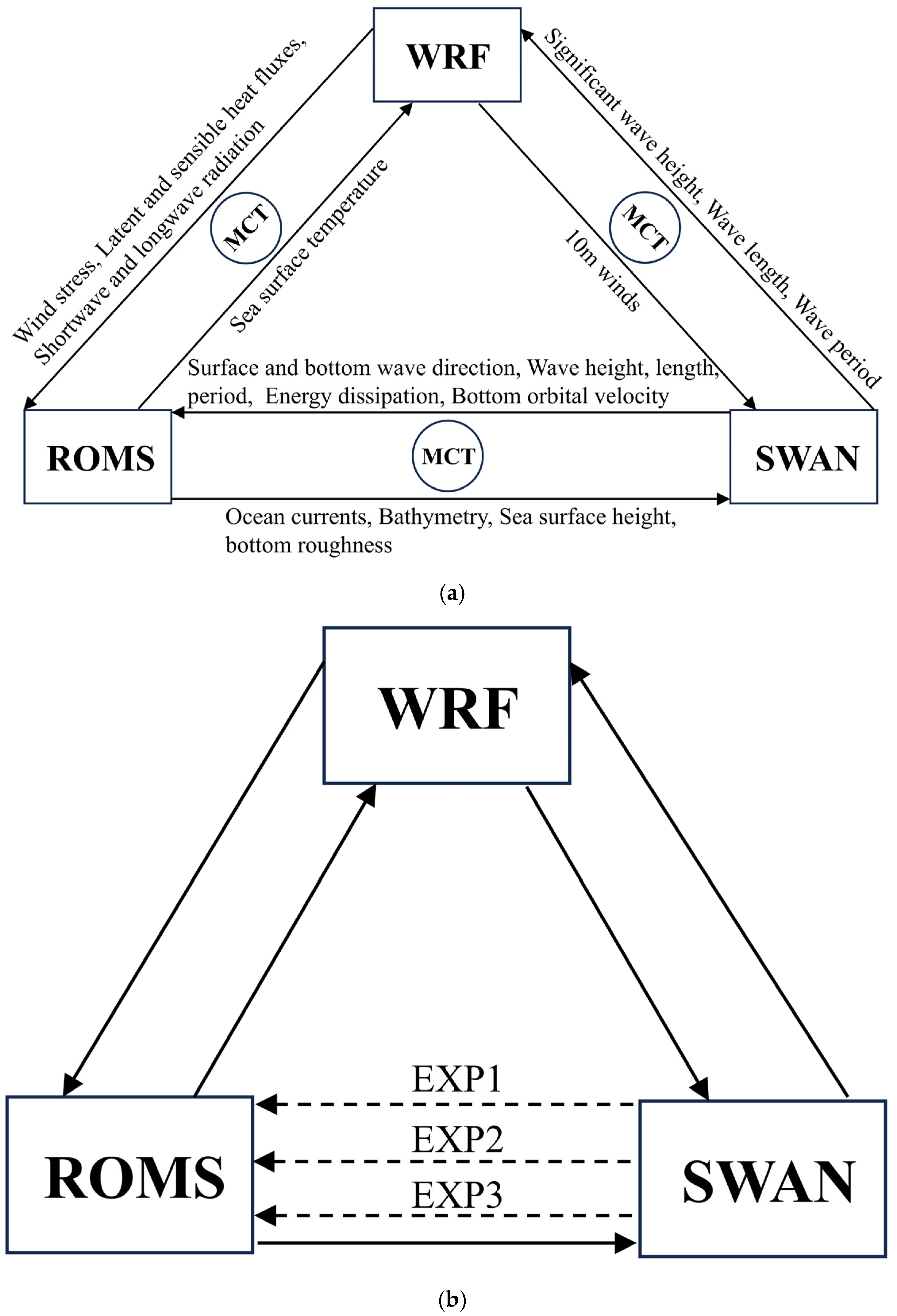
2.1. Experimental Programs

The coupling between the orbital velocity of surface waves and pre-existing turbulent fluctuations can generate additional turbulence, which modulates the vertical mixing of the ocean [21]. The vertical mixing induced by non-breaking waves is modeled using Reynolds stress formulation and Planck’s mixing length theory [21,38]:

$$Bv=\alpha {{\displaystyle \iint }}_{\overrightarrow{k}}{\displaystyle \frac{E(\overrightarrow{k})e^{2kz}\mathrm{d}\overrightarrow{k}\partial }{\partial z}}{({{\displaystyle \iint }}_{\overrightarrow{k}}{\omega }^{2}E(\overrightarrow{k})e^{2kz}\mathrm{d}\overrightarrow{k})}^{1/2}$$

(1)

where $E\left(k\right)$, $\omega$, $\overrightarrow{k}$, $z$ and are the directional spectrum of the wave, the angular frequency wave number, the unit vector in the wave direction and the depth from the sea surface, respectively. The constant factor $\alpha =1$ is taken.

In a previous study, Ru et al. [39] calculated the vertical eddy momentum coefficient and thermal mixing coefficient based on significant wave height, wavelength, wave period and other wave elements obtained from the WW3 wave model simulation using eigenwave parameterization theory. These coefficients were directly incorporated into the SBPOM circulation model to simulate global sea surface temperature, yielding favorable results. Similarly, Sun et al. [40] applied this wave mixing scheme, along with other wave effects, to a double typhoon case. The results demonstrated significant cooling near the typhoon, with greater cooling on the right side compared to the left. In this paper, we adopt the same method, incorporating this scheme into the COAWST model (EXP2) for comparison with the newly proposed scheme. Based on eigenwave parameterization theory, the wave-induced vertical eddy momentum and thermal mixing coefficients are denoted as $K_{wm}$ and $K_{wh}$. The expressions are:

$$K_{wm}={\displaystyle \frac{2a{k}^2\lambda }{\pi T}}{\mathrm{e}}^{{\displaystyle \frac{2\pi z}{\lambda }}}$$

(2)

$$K_{wh}={\displaystyle \frac{2P{k}^2}{g}}\delta {\beta }^3{W}^3{\mathrm{e}}^{{\displaystyle \frac{\mathrm{g}z}{{\beta }^2{W}^2}}}$$

(3)

where $k$ is the Karman constant, $a$ is the amplitude and is taken to be twice the Significant wave height, $T$ is the period of fluctuation, $W$ is wind speed, $\lambda$ is the wave length, $z$ is the depth from the sea surface to a certain position, $\beta$ is the wave age, $P$ is a dimensionless coefficient related to the Richardson number and $\delta$ and is the wave steepness. At the sea surface, it is generally taken as $k=0.4$, $\beta =1.0$, $P=0.1$, $\delta =0.1$, $\pi =3.14$, $g=9.8 \mathrm{m}\cdot {\mathrm{s}}^{-2}$. In general, the temperature is slower than the momentum mixing, so let $K_{wh}=P{K}_{wm}$ (has been widely used in marine modeling and performs well [39,40]). Significant wave height, wavelength, wave period and other wave elements obtained from the wave model simulation are used to calculate the vertical eddy momentum coefficients and thermal mixing coefficients, and the calculated $K_{wm}$ and $K_{wh}$ are directly added to the circulation model as part of the vertical eddy viscosity coefficient $K{\prime }_h$ and vertical diffusion coefficient $K{\prime }_m$.

$$K{\prime }_h=K_h+K_{wh}$$

(4)

$$K{\prime }_m=K_m+K_{wm}$$

(5)

where $K_h$ is the vertical diffusion coefficient of the temperature and salinity control equations in the ocean circulation model, and $K_m$ is the vertical viscosity coefficient of the momentum control equation. The definitions are:

$$K_h=ql{S}_h$$

(6)

$$K_m=ql{S}_m$$

(7)

where ${\displaystyle \frac{1}{2}}{q}^2$ and $l$ denote the turbulent kinetic energy and turbulent mixing length, respectively, and $S_h$ and $S_m$ are functions of the Richardson number $G_H$. It should be noted that when the boundary conditions $l=0$ are taken on the ocean surface, the corresponding $K_h=K_m=0$.

Although the aforementioned wave-induced mixing schemes have improved the issue of over-simulating the mixing layer, the results are still unsatisfactory, particularly during typhoons, where the wave-induced turbulence effect is severely underestimated. The interaction between the wave field and turbulence can transfer a significant amount of energy from the wave field to the turbulence. Therefore, if surface waves are present, the production of turbulent kinetic energy (TKE) in the upper ocean should include the influence of surface waves. In marine environments, non-breaking surface waves contribute energy to the turbulent dynamics rather than directly causing mixing [41]. In this scheme, the TKE dissipation rate due to wave-turbulence interactions caused by a typhoon is expressed as follows [42]:

$${\epsilon }_w=u_{*}^2{\displaystyle \frac{\partial \mathrm{u}}{\partial z}}$$

(8)

where $u_{*}$ is the friction velocity, $z$ is the distance below the mean sea surface, the horizontal velocity of the fluctuation is $\mathrm{u}=a\sigma {\mathrm{e}}^{{\displaystyle \frac{2\pi z}{\lambda }}}\cos {\displaystyle \frac{2\pi }{\lambda }}x\cos \sigma t$, $a$ is the amplitude, which is twice the significant wave height, the $T$ is the fluctuation period and the $\lambda$ is the wave length.

For a given defined location, the average rate of the water quality point over a cycle is [43]:

$$u={\displaystyle \frac{4a}{T}}{\int }_0^{{\displaystyle \frac{T}{4}}}u\mathrm{d}t={\displaystyle \frac{4a}{T}}{\mathrm{e}}^{{\displaystyle \frac{2\pi z}{\lambda }}}$$

(9)

It can be derived that:

$${\displaystyle \frac{\partial u}{\partial z}}={\displaystyle \frac{8\pi a}{\lambda T}}{\mathrm{e}}^{{\displaystyle \frac{2\pi z}{\lambda }}}$$

(10)

This scheme is similar to that described in [41], except it accounts for turbulence generated by non-breaking waves. As shown below, the turbulent kinetic energy dissipation rate decreases with depth:

$${\epsilon }_w={\displaystyle \frac{16\pi H_s{u}_{*}^2}{\lambda T}}{\mathrm{e}}^{{\displaystyle \frac{6\pi z^2}{\lambda }}}$$

(11)

where $H_s$ is the Significant wave height.

From an energy balance perspective, the energy transferred from non-breaking surface waves to turbulence should equal the rate at which wave-turbulence interactions generate turbulent kinetic energy (TKE) $P_w$, as expressed in the following equation:

$$P_w={\epsilon }_w$$

(12)

Therefore, it can be seamlessly incorporated into the shear generation term $P_s$ of the turbulence model (as shown in Equation (16) below) as an additional source of turbulence. The two components are then integrated to create a new shear generation term $P_{sw}$ within the turbulence model:

$$P_{sw}=P_s+P_w$$

(13)

Unlike the previously mentioned scheme, when incorporating additional turbulence, it is essential to concurrently modify the vertical kinematic viscosity, the diffusion coefficient and the turbulence generation term in the ocean model, as detailed below:

$$K{\prime }_h=K_h+K_w$$

(14)

$$K{\prime }_m=K_m+K_w$$

(15)

$$P_{sw}=P_s+P_w$$

(16)

where $K_w=a{u}_{s0}{e}^{3kz}$ [44], $u_{s0}$ is the magnitude of the Stokes drift velocity in the surface layer.

In this paper, the newly proposed scheme is incorporated into the COAWST model (EXP3), following the approach described above. It is then analyzed in comparison with both the original COAWST model scheme (EXP1) and the previously researched scheme (EXP2), the specific experimental steps are shown in Figure 1b.

2.2. Introduction and Setup of the Coupling Model

The Weather Research and Forecasting (WRF) model, developed by the National Center for Atmospheric Research (NCAR) and the National Centers for Environmental Prediction (NCEP), is widely used for typhoon-simulation studies [45]. The WRF model utilizes a structured grid and employs a time integration scheme based on either third-order or fourth-order Runge–Kutta methods. It incorporates an orthogonal curvilinear grid (Arakawa C) in the horizontal direction and topographic coordinates in the vertical direction. The model is based on the fully compressible non-hydrostatic Euler equations. The main grid of WRF spans from 103°E to 140°E and 10°N to 41°N, while the nested grids cover 105°E to 136°E and 12°N to 33°N, with resolutions of 30 km and 10 km, respectively, as illustrated in Figure 2.

The Simulating Waves Nearshore (SWAN) model, developed by Delft University of Technology, Netherlands, is a widely used numerical model for nearshore wave simulation [46]. SWAN simulates wave propagation, generation and dissipation in nearshore regions, addressing non-constant and non-linear wave effects such as wave breaking and whitecapping. Capable of calculating various wave parameters including wave height, direction and period, SWAN is suitable for multi-scale simulations from large-scale to local nearshore processes. Its grid range and resolution match the nested grid of WRF.

The Regional Ocean Modeling System (ROMS) is an ocean model based on a three-dimensional, non-linear, free-surface oblique pressure equation using Reynolds-averaged Navier-Stokes equations [47]. ROMS employs a finite-difference approximation on a horizontal Arakawa-C grid and vertical terrain-following coordinates with a non-isotropic stratification model. This setup enhances the simulation accuracy of the thermocline and bottom boundary layer by better modeling seafloor topography compared to traditional bathymetric layering. The grid extent and resolution of ROMS are consistent with the nested grid of WRF.

The Coupled Ocean–Atmosphere–Wave–Sediment Transport (COAWST) model is a comprehensive system for simulating and studying interactions among the atmosphere, waves and ocean [48]. As shown in Figure 1a, COAWST integrates several independent sub-models: WRF for atmospheric processes, SWAN for wave simulation and ROMS for ocean dynamics. These sub-models are coupled via the Model Coupling Toolkit (MCT), allowing simultaneous simulation of multiple interacting natural processes for more accurate environmental predictions. During initialization, MCT records the zonation of atmospheric, oceanic and wave model simulations and sets up variable transfer directions among the components. Throughout the model run, components are integrated independently, with variables exchanged at specified coupling intervals. In the latest COAWST version, the atmospheric component provides a 10 m horizontal wind field to the waves and supplies ocean heat and momentum fluxes through the atmospheric boundary layer scheme. The ocean model offers SST to the atmosphere and provides sea surface current (SFC), free height (FH) and ocean topography (OT) to the waves. The wave component calculates significant wave height (SWH), wavelength and directional angle (DA) and returns these parameters to the ocean model. Additionally, it supplies the atmosphere with a dynamic roughness parameter, replacing the original constant coefficient scheme of the atmospheric boundary layer (ABL). The parameterization schemes for the various modes are detailed in

Table 1. Summary of the configurations of the three component models.

	WRF	SWAN	ROMS
Domain	DO1: 140 × 116 (30 km)	DO1: 591 × 438 (10 km)	DO1: 590 × 437 (10 km)
	DO2: 591 × 438 (10 km)
	50 eta levels		40 sigma levels
Dynamics	DO1: dt = 48 s, DO2: dt = 16 s	dt = 60 s	dt = 60 s
Physics	Mp_physcis: WSM 6-class graupel	Whitecapping physics: KOMEN	Momentum equation physics: TS_U3HADVECTION
	Ra_lw_physics: RRTMG	Whitecap crushed Physics: Hasselman	Vertical mixing physics: MY2.5 mixing
	Ra_sw_physics: RRTMG	Bottom Friction Physics: Collins	Tidal physics: UV_TIDES
	Sf_sfclay_physics: Monin-Obukhov
	Sf_surface_physics: Noah
	Bl_pbl_physics: TS_U
	Cu_physics:Kain-Fritsch

.

2.3. Study Area and Datasets

Considering the typhoon’s track, intensity, scope of impact and damage, the 2021 super typhoon In-Fa was chosen as the subject of this study. It was the longest-lasting typhoon to affect China’s mainland since records began, causing extensive storm impacts and substantial cumulative rainfall. Typhoon In-Fa, the sixth typhoon of 2021, formed at 02:00 UTC on 18 July in the northwest Pacific Ocean. It strengthened to a strong tropical storm by the morning of 19 July, reached typhoon strength on July 20 and became a strong typhoon by the morning of 21 July. It made landfall in Putuo, Zhoushan, Zhejiang Province, at approximately 12:30 UTC on 25 July, with a maximum wind speed of 38 m/s (Level 13, typhoon level). The interaction of In-Fa with Typhoons No. 7 Cempaka and No. 8 Nepartak, along with the northeastward shift of the subtropical high pressure, resulted in weak steering flows and a complex trajectory for “In-Fa” (Figure 3a), and the path of the typhoon was obtained from the best track data supplied by the Japan Meteorological Agency (JMA).To quantify the impact of wave mixing on SST cooling, we performed two sensitivity experiments: one with and one without wave mixing effects. We used four main statistical parameters—peak error (PE), mean absolute error (MAE), root mean square error (RMSE) and correlation coefficient (COR)—to assess the model’s simulation accuracy. These parameters are calculated as follows:

$$PE=(y_{max}-x_{max})$$

(17)

$$MAE={\displaystyle \frac{1}{N}}\sum _{i=1}^N|(y_i-x_i)|$$

(18)

$$RMSE=\sqrt{{\displaystyle \frac{1}{N}}\sum _{i=1}^N{\left(y_i-x_i\right)}^2}$$

(19)

$$COR={\displaystyle \frac{{\displaystyle \sum _{i=1}^N(x_i}-\overline{x})(y_i-\overline{y})}{\sqrt{{\displaystyle \sum _{i=1}^N(x_i}-\overline{x}{)}^2{(y_i-\overline{y})}^2}}}$$

(20)

where $x_i$ and $y_i$ represent the observed and simulated values, respectively. $\overline{x}$ and $\overline{y}$ represent the mean of the observed and simulated values, respectively. $N$ represents the number of data points.

The topographic data used in the model are from the ETOPO1 dataset provided by the NOAA National Centers, with a resolution of 1′ × 1′ (Figure 2). Wind field data are sourced from the Global Forecast System (GFS), developed and maintained by the National Centers for Environmental Prediction (NCEP), with a horizontal resolution of 0.25° and updated every 6 h. Daily mean heat flux data, including shortwave radiation, longwave radiation, sensible heat flux and latent heat flux, are obtained from the European Centre for Medium-Range Weather Forecasts (ECMWF) at a resolution of 0.25°, with updates every hour. Initial temperature and salinity fields, along with lateral boundary conditions, are derived from the Hybrid Coordinate Ocean Model (HYCOM) with a resolution of 0.08° × 0.08°.

To verify the accuracy of the wind and wave simulations, data from the Jason-3 satellite altimeter in the Ku-band were used. We selected data from four satellite altimeter scans during the typhoon for wave validation, as shown in Figure 3c. The lines from left to right represent the satellite altimeter trajectories on 19 July, 20 July, 23 July and 24 July, respectively.

Argo buoy data were collected by the Global Argo Program (Array for Real-time Geostrophic Oceanography), which has been operational since 2000. Thousands of autonomous Argo buoys, capable of diving to 2000 m depth and resurfacing, collect data on ocean temperature, salinity and depth. The locations of the Argo buoys used in this study are shown in Figure 3b.

The Global Drifter Program (GDP), managed by the U.S. National Oceanic and Atmospheric Administration (NOAA), deploys thousands of drifter buoys worldwide to collect high-quality oceanographic data. These data are utilized in scientific research, weather forecasting, ocean management and environmental protection. The locations of the drifter buoys selected for this study are shown in Figure 3d.

The initial field, the driving field and the validation data for running this case are all open data, as shown in

Table 2. Data and sources.

Data	Data Sources
Topographic data	ETOPO1 (http://www.ngdc.noaa.gov/mgg/global/, accessed on 3 March 2024)
Wind data	GFS (https:/nomads.ncep.noaa.gov/, accessed on 3 March 2024)
Heat flux data	ERA5 (https://www.ecmwf.int/, accessed on 3 March 2024)
Initial field data	HYCOM (https://www.hycom.org/, accessed on 3 March 2024)
Validation data	JASON-3 (https://www.aviso.altimetry.fr/en/home.html, accessed on 3 March 2024)
	OISST (https://www.hycom.org/, accessed on 3 March 2024)
	Argo (http://www.argo.org.cn/, accessed on 3 March 2024) Drifter (https://www.aoml.noaa.gov/global-drifter-program/, accessed on 3 March 2024)

.

3. Results

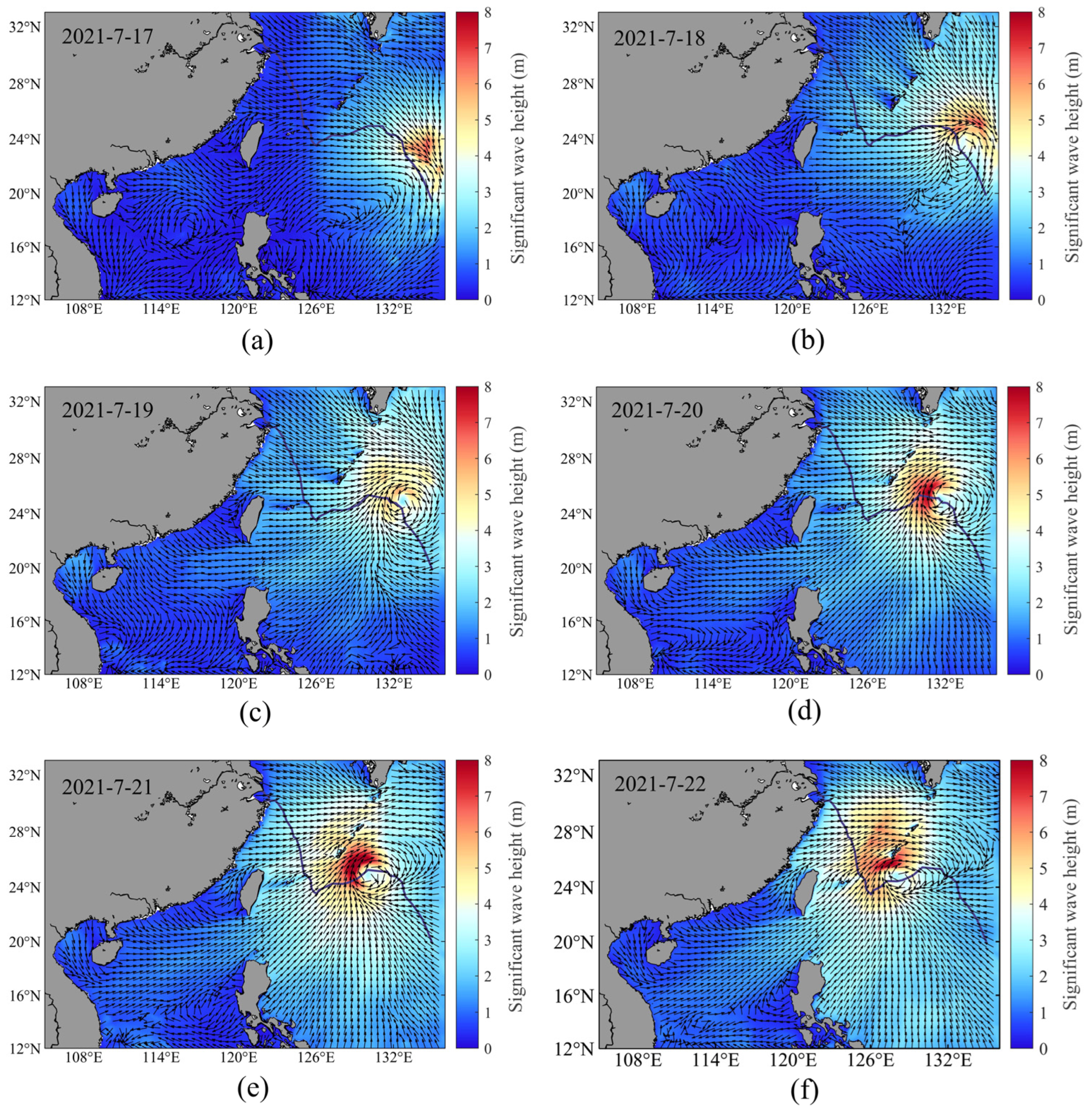
3.1. Wave-Simulation Results

During a typhoon, the intense wind field generates large waves at the sea surface. Figure 4 illustrates the characteristics of significant wave height (SWH) and wave direction distributions simulated by the COAWST coupled model from the onset of Typhoon In-Fa to its landfall. In the figures, black arrows indicate wave directions, and colors represent significant wave heights. The typhoon’s strong waves significantly impact oceanic conditions. Overall, SWH in non-typhoon regions remains below 1.5 m, whereas in the typhoon-affected area, it can reach up to 8 m, with a maximum observed height of 13.3 m. On 17 July, when the typhoon first formed as a tropical depression, the generated waves had not yet reached the South China Sea. Significant wave heights began to rise notably on 20 July, affecting the South China Sea waters. By 21 July, SWH in the vicinity of the typhoon peaked, coinciding with the typhoon’s maximum intensity as a super typhoon. The numerical results reveal that the wave responses on either side of the typhoon’s path differ: the intensity of wave response on the right side consistently exceeds that on the left. This observation aligns with previous findings [49]. The accurate simulation of the wave field during Typhoon In-Fa offers valuable data for studying wave-induced upper-ocean mixing.

To verify the accuracy and reliability of the simulation results, we conducted a multi-perspective comparison of significant wave heights (SWH) during the typhoon using data from the Jason-3 satellite. The SWH outputs from the SWAN model were extracted and analyzed along the satellite altimeter’s path, as illustrated in Figure 5. Despite some deviations in the simulation results, the significant wave heights generally exhibit good agreement with the observed values, demonstrating that the numerical simulation accurately represents the SWH. This consistency indicates that the simulation effectively captures the spatial distribution of the wave field.

Table 3. Comparison of simulated values and satellite data.

Track	Satellite Peak (m)	Simulated Peak (m)	PE (m)	MAE (m)	RMSE (m)	COR
C1	5.152	4.767	0.385	0.342	0.366	0.871
C2	6.463	6.146	0.317	0.392	0.389	0.836
C3	4.177	3.918	0.259	0.296	0.314	0.943
C4	6.291	6.025	0.266	0.287	0.294	0.951

displays the PE, MAE, RMSE and COR values for both simulated and measured data. The results show that the COAWST simulation closely matches the Jason-3 satellite data, with simulated values slightly lower than the observed values. The RMSE values range from 0.29 to 0.39 m. All COR values exceed 0.8, indicating a strong correlation between the simulated and measured SWH values.

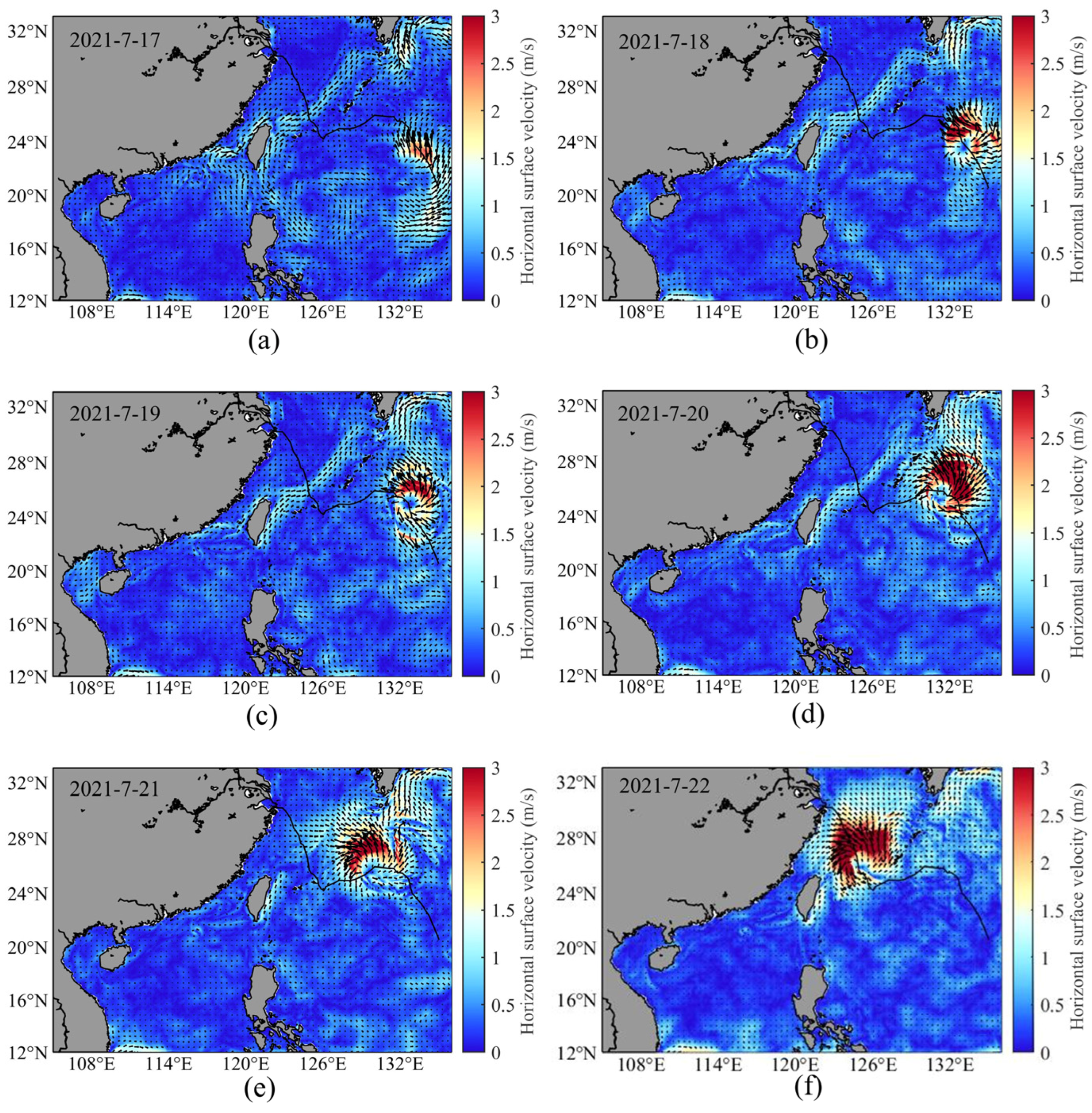
3.2. Simulated Currents

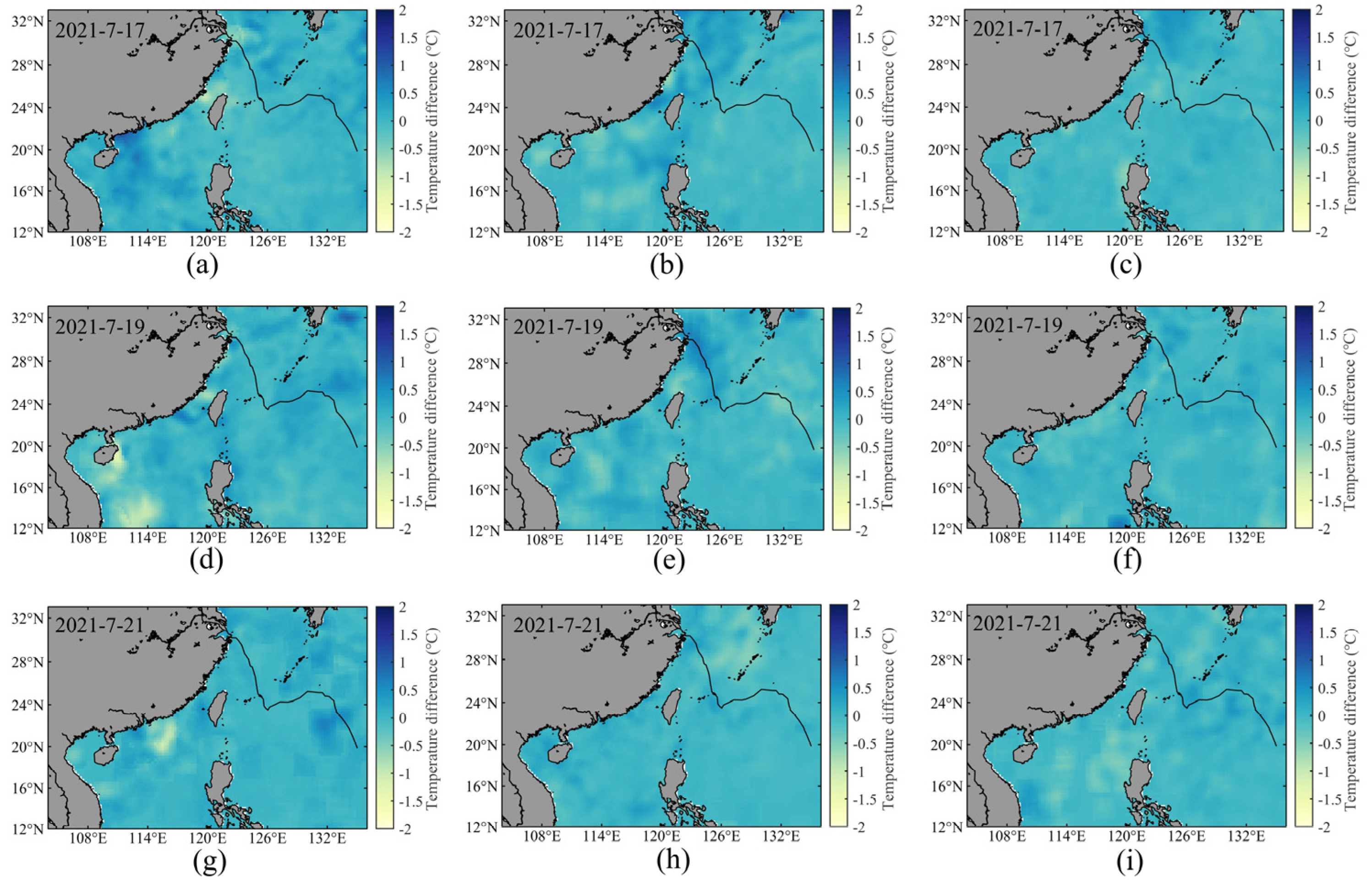
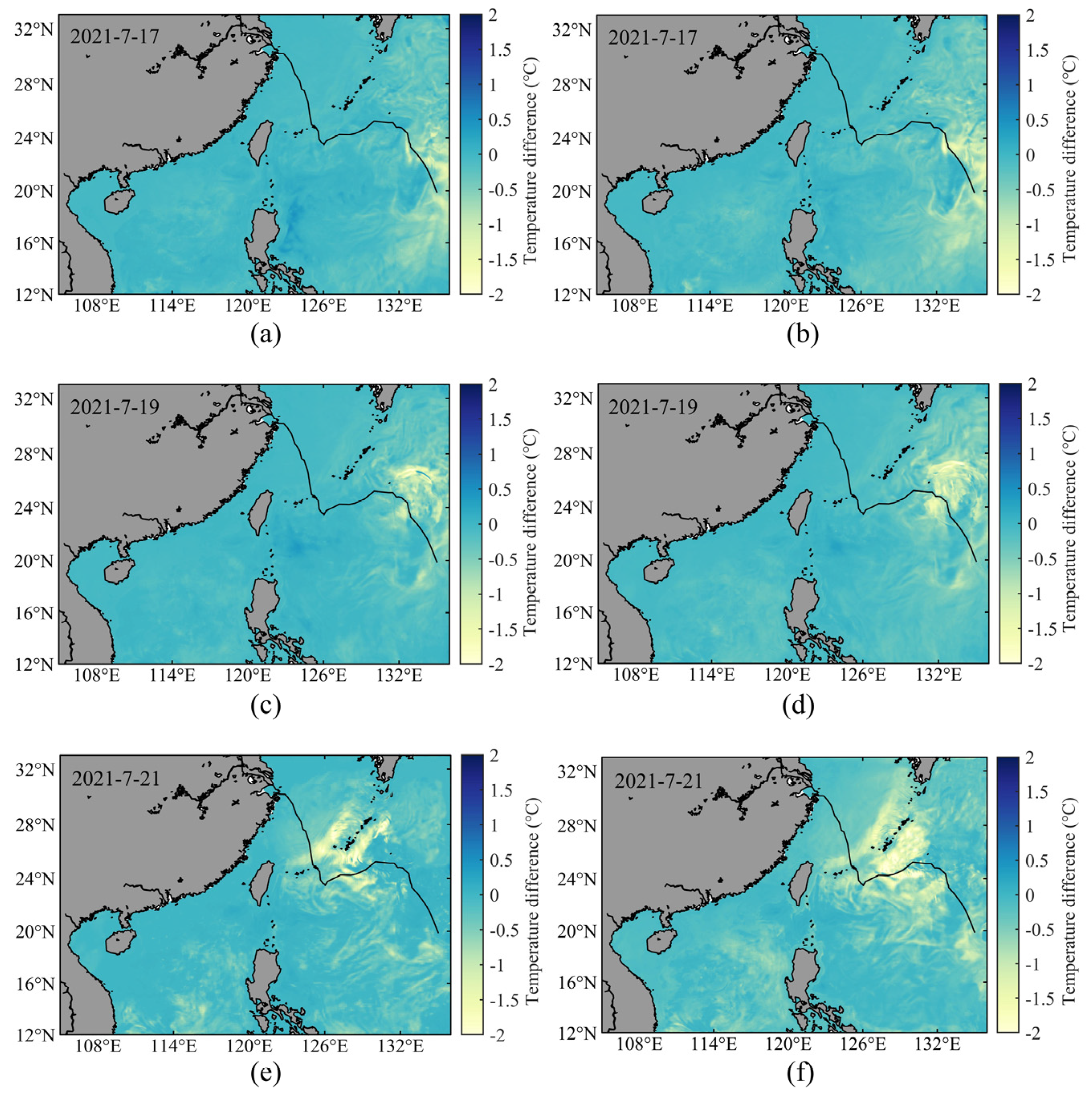
During the impact of Typhoon In-fa, the strong cyclonic wind field caused significant disturbances in the upper layer of the East China Sea. Figure 6 shows the scalar distribution of the surface current field in the South China Sea during In-Fa The current velocity U in the South China Sea during the typhoon is relatively uniform, with an average velocity of less than 0.5 m/s. Seasonal fluctuations in the seawater density field, particularly at the surface, contribute to these changes. During the typhoon, the velocity of the ocean currents around the typhoon’s path significantly increased, showing a close correlation with the typhoon’s intensity. On 22 July, the maximum mean current velocity exceeded 5 m/s, with the velocity on the right side of the typhoon path being significantly higher than on the left.

3.3. Simulated SST

Due to the high quality and wide use of OISST data, which can provide a reliable reference in both calm and extreme weather, and we are able to effectively validate the accuracy of the model under extreme conditions based on the existing research methods, we simulated the SST from this model with the same resolution as interpolated into the OISST data and subtracted it from the OISST data, and the results are shown in Figure 7. The results indicate that the simulated SST is slightly higher than the actual values in most sea areas, with temperature differences within 1 °C, demonstrating the effectiveness of this ocean simulation. Comparing the three sets of experiments, it can be seen that the difference between the simulated SST and OISST is significantly reduced by adding the wave mixing effect, which indicates that the addition of the wave mixing effect is necessary to improve the accuracy of the model prediction in numerical simulations in this sea area.

To directly reflect the effect of droop mixing on the SST simulation, we calculated the difference between the simulated SST values considering droop mixing and those without considering droop mixing, to obtain the improvement in the simulated values $\alpha$:

$$\alpha ={SST}_{aw}-{SST}_{uw}$$

(21)

where ${SST}_{aw}$ is the simulation result of sea surface temperature with the addition of wave-induced mixing and ${SST}_{uw}$ is the simulation result of sea surface temperature without the addition of wave-induced mixing.

The distribution of the simulated value improvements $\alpha$ is shown in Figure 8. The vertical mixing primarily has a cooling effect on the SST simulation, and the cooling path of the SST changes with the movement of the typhoon, which is especially noticeable near the typhoon’s path. In the early stages of the typhoon, the intensity of both the wind and wave fields is low, resulting in slight cooling of the SST due to wave-induced vertical mixing. As the typhoon intensifies, the effect of vertical mixing on SST cooling in the typhoon-affected area becomes more pronounced and widespread. By 21 July, when the cooling effect is at its peak, the cooling in the sea area near the typhoon’s path averages 1.6 °C. The response of the typhoon to the ocean is a typical process of sea–air–wave interaction. When the typhoon passes, the cyclonic wind stress causes Ekman pumping, which lifts the thermocline and cools the sea surface, known as the “cold pumping” effect [50,51]. Additionally, the strong winds from typhoons generate large waves that convert kinetic energy into turbulent energy when breaking, enhancing turbulent mixing in the ocean’s surface layer. Wave breaking intensifies the vertical exchange between the surface and lower layers, with cold water upwelling and warm water sinking, increasing the energy and matter exchange and causing a significant decrease in SST [52]. The greater cooling on the right side of the typhoon’s forward direction in the Northern Hemisphere is due to two reasons: first, before the typhoon passes, the area experiences southeasterly flow, and as the typhoon moves away, the wind direction changes clockwise, enhancing wind-induced inertial flow and shear-induced vertical mixing [53,54]; second, the typhoon’s movement speed, combined with the cyclonic wind field, leads to stronger winds on the right side [55], resulting in greater seawater cooling. Additionally, the experimental results show that the cooling effect of EXP3 is stronger than that of EXP2, with more significant differences in typhoon intensity cooling. This is mainly due to the more substantial turbulent mixing effect in EXP3, which further enhances vertical exchange and momentum transfer in the surface layer, leading to a larger cooling amplitude.

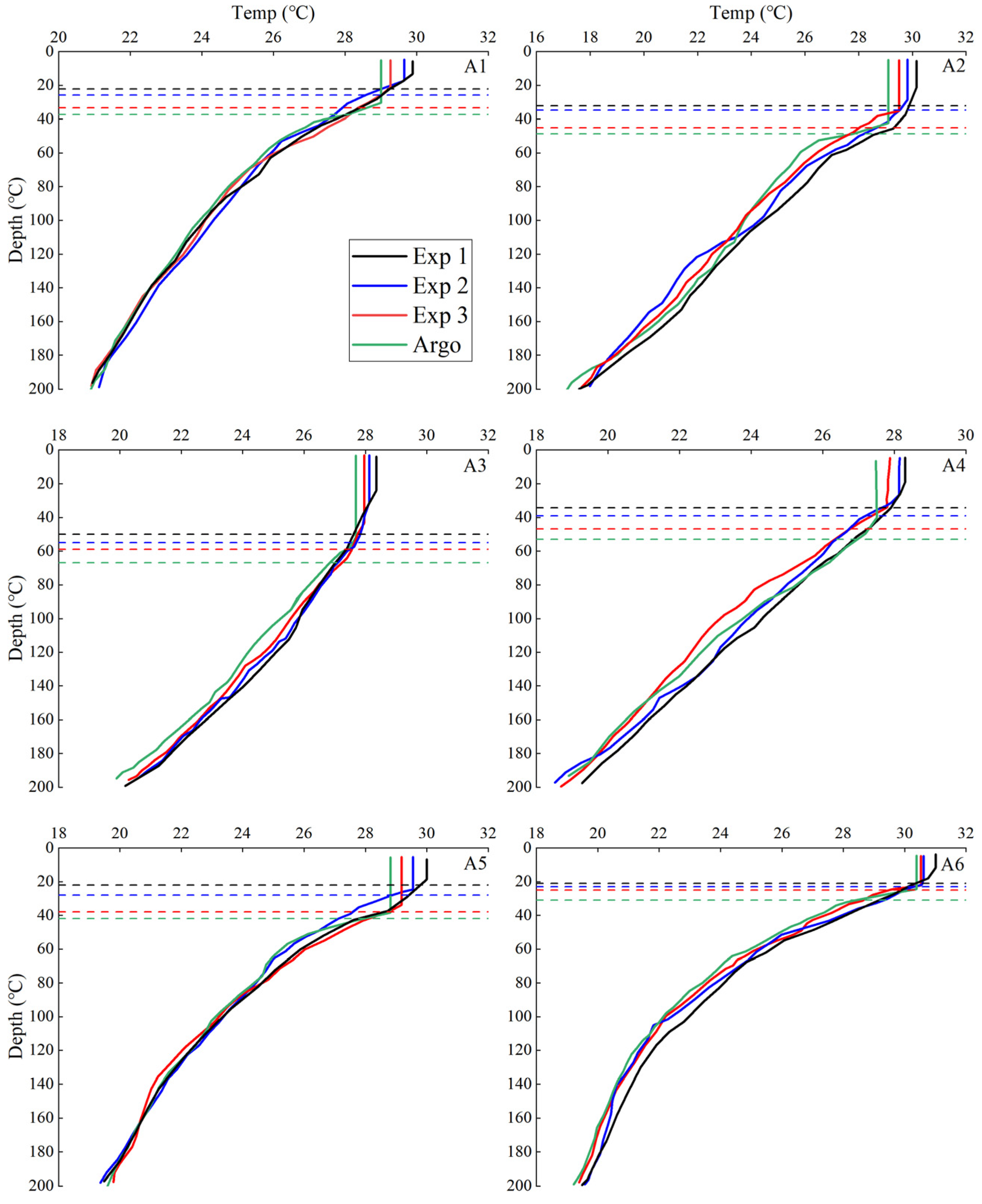
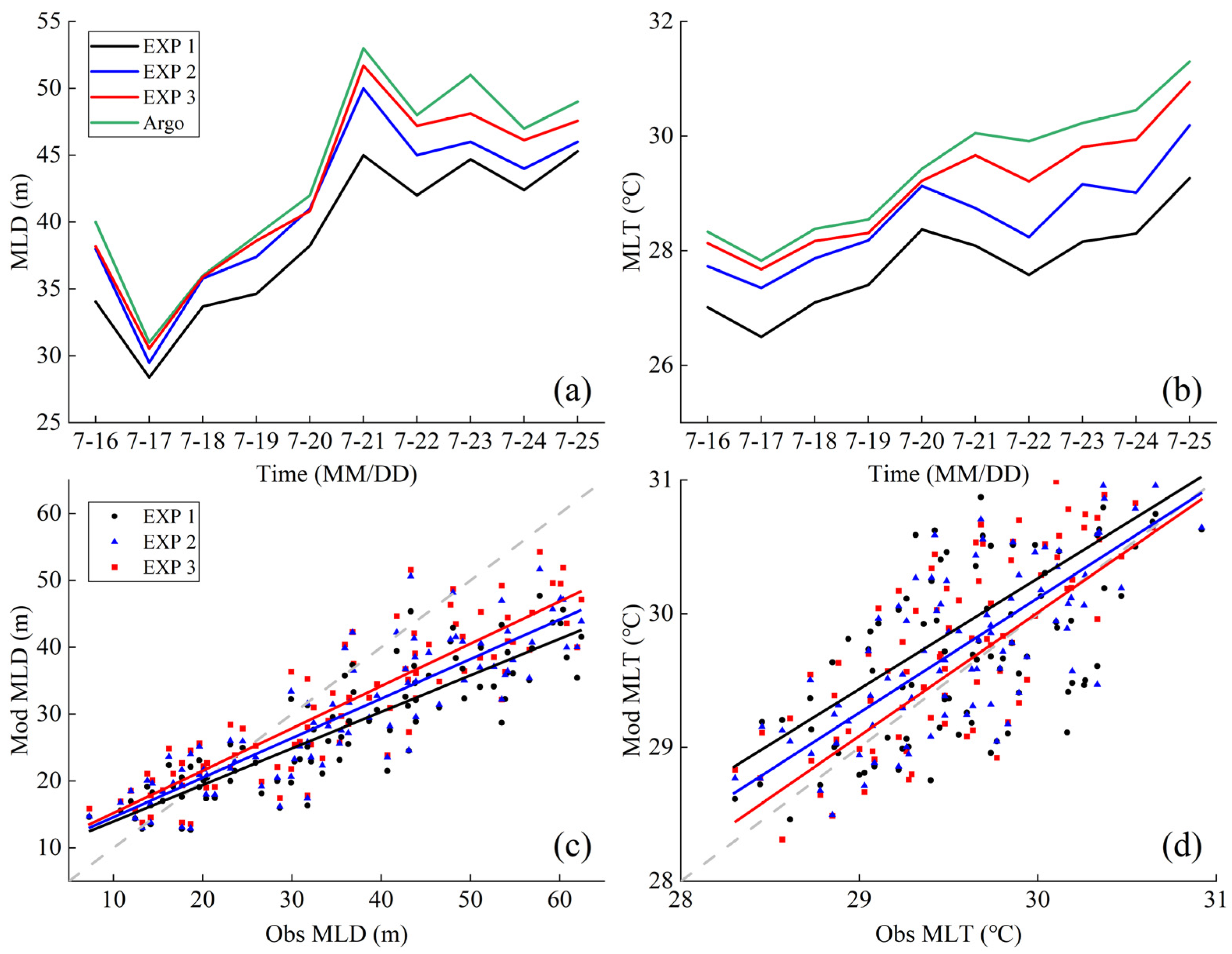
3.4. The Simulated Results of Mixed-Layer Temperature

Six buoys were selected to compare the temperature profiles: without considering vertical mixing and with considering vertical mixing, as shown in Figure 9. After analyzing the temperature profiles, it was found that the simulated temperature profiles, after considering vertical mixing, closely resemble the measured temperature profiles of the buoys. This indicates that the simulated values more accurately determine the upper boundary of the thermocline after accounting for the vertical mixing effect, thereby improving the analysis of thermocline characteristics. Additionally, wave-induced vertical mixing not only reduces SST but also affects the vertical seawater temperature. The vertical mixing effect penetrates the depth of its influence, impacting the entire mixing layer [56]. Upwelling compensates for surface water, enhancing convection in the mixing layer, and this enhanced convection between upper and lower seawater further reduces SST. By comparing the three sets of experiments, the results show that the simulated temperature profiles of EXP3 are closer to the actual measurements of the Argo floats than those of EXP2, suggesting that the temperature profile of EXP3, through enhanced turbulent mixing, more accurately matches the actual measurements. This indicates that EXP3 can more precisely simulate the ocean’s response during typhoons by enhancing turbulent mixing.

The vertical mixing effect deepens the vertical mixing coefficient and can expand it to three times its original value in certain areas. Wave mixing plays a significant role in the formation of the thermocline, and it has been shown that numerical model simulation issues and the shallow depth of the mixing layer can be addressed by superimposing the vertical mixing coefficient with different forms of wave mixing effects [57]. Figure 10 shows the variation of vertical mixing profiles at six selected Argo buoys during the passage of Typhoon In-Fa. Kh represents the vertical thermal mixing coefficient, and Km represents the vertical eddy momentum. The red line represents the mixing result after including the wave-induced vertical mixing effect, while the black line represents the mixing result without the wave-induced vertical mixing effect.

Figure 10 illustrates that mixing increases significantly during the passage of a typhoon when considering the vertical mixing effect. The mixing intensity is greater near the typhoon than farther away from it. The coefficients of the vertical mixing depths from the six buoys are limited to 80 m. At buoy A3, which is farther from the typhoon, the Km and Kh are smaller than those near the typhoon. However, after adding the vertical mixing effect, the Km and Kh increase significantly, showing that wave-induced mixing is notably strengthened. At buoy A5, also farther from the typhoon, the mixing degree does not deepen without adding the vertical mixing effect to the model. However, after adding the wave effect, the mixing coefficients increase significantly, although the vertical mixing depth is limited to 60 m. This may be because during the passage of Typhoon In-Fa, buoy A5 in the South China Sea was far from the typhoon’s center. The waves generated by the typhoon traveled a path with more islands, dissipating most of the energy. The vertical mixing depth is thus deepened, and the mixing effect may control the formation of the thermocline to some extent, resulting in more homogeneous mixing of the upper ocean.

The response of the upper ocean to the typhoon is manifested in the changes in the ocean’s mixed layer depth (MLD) and mixed layer temperature (MLT). In this study, we define the MLD as the depth where the temperature is 0.5 °C lower than the surface temperature, and the MLT as the average temperature within the MLD. To better represent this structure and its variability, as well as the role of waves, we use Argo buoy data (Figure 3b) and compare it with simulations from three experiments. The Array for Real-time Geostrophic Oceanography (ARGO) floats can measure temperature and salinity in the global ocean (0–2000 m), even during typhoons. Therefore, ARGO data provide a good response to the structure of the upper ocean and its changes after being affected by a typhoon [58].

Figure 11 shows the MLD and MLT time series plots of the Argo observation data with the three experiments. The observed data show that the depth of the mixed layer at the Argo buoy deepened rapidly from a minimum of 31 m to a maximum depth of 53 m due to the typhoon (Figure 11a). The MLDs of all three experiments show a similar trend to the observations, but the MLD simulated by EXP1 shows too small a change, deepening from 28 m to a maximum depth of 45 m, which is quite different from the observations. The MLD simulated by EXP2 reaches a maximum mixed layer depth of 48 m, an increase of 3 m compared to the experiment without vertical mixing (EXP1), highlighting the importance of wave-induced mixing effects. Further comparison between the results of experiments EXP2 and EXP3 reveals that the trend of the mixed layer simulated by EXP3 is much closer to the observation, and EXP3 shows stronger superiority during the period of higher typhoon intensity (21 July to 24 July).

Figure 11b shows the changes in MLT after the typhoon impact. In the pre-typhoon period, the trend of MLT is similar to that of MLD. The simulated MLT is significantly improved by considering the wave-induced mixing effect, with the maximum decrease in EXP2 compared to EXP1 being 0.6 °C, while the maximum decrease in EXP3 compared to EXP1 reaches 2 °C.

To further investigate the effect of vertical mixing on the upper ocean during the typhoon, we compared the MLD and MLT data from all observations during the typhoon with the results of the two experiments (Figure 11c,d). In this study, the COAWST model, which incorporates the wave-induced mixing effect, significantly affects the sea surface current velocity and sea surface temperature. As shown in

Table 4. Comparison of simulated MLD and MLT with buoy data.

	EXP1				EXP2				EXP3
	PE (m)	MAE (m)	RMSE (m)	COR	PE (m)	MAE (m)	RMSE (m)	COR	PE (m)	MAE (m)	RMSE (m)	COR
MLD (m)	26.54	8.85	11.05	0.84	21.94	6.58	8.55	0.88	18.54	5.25	6.13	0.92
MLT (°C)	1.55	0.55	0.65	0.52	1.14	0.46	0.53	0.74	1.02	0.41	0.46	0.64

, By comparing the different experimental conditions, it is found that EXP3 exhibits obvious advantages. The MLD metrics in EXP3 show that the PE decreases from 26.54 in EXP1 to 18.54, the MAE decreases from 8.85 to 5.25 and the RMSE decreases from 11.05 to 6.13, while the correlation coefficient (COR) improves from 0.84 to 0.92, indicating a significant reduction in error and an improvement in prediction accuracy. For MLT, the PE of EXP3 decreases to 1.02, and the MAE and RMSE are reduced to 0.41 and 0.46, respectively. Although the correlation fluctuates slightly, the reduction in overall error further proves the significant improvement of EXP3 in model prediction. These results suggest that EXP3 significantly improves the model’s ability to predict sea surface current speed and temperature by enhancing turbulent mixing and momentum transfer in the near-surface layer.

Figure 12 illustrates the changes in ocean temperature before and after the typhoon’s transit under three sets of experiments. We selected two points, B1 and B2, in Figure 3b for the study; B1 is located on the left side of the typhoon path, and B2 is located on the right side of the typhoon path and both of them are at the same distance from the center of the typhoon. The vertical coordinates of the figure indicate the ocean depth, the horizontal coordinates indicate the time and the contour lines show the temperature differences.

For the left side of the typhoon (Figure 12c,e), the temperature difference between the shallow and deep waters before the transit is small, indicating that the wave-induced mixing effect does not have much effect on the seawater temperature. During the typhoon’s transit, the temperature difference in the shallow water column (e.g., 0–50 m) began to increase, indicating that cold water rises from the deeper layers resulting in cooling of the shallow layers, but the temperature of the deeper water column did not change much. After the passage of the typhoon, the temperature difference in the shallow water column gradually decreased, the temperature began to recover, the influence of wave-induced mixing effect weakened and the temperature change in the deep water column remained small. In contrast, on the right side of the typhoon (Figure 12d,f), the temperature difference between the shallow and deep water bodies before the transit was also smaller. During the typhoon’s transit, the temperature difference in the shallow water column increased significantly, indicating significant cooling due to wave-induced mixing effects, and the temperature difference in the deeper water column also began to increase, showing that the rise of deeper, colder water affected the deeper water column. After the crossing, the temperature difference in the shallow water body gradually decreased, but the recovery was slower than that on the left side, indicating that the wave mixing effect on the right side of the typhoon was stronger and lasted longer than that on the left side, and that the temperature difference in the deeper water body was also gradually decreasing but recovering more slowly.

Comparing the results of the three sets of experiments (Figure 12c–f), it can be seen that the effect of EXP3 on the upper-ocean temperatures is larger than that of EXP2 and EXP1 in both the left and right sides of the typhoon, because the strong winds brought by the typhoon and the new wave-induced mixing parameterization scheme significantly enhance turbulent mixing in the surface layer in EXP3, which leads to a more efficient transfer of momentum and heat from the lower to the surface layer, and a more homogenization of the upper-ocean temperature, thus increasing the mixing temperature. more homogenized, thus increasing the depth of the mixed layer.

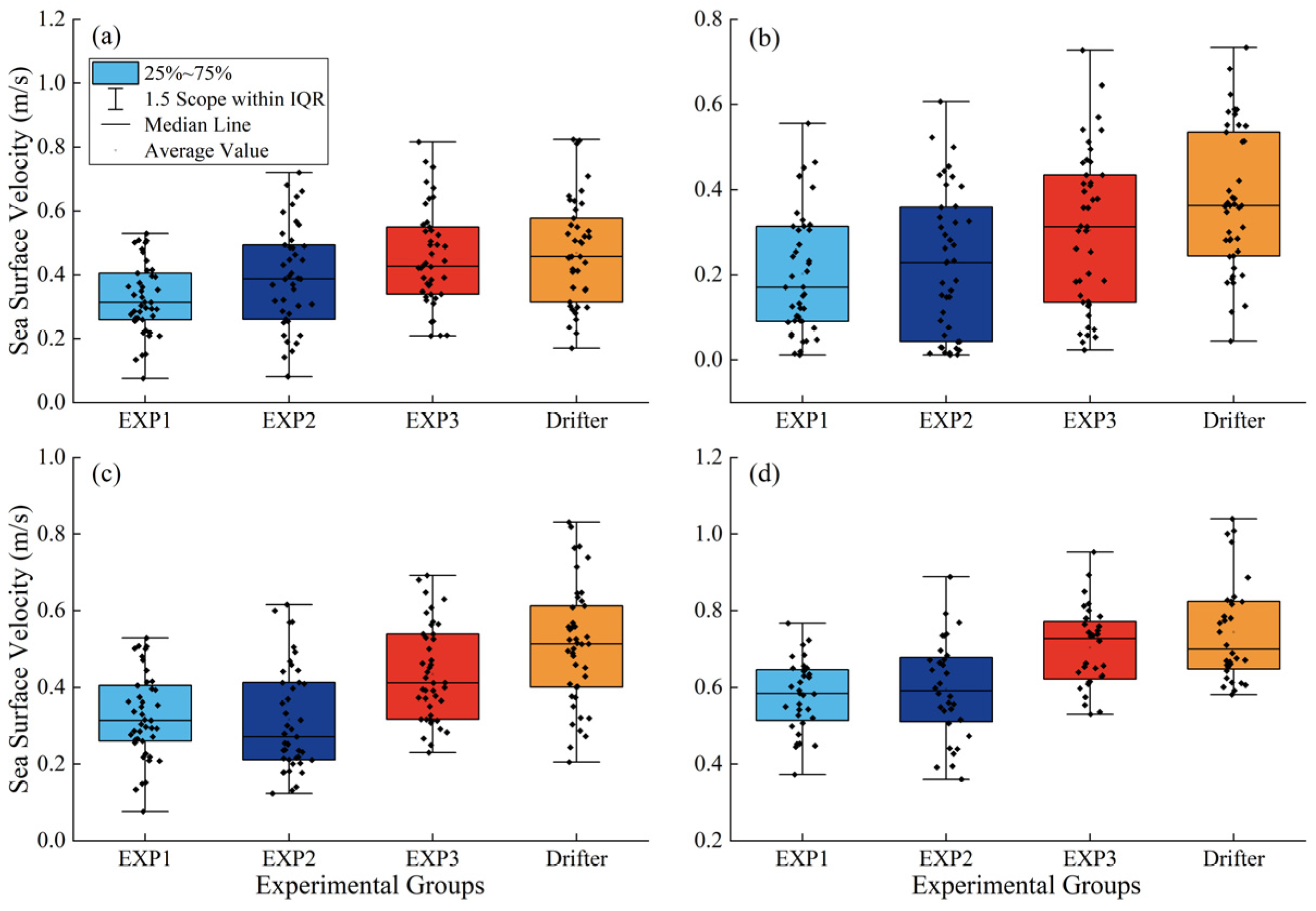
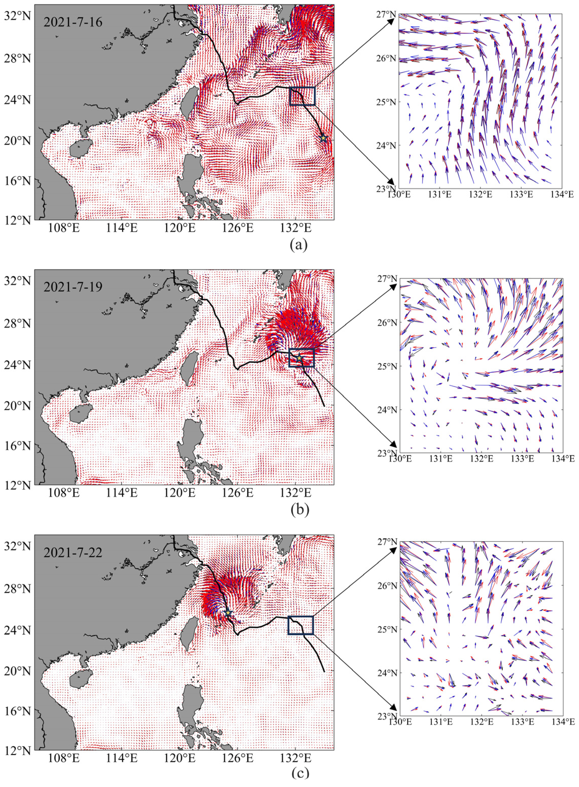
3.5. Effect on Surface Current Field

The dynamics during a typhoon are complex. Previous studies have demonstrated that the wave-induced mixing effect (one of the wave-induced stress terms) alters the distribution of surface currents, which in turn affects the energy conservation equation and subsequently influences SST [59]. Figure 13 compares the outputs of the three experiments with the measurements from selected drifter buoys. The results indicate that SST values from EXP3 are higher than those from EXP1 and EXP2 and are closer to the measured values from the drifter buoys. Overall, incorporating the wave mixing effect into the COAWST model results in increased sea surface current velocities and decreased SST. This is because the wave mixing effect enhances turbulent mixing and momentum transfer in the near-surface layer. Wave breaking injects momentum into the ocean’s surface layer, increasing surface turbulence and causing momentum to be transported from the lower water column to the upper layer, thereby increasing sea surface current velocity. Simultaneously, this enhanced turbulent mixing causes cold water to rise from deeper layers and heat to diffuse downward, resulting in a decrease in sea surface temperature.

Figure 14 illustrates the distribution of the sea surface current field during the passage of the typhoon. On 19 July, when the typhoon passed through the enlarged region on the right, the current flow direction changed. Most of the area exhibited a clear deviation to the right, while very few areas showed a deviation to the left of the typhoon’s path. The side closer to the typhoon showed a more pronounced rightward deviation, with the current deflection during the typhoon crossing being greater than before and after the crossing. Conversely, on the side farther from the typhoon, the direction shift was less pronounced. This phenomenon is primarily due to the Coriolis force, which causes inertia in moving objects due to the Earth’s rotation. In the oceans, the Coriolis force deflects currents to the right in the Northern Hemisphere and the left in the Southern Hemisphere [54,60]. While vertical mixing tends to stabilize the surface flow, this stable flow is more influenced by the Coriolis force, causing a greater deflection to the right. A comparison of EXP2 and EXP3 reveals that the flow deflection in EXP3 is generally more significant than in EXP2. This is attributed to the stronger turbulent mixing effect in EXP3, which enhances turbulence intensity and momentum transfer in the near-surface layer. Stronger turbulent mixing results in more effective vertical momentum exchange, making the surface layer flow more stable and thereby more susceptible to the Coriolis force, leading to greater flow deflections. In contrast, the weaker turbulence intensity and insufficient vertical mixing in EXP2 result in a less stable surface flow and less significant flow deflection compared to EXP3.

4. Conclusions

Wave interactions are crucial for energy exchange between the atmosphere and ocean. This paper presents a fully coupled sea–wave–air model based on the COAWST framework, applied during Typhoon 2106 In-Fa, and compares the results to observational data. The model accurately reproduces hydrodynamic processes under both calm and typhoon conditions. The East China Sea and South China Sea, connecting the Western Pacific and Indian Oceans, are vital for global climate patterns due to their unique geographic position and significant maritime ecosystems. Studying these regions refines global climate predictions and ocean circulation models. The proposed wave-induced mixing scheme, while demonstrated in these areas, is also applicable to other tropical cyclone-prone regions like the Atlantic and Indian Oceans. Extending this scheme to global climate models could further validate its effectiveness and impact on the global ocean system. The main conclusions are as follows:

(1)

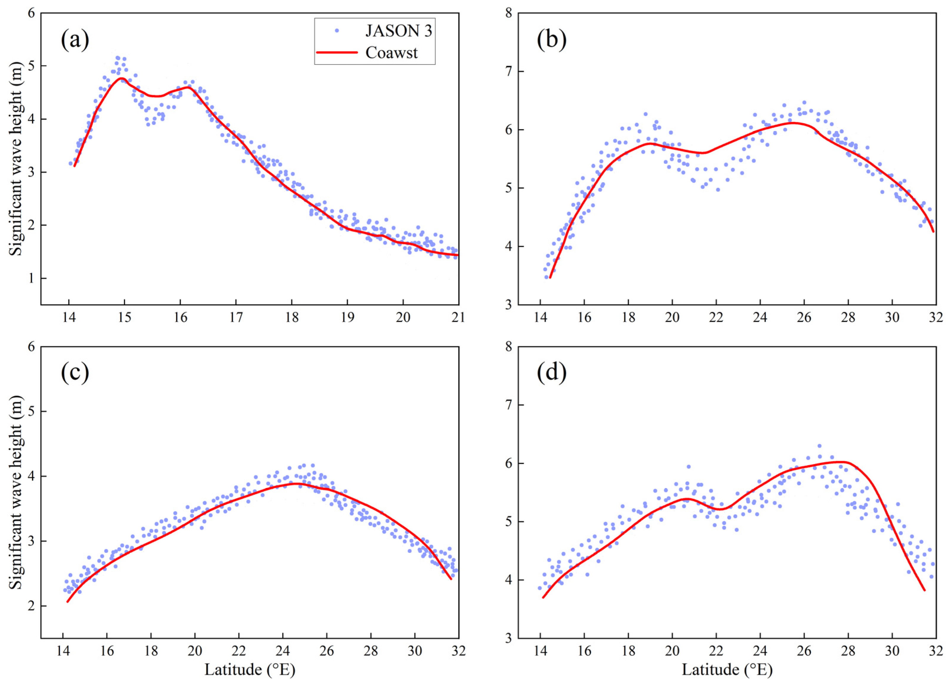
Using HYCOM data as the background field, GFS reanalysis wind fields and ERA5 reanalysis heat flux data as driving fields, the simulated significant wave heights, SST and other variables from the COAWST sea–wave–air coupled model closely match actual measurements. This accuracy suggests that the selection of background fields, initial conditions and physical parameters is appropriate, indicating that the model performs well in simulating sea–wave–air interactions and can serve as a reference for future simulations.

(2)

The inclusion of wave-induced mixing effects in the COAWST model reduces SST biases, particularly in areas affected by the typhoon. The spatial distribution of SST differences aligns with the distribution of significant wave heights, showing larger differences near the typhoon and smaller differences in calmer waters. Analysis reveals that wave-induced vertical mixing enhances current velocities during the typhoon, with a more pronounced effect on the right side of the typhoon path. This enhancement increases upper-layer water dispersion and upwelling, resulting in reduced SST. Furthermore, the MLD metrics in EXP3 demonstrate significant improvements, with the percentage error (PE) decreasing from 26.54 in EXP1 to 18.54, the mean absolute error (MAE) from 8.85 to 5.25 and the root mean square error (RMSE) from 11.05 to 6.13, while the correlation coefficient (COR) increased from 0.84 to 0.92, indicating a notable reduction in errors and enhanced predictive accuracy. For MLT, EXP3 achieves a PE reduction to 1.02, with MAE and RMSE values dropping to 0.41 and 0.46, respectively. Incorporating wave-induced mixing effects thus significantly improves the accuracy of upper-layer SST simulations.

(3)

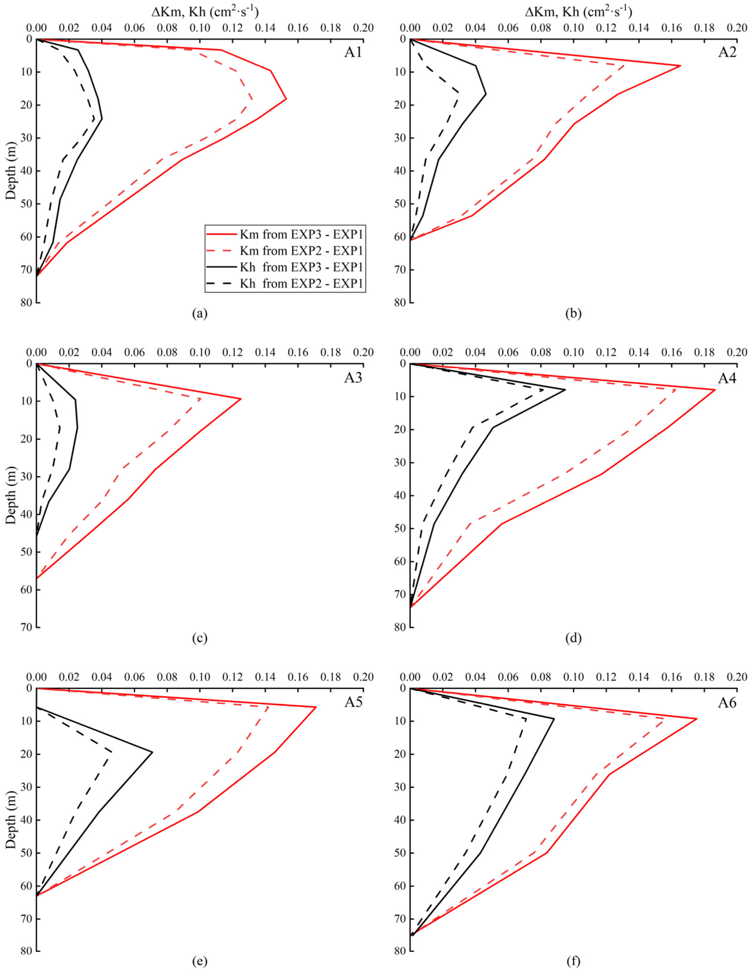
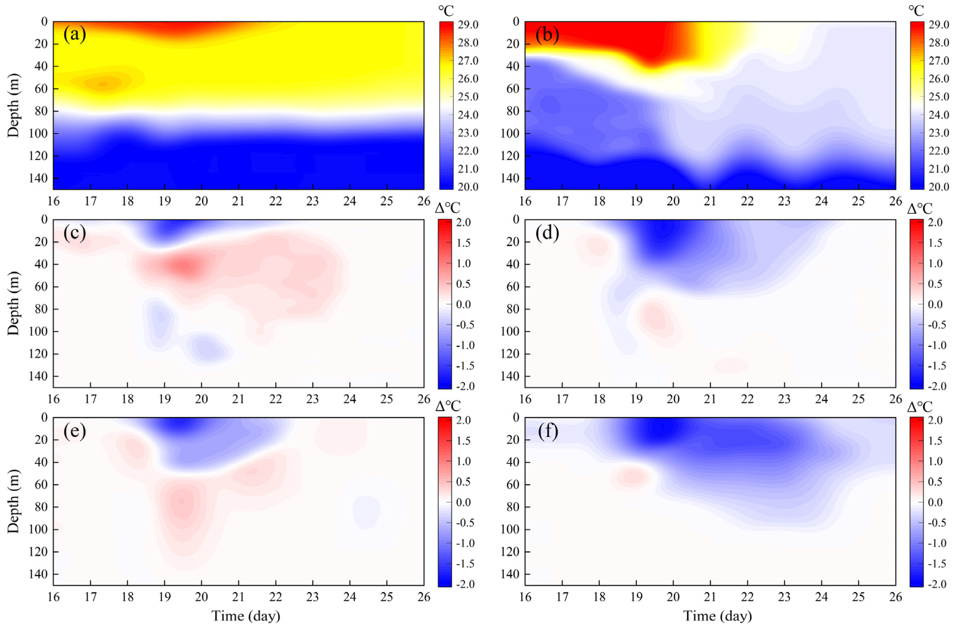
The original COAWST model’s MY2.5 scheme (EXP1) tends to overestimate upper-ocean temperatures, while the previously proposed parameterization scheme (EXP2) underestimates turbulent mixing during typhoons. This paper proposes a new parameterization scheme (EXP3) that accounts for turbulence enhancement during typhoons. Compared to EXP1 and EXP2, EXP3 significantly improves simulations of temperature changes in both the sea surface layer and deep sea column, demonstrating more efficient vertical momentum and heat transfer. Due to strong wind stress and wave breaking caused by intense winds, the upper ocean experiences rapid mixing, leading to a sharp increase in turbulent kinetic energy (TKE), which peaks near the typhoon’s eye. Simulation results indicate that wave-induced mixing significantly enhances the generation and vertical transport of TKE. Specifically, the EXP3 scheme shows that with the inclusion of wave-induced mixing effects, TKE distribution becomes more widespread and intense, leading to an increase in mixed layer depth. This underscores the critical role of wave-induced mixing in enhancing vertical mixing and energy transfer, particularly near the typhoon path. Comparisons of the simulation results from EXP1, EXP2 and EXP3 reveal that the increase in TKE contributes to a more uniform energy distribution within the mixed layer, facilitating vertical heat and momentum exchange. As a result, sea surface temperatures decrease, and the temperature within the mixed layer becomes more uniform. Comparisons with Argo and Drifter buoy data show that EXP3 results are closer to observed measurements, highlighting the importance of incorporating wave-induced mixing and turbulence enhancement. The enhanced model offers better simulations of ocean temperature and current velocity changes during typhoons, improving forecasting accuracy and reliability. This method of improving wave–current interaction modeling is effective and recommended for forecasting sea states in the East China Sea and South China Sea, especially under typhoon conditions. In future research, we will explore the impact of multiple wave effects on the ocean during typhoons using the COAWST model, while also considering the extension of the new wave-induced mixing scheme to global climate models. This extension aims to verify its applicability across different ocean areas and assess its potential impact on the global climate system.

References

1. Zhang, X.; Gao, S.; Ji, X.; Zhu, X.; Zheng, J.; Guo, S. Impact of Typhoons on the Ecological Environment of the Pearl River Estuary in the Summer of 2021—A Study of an Algal Bloom Event. Front. Mar. Sci. 2024, 11, 1395804. [Google Scholar] [CrossRef]
2. Woo, H.J.; Park, K.A. Estimation of Extreme Significant Wave Height in the Northwest Pacific Using Satellite Altimeter Data Focused on Typhoons (1992–2016). Remote Sens. 2021, 13, 1063. [Google Scholar] [CrossRef]
3. Liu, G.; Zhou, X.; Kou, Y.; Wu, F.; Zhao, D.; Yu, Z. Analysis of Extreme Sea States under the Impact of Typhoon in Different Periods: A Nested Stochastic Compound Distribution Applied in the South China Sea. Appl. Ocean Res. 2022, 127, 103298. [Google Scholar] [CrossRef]
4. Wang, Y.; Liu, J.; Du, X.; Liu, Q.; Liu, X. Temporal-Spatial Characteristics of Storm Surges and Rough Seas in Coastal Areas of Mainland China from 2000 to 2019. Nat. Hazards 2021, 107, 1273–1285. [Google Scholar] [CrossRef]
5. Shi, X.; Han, Z.; Fang, J.; Tan, J.; Guo, Z.; Sun, Z. Assessment and Zonation of Storm Surge Hazards in the Coastal Areas of China. Nat. Hazards 2020, 100, 39–48. [Google Scholar]
6. Huang, S.; Du, Y.; Yi, J.; Liang, F.; Qian, J.; Wang, N.; Tu, W. Understanding Human Activities in Response to Typhoon Hato from Multi-Source Geospatial Big Data: A Case Study in Guangdong, China. Remote Sens. 2022, 14, 1269. [Google Scholar] [CrossRef]
7. Wang, T.; Yin, K.; Li, Y.; Chen, L.; Xiao, C.; Zhu, H.; van Westen, C. Physical Vulnerability Curve Construction and Quantitative Risk Assessment of a Typhoon-Triggered Debris Flow via Numerical Simulation: A Case Study of Zhejiang Province, SE China. Landslides 2024, 21, 1333–1352. [Google Scholar] [CrossRef]
8. Li, Y.; Zhao, S.; Wang, G. Spatiotemporal Variations in Meteorological Disasters and Vulnerability in China During 2001–2020. Front. Earth Sci. 2021, 9, 789523. [Google Scholar] [CrossRef]
9. Song, G.; Zhao, L.; Chai, F.; Liu, F.; Li, M.; Xie, H. Summertime Oxygen Depletion and Acidification in Bohai Sea, China. Front. Mar. Sci. 2020, 7, 252. [Google Scholar] [CrossRef]
10. He, T.; Li, J.; Xie, L.; Zheng, Q. Response of Chlorophyll-a to Rainfall Event in the Basin of the South China Sea: Statistical Analysis. Mar. Environ. Res. 2024, 199, 106576. [Google Scholar] [CrossRef]
11. Wang, Y.; Qiao, F.; Fang, G.; Wei, Z. Application of Wave-Induced Vertical Mixing to the K Profile Parameterization Scheme. J. Geophys. Res. Oceans 2010, 115. [Google Scholar] [CrossRef]
12. Mellor, G.L.; Yamada, T. Development of a Turbulence Closure Model for Geophysical Fluid Problems. Rev. Geophys. 1982, 20, 851–875. [Google Scholar] [CrossRef]
13. Price, J.F.; Weller, R.A.; Pinkel, R. Diurnal Cycling: Observations and Models of the Upper Ocean Response to Diurnal Heating, Cooling, and Wind Mixing. J. Geophys. Res. 1986, 91, 8411–8427. [Google Scholar] [CrossRef]
14. Large, W.G.; McWilliams, J.C.; Doney, S.C. Oceanic Vertical Mixing: A Review and a Model with a Nonlocal Boundary Layer Parameterization. Rev. Geophys. 1994, 32, 363–403. [Google Scholar] [CrossRef]
15. Kraus, E.B.; Turner, J.S. A One-Dimensional Model of the Seasonal Thermocline II. Gen. Theory Its Conseq. Tellus 1967, 19, 98–106. [Google Scholar] [CrossRef]
16. Mellor, G.L.; Yamada, T. A Hierarchy of Turbulence Closure Models for Planetary Boundary Layers. J. Atmos. Sci. 1974, 31, 1791–1806. Available online: https://journals.ametsoc.org/view/journals/atsc/31/7/1520-0469_1974_031_1791_ahotcm_2_0_co_2.xml (accessed on 8 July 2024). [CrossRef]
17. Gaspar, P.; Grégoris, Y.; Lefevre, J. A Simple Eddy Kinetic Energy Model for Simulations of the Oceanic Vertical Mixing: Tests at Station Papa and Long-term Upper Ocean Study Site. J. Geophys. Res. 1990, 95, 16179–16193. [Google Scholar] [CrossRef]
18. Craig, P.D.; Banner, M.L. Modeling Wave-Enhanced Turbulence in the Ocean Surface Layer. J. Phys. Oceanogr. 1994, 24, 2546–2559. Available online: https://journals.ametsoc.org/view/journals/phoc/24/12/1520-0485_1994_024_2546_mwetit_2_0_co_2.xml (accessed on 8 July 2024). [CrossRef]
19. The Development of a Coastal Circulation Numerical Model: 1. Wave-Induced Mixing and Wave-Current Interaction. Available online: https://xueshu.baidu.com/usercenter/paper/show?paperid=edacbbfeb14000b0eee6664d208ee0c5 (accessed on 25 July 2024).
20. Uchiyama, Y.; McWilliams, J.C.; Shchepetkin, A.F. Wave–Current Interaction in an Oceanic Circulation Model with a Vortex-Force Formalism: Application to the Surf Zone. Ocean Model. 2010, 34, 16–35. [Google Scholar] [CrossRef]
21. Qiao, F.; Yuan, Y.; Yang, Y.; Zheng, Q.; Xia, C.; Ma, J. Wave-induced Mixing in the Upper Ocean: Distribution and Application to a Global Ocean Circulation Model. Geophys. Res. Lett. 2004, 31. [Google Scholar] [CrossRef]
22. Yang, Y.; Shi, Y.; Yu, C.; Teng, Y.; Sun, M. Study on Surface Wave-Induced Mixing of Transport Flux Residue under Typhoon Conditions. J. Ocean. Limnol. 2019, 37, 1837–1845. [Google Scholar] [CrossRef]
23. Yuan, Y.; Qiao, F.; Yin, X.; Han, L. Analytical Estimation of Mixing Coefficient Induced by Surface Wave-Generated Turbulence Based on the Equilibrium Solution of the Second-Order Turbulence Closure Model. Sci. China Earth Sci. 2013, 56, 71–80. [Google Scholar] [CrossRef]
24. McWilliams, J.C.; Sullivan, P.P. Vertical Mixing by Langmuir Circulations. Spill Sci. Technol. Bull. 2000, 6, 225–237. [Google Scholar] [CrossRef]
25. Smyth, W.D.; Skyllingstad, E.D.; Crawford, G.B.; Wijesekera, H. Nonlocal Fluxes and Stokes Drift Effects in the K-Profile Parameterization. Ocean Dyn. 2002, 52, 104–115. [Google Scholar] [CrossRef]
26. Roekel, L.P.V.; Fox-Kemper, B.; Sullivan, P.P.; Hamlington, P.E.; Haney, S.R. The Form and Orientation of Langmuir Cells for Misaligned Winds and Waves. J. Geophys. Res. Oceans 2012, 117. [Google Scholar] [CrossRef]
27. Noh, Y.; Ok, H.; Lee, E.; Toyoda, T.; Hirose, N. Parameterization of Langmuir Circulation in the Ocean Mixed Layer Model Using LES and Its Application to the OGCM. J. Phys. Oceanogr. 2016, 46, 57–78. [Google Scholar] [CrossRef]
28. Qing, L.; Baylor, F.K. Assessing the Effects of Langmuir Turbulence on the Entrainment Buoyancy Flux in the Ocean Surface Boundary Layer. J. Phys. Oceanogr. 2017, 47, 2863–2886. [Google Scholar]
29. Ali, A.; Christensen, K.H.; Breivik, Ø.; Malila, M.; Raj, R.P.; Bertino, L.; Chassignet, E.P.; Bakhoday-Paskyabi, M. A Comparison of Langmuir Turbulence Parameterizations and Key Wave Effects in a Numerical Model of the North Atlantic and Arctic Oceans. Ocean Model. 2019, 137, 76–97. [Google Scholar] [CrossRef]
30. Wang, H.; Dong, C.; Yang, Y.; Gao, X. Parameterization of Wave-Induced Mixing Using the Large Eddy Simulation (LES) (I). Atmosphere 2020, 11, 207. [Google Scholar] [CrossRef]
31. Han, S.; Wang, M.; Peng, B. Response of Temperature to Successive Typhoons in the South China Sea. J. Mar. Sci. Eng. 2022, 10, 1157. [Google Scholar] [CrossRef]
32. Jacob, S.D.; Shay, L.K.; Mariano, A.J.; Black, P.G. The 3D Oceanic Mixed Layer Response to Hurricane Gilbert. J. Phys. Oceanogr. 2000, 30, 1407–1429. [Google Scholar] [CrossRef]
33. Huang, P.; Sanford, T.B.; Imberger, J. Heat and Turbulent Kinetic Energy Budgets for Surface Layer Cooling Induced by the Passage of Hurricane Frances (2004). J. Geophys. Res. Oceans 2009, 114. [Google Scholar] [CrossRef]
34. Kantha, L.H.; Clayson, C.A. An Improved Mixed Layer Model for Geophysical Applications. J. Geophys. Res. 1994, 99, 25235–25266. [Google Scholar] [CrossRef]
35. Martin, P.J. Simulation of the Mixed Layer at OWS November and Papa with Several Models. J. Geophys. Res. 1985, 90, 903–916. [Google Scholar] [CrossRef]
36. Wang, J.; Kuang, C.; Chen, K.; Fan, D.; Qin, R.; Han, X. Wave–Current Interaction by Typhoon Fongwong on Saline Water Intrusion and Vertical Stratification in the Yangtze River Estuary. Estuar. Coast. Shelf Sci. 2022, 279, 108138. [Google Scholar] [CrossRef]
37. Zhang, W.; Li, R.; Zhu, D.; Zhao, D.; Guan, C. An Investigation of Impacts of Surface Waves-Induced Mixing on the Upper Ocean under Typhoon Megi (2010). Remote Sens. 2023, 15, 1862. [Google Scholar] [CrossRef]
38. Qiao, F.; Yuan, Y.; Ezer, T.; Xia, C.; Yang, Y.; Lü, X.; Song, Z. A Three-Dimensional Surface Wave–Ocean Circulation Coupled Model and Its Initial Testing. Ocean Dyn. 2010, 60, 1339–1355. [Google Scholar] [CrossRef]
39. Sun, Z.; Shao, W.; Yu, W.; Li, J. A Study of Wave-Induced Effects on Sea Surface Temperature Simulations during Typhoon Events. J. Mar. Sci. Eng. 2021, 9, 622. [Google Scholar] [CrossRef]
40. Yao, R.; Shao, W.; Hao, M.; Zuo, J.; Hu, S. The Respondence of Wave on Sea Surface Temperature in the Context of Global Change. Remote Sens. 2023, 15, 1948. [Google Scholar] [CrossRef]
41. Huang, C.J.; Qiao, F. Wave-Turbulence Interaction and Its Induced Mixing in the Upper Ocean. J. Geophys. Res. Oceans 2010, 115. [Google Scholar] [CrossRef]
42. Ma, H.; Dai, D.; Guo, J.; Qiao, F. Observational Evidence of Surface Wave-Generated Strong Ocean Turbulence. J. Geophys. Res. Oceans 2020, 12, e2019JC015657. [Google Scholar] [CrossRef]
43. Study on Hydrodynamic Environment of the Bohai Sea, the Huanghai Sea and the East China Sea with Wave-Current Coupled Numerical Model. Available online: http://www.hyxbocean.cn/en/article/id/20040403 (accessed on 25 July 2024).
44. Pleskachevsky, A.; Dobrynin, M.; Babanin, A.V.; Günther, H.; Stanev, E. Turbulent Mixing Due to Surface Waves Indicated by Remote Sensing of Suspended Particulate Matter and Its Implementation into Coupled Modeling of Waves, Turbulence, and Circulation. J. Phys. Oceanogr. 2011, 41, 708–724. [Google Scholar] [CrossRef]
45. Skamarock, W.C.; Klemp, J.B.; Dudhia, J.; Gill, D.O.; Barker, D.M.; Duda, M.G.; Huang, X.-Y.; Wang, W.; Powers, J.G. A Description of the Advanced Research WRF Version 3; National Center for Atmospheric Research: Boulder, CO, USA, 2008; Volume 1, pp. 1–5. [Google Scholar] [CrossRef]
46. Booij, N.; Ris, R.C.; Holthuijsen, L.H. A Third-generation Wave Model for Coastal Regions: 1. Model Description and Validation. J. Geophys. Res. 1999, 104, 7649–7666. [Google Scholar] [CrossRef]
47. Shchepetkin, A.F.; McWilliams, J.C. The Regional Oceanic Modeling System (ROMS): A Split-Explicit, Free-Surface, Topography-Following-Coordinate Oceanic Model. Ocean Model. 2004, 9, 347–404. [Google Scholar] [CrossRef]
48. Warner, J.C.; Armstrong, B.; He, R.; Zambon, J.B. Development of a Coupled Ocean–Atmosphere–Wave–Sediment Transport (COAWST) Modeling System. Ocean Model. 2010, 35, 230–244. [Google Scholar] [CrossRef]
49. Lin, S.; Zhang, W.Z.; Wang, Y.; Chai, F. Mechanism of Oceanic Eddies in Modulating the Sea Surface Temperature Response to a Strong Typhoon in the Western North Pacific. Front. Mar. Sci. 2023, 10, 1117301. [Google Scholar] [CrossRef]
50. Yang, B.; Hou, Y.; Hu, P.; Liu, Z.; Liu, Y. Shallow Ocean Response to Tropical Cyclones Observed on the Continental Shelf of the Northwestern S Outh C Hina S Ea. J. Geophys. Res. Oceans 2015, 120, 3817–3836. [Google Scholar] [CrossRef]
51. Chen, H.; Li, S.; He, H.; Song, J.; Ling, Z.; Cao, A.; Zou, Z.; Qiao, W. Observational Study of Super Typhoon Meranti (2016) Using Satellite, Surface Drifter, Argo Float and Reanalysis Data. Acta Oceanol. Sin. 2021, 40, 70–84. [Google Scholar] [CrossRef]
52. Song, Z.; Qiao, F.; Song, Y. Response of the Equatorial Basin-Wide SST to Non-Breaking Surface Wave-Induced Mixing in a Climate Model: An Amendment to Tropical Bias. J. Geophys. Res. Oceans 2012, 117. [Google Scholar] [CrossRef]
53. Sun, J.; Oey, L.-Y.; Chang, R.; Xu, F.; Huang, S.-M. Ocean Response to Typhoon Nuri (2008) in Western Pacific and South China Sea. Ocean Dyn. 2015, 65, 735–749. [Google Scholar] [CrossRef]
54. Zhang, H.; Liu, X.; Wu, R.; Chen, D.; Zhang, D.; Shang, X.; Wang, Y.; Song, X.; Jin, W.; Yu, L.; et al. Sea Surface Current Response Patterns to Tropical Cyclones. J. Mar. Syst. 2020, 208, 103345. [Google Scholar] [CrossRef]
55. Hazelworth, J.B. Water Temperature Variations Resulting from Hurricanes. J. Geophys. Res. 1968, 73, 5105–5123. [Google Scholar] [CrossRef]
56. Li, M.; Garrett, C.; Skyllingstad, E. A Regime Diagram for Classifying Turbulent Large Eddies in the Upper Ocean. Deep-Sea Res. Part I 2004, 52, 259–278. [Google Scholar] [CrossRef]
57. Wadler, J.B.; Cione, J.J.; Michlowitz, S.; de la Cruz, B.J.; Shay, L.K. Improving the Statistical Representation of Tropical Cyclone In-Storm Sea Surface Temperature Cooling. Weather Forecast. 2024, 39, 847–866. [Google Scholar] [CrossRef]
58. Roemmich, D.; Owens, W. The Argo Project: Global Ocean Observations for Understanding and Prediction of Climate Variability. Oceanography 2000, 13, 45–50. [Google Scholar] [CrossRef]
59. Hasselmann, K. Wave-Driven Inertial Oscillations. Geophys. Fluid Dyn. 1970, 1, 463–502. [Google Scholar] [CrossRef]
60. Clement, U.; Gérald, D.; Lucile, G.; Aurélien, P.; Fabrice, A.; Maxime, B.; Yannice, F. Reconstructing Ocean Surface Current Combining Altimetry and Future Spaceborne Doppler Data. J. Geophys. Res. Oceans 2021, 126. [Google Scholar] [CrossRef]
Figure 1. Schematic diagram of COAWST: (a) Data exchange rationale for the COAWST model; (b) layout of the experimental setup for the COAWST model in this paper.
Remotesensing 16 03298 g001
Figure 2. Schematic diagram of the COAWST computational domain and nested grids.
Remotesensing 16 03298 g002
Figure 3. Map of the study area: (a) typhoon track and intensity; (b) location of selected Argo buoys and analysis points; (c) Jason-3 satellite altimeter track; (d) yrack of selected Drifter buoy.
Remotesensing 16 03298 g003
Figure 4. Spatial distribution of SWH during the typhoon transit (af) (black arrows indicate the wave direction, and colors indicate the SWH intensity).
Remotesensing 16 03298 g004
Figure 5. Evaluation of simulated SWH data against observations from the Jason-3 satellite (ad).
Remotesensing 16 03298 g005
Figure 6. Spatial distribution of sea surface velocities during typhoon transit (af).
Remotesensing 16 03298 g006
Figure 7. Difference between simulated SST values and OISST values during typhoon transit. The left column (a,d,g) represents the results of the EXP1 scheme, the middle column (b,e,h) represents the results of the EXP2 scheme and the right column (c,f,i) represents the results of the EXP3 scheme. Each row corresponds to a different time period.
Remotesensing 16 03298 g007
Figure 8. Spatial distribution of sea surface temperature differences due to wave mixing during typhoon transit (af): (a,c,e) the simulation results of EXP3-EXP1; (b,d,f) the simulation results of EXP2-EXP1.
Remotesensing 16 03298 g008
Figure 9. Comparison of simulated and buoy-measured temperature profiles A1–A6), and the dashed line is the depth of the mixed layer under this experiment (following the buoy position in Figure 3d).
Remotesensing 16 03298 g009
Figure 10. Km and Kh at selected buoy locations (af).
Remotesensing 16 03298 g010
Figure 11. MLD, MLT time series plots of Argo observations versus two experiments (a,b). Scatter plots of buoy observations of MLD and MLT versus model results and the associated linear best-fit lines (c,d). Observations were taken from buoys that were within the typhoon’s influence during the typhoon (locations of buoys are shown in Figure 3d).
Remotesensing 16 03298 g011
Figure 12. Time series plots of temperature variations at different sites and experimental protocols: (a) EXP1 at site B1; (b) EXP1 at site B2; (c) EXP2-EXP1 at site B1; (d) EXP2-EXP1 at site B2; (e) EXP3-EXP1 at site B1; and (f) EXP3-EXP1 at site B2.
Remotesensing 16 03298 g012
Figure 13. Comparison of simulated and buoy-measured sea surface current velocities (ad) (Corresponding to buoys D1 through D4 shown in Figure 3d).
Remotesensing 16 03298 g013
Figure 14. Surface flow vector fields (ac) before, during, and after the typhoon (green asterisks indicate the location of the typhoon, black arrows indicate results for EXP1, blue arrows indicate results for EXP2 and red arrows indicate results for EXP3).
Remotesensing 16 03298 g014